1. Introduction
The traditional ‘Dutch book’ and ‘representation theorem’ arguments for probabilism (the thesis that a rational agent’s degrees of belief ought to satisfy the probability axioms) rely on a connection between credences and practical rationality that some have found problematic.Footnote 1 Starting at least with Joyce (Reference Joyce1998), many formal epistemologists have sought to replace these arguments with more purely epistemic ones that focus on a notion of ‘accuracy’. This is understood as a purely epistemic good, representing something like the ‘distance’ between one’s credences and the actual truth values of the propositions one considers. In this article, I will extend some recent arguments of this sort, to show that accuracy considerations can give stronger requirements than have been thought. This can be seen as either a strength or a weakness for the accuracy-based approach.
Hannes Leitgeb and Richard Pettigrew (Reference Leitgeb and Pettigrew2010a, Reference Leitgeb and Pettigrew2010b) use accuracy conditions to support not only probabilism but also the diachronic norm of conditionalization (that one’s credence in A after learning B is given by  , when that is defined), which is characteristic of Bayesianism. They show that their arguments work if the set of worlds that are taken to be possibilities by the agent is finite, and ask at the end of each paper how their arguments fare if the set of worlds is allowed to be infinite.
I will show that the argument does extend to infinite sets of worlds, if we make a few natural assumptions about how to understand various concepts that they only explicitly discuss for finite cases. Consideration of the methodology in infinite settings gives arguments for even more norms beyond the ones that Leitgeb and Pettigrew endorse. In particular, it seems to give arguments for principles like those known as ‘conglomerability’ and ‘reflection’. (See sec. 3.2 for precise statements of these principles.) This may be seen as a further strength of the methodology, or (because of existing arguments against these principles) a reductio of the methodology, or a call to further investigate the methodology to find reasons to accept the arguments of Leitgeb and Pettigrew without accepting these further conclusions. It is not my goal in this article to decide between these three responses, but merely to propose them as questions for future research.
My arguments will be similar to Leitgeb and Pettigrew’s argument for conditionalization (sec. 6.2 of their second paper) rather than to their argument for probabilism (sec. 6.1) or their more tentative arguments for uniform distribution (sec. 6.3) and a highly nonstandard alternative to Jeffrey conditionalization (sec. 7). This argument is very similar to the one given by Hilary Greaves and David Wallace (Reference Greaves and Wallace2006, 608) that, “under independently motivated conditions, conditionalization maximizes expected epistemic utility.” As I set up my framework, I will show how my argument relates to each of these.
Leitgeb and Pettigrew (Reference Leitgeb and Pettigrew2010a, 209) say “there is nothing particularly philosophical about our decision to stick to the case of finitely many worlds in this article; we simply assume this to be so and postpone the discussion of the infinite case to another time.” Similarly, Greaves and Wallace (Reference Greaves and Wallace2006, 611 n. 1) state, “We will assume throughout that  [the set of states] is finite. This is merely for simplicity of exposition.” (They similarly assume that no nonempty proposition has credence 0.) As it turns out, even describing the argument requires some more substantive assumptions if
 can be infinite rather than if it is finite. However, the appropriately modified arguments do work, giving an argument not just for conditionalization but for (versions of) conglomerability and reflection.
In section 2, I will outline the features used in the infinite version of the argument. The first four parts discuss the general framework, and the fifth discusses special issues surrounding the notion of expected value in an infinite setting. The section concludes with precise statements of my three main theorems: roughly, that a conditional probability function that minimizes expected inaccuracy satisfies the ratio formula (when that is defined) and takes on a range of values whose expectation is the unconditional probability, which must therefore lie within the range spanned by the conditional probabilities. (Proofs are given in the appendix.)
In section 3, I discuss the interpretation of these theorems. In particular, I consider their import for both synchronic coherence of an agent’s attitudes and what I consider more speculative diachronic norms like those suggested by Leitgeb and Pettigrew, and Greaves and Wallace. I end with a brief conclusion and an appendix containing proofs of the theorems.
2. Assumptions of the Setting
2.1. Propositions, Probability, and Measurability
For the purposes of this discussion, I treat the objects of doxastic attitudes as propositions and think of propositions as sets of possibilities.Footnote 2 Each proposition is identified with a subset of the set  of possibilities for the agent.
I will also assume that the synchronic norms of probabilism have already been established, perhaps by means of the argument that Leitgeb and Pettigrew use, or perhaps independently. Thus, I will assume that the agent’s credences satisfy the axioms of probability theory, and, to emphasize this fact, I will use ‘P’ as the name for the function that represents the credences. To be explicit, this means:
1. Whenever
 is defined, .
2.
.3. If A and B are disjoint subsets of
, then, whenever and are both defined, is defined and equal to .
 is defined,
 .
 .
 , then, whenever
 and
 are both defined,
 is defined and equal to
 .
The condition that these credences are defined turns out to be important for the generalization to the infinite case. It is well-known that in many infinite sets, some natural constraints on probabilities are incompatible with every subset having a probability. Instead, we must assign probabilities only to some collection  of the ‘measurable’ subsets of the space. In standard measure theory, it is assumed that
 is a σ-field. This means:
1.
is a member of .2. If A is in
, then (the complement of A in ) is in .3. If
are countably many members of , then their union is in .
 is a member of
 .
 , then
 (the complement of A in
 ) is in
 .
 are countably many members of
 , then their union
 is in
 .
By suitable applications of these assumptions, one can show that countable intersections of members of  are in
 too.
Thus, I will not assume that the agent has credences in every proposition, but I will let  be the set of propositions for which she does have credences, and I will assume that
 is a σ-field. Of course, if the agent does have credences in every proposition, then
 is trivially a σ-field. I suspect that the closure properties of
 can be weakened somewhat, though this may complicate some of the arguments.
2.2. Updates and Experiments
Not all updates fall in the scope of my argument. I will only consider updates on which  remains fixed. Situations in which the agent comes to have credences in new propositions seem very different from the standard examples where an agent just learns that some proposition is true. For instance, two natural cases where
 would be expected to change are the introduction of a new theory, and the discovery of confusion in one’s old concepts, either one of which might be part of something like a scientific revolution. Bayesians already know (Earman Reference Earman1992) that these cases are difficult ones to account for.
I will follow Greaves and Wallace in considering an update situation as being given in advance by some experiment: “[An experiment is] a situation in which the agent is to receive some new piece of information, from among a set of mutually exclusive and jointly exhaustive alternatives. Mathematically, an experiment is represented by a partition  of
 ” (Greaves and Wallace Reference Greaves and Wallace2006, 611). To say that
 is a partition of
 just means that
 is a collection of propositions such that each member of
 is in exactly one of the propositions in
 . Since their
 is finite, so is any experiment
 for them. But I will allow
 to be infinite.
As a simple example, we can imagine that the agent is about to flip a coin and observe how it lands. We can think of  as the set
 , where H is the set of all possibilities in which the coin lands “heads,” and T is the set of all possibilities in which the coin lands “tails.” For a more complicated example, consider the experiment of consulting an oracle to ask how many humans will ever have lived. In this case, it seems reasonable that any sufficiently large integer is an epistemically possible outcome, though we might imagine that there are other possible outcomes as well, such as one in which the oracle says, “I don’t know.” The experiment is represented by the set of distinguishable outcomes for the agent—in this case, rather than one member of
 being the set of worlds in which there are exactly 10 trillion humans over the history of the universe, the relevant member of
 is the set of worlds in which the oracle says “10 trillion” in answer to the question. Yet more complicated examples may arise in cases where the agent is about to throw an infinitely thin dart at a dart board—if the agent can distinguish each infinitely small point of the board, then the elements of
 will correspond to each possible landing site of the dart, but if the agent cannot distinguish these points perfectly, then the elements of
 will be much more complicated.
As suggested by my examples, the sort of experiment I consider is one in which the agent comes to have credence 1 in exactly one member of  and credence 0 in all the rest. Cases in which the update is generated in some other way (e.g., cases driven by conditional probability [van Fraassen Reference van Fraassen1981], cases involving potential memory loss [Arntzenius Reference Arntzenius2003], and cases calling for Jeffrey conditionalization—or the alternative to it that Leitgeb and Pettigrew [Reference Leitgeb and Pettigrew2010b, 252–60.] propose) are beyond the scope of the arguments considered here. However, the notion of conditional probability is traditionally thought to play an important role in these updates, and if the concept of conditional probability can be clarified by my arguments, then they will at least indirectly help us understand these more complicated updates.
I will also assume that  is a subset of
 —each distinguishable outcome of the experiment had some credence for the agent prior to the experiment being performed. In cases where some elements of
 are not in
 , the agent has a possibility of coming to know some proposition that she does not already grasp—thus, they are outside the scope of my arguments. Updates involving indexicals like ‘here’ or ‘today’ have this feature, so my arguments do not directly apply to “Sleeping Beauty” or related cases (Meacham Reference Meacham2008; Titelbaum Reference Titelbaum2008; Bradley Reference Bradley2012).
2.3. Plans and Availability
I will consider an update as proceeding according to a set of “plans” for an experiment.Footnote 3 For a given experiment  , and for each proposition A in
 , I will represent the agent’s plan for updating her credence in A after performing
 as a function
 that gives a real number in each state. For any state s in
 ,
 is the credence that the agent plans to have in A after learning the outcome of
 , if s is the actual state. When
 is understood from context, I will sometimes refer to just
 .
This use of “plans” distinguishes my framework slightly from those of Leitgeb and Pettigrew, and Greaves and Wallace. Leitgeb and Pettigrew think of an update as given by a single proposition E that the agent becomes certain of. In the case where  is finite and all its members have positive prior credence, it will turn out that the difference is inessential. However, when some members of
 have prior credence 0 (and in many cases, such as ones where the experiment consists of learning the precise real value of some unknown physical parameter, it may be the case that all members of
 have prior credence 0), the partition will play an essential role in the argument. And once we have a partition rather than a single proposition, something like this notion of “plan” is essential.
Greaves and Wallace talk of “acts” whereas I talk of “plans.” The main difference is that while their acts specify a complete probability distribution for the agent in each state, my plans only specify the agent’s credence for a single proposition. This primarily helps simplify some of the discussion, but it is also connected to the distinction between global and local inaccuracy measures, to be discussed in section 2.4.Footnote 4
Of course, given the notion of updates and experiments I am working with, not just any such function will correspond to a possible plan. Only a subset of these functions will be said to be “available.” Since the experiment represents the information the agent comes to know during the course of the update, an agent’s plans must make the same response in states where the outcome of the experiment is the same.
A plan  is said to be available (or “
 -available,” if I need to make explicit which partition is relevant) if and only if it meets the following two conditions:
1. If
and , then .2. If x is any rational number, then
, where is the set of states s for which .
 and
 , then
 .
 , where
 is the set of states s for which
 .
A plan that did not satisfy the first constraint would require the agent’s credence function to depend on information that she does not have, even once the experiment is performed. The terms  and
 are both compatible with all the information that she has so far (which is what it means to be in
 ), and since what she learns on completing
 is just which member of
 is actual, she does not learn anything to distinguish them. Thus, she cannot plan to act differently in those two states.
The second constraint is a bit more subtle. If  is a finite or countable partition, then it is not a further requirement but in fact follows from the first one, together with the fact that
 is a σ-algebra. So it is only a further assumption if
 is uncountably infinite. In planning whether to have credence greater than x, the agent is responding to whether the actual world is in
 or not, and it seems that this responsiveness should require that
 be a proposition she can grasp. (Readers who are familiar with the language of measure theory will recognize this second constraint as the requirement that
 be measurable with respect to the agent’s credence function, which is essential for the notion of expected value to make sense.)
2.4. Inaccuracy, Global and Local
The arguments under consideration are all based on a function I that measures ‘inaccuracy’ of a belief state. The one I will use is what Leitgeb and Pettigrew call a ‘local inaccuracy measure’, which is a function such that  is a real number that measures how epistemically bad it is to have credence x in proposition A in state s. Greaves and Wallace instead describe their function as an ‘epistemic utility function’, but in the terminology of Leitgeb and Pettigrew, it behaves like a ‘global inaccuracy measure’. This is a function U such that
 is a real number that measures how good or bad the overall credence function p is in state s.
Leitgeb and Pettigrew argue that agents should have both local and global inaccuracy measures and that these should cohere in a particular way. As a result, they claim that the local inaccuracy function should be given by the Brier score, which is defined by  if A is true in s and
 if A is false in s. They also argue that the global inaccuracy function should be given by the sum of the local inaccuracies over all propositions. Their arguments are interesting, but they rely on some controversial assumptions about the “geometry of reason” (Leitgeb and Pettigrew Reference Leitgeb and Pettigrew2010a, 210; see also their theorems 3, 4, and 5 on 222–29). In addition, these arguments cannot work when there are infinitely many propositions to be considered—their version of global inaccuracy will normally be infinite and thus cannot relate to local inaccuracy in any interesting way.Footnote 5
Greaves and Wallace make no claims about local inaccuracy measures and very few claims about the global inaccuracy measure that they use. This gives them some greater generality but also requires that they consider an update in terms of “acts” that specify posterior credences for all propositions, rather than my “plans” that specify posterior credence for only a single proposition at a time.
I will instead work just with local inaccuracy measures. I will make five assumptions about the local inaccuracy function  . (These assumptions are weaker than the ones that Leitgeb and Pettigrew make and have parallels in other discussions of inaccuracy, such as Joyce Reference Joyce1998.)
Extensionality. First, I assume that the inaccuracy of having credence x in proposition A does not depend on any feature of the state s other than whether A is true or false. Thus, the function can be thought of as two functions,  and
 , the former assigning inaccuracies in states where A is true and the latter in states where A is false. In cases where A is clear from context, I will suppress the first argument for the function and just talk about
 and
 . (One might further assume that the function is in fact identical for each proposition A, but this is not needed for my arguments.)
Monotonicity. Second, I also assume that for each A,  has its only local or global minimum when
 , while
 has its only local or global minimum when
 . That is,
 is monotonically increasing and
 is monotonically decreasing on
 . If we consider the possibility of credences outside of
 , then both functions should increase as x moves away from this interval.
Bounded Continuity. Third, I assume that for any positive ε and each A there is a set of finitely many values  such that, for every
 ,

and

(Given Monotonicity, this is equivalent to the functions being bounded and continuous on  .)
Convexity. Fourth, for any  and any
 , I assume that
 , and similarly
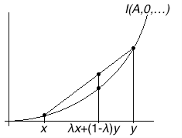
 . As illustrated in figure 1, this means that the inaccuracy of any credence intermediate between x and y is always less than predicted by linear interpolation between the inaccuracies of x and of y. Thus, not only is inaccuracy increasing as one’s estimate gets farther from the truth value, but the rate of increase always increases as well.
Figure 1.

Immodesty. Finally, I assume that if  then the unique value of x that minimizes
 is
 . Once I introduce the notion of ‘expected inaccuracy’ (in sec. 2.5), we will see that, for someone who has
 , this is their estimate of the inaccuracy of someone who has credence x in A. If
 were not the unique minimum, then an agent with credence c would be ‘modest’, in the sense that she would think that some other credence was at least as accurate as her own. This condition is extensively discussed in the literature, sometimes under the name ‘propriety’ (Greaves and Wallace Reference Greaves and Wallace2006; Joyce Reference Joyce, Huber and Schmidt-Petri2009; Myrvold Reference Myrvold2012).
These five assumptions are all satisfied by the Brier score, so they follow from the assumptions made by Leitgeb and Pettigrew. They also follow from Joyce’s assumptions on accuracy and are satisfied by the other scoring rules discussed on page 275 of Joyce (Reference Joyce, Huber and Schmidt-Petri2009). Greaves and Wallace assume only the equivalent of Immodesty for their global inaccuracy measure. But since this is the most arbitrary-seeming assumption, my argument is no worse off than theirs.
2.5. Expected Inaccuracy
Before giving the proofs, I need to explain a bit more about ‘expected inaccuracy’ and show why this notion makes sense. If V is a random variable (i.e., a function that takes on a real value in each state s in  ), then the ‘expected value of V’, notated as
 , represents something like the agent’s best estimate of V. It depends on the values for V in each possible state and the agent’s credence function P. Although
 may be distinct from every possible value of V (just as the average family may have 2.3 children even though no particular family has exactly that many), it traditionally plays a role in guiding one’s actions in light of one’s uncertainty about V.
We can stipulate a definition of the expected value of V with respect to P, as Leitgeb and Pettigrew do. However, they consider at least two different stipulations ( , or
 ), which give distinct results for some infinite cases, and both seem clearly wrong for others.Footnote 6 And there are further worries that arise in taking a sum of infinitely many terms, especially if the series is uncountable.
Thus, instead of stipulatively defining expectation as Leitgeb and Pettigrew do, I will adopt the axiomatic approach of Whittle (Reference Whittle2000). For random variables  , Whittle’s axioms state:
1. If
for all s, then .2. If c is a constant, then
.3.
.4. For an event A, let
be the random variable with if A is true in s and if A is false in s. Then .Footnote 75. If for every s the sequence
is monotonically increasing and converges to , then the sequence is monotonically increasing and converges to .
 for all s, then
 .
 .
 .
 be the random variable with
 if A is true in s and
 if A is false in s. Then
 .
 is monotonically increasing and converges to
 , then the sequence
 is monotonically increasing and converges to
 .
Axiom 1 seems essential to the concept of an expected value. A random variable cannot have a negative expected value unless it is at least possible for it to take on a negative value. Axiom 4 gives the only direct connection between probability and expected value. Axioms 2, 3, and 5 provide linearity conditions on expected value. Axiom 3 is often a surprise to students when they learn that it holds regardless of whether  and
 are independent or dependent. However, once one has convinced oneself that it holds, it is plausible that it is in fact essential to the notion of expected value and not merely a mathematical consequence of a formal definition.
If V is a measurable random variable that always takes either the value v or the value 0, then axioms 2 and 4 guarantee that  . If V is a measurable random variable that takes on only finitely many possible values, then it is the sum of finitely many random variables of the previous sort, and thus, applying axiom 3, we see that
 .
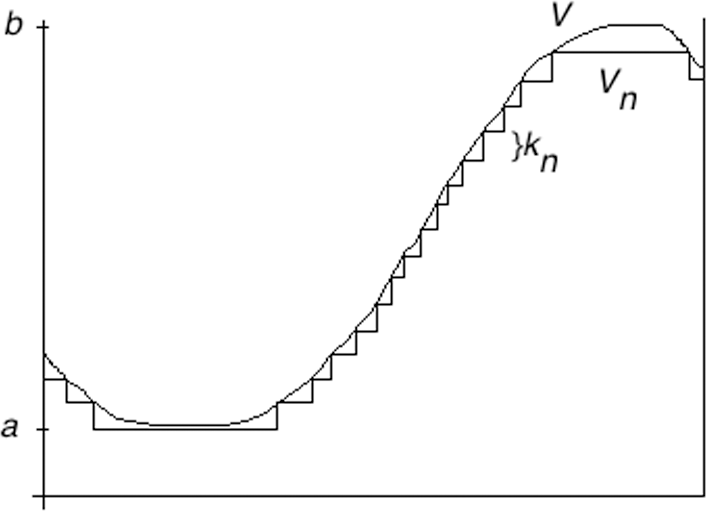
If V is a measurable random variable, and it is bounded (there are a and b with  for all s), then this previous result together with axiom 5 will be sufficient to uniquely determine
 . This is because we can define a sequence of random variables
 that are monotonically increasing and converge to V, each one of which is measurable and takes on only finitely many possible values. In particular, we define
 , and we define
 whenever
 . (See fig. 2.)
Figure 2.

The result of the previous paragraph suffices to define each  , and axiom 5 guarantees that
 is the limit of these values. (This is in fact equivalent to the standard measure-theoretic definition of the expected value of a bounded measurable random variable as a Lebesgue integral.)
If we let  be some available plan for updating one’s credence in A for some experiment
 , and if
 is the inaccuracy
 , then we can see that V is measurable (because
 is measurable, so
 is measurable, and I satisfies Extensionality and Monotonicity, so it is measurable as well) and bounded (because I satisfies Bounded Continuity). Thus, Whittle’s axioms for expectation suffice to define the expected inaccuracy of any plan of the sort I consider.
Without Extensionality, inaccuracy might depend on some proposition for which the agent does not have a credence, so it would not have an expectation. Without Monotonicity and Bounded Continuity, inaccuracy could be unbounded in a way that results in its expected value being infinite or undefined. Thus, some version of these first three assumptions is surely needed for expected inaccuracy to be the sort of thing one could try to minimize.
The use of expected inaccuracy distinguishes the arguments of Leitgeb and Pettigrew, and that of Greaves and Wallace, from some other accuracy-based arguments. For instance, Lindley (Reference Lindley1982) and Joyce (Reference Joyce1998) both give arguments for probabilism (Lindley argues for the ratio analysis of conditional probability as well) based merely on the requirement that no other credence function dominate the one under consideration (one credence function “dominates” another if and only if the first has lower inaccuracy in every state). Since one credence function can have lower expected inaccuracy than another without being dominated, the Joyce and Lindley results are correspondingly stronger. All of these arguments, other than that of Greaves and Wallace, assume a strong connection between global and local accuracy.
My argument (like that of Leitgeb and Pettigrew) makes the stronger assumptions of each, that utility should be defined by a local inaccuracy measure and that agents should rule out all plans with higher expected inaccuracy rather than merely plans that are dominated. If there is some problem in principle with local inaccuracy measures or expected inaccuracy, then this would give a reason to reject my conclusions while accepting the conclusions of some of the others. However, my arguments apply even when  is infinite, and I give results leading to versions of conglomerability and reflection, in addition to the ratio formula for conditional probability. (As an anonymous referee has pointed out, the authors that give dominance arguments rather than expectation arguments are trying to establish probabilism as well as conditionalization. If probabilism is not already taken for granted, then the use of expectation is clearly problematic. But once probabilism is granted, as I have assumed here, the use of expectation rather than dominance may not be a real weakness.)
2.6. The Theorems
The following results are proved in the appendix.
Ratio Theorem. If A is a measurable proposition,  is an experiment, E is an element of
 with positive probability, and
 has minimal expected inaccuracy among the
 -available plans for updating one’s credence in A, then
 for any s in E.
This theorem is the same as theorem 3 in Leitgeb and Pettigrew (Reference Leitgeb and Pettigrew2010b, 250), except for my weaker assumptions on I and the measurability assumptions needed for the infinite case. This is also the same as corollary 1 that Greaves and Wallace state on page 625, except that they only assume Immodesty, while I use a local inaccuracy measure and the measurability assumptions for infinite sets.
Interval Theorem. If A is a measurable proposition,  is an experiment, and
 has minimal expected inaccuracy among the
 -available plans for updating one’s credence in A, then there is no x with
 and
 for all s, and there is no x with
 and
 for all s. That is,
 .
This theorem basically says that no optimal update plan guarantees an increase in credence, or guarantees a decrease in credence. For every experiment that could increase one’s credence in A by some positive ε, there is always some other possible outcome of the experiment that would fail to do so.
In many cases, the content of this theorem can be better understood by looking at a more specific consequence:
Expectation Theorem. If, for all propositions A in  , the conditions of the Interval Theorem hold, and for each s,
 is a probability function (so that
 for all A,
 , and
 whenever A and B are disjoint), then for all A,
 .
That is, the expected result of an update plan for A should equal one’s prior credence in A.
All of these theorems tell us what plans that minimize expected inaccuracy must be like, if they exist. Fortunately, such plans do exist. (The space of possible plans is the set of functions from  to
 , which is compact, by Tychonov’s theorem. Expected inaccuracy is a continuous function on the space of plans and must therefore achieve its minimum value.)
The extra condition in the statement of the Expectation Theorem is a bit subtle. In particular, since I have a separate plan for each proposition, I have not assumed that the plans will combine to yield a coherent posterior probability function. And in fact, if  is a countable partition of propositions whose credences fail to sum to 1, then it is known that the conclusion of the Expectation Theorem must be violated, so there can be no set of plans that cohere probabilistically (Hill and Lane Reference Hill and Lane1985, 369). However, if the unconditional credences satisfy countable additivity (as orthodox Bayesianism assumes), then the Radon-Nikodym theorem of real analysis guarantees the existence of coherent update plans that satisfy the conclusions of all three theorems. It remains to be seen if such plans must always minimize expected inaccuracy, but it seems plausible that they will.
When  is finite, the Interval Theorem and Expectation Theorem are trivial consequences of the Ratio Theorem. It is only in the infinite case that these provide additional content. Thus, the normative claims about updating and conditional credence that I discuss in the next section all apply to the finite case as a consequence of the arguments by Leitgeb and Pettigrew or Greaves and Wallace. My contribution is to show that they hold in the infinite case as well.
3. Normative Applications of the Theorems
3.1. Accuracy Only?
In much of the literature on accuracy, it is assumed that accuracy is the only normatively significant feature of a credence function. Leitgeb and Pettigrew (Reference Leitgeb and Pettigrew2010b, 244) defend this by arguing that “the ultimate desideratum for a belief function is that it be close to the truth” and that any other virtue of a belief function can be sacrificed if it conflicts with accuracy. In forthcoming work, Pettigrew suggests further that various other desiderata, like being appropriately responsive to one’s evidence, may also be derived from accuracy, so that these other values cannot conflict with accuracy. Similarly, Joyce (Reference Joyce, Huber and Schmidt-Petri2009, 275) suggests (at least tentatively) that epistemic value reflects considerations of accuracy alone, though he also suggests it may be merely a “useful fiction” (266). (Greaves and Wallace skip accuracy altogether and just talk about ‘epistemic utility’.)
I will follow these authors in assuming that the inaccuracy measures include everything that is relevant. If there are other normatively significant values that could potentially overrule accuracy, then our results will all have to be interpreted quite differently (Easwaran and Fitelson Reference Easwaran and Fitelson2012). But whatever support their results give to probabilism and conditionalization, my results give the same support to some additional norms for infinitary cases. The use of norms based only on accuracy is what I will call “the accuracy framework.” As stated in the introduction, the point of my argument is just to illustrate the power of the accuracy framework in cases with infinitely many possibilities. It is a further question whether this power is a strength or a weakness.
3.2. Synchronic Norms on Conditional Probability
First I will see what my theorems tell us about the doxastic state of an agent at a time. I will start by assuming the following synchronic norm on plans (here, and in everything that follows, P will represent the agent’s current credences, before actually performing the experiment):
Planning. An agent considering an update on the result of an experiment  should plan to update in accord with some
 -available plan that minimizes expected inaccuracy with respect to her current credence function.
This then gives us norms on plans from our theorems. From the Ratio Theorem we get:
Plan Conditionalization. For any experiment  , and any E in
 with
 , it ought to be the case that the agent plans, in case experiment
 gives outcome E, to update her credence in A to
 .
From the Interval Theorem we get:
Plan Reflection 1. For any experiment  , it ought to be the case that the agent’s plans for future credence in A after updating on
 span an interval that includes
 .
From the Expectation Theorem we get:
Plan Reflection 2. For any experiment  , it ought to be the case that the expected future credence in A given the agent’s plan for updating on
 is exactly
 .
Of course, an agent’s plans for updating are not usually the sorts of things we talk about in discussing the synchronic status of an agent’s credences. However, one might think that these plans have a normative connection to her current conditional credences. I propose:
CondProb. When considering a prospective experiment  , an agent’s conditional credences should agree with her plan for updating on learning the outcome of the experiment.
Of course, this norm is trivial if one thinks that conditional credences just are one’s plans for updating. For reasons discussed in Hájek (Reference Hájek2003) and Eriksson and Hájek (Reference Eriksson and Hájek2007), I suspect that update plans and conditional credence probably are not actually the same state. However, it seems plausible that there is a normative connection between the two.
Given both these norms, we can get the following additional conclusions. The Ratio Theorem gives:
Ratio Analysis. If  , then
 should be

The Interval Theorem gives:
Conglomerability. For any proposition A and any experiment  ,
 should be within the range spanned by the
 , for
 in
 .
The Expectation Theorem gives:
Disintegrability: For any proposition A and any experiment  ,
 should equal
 .
Ratio Analysis is of course the standard account of conditional probability, and the other two are the principles known by those names in the literature (Dubins Reference Dubins1975). Philosophers and statisticians have given various arguments against Conglomerability and Disintegrability (Hill Reference Hill1980; Hill and Lane Reference Hill and Lane1985; Kadane et al. Reference Kadane, Schervish, Seidenfeld, Goel and Zellner1986; Arntzenius et al. Reference Arntzenius, Elga and Hawthorne2004). If these challenges are taken to be decisive, then this raises problems for the accuracy framework. Defenders of the accuracy framework will have to use some of the defenses suggested by Easwaran (Reference Easwaran2008) or suggested by Dickey, Fraser, or Lindley in their responses included in Hill (Reference Hill1980).
3.3. Diachronic Norms on Updates
Leitgeb and Pettigrew, and Greaves and Wallace, claim to get more than just synchronic norms on credences. They both claim that over the course of an update, an agent should obey the following norm:
Conditionalization. After learning a proposition B, an agent’s new credence in A ought to be  .
A natural diachronic norm that gives Conditionalization as a consequence of the Ratio Theorem would be:
Updating. A rational agent always updates her credences in response to performing experiment  in accord with some plan that minimizes prior expected inaccuracy.
In light of my Interval Theorem and Expectation Theorem, we see that any update satisfying my conditions should also satisfy:
General Reflection 1. For any experiment  , a rational agent’s current credence in A ought to lie in the range spanned by her possible future credences in A after updating on
 .
General Reflection 2. For any experiment  , a rational agent’s current credence in A ought to be equal to her expected future credence in A after updating on
 .
Principles like this were discussed and attacked by van Fraassen (Reference van Fraassen1984), and many other counterexamples have been proposed since then. But to the extent that these counterexamples involve updates that violate the assumptions I made in section 2.2, they are not challenges to my normative claims. Any counterexamples that involve only finite partitions are just as much challenges to Conditionalization as to the various reflection principles.
But regardless of the status of the counterexamples, I am somewhat suspicious of any such diachronic norm. As Michael Titelbaum pointed out in comments on Greaves’s presentation of Greaves and Wallace (Reference Greaves and Wallace2006) at the 2006 Pacific meeting of the American Philosophical Association, if an agent just arbitrarily updates in a way that violates her prior plan, and we use the agent’s new credence function to calculate the expected accuracy rather than the old function, then Immodesty guarantees that any update to a probabilistically coherent set of credences will end up minimizing expected inaccuracy. (Titelbaum recommended instead a synchronic interpretation of the significance of their theorem, like what I considered in sec. 3.2.) Thus, to get this conclusion, we need a real diachronic norm on credences.
Giving a diachronic norm on credence is a notoriously difficult problem. Despite the fact that a variety of arguments formally reach diachronic conclusions, Christensen (Reference Christensen1991, 246) argues that “without some independent reason for thinking that an agent’s present beliefs must cohere with her future beliefs,” there can be no more support for a diachronic norm (like conditionalization) than for an interpersonal norm (e.g., the requirement that one’s credences must match those of one’s spouse).
Arguments based on decision theory and expected values are no better at providing reasons for intertemporal coherence. Various authors have tried to give arguments that the very fact that an agent has made a plan gives her a reason to stick with it when the appropriate time comes (McClennen Reference McClennen1990; Gauthier Reference Gauthier1994; Hinchman Reference Hinchman2003). However, there are some decision situations that are apparent counterexamples, where it seems an agent could do better by abandoning her plans (Kavka Reference Kavka1983).
Thus, van Fraassen (Reference van Fraassen1995) moved from attacking General Reflection to defending principles more like Plan Reflection, saying that it is only one’s synchronic commitments that are susceptible to these normative requirements, rather than one’s actual diachronic updates.
Another perspective on reflection principles is provided by Skyrms (Reference Skyrms1990), who suggests that they should be taken as a way to classify certain updates as instances of “learning,” even though they do not hold for all updates. (See the discussion on pages 97 and 99 of Skyrms [1990] of “Condition M,” which is equivalent to General Reflection 2.) It is interesting that Myrvold (Reference Myrvold2012) has shown that, for an accuracy measure that satisfies Immodesty, any update that satisfies Condition M must decrease expected inaccuracy. My results can be seen as a sort of converse—an update that satisfies my conditions and minimizes expected inaccuracy must satisfy Condition M. The main difference is that they use Condition M to characterize the updates in question, while I show that it holds for updates that satisfy the conditions given in section 2.2.
3.4. Upshot
Thus, using the accuracy framework, we get some support for diachronic reflection principles and synchronic principles of Conglomerability and Disintegrability, in addition to the support for conditionalization given by Greaves and Wallace, and Leitgeb and Pettigrew. Although there are worries about the diachronic norms, the synchronic norms already provide interesting constraints on conditional probability, which may still be of use in understanding diachronic updates. I have shown that these results hold even without the idealizing assumption that all partitions are finite (in which case all the results follow from Ratio Analysis and Conditionalization).
Appendix Theorems
Ratio Theorem. If A is a measurable proposition,  is an experiment, E is an element of
 with positive probability, and
 has minimal expected inaccuracy among the
 -available plans for updating one’s credence in A, then
 for any s in E.
Proof. Let  be a function that agrees with
 everywhere outside E, while
 for all s in E. Note that
 is also an available plan—it is still constant on all elements of
 (since
 was), and since it differs from
 on only a single measurable set, we can see that the set of s with
 is still measurable, since it is either the set of s with
 , or the union of this set with E, or the intersection of this set with the complement of E. To prove the theorem, I will show that if
 , then the expected inaccuracy of
 is less than the expected inaccuracy of f. Thus, if
 is an available plan that minimizes expected inaccuracy, then it must equal
 , as required.
Now let  and
 . By the linearity of expectation, we see that
 , where
 is the variable that takes values 1 when E is true and 0 otherwise, and
 is the opposite. Similarly,
 . Because V and
 are identical on
 , we see that
 . Thus,
 (which is what we need to show) if and only if
 .
Now let x be the value that  takes on E, and let
 be the value that
 takes on E. Now, on E,
 and
 . By linearity again,
 , and
 . But for any s in
 , Extensionality gives us
 and
 , and, similarly, for any s in
 ,
 and
 . Thus, since V and
 are constant on these sets, axioms 2 and 4 of expectation give us that


Since  and
 (the former by definition, and the latter because P is a probability function), we have:


Dividing through by  (which is positive, by assumption), we see that Immodesty then says
 , so
 , with equality holding if and only if
 . Thus, if V has minimal expectation, so that
 has minimal expected inaccuracy, then
 and
 . QED
Interval Theorem. If A is a measurable proposition,  is an experiment, and
 has minimal expected inaccuracy among the
 -available plans for updating one’s credence in A, then there is no x with
 and
 for all s, and there is no x with
 and
 for all s. That is,
 .
Proof. This proof comes in two parts. First I will show that this is true when  is a finite partition, and then I will use this fact to show that it is true in general.
When  is finite, we can write it as
 . Since
 is constant on each
 , I will slightly abuse the notation and write
 rather than
 for s in
 . By the previous result, if
 , then
 , so
 . Because P is a probability function, if
 , then
 . Thus, in any case, we have
 . Since P is a probability function and
 is a finite partition, we see that
 . Since the
 add up to 1, we see that
 is a weighted average of the
 , and thus at least one of them must be no larger than
 , and at least one of them must be no smaller than
 , which entails what we want to prove. So this theorem (as well as the Expectation Theorem) is proved when
 is finite.
One observation that will be useful—the proof establishes in fact that there are  and
 with
 , where
 and
 are both positive.
I will define  to be the expected inaccuracy of having credence x in A, when evaluated by an agent whose credence in A is c. (Conveniently, although I have earlier used
 as an abbreviation for
 and
 as an abbreviation for
 , this definition agrees with those abbreviations when
 or
 .) Immodesty is the claim that
 , with equality holding if and only if
 .
I will also define  , which is the amount that the expected inaccuracy of credence x exceeds the expected inaccuracy of c itself, again when evaluated by an agent whose credence in A is c.
I will start the proof for the infinite case by using Convexity (together with implicit appeal to Monotonicity and Immodesty) to prove two lemmas:
Lemma 1. If  , then
 .
Proof. Let  measure the proportion to which x is between c and
 , so that
 . By Convexity, we know that
 and that
 . Multiplying the first inequality by c and the second by
 , and adding them together, tells us that

By substituting definitions, this means that

Since all of these are positive numbers, and  , we see that
 . QED
Lemma 2. If  , then
 .
Proof. Let  measure the proportion to which c is between x and
 , so that
 . By Convexity, we know that
 , with both sides negative. Thus, if we multiply the first by a larger positive number than the second, then we preserve the inequality, so we see that
 . By Convexity, we know that
 , with both sides positive. Thus, if we multiply the first by a smaller positive number than the second, then we preserve the inequality, so we see that
 . Adding these two resulting inequalities together tells us that

By substituting definitions, this means that

Since all of these are positive numbers, and  , we see that
 . QED
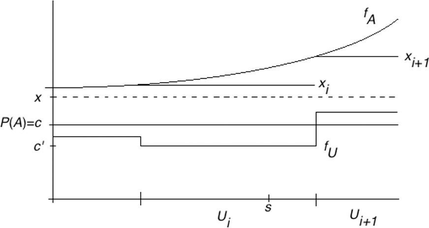
I will now return to the proof when  is infinite. This part of the proof will proceed by contradiction. Figure A1 will help keep track of the relevant values that are introduced.
Figure A1.

So assume that there is  such that
 for all s. (The dual case with
 such that
 for all s works similarly.) Let
 . Let
 . By Immodesty, ε is positive.
By Bounded Continuity, there are finitely many values  such that
 and
 . Let
 be the set of s such that
 . (By refinement of the partition if necessary, we can ensure that any nonempty
 will have
 , since
 for all s.) Because
 is constant on each element of
 , each
 must be a union of members of
 . If
 is the partition into the
 , then this means that
 is a coarsening of the partition
 .
Let  be a
 -available plan with minimal expected inaccuracy. Since
 is a finite partition, the finite part of this proof establishes that there is an s with
 . Let
 be the element of
 containing s, and let
 , so that
 for all s in
 . By the observation made after proving the finite version, we can ensure that
 . Thus, by the Ratio Analysis result, we see that
 . Let
 be the function that agrees with
 outside of
 and agrees with
 inside
 .
Now consider the set  of all
 -available functions that agree with
 outside
 . Note that
 and
 are both in
 . (The term
 is not
 -available, but it is
 -available.) I will also consider the function
 , which agrees with
 outside of
 and takes on the value
 for all s in
 . By linearity of expectations,

Because all of these functions are identical for s in  , their total expected inaccuracy will depend only on
 .
Because  and
 for all s in
 , we can see that

and

But we observed earlier that  , and thus since P is a probability function,
 , so we have

and

Since  , our two lemmas together tell us that
 . Thus, the expected inaccuracy of
 is at least
 greater than the expected inaccuracy of
 .
But for any s in  , the inaccuracy of
 on s is within ε of the inaccuracy of
 on s (because
 is always between
 and
 , which are chosen to make sure that regardless of whether A is true or false, the inaccuracy of any value in this range is within ε of the inaccuracy of any other value in this range—this is the one use of Monotonicity). Thus, the expected inaccuracy of
 is within
 of the expected inaccuracy of
 , which means that the expected inaccuracy of
 must be greater than the expected inaccuracy of
 .
Thus, since  and
 agree outside of
 , we see that the expected inaccuracy of
 is greater than the expected inaccuracy of
 , which contradicts the assumption that
 had minimal expected inaccuracy of any
 -available plan. Thus, the original assumption that there is x with
 and
 for all s must be false, which proves one direction of the inequality. The other direction is proven by the corresponding argument with all inequalities reversed. QED
Remark: if  differs from
 only on a set of probability 0, then the expected inaccuracy of both plans is the same, so that one has minimal expected inaccuracy if and only if the other does. Therefore, as a corollary, we have that for any
 , the set of s with
 must have nonzero probability—otherwise we could find an
 that also has minimal expected inaccuracy but violates the conclusion of the theorem.
Expectation Theorem. If for all propositions A in  the conditions of the Interval Theorem hold, and for each s,
 is a probability function (so that
 for all A,
 , and
 whenever A and B are disjoint), then for all A,
 .
Proof. This is a straightforward consequence of the Interval Theorem together with theorem 1 of Dubins (Reference Dubins1975), which states that an expectation is conglomerable if and only if it is disintegrable. The Interval Theorem shows that the expectation here is conglomerable, and the conclusion of this theorem is the claim that the expectation is disintegrable. QED
 (because it is a sum of terms that are all 0) while the second says
 . For a case where both are wrong, let
 be a random variable that takes a different positive value in every state. Both stipulations say
 , even though it seems clear that its expected value should be positive.