1 Introduction
Plasma-based propulsion systems are beginning to challenge the monopole of chemical thrusters in space applications. The high specific impulse (which allows for a huge reduction in the propellant mass) and high thrust efficiency make the plasma thruster an attractive solution for space propulsion. At the state of the art, plasma propulsion devices, such as the ion engine and the Hall effect thruster (Goebel & Katz Reference Goebel and Katz2008), have proven to have good performance but exhibit some critical issues: (i) their lifetimes are limited by the erosion of the extracting grids and the ceramic walls; (ii) they need an external cathode for charge compensation. Recent advances in plasma-based propulsion systems have led to the development of helicon plasma thrusters (HPTs) (Manente et al. Reference Manente, Trezzolani, Magarotto, Fantino, Selmo, Bellomo, Toson and Pavarin2019), whose plasma-generation system is derived from high-density helicon plasma sources (Chen Reference Chen2015). HPTs are characterized by a long life (electrodes or neutralizers are not necessary in these thrusters), and a reduced cost in respect to ion and Hall effect thrusters.
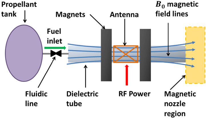
Helicon plasma thruster scheme.

In HPTs (see figure 1) we can distinguish between the production stage (i.e. the helicon source) and the acceleration stage, in which a magnetic nozzle (Ahedo & Merino Reference Ahedo and Merino2010) is employed to accelerate the magnetized plasma. The production stage is composed of a gas feeding system, a radio frequency (RF) antenna and magnetic coils. The neutral gas is injected into a dielectric cylinder and ionized through a RF antenna working in the MHz regime; the magnetic coils provide the magnetostatic field that improves the confinement of the plasma and allows the propagation of whistler waves (Chen & Arnush Reference Chen and Arnush1997). The acceleration stage is realized by means of the divergent magnetic field lines at the exhaust section, which provide a magnetic nozzle effect. HPTs are under study and development in some international research projects: the American VASIMR (Diaz Reference Diaz2000), where a high-power helicon source is coupled to a ion cyclotron resonance heating section to increase the specific impulse; the European HPH.COM (Pavarin et al.
Reference Pavarin, Ferri, Manente, Lucca Fabris, Trezzolani, Faenza, Tasinato, Rondini, Curreli and Melazzi2012) in which a low-power (
 ${\leqslant}$
100 W) system has been developed and SAPERE-STRONG (Trezzolani et al.
Reference Trezzolani, Manente, Selmo, Melazzi, Magarotto, Moretto, De Carlo, Pessana and Pavarin2017) that aims at the realization of a high-power (
 ${\geqslant}$
1 kW) propulsive system to be employed in a space tug. Other research centres involved in the study and development of HPTs are the Australian National University (Pottinger et al.
Reference Pottinger, Lappas, Charles and Boswell2011; Takahashi et al.
Reference Takahashi, Lafleur, Charles, Alexander, Boswell, Perren, Laine, Pottinger, Lappas and Harle2011), the Carlo III University of Madrid (Merino et al.
Reference Merino, Navarro, Casado, Ahedo, Gómez, Ruiz, Bosch and del Amo2015), Tokyo University (Kuwahara et al.
Reference Kuwahara, Koyama, Otsuka, Ishii, Ishii, Fujitsuka, Waseda and Shinohara2014; Shinohara et al.
Reference Shinohara, Nishida, Tanikawa, Hada, Funaki and Shamrai2014), the Tohoku University (Takahashi, Komuro & Ando Reference Takahashi, Komuro and Ando2015), the Massachusetts Institute of Technology (Batishchev Reference Batishchev2009), the Michigan Institute of Technology (Sheehan et al.
Reference Sheehan, Collard, Ebersohn and Longmier2015) and Washington University (Ziemba et al.
Reference Ziemba, Carscadden, Slough, Prager and Winglee2005).
In HPTs the propulsive figures of merit depend on the plasma parameters (e.g. plasma density and electron temperature) inside the helicon source. Plasma generation is mainly driven by the power deposited by the RF antenna into the source and the plasma transport therein. Therefore we need theoretical and numerical models of the wave propagation, and ultimately of the power deposition, to perform the design and optimization of HPTs. Many works tackle the power deposition by assuming the confinement magnetostatic field to be purely axial and uniform; however, helicon sources applied in actual HPTs can depart from this assumption due to dimension, mass and power budget limitations.
Many works on helicon sources have studied the physics of wave propagation and of power deposition. Main findings for uniform plasma sources are: (i) two coupled whistler waves, namely the helicon and Trivelpiece–Gould waves (Chen & Arnush Reference Chen and Arnush1997), propagate within the source; (ii) the power deposition occurs mainly at the edge of the plasma cylinder, where the Trivelpiece–Gould waves are damped by collisional processes (Chen & Blackwell Reference Chen and Blackwell1999). The influence of plasma non-uniformity has been widely investigated in both theoretical (Krämer Reference Krämer1999; Breizman & Arefiev Reference Breizman and Arefiev2000) and numerical (Mouzouris & Scharer Reference Mouzouris and Scharer1996; Chen et al. Reference Chen, Arefiev, Bengtson, Breizman, Lee and Raja2006) works. Less effort has been paid to studying the influence of non-uniform magnetostatic fields on the wave propagation. A series of experimental works have been carried out in order to understand the enhancement of power deposited when the helicon source is operating in a non-uniform magnetic field. However, in all these works, the data interpretation was based on simplified wave propagation models: in Braginskii, Vasileva & Kovalev (Reference Braginskii, Vasileva and Kovalev2001) a dispersion relation that does not account for magnetic field non-homogeneity has been adopted. In Virko et al. (Reference Virko, Shamrai, Virko and Kirichenko2004) a simplified plane wave model, that can account for radial components of the magnetic field but not for inhomogeneities has been used. In Guo et al. (Reference Guo, Scharer, Mouzouris and Louis1999) a comparative numerical analysis has been performed accounting only for the axial component of the magnetic confinement field. A detailed experimental campaign has been carried out in Lafleur, Charles & Boswell (Reference Lafleur, Charles and Boswell2010, Reference Lafleur, Charles and Boswell2011) in order to analyse the performances of a piglet helicon reactor operating in a non-uniform magnetic field. In Lafleur et al. (Reference Lafleur, Charles and Boswell2011), the authors found that the axial distance over which waves propagate can be controlled through magnetic field strength and geometry, the latter being critical in the region near the exit of the source; nonetheless, the results have been interpreted by relying on the helicon dispersion relation that does not account for a non-uniform magnetic field. An experimental and numerical work on the helicon waves propagation in a non-uniform magnetic field has been carried out by Chang et al. (Reference Chang, Hole, Caneses, Chen, Blackwell and Corr2012); they found that the helicon wave has weaker attenuation away from the antenna in a focused magnetic field than in a uniform field. The numerical tool employed in Chang et al. (Reference Chang, Hole, Caneses, Chen, Blackwell and Corr2012) cannot deal with a generic magnetic field geometry, since the radial component of the magnetic field has been assumed to have axial expansion. Helicon sources working in non-uniform fields have been studied also in purely numerical works (Kinder & Kushner Reference Kinder and Kushner2001; Bose, Govindan & Meyyappan Reference Bose, Govindan and Meyyappan2003). However, the authors analysed only one magnetic field geometry: this prevents any insight into the influence of magnetic field components in the source performance, and ultimately on the power deposition.
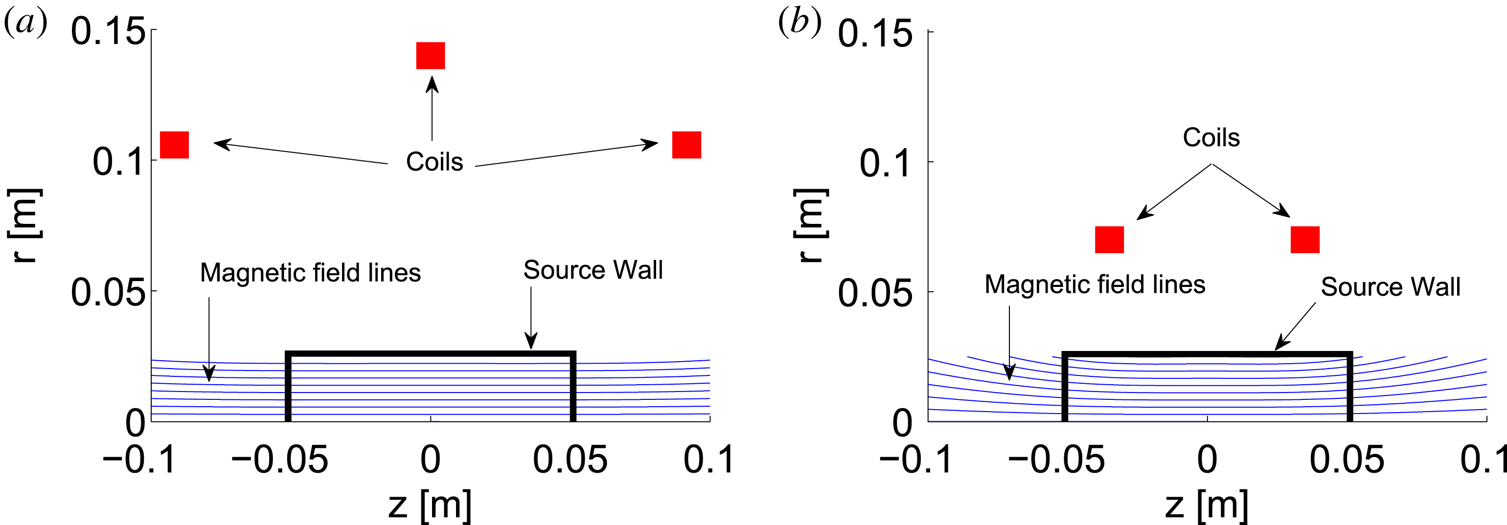
We have numerically studied how the geometry of the confinement magnetic field affects the power deposition in a cylindrical helicon source. We have solved the wave propagation by means of two electromagnetic (EM) solvers, namely: (i) plaSma Padova Inhomogeneous Radial Electromagnetic solver (SPIREs) (Melazzi et al. Reference Melazzi, Curreli, Manente, Carlsson and Pavarin2012), a mono-dimensional finite-difference frequency-domain code, and (ii) Advanced coDe for Anisotropic Media and ANTennas (ADAMANT) (Melazzi & Lancellotti Reference Melazzi and Lancellotti2014), a full-wave three-dimensional (3-D) tool based on the method of moments. We have computed the deposited power spectrum along the radial direction and for different propagating modes, with SPIREs. Instead, ADAMANT has been adopted to accurately calculate the 3-D power deposition profile into the plasma. Moreover, both codes have been exploited to compute the antenna impedance. We have analysed two configurations of the magnetostatic field, namely those produced by Maxwell coils and Helmholtz coils. The former set-up provides an almost axial and uniform magnetostatic field, while the latter introduces non-negligible gradients of the magnetostatic field along the radial and axial directions (see figure 2). In particular, similar magnetic geometries have been adopted in actual experiments: in Ziemba et al. (Reference Ziemba, Carscadden, Slough, Prager and Winglee2005) the magnetostatic field is produced by two Helmholtz coils, while in both Pottinger et al. (Reference Pottinger, Lappas, Charles and Boswell2011), Merino et al. (Reference Merino, Navarro, Casado, Ahedo, Gómez, Ruiz, Bosch and del Amo2015) a three electromagnet configuration has been adopted.
Draft of the magnetic field geometry generated by: (a) Maxwell coils, (b) Helmholtz coils.

The paper is structured as follows: in § 2, we have described the numerical methodology; in § 3 we have discussed the sensitivity analysis conducted to verify the accuracy of both codes; the results obtained with SPIREs and ADAMANT are reported respectively in § 4 and § 5; finally in § 6, conclusions are drawn.
2 Methodology
We have modelled the helicon source as a plasma cylinder surrounded by a RF antenna and enclosed inside a conducting tube. Moreover, we have assumed the presence of a generic distribution of coaxial coils that generate the actual confinement magnetostatic field. The latter is axisymmetric with radial (
 $B_{0r}$
) and axial (
 $B_{0z}$
) components that depends on the radial (
 $r$
) and axial (
 $z$
) position within the source. Since we want to focus our attention on the influence of the magnetostatic field geometry on the power deposition, we have assumed uniform plasma density
 $n$
, electron temperature
 $T_{e}$
and neutral pressure
 $p_{0}$
. We relied (i) on SPIREs to calculate the antenna impedance
 $Z$
, and the radial profile of the deposited power spectrum
 $P_{r}$
, and (ii) on ADAMANT for
 $Z$
and the 3-D power deposition profile
 ${\mathcal{E}}_{\text{pow}}$
.
It is worth specifying why we adopted two different EM solvers to study a helicon source. SPIREs has been exploited to preliminarily evaluate the effect of the non-uniform magnetostatic field on the power spectrum. The latter provides a very unique physical insight into the problem at hand, making it possible to isolate the contribution given by each propagative mode. Nonetheless, SPIREs is a 1-D radial solver, so its output depends only on the value of the magnetostatic field and of the plasma parameters in a single axial section. This means that: (i) effects of radial gradients can be directly calculated, (ii) effects of axial gradients can be evaluated by only comparing the results of SPIREs runs in different axial sections. Therefore, we have verified the reliability of SPIREs by means of the ADAMANT code, which has been exploited to accurately calculate
 ${\mathcal{E}}_{\text{pow}}$
. Nonetheless, ADAMANT is not suitable for spectral analyses, so the contributions given by each propagative mode cannot be separated. In conclusion, we opted for a combined strategy which relies on both the SPIREs and ADAMANT codes.
2.1 SPIREs
The governing equations solved in SPIREs are the Faraday and the Ampere–Maxwell laws (Jackson Reference Jackson1999). Therefore, assuming a harmonic dependence to time and space in the form of
 $\exp \text{i}(m\unicode[STIX]{x1D703}+k_{z}z-\unicode[STIX]{x1D714}t)$
for both fields and sources, we obtain
 $$\begin{eqnarray}\displaystyle & \displaystyle \unicode[STIX]{x1D735}\times \tilde{\boldsymbol{E}}=\text{i}\unicode[STIX]{x1D714}\tilde{\boldsymbol{B}} & \displaystyle\end{eqnarray}$$
 $$\begin{eqnarray}\displaystyle & \displaystyle \unicode[STIX]{x1D735}\times \tilde{\boldsymbol{B}}=-\text{i}\unicode[STIX]{x1D714}\tilde{\boldsymbol{D}}+\tilde{\boldsymbol{J}}. & \displaystyle\end{eqnarray}$$
 $\tilde{\boldsymbol{J}}$
has been assumed on the antenna in accordance with the thin wire approximation (Mouzouris & Scharer Reference Mouzouris and Scharer1996). The electric field
 $\tilde{\boldsymbol{E}}$
and the magnetic induction
 $\tilde{\boldsymbol{B}}$
are related respectively to the electric displacement
 $\tilde{\boldsymbol{D}}$
and the magnetic field
 $\tilde{\boldsymbol{H}}$
through the constitutive relations
 $$\begin{eqnarray}\displaystyle & \displaystyle \tilde{\boldsymbol{B}}=\unicode[STIX]{x1D707}_{0}\tilde{\boldsymbol{H}} & \displaystyle\end{eqnarray}$$
 $$\begin{eqnarray}\displaystyle & \displaystyle \tilde{\boldsymbol{D}}=\unicode[STIX]{x1D73A}\tilde{\boldsymbol{E}}, & \displaystyle\end{eqnarray}$$
 $\unicode[STIX]{x1D707}_{0}$
is the vacuum permeability, and
 $\unicode[STIX]{x1D73A}$
is the Stix tensor (Stix Reference Stix1962). The latter is formulated in order to account for a general magnetostatic field geometry, namely
 $$\begin{eqnarray}\unicode[STIX]{x1D73A}=\left[\begin{array}{@{}ccc@{}}K_{1} & K_{4} & K_{5}\\ -K_{4} & K_{2} & K_{6}\\ K_{5} & -K_{6} & K_{3}\\ \end{array}\right]\!.\end{eqnarray}$$
The definitions of complex coefficients
 $K_{n}(n=1\,\ldots \,6)$
can be found in Swanson (Reference Swanson2012). It is worth highlighting that such a formulation for the EM problem represents a reasonable approximation of a magnetized plasma unless nonlinear effects of wave–particle interaction become relevant (Melazzi et al.
Reference Melazzi, Curreli, Manente, Carlsson and Pavarin2012).
In general: (i)
 $m$
(i.e. the azimuthal wavenumber) is known from the antenna geometry (Mouzouris & Scharer Reference Mouzouris and Scharer1996), (ii)
 $\unicode[STIX]{x1D714}$
(i.e. the oscillation frequency) depends on the antenna feeding system, (iii)
 $k_{z}$
(i.e. the axial mode number) depends on the plasma parameters (e.g. plasma density and electron temperature) and magnetostatic field geometry. To evaluate the propagative
 $k_{z}$
we have resorted to the general dispersion relation that reads
 $$\begin{eqnarray}Kk_{r}^{4}+\unicode[STIX]{x1D6EC}k_{r}^{3}+Mk_{r}^{2}+Nk_{r}+\unicode[STIX]{x1D6F1}=0,\end{eqnarray}$$
where
 $k_{r}$
is the propagative wavenumber in the radial direction, whereas the coefficients
 $K$
,
 $\unicode[STIX]{x1D6EC}$
,
 $M$
,
 $N$
,
 $\unicode[STIX]{x1D6F1}$
depend on
 $k_{z}$
,
 $m$
,
 $B_{0r}$
,
 $B_{0z}$
and plasma parameters. The expression of these coefficients can be found in Cardinali et al. (Reference Cardinali, Melazzi, Manente and Pavarin2014). Equation (2.4) is employed as follows: we impose
 $m$
,
 $B_{0r}$
,
 $B_{0z}$
, and we solve the dispersion relation for an interval of
 $k_{z}$
; if the calculated
 $k_{r}$
is real than the wave is propagative, otherwise not. Subsequently, we solve equations (2.1) for each
 $m$
,
 $k_{z}$
propagative couple and we obtain the radial profiles of electric field
 $\tilde{\boldsymbol{E}}_{P}$
, and plasma current
 $\tilde{\boldsymbol{J}}_{P}$
spectra. Therefore we can calculate the radial profile of the deposited power spectrum
 $$\begin{eqnarray}P_{r}={\textstyle \frac{1}{2}}\tilde{\boldsymbol{E}}_{P}\boldsymbol{\cdot }\tilde{\boldsymbol{J}}_{P}.\end{eqnarray}$$
Moreover, the total power deposited inside the discharge can be computed as (Mouzouris & Scharer Reference Mouzouris and Scharer1996)
 $$\begin{eqnarray}Pw={\textstyle \frac{1}{2}}\int \boldsymbol{E}_{P}\boldsymbol{\cdot }\boldsymbol{J}_{P}\,\text{d}V,\end{eqnarray}$$
where the integration is performed on the overall discharge volume, and
 $\boldsymbol{E}_{P}$
and
 $\boldsymbol{J}_{P}$
are obtained anti-transforming respectively
 $\tilde{\boldsymbol{E}}_{P}$
and
 $\tilde{\boldsymbol{J}}_{P}$
(Melazzi et al.
Reference Melazzi, Curreli, Manente, Carlsson and Pavarin2012). Therefore the antenna impedance is calculated as
 $$\begin{eqnarray}Z=\frac{2}{|I_{A}|^{2}}Pw,\end{eqnarray}$$
where
 $I_{A}$
is the intensity of the current imposed on the antenna.
In passing, we recall that, in SPIREs, equations (2.1) have been discretized into a set of linear algebraic equations by means of the finite-difference method implemented on a radial Yee mesh. The resultant linear system (which is sparse, non-symmetric and with non-zero elements in complex domain) has been resolved using the MUltifrontal Massively Parallel Solver (MUMPS) (Amestoy et al. Reference Amestoy, Duff, LExcellent and Koster2007) with a lower-upper (LU) factorization. For further details on the numerical scheme adopted in SPIREs, the reader is referred to Melazzi et al. (Reference Melazzi, Curreli, Manente, Carlsson and Pavarin2012).
2.2 ADAMANT
In ADAMANT the wave propagation is solved in a helicon plasma source assuming the metallic antenna to be a perfect electric conductor and the plasma to be a dielectric medium described by means of the Stix tensor (see equation (2.3)). ADAMANT solves the unknown current on the antenna
 $\boldsymbol{J}_{A}$
and the polarization current on the plasma volume
 $\boldsymbol{J}_{P}$
. From these quantities, the antenna impedance
 $Z$
and the 3-D power deposition profile into the plasma
 ${\mathcal{E}}_{\text{pow}}$
can be derived.
Enforcing the boundary condition for the total tangential electric field on the antenna surface (Rothwell & Cloud Reference Rothwell and Cloud2018) we obtain
 $$\begin{eqnarray}[\boldsymbol{E}_{AA}^{S}+\boldsymbol{E}_{AP}^{S}+\boldsymbol{E}_{AA}^{i}]|_{\text{tan}}=0.\end{eqnarray}$$
Instead, expressing the total electric field in the plasma volume as the sum of antenna and plasma contributions yields
 $$\begin{eqnarray}\boldsymbol{E}_{P}=\boldsymbol{E}_{PA}^{S}+\boldsymbol{E}_{PP}^{S}.\end{eqnarray}$$
Specifically,
 $\boldsymbol{E}_{AA}^{S}$
(
 $\boldsymbol{E}_{AP}^{S}$
) represents the secondary electric field radiated by
 $\boldsymbol{J}_{A}$
(
 $\boldsymbol{J}_{P}$
) onto the antenna. At the same time
 $\boldsymbol{E}_{PA}^{S}$
(
 $\boldsymbol{E}_{PP}^{S}$
) denotes the secondary electric field produced by
 $\boldsymbol{J}_{A}$
(
 $\boldsymbol{J}_{P}$
) within the plasma volume. The impressed
 $\boldsymbol{E}_{AA}^{i}$
field is given from the voltage-gap approximation Balanis (Reference Balanis2016). Moreover,
 $\boldsymbol{E}_{P}$
is the electric field on the plasma volume. The equations which link the secondary fields to their sources can be found in Melazzi & Lancellotti (Reference Melazzi and Lancellotti2014).
In particular, from the knowledge of
 $\boldsymbol{J}_{A}$
and
 $\boldsymbol{J}_{P}$
, the antenna impedance is calculated as (Melazzi & Lancellotti Reference Melazzi and Lancellotti2014, equation (11))
 $$\begin{eqnarray}Z=\frac{I_{A}}{V_{G}},\end{eqnarray}$$
where
 $V_{G}$
is the intensity of the voltage imposed (by means of the voltage-gap approximation) on the antenna port, and
 $I_{A}$
is the current therein. Moreover, we obtain the 3-D power deposition profile in the plasma from (Melazzi & Lancellotti Reference Melazzi and Lancellotti2014, equation (12))
 $$\begin{eqnarray}{\mathcal{E}}_{\text{pow}}={\textstyle \frac{1}{2}}\boldsymbol{E}_{P}\boldsymbol{\cdot }\boldsymbol{J}_{P}.\end{eqnarray}$$
Finally, it is worth highlighting that the method of moments in Galerkin’s form Peterson, Ray & Mittra (Reference Peterson, Ray and Mittra1998) is adopted to turn the governing equations (2.8) and (2.9) into a linear algebraic system. For this purpose, we model the antenna with a triangular surface mesh and the plasma volume with a tetrahedral mesh. The resulting linear system is solved with the LU factorization (Amestoy et al. Reference Amestoy, Duff, LExcellent and Koster2007). For further details on the numerical scheme adopted in ADAMANT, the reader is referred to Melazzi & Lancellotti (Reference Melazzi and Lancellotti2014).
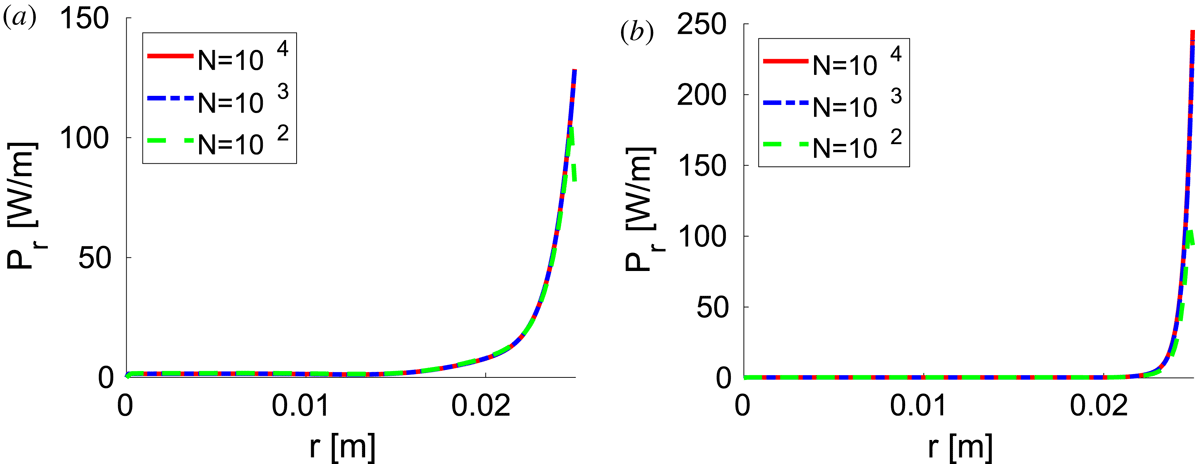
Real part of the power spectrum
 $P_{r}$
calculated with SPIREs for different mesh sizes, namely number of radial nodes
 $N$
ranging from
 $10^{2}$
up to
 $10^{4}$
. Magnetostatic field generated by Helmholtz coils, uniform plasma of density
 $n=10^{18}~\text{m}^{-3}$
, (a) average magnetostatic field on the central axial section
 $B_{0}=200$
G, and axial wavenumber
 $k_{z}=19.40~\text{m}^{-1}$
, (b)
 $B_{0}=1000$
G and
 $k_{z}=7.36~\text{m}^{-1}$
.

3 Numerical accuracy
The accuracy of both SPIREs and ADAMANT has been investigated respectively in Melazzi et al. (Reference Melazzi, Curreli, Manente, Carlsson and Pavarin2012) and Melazzi & Lancellotti (Reference Melazzi and Lancellotti2014) if the plasma is surrounded by a uniform magnetostatic field. Therefore we have performed a similar analysis in order to account for the effect of a non-uniform magnetostatic field. To this end, we have considered a cylindrical helicon plasma source of radius
 $R=0.025$
m, length
 $L=0.10$
m and filled with a uniform plasma of density
 $n=10^{18}~\text{m}^{-3}$
, temperature
 $T_{e}=3$
eV and neutral pressure
 $p_{0}=15$
mTorr. The system is driven by a loop antenna (azimuthal mode
 $m=0$
) located in the centre of the discharge (
 $z=0$
m) and excited at a frequency
 $f=13.56$
MHz.
First, a sensitivity analysis has been conducted on SPIREs in order to evaluate the influence of the mesh size on the real part of the power spectrum
 $P_{r}$
. In particular we have considered the system surrounded by a magnetic geometry produced by Helmholtz coils (see figure 2). Two cases have been considered: (i) average magnetostatic field on the central axial section
 $B_{0}=200$
G, and axial wavenumber
 $k_{z}=19.40~\text{m}^{-1}$
(see figure 3
a), (ii)
 $B_{0}=1000$
G and
 $k_{z}=7.36~\text{m}^{-1}$
(see figure 3
b). Grids of three different sizes have been adopted, namely number of radial nodes
 $N=10^{2}$
,
 $N=10^{3}$
and
 $N=10^{4}$
. In both cases, increasing
 $N$
above
 $10^{3}$
does not produce any significant effect (lower than 1 %) on the
 $P_{r}$
profile. Also for other wavenumbers, or if the discharge is surrounded by the magnetostatic field produced by Maxwell coils (see figure 2), similar results hold true (not reported for the sake of brevity). Therefore, in the following, grids composed of
 $N=10^{3}$
nodes have been adopted.
Second, we have conducted a sensitivity analysis on the unstructured 3-D plasma mesh of ADAMNT. The real part of the antenna impedance
 $\text{Re}(Z)$
has been evaluated as a function of the number of tetrahedra which constitute the plasma mesh
 $N_{A}$
. We have considered the system to be surrounded by a magnetic field of intensity
 $B_{0}=200$
G and produced by Helmholtz coils. Three different grids have been evaluated, namely characterized by
 $N_{A}=2000$
,
 $N_{A}=4500$
and
 $N_{A}=7000$
. Increasing
 $N_{A}$
above
 $4500$
do not produce significant changes (lower than 1 %) to the value of
 $Z$
computed (see Table 1). Also if the magnetostatic field is produced by Maxwell coils similar results hold true (not reported for the sake of brevity). Therefore, in the rest of this work a 3-D plasma mesh composed of
 $N_{A}=4500$
tetrahedra has been adopted.
Real part of the antenna impedance
 $\text{Re}(Z)$
calculated as the number of tetrahedra of the plasma mesh of ADAMANT (
 $N_{A}$
) varies from
 $2000$
up to
 $7000$
. Uniform plasma of density
 $n=10^{18}~\text{m}^{-3}$
, and magnetostatic field generated by Helmholtz coils of intensity
 $B_{0}=200$
G.

Third, the results of SPIREs and ADAMANT have been compared. The real part of the antenna impedance
 $\text{Re}(Z)$
has been adopted to evaluate the consistency between the two codes. The system is surrounded by three different magnetic geometries, namely a uniform field, that generated by Maxwell coils and that generated by Helmholtz coils (see table 2). The average magnetostatic field on the central axial section is
 $B_{0}=200$
G. The mesh of SPIREs consists of
 $N=10^{3}$
equidistant radial nodes; for ADAMANT, the plasma volume is meshed with
 $N_{A}=4500$
tetrahedra. The values of
 $\text{Re}(Z)$
calculated with the two solvers differ by approximately 5 %. Moreover, both SPIREs and ADAMANT predict that
 $\text{Re}(Z)$
is almost equal in the uniform and Maxwell coil configurations, while it decreases by approximately 5 % in the Helmholtz coli case. It is worthwhile mentioning that the two codes are not in general expected to predict exactly the same results. In fact, SPIREs is a 1-D tool whereas ADAMANT solves Maxwell’s equations in a 3-D domain. Moreover the former relies on the spectral representation of the assumed antenna current, while the latter computes said current. So accounting for these different modelling, we can conclude that the two codes are consistent.
Comparison between the real part of the antenna impedance
 $\text{Re}(Z)$
calculated with SPIREs and ADAMANT for three different magnetic geometries, namely uniform field, that generated by Maxwell coils and that generated by Helmholtz coils. Uniform plasma of density
 $n=10^{18}~\text{m}^{-3}$
, and magnetostatic field of intensity
 $B_{0}=200$
G.

4 Mono-dimensional analysis
We have studied the power deposition in a helicon source of radius
 $R=0.025$
m, length
 $L=0.10$
m and driven by a loop antenna (i.e. azimuthal wavenumber
 $m=0$
) located in the centre of the discharge (
 $z=0$
m) and excited at a frequency
 $f=13.56$
MHz; the current flowing is
 $I=1$
A. We have analysed the magnetostatic field generated by two coil configurations, namely Maxwell coils and Helmholtz coils (see figure 2). The average magnetostatic field on the central axial section
 $B_{0}$
has been studied in the range from 250 G up to 1000 G. Since we want to investigate the influence of the magnetostatic field geometry on the power deposition, we have assumed that the plasma is uniform. We have analysed plasma density
 $n$
from
 $10^{17}~\text{m}^{-3}$
up to
 $10^{19}~\text{m}^{-3}$
, pressure of neutral background
 $p_{0}=15$
mTorr and electron temperature
 $T_{e}=3$
eV. We have studied the Maxwell and the Helmholtz coil configurations in three selected cases, namely: (i) low density
 $n=10^{17}~\text{m}^{-3}$
and low magnetic field
 $B_{0}=250$
G, hereinafter referred to as case low; (ii) medium density
 $n=10^{18}~\text{m}^{-3}$
and medium magnetic field
 $B_{0}=500$
G, referred to as case medium; (iii) high density
 $n=10^{19}~\text{m}^{-3}$
and high magnetic field
 $B_{0}=1000$
G, referred to as case high.
4.1 Maxwell coils
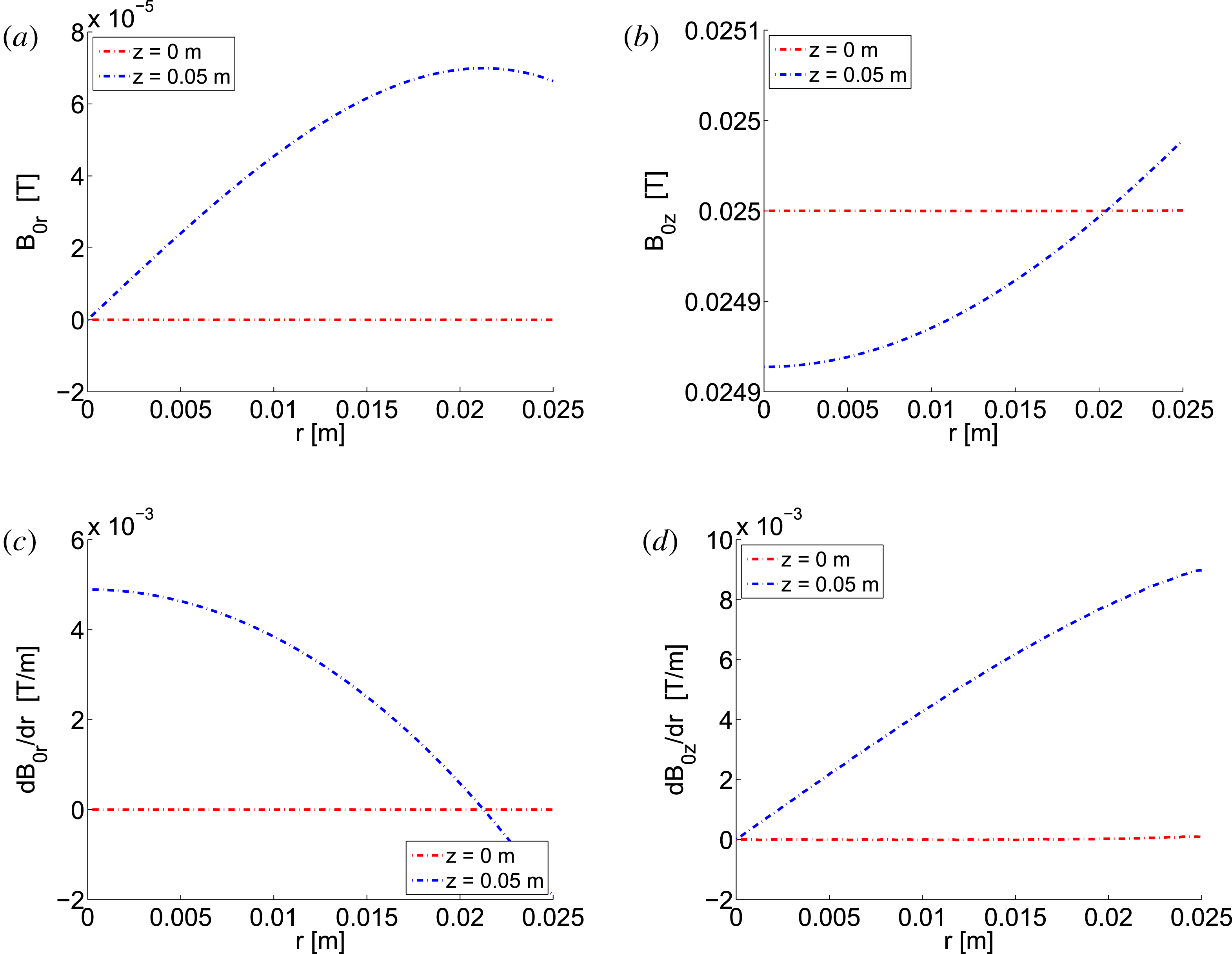
In figure 4 we have reported the radial (
 $B_{0r}$
) and axial (
 $B_{0z}$
) components of the magnetostatic field, along with their derivatives in the radial direction
 $r$
. Data are depicted in two axial sections, namely the centre of the source (
 $z=0$
m) and the boundary (
 $z=0.05$
m). We have reported only Case Low because the other two cases can be easily derived by rescaling the intensity of the field. In the Maxwell coil configuration, the field departs very mildly from the uniform case: the ratio
 $B_{0r}/B_{0z}$
is lower than 1 % everywhere inside the source.
Maxwell coil configuration in case low: confinement magnetic field along the radial direction
 $r$
at two axial sections, namely
 $z=0$
m (centre of the discharge),
 $z=0.05$
m (boundary of the discharge). (a) Radial component (
 $B_{0r}$
), (b) axial component (
 $B_{0z}$
), (c) gradient of
 $B_{0r}$
along the radial direction, (d) gradient of
 $B_{0z}$
along the radial direction.

4.1.1 Case low
In figure 5, the real part of the power spectrum
 $P_{r}$
is depicted at
 $z=0$
m, and
 $z=0.05$
m. In both sections
 $P_{r}$
is peaked in correspondence with the outer radius of the discharge. In particular, at
 $z=0$
m and for opposite values of
 $k_{z}$
, the power spectrum profiles are perfectly superposed (see figure 5
a). This does not hold true as soon as a non-null
 $B_{0r}$
component is introduced, see figure 5(b) for
 $z=0.05$
m. Moreover, the total amount of power deposited in the discharge is related to the real part of the antenna impedance
 $\text{Re}(Z)$
(see equation (2.7)), whose value is
 $\text{Re}(Z)=0.0299~\unicode[STIX]{x03A9}$
. It is worth highlighting that, assuming a uniform magnetostatic field, we would have obtained
 $\text{Re}(Z)=0.0300~\unicode[STIX]{x03A9}$
. Therefore, we can conclude that the influence of the magnetostatic field non-homogeneities (i) on the power spectrum is mild, and (ii) on the overall amount of power deposited is negligible.
Maxwell coil configuration in case low:
 $n=10^{17}~\text{m}^{-3}$
,
 $B_{0}=250$
G. Real part of the power spectrum (
 $P_{r}$
) as a function of the radial position (
 $r$
), evaluated for different axial wavenumbers (
 $k_{z}$
). (a) Centre of the discharge
 $z=0$
m; (b) boundary of the discharge
 $z=0.05$
m.

4.1.2 Case medium
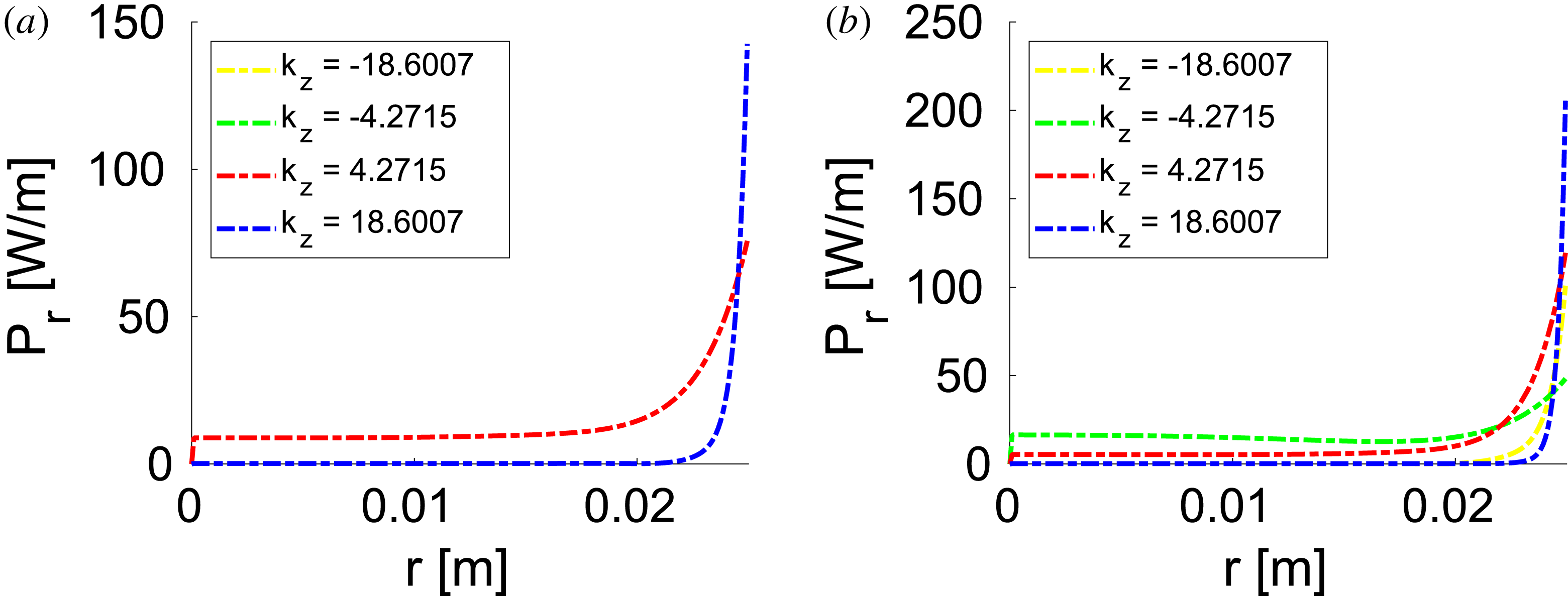
In figure 6, the real part of the power spectrum
 $P_{r}$
is depicted at
 $z=0$
m, and
 $z=0.05$
m. The power spectrum profiles present the same features as case low, namely: (i) peaked on the outer radius of the discharge, and (ii) no longer superposed for opposite
 $k_{z}$
if the
 $B_{0r}$
component is non-null. Moreover, the real part of the plasma impedance is respectively
 $\text{Re}(Z)=0.2475~\unicode[STIX]{x03A9}$
and
 $\text{Re}(Z)=0.2483~\unicode[STIX]{x03A9}$
considering a non-uniform or a uniform magnetostatic field. Therefore, also in this case the effects of the magnetostatic field inhomogeneities are: (i) mild on
 $P_{r}$
, and (ii) negligible in terms of total power deposited.
Maxwell coil configuration for case medium:
 $n=10^{18}~\text{m}^{-3}$
,
 $B_{0}=500$
G. Real part of the power spectrum (
 $P_{r}$
) as a function of the radial position (
 $r$
), evaluated for different axial wavenumbers (
 $k_{z}$
). (a) Centre of the discharge
 $z=0$
m; (b) boundary of the discharge
 $z=0.05$
m.

4.1.3 Case high
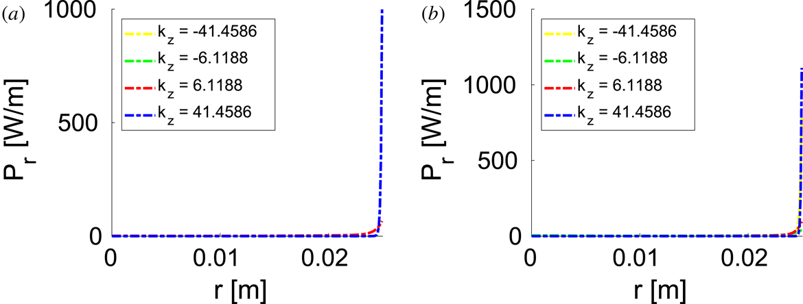
In figure 7, the real part of the power spectrum
 $P_{r}$
is presented at
 $z=0$
m, and
 $z=0.05$
m. As found in the previous cases, the power spectrum profiles are: (i) peaked on the outer radius of the discharge, and (ii) superposed for opposite
 $k_{z}$
only if the
 $B_{0r}$
component is null. The real part of the plasma impedance is respectively
 $\text{Re}(Z)=0.9338~\unicode[STIX]{x03A9}$
and
 $\text{Re}(Z)=0.9345~\unicode[STIX]{x03A9}$
considering a non-uniform or a uniform magnetostatic field. Therefore, the power deposition phenomenon is very mildly affected by the magnetostatic field inhomogeneities also in this case.
Maxwell coil configuration for case high:
 $n=10^{19}~\text{m}^{-3}$
,
 $B_{0}=1000$
G. Real part of the power spectrum (
 $P_{r}$
) as a function of the radial position (
 $r$
), evaluated for different axial wavenumbers (
 $k_{z}$
). (a) Centre of the discharge
 $z=0$
m; (b) boundary of the discharge
 $z=0.05$
m.

4.2 Helmholtz coils
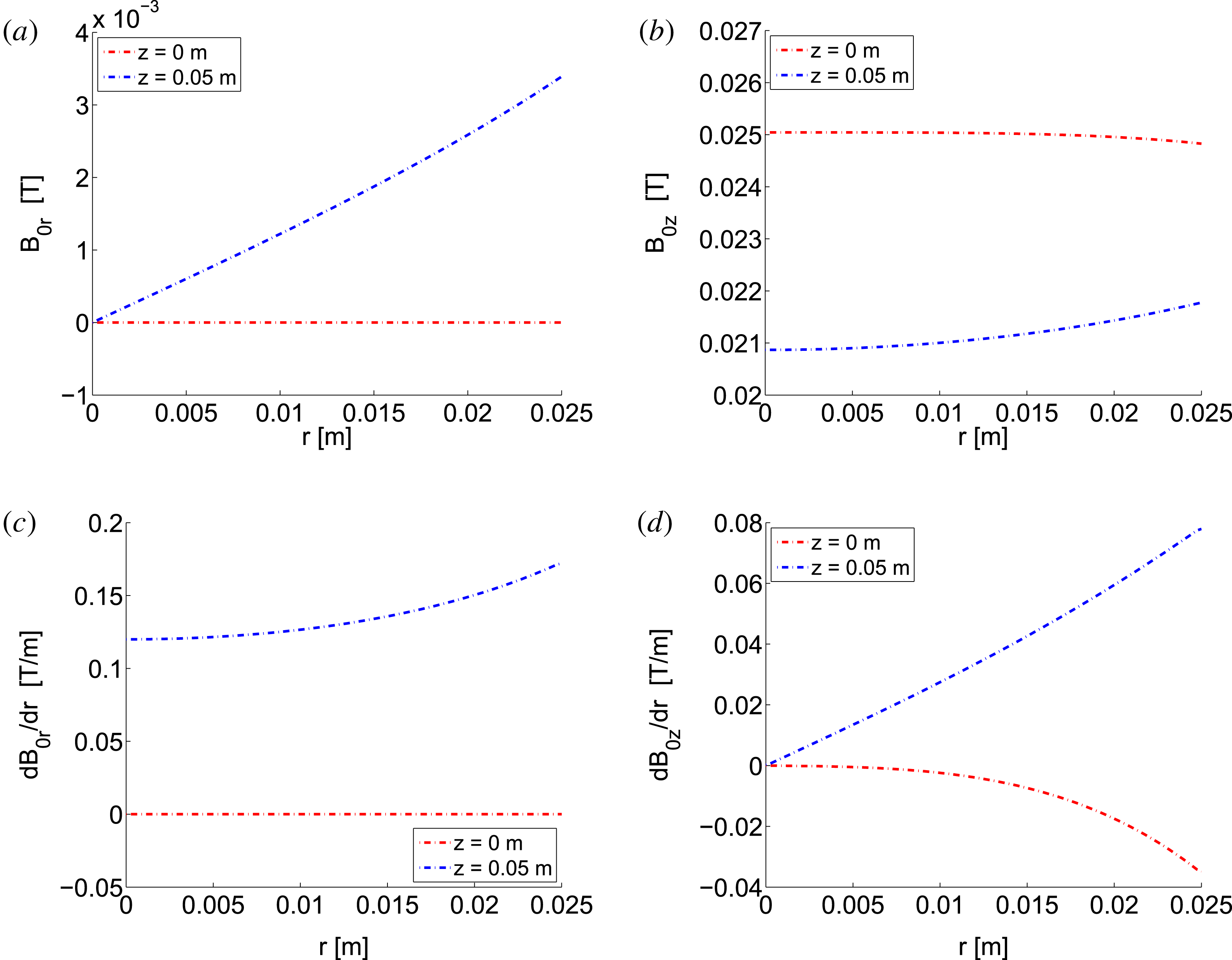
In figure 8 we have reported the radial (
 $B_{0r}$
) and axial (
 $B_{0z}$
) components of the magnetostatic field, along with their derivatives in the radial direction
 $r$
. Results are depicted at two axial sections, namely the centre of the source (
 $z=0$
m) and the boundary (
 $z=0.05$
m). We have reported only case low because the other two cases can be easily derived rescaling the intensity of the field. In the Helmholtz coil configuration, the ratio
 $B_{0r}/B_{0z}$
is up to 10 % within the discharge.
Helmholtz coil configuration in the low-magnetic-field case: confinement magnetic field along the radial direction
 $r$
at two axial sections, namely
 $z=0$
m (centre of the discharge),
 $z=0.05$
m (boundary of the discharge). (a) Radial component (
 $B_{0r}$
), (b) axial component (
 $B_{0z}$
), (c) gradient of
 $B_{0r}$
along the radial direction, (d) gradient of
 $B_{0z}$
along the radial direction.

4.2.1 Case low
At
 $z=0$
m, the real part of the power spectrum
 $P_{r}$
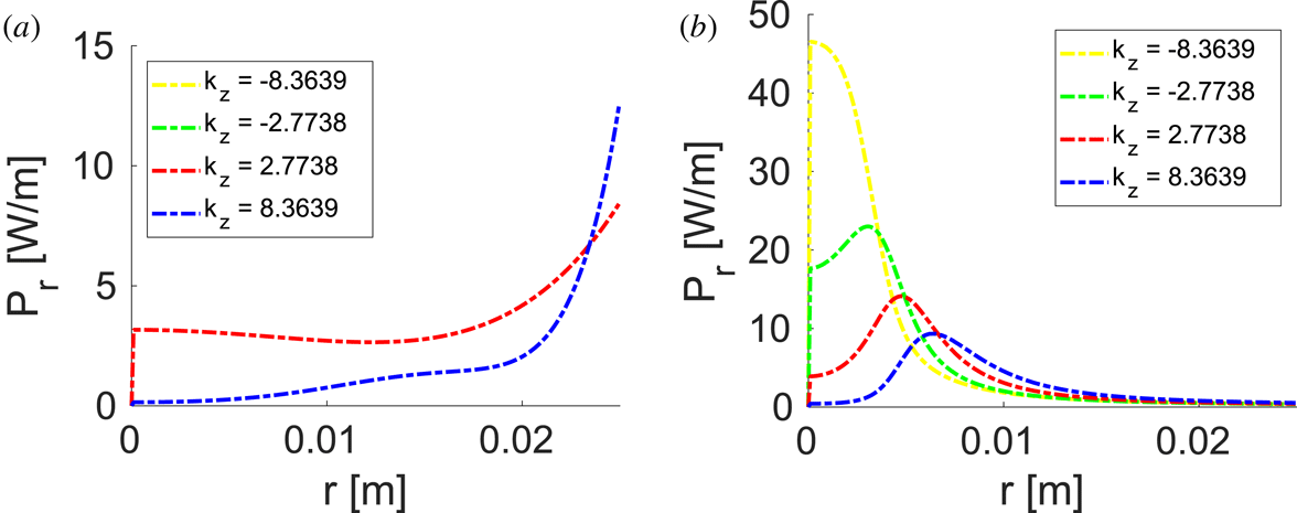
is peaked in correspondence with the outer radius of the discharge, as in the Maxwell coil configuration (compare figure 9
a and figure 5
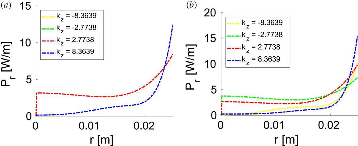
a). On the contrary at
 $z=0.05$
m,
 $P_{r}$
is peaked near the axis of the source (see figure 9
b). Moreover, the real part of the plasma impedance is equal to
 $\text{Re}(Z)=0.0255~\unicode[STIX]{x03A9}$
, which means a reduction of roughly 15 % in respect of the value obtained for the uniform field (
 $0.0300~\unicode[STIX]{x03A9}$
). It is worth highlighting that the ratio
 $B_{0r}/B_{0z}$
is of the order of 10 % at the boundary of the source. Therefore this relatively small departure from the perfectly axial magnetic geometry can have significant effects on both (i) the power spectrum, and (ii) the total amount of power deposited into the discharge.
Helmholtz coil configuration for case low. Real part of the power spectrum (
 $P_{r}$
) as a function of the radial position (
 $r$
), evaluated for different axial wavenumbers (
 $k_{z}$
). (a) Centre a of the discharge
 $z=0$
m; (b) boundary of the discharge
 $z=0.05$
m.

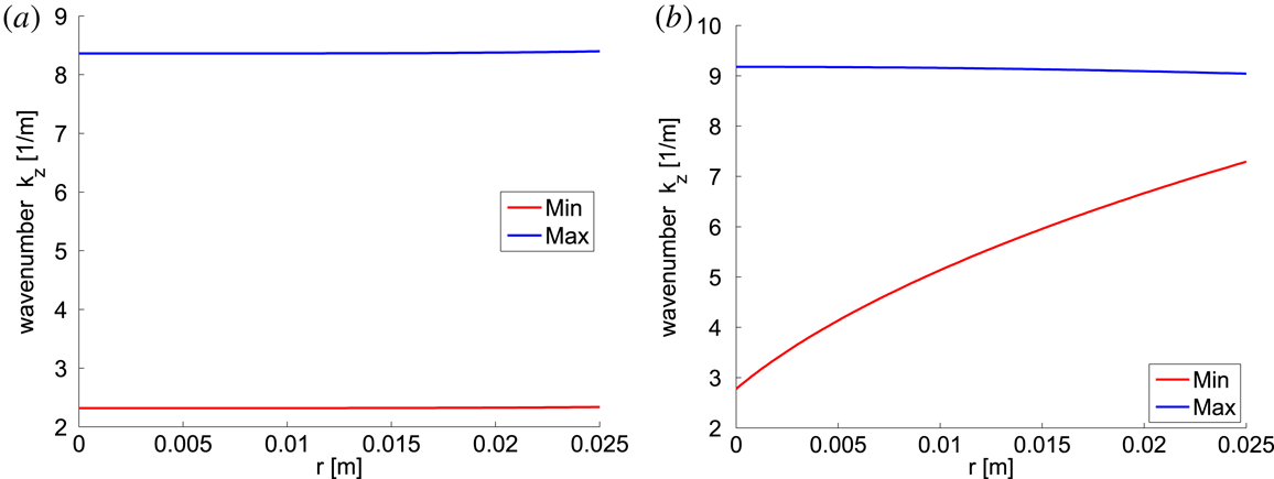
Helmholtz coil configuration for case low: interval of propagative EM waves, expressed in terms of axial wavenumber
 $k_{z}$
, along the radius of the discharge. The propagative interval is included between the minimum propagative
 $k_{z}$
(Min), and the maximum (Max). (a) Centre of the discharge
 $z=0$
m; (b) boundary of the discharge
 $z=0.05$
m.

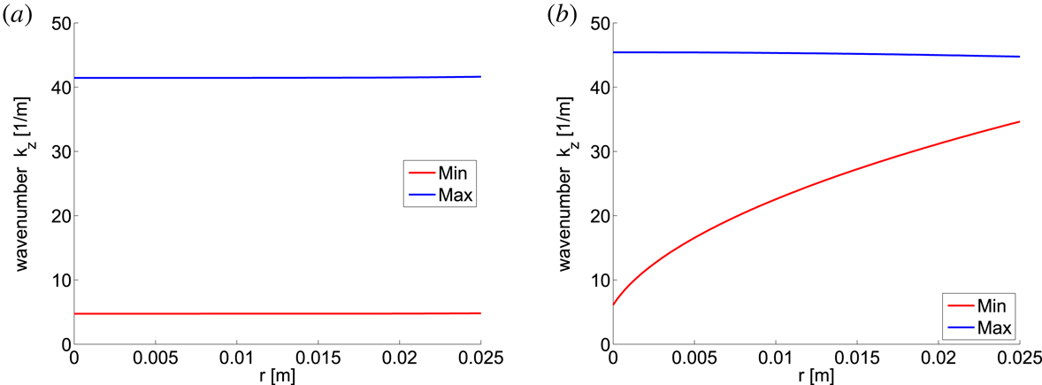
Moreover, the effects of the magnetostatic field inhomogeneities on the power deposition phenomenon can be interpreted by analysing the dispersion relation reported in (2.4) (Cardinali et al.
Reference Cardinali, Melazzi, Manente and Pavarin2014). In fact, in the centre of the discharge, where the magnetostatic field is almost homogeneous and axial, the interval of propagative EM waves (expressed in terms of axial wavenumber
 $k_{z}$
) is almost constant along the discharge radius (see figure 10
a). On the contrary, at the discharge boundary some waves can propagate only near the discharge axis, but are dumped at the outer radius (see figure 10
b).
4.2.2 Case medium
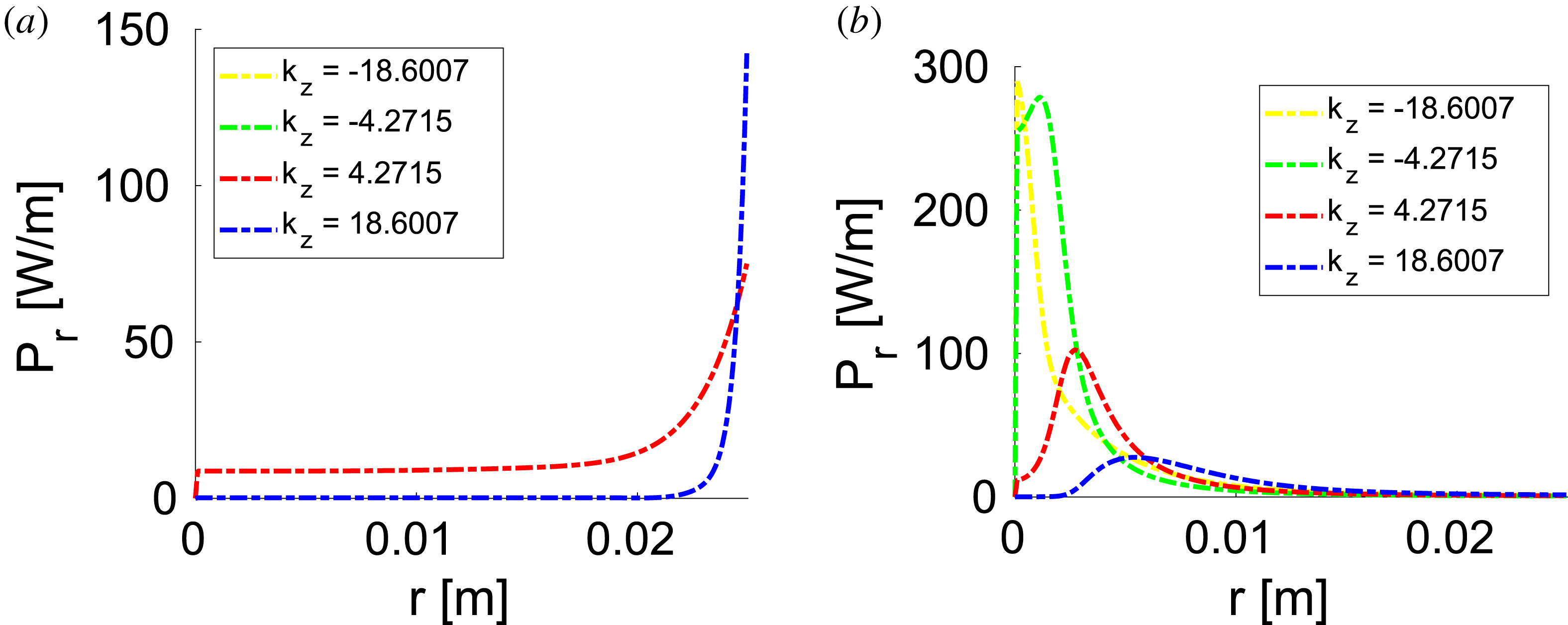
Also in this case, the real part of the power spectrum
 $P_{r}$
is peaked at the outer radius of the source if
 $z=0$
m, and close to the axis if
 $z=0.05$
m (see figure 11). Moreover, the real part of antenna impedance is respectively
 $\text{Re}(Z)=0.2081~\unicode[STIX]{x03A9}$
and
 $\text{Re}(Z)=0.2483~\unicode[STIX]{x03A9}$
for non-uniform and uniform magnetostatic field. In addition, at
 $z=0.05$
m the interval of propagative EM waves is wider near the axis of the source than at the outer radius (see figure 12).
Helmholtz coil configuration for case medium. Real part of the power spectrum (
 $P_{r}$
) as a function of the radial position (
 $r$
), evaluated for different axial wavenumbers (
 $k_{z}$
). (a) Centre of the discharge
 $z=0$
m; (b) boundary of the discharge
 $z=0.05$
m.

Helmholtz coil configuration for case medium: interval of propagative EM waves, expressed in terms of axial wavenumber
 $k_{z}$
, along the radius of the discharge. The propagative interval is included between the minimum propagative
 $k_{z}$
(Min), and the maximum (Max). (a) Centre of the discharge
 $z=0$
m; (b) boundary of the discharge
 $z=0.05$
m.

4.2.3 Case high
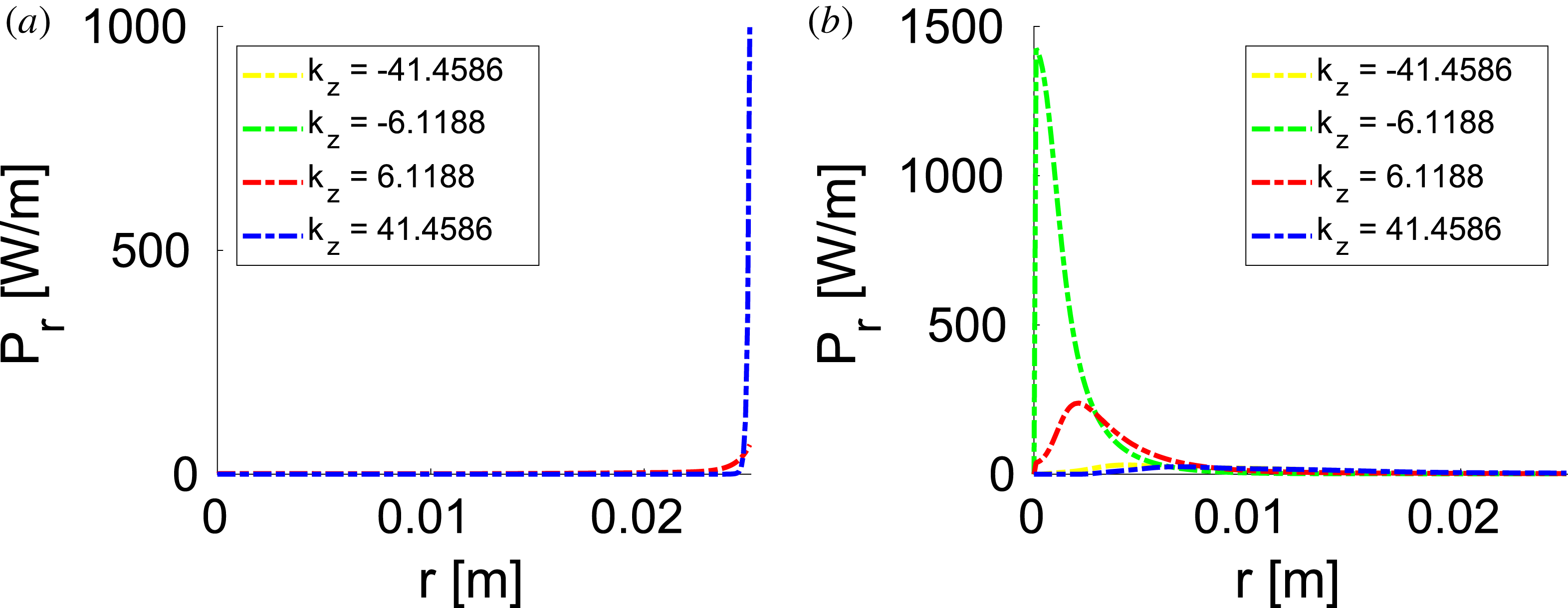
As in case low and case medium, at
 $z=0.05$
m the real part of the power spectrum is peaked near the axis of the source, and at
 $z=0$
m near the outer radius (see figure 13). Moreover, the real part of the antenna impedance is respectively
 $\text{Re}(Z)=0.8496~\unicode[STIX]{x03A9}$
and
 $\text{Re}(Z)=0.9345~\unicode[STIX]{x03A9}$
for non-uniform and uniform magnetostatic fields. Finally, at
 $z=0.05$
m the interval of propagative EM waves is wider near the axis of the source than at the outer radius (see figure 14).
Helmholtz coil configuration for case high. Real part of the power spectrum (
 $P_{r}$
) as a function of the radial position (
 $r$
), evaluated for different axial wavenumbers (
 $k_{z}$
). (a) Centre of the discharge
 $z=0$
m; (b) boundary of the discharge
 $z=0.05$
m.

Helmholtz coil configuration for case high: interval of propagative EM waves, expressed in terms of axial wavenumber
 $k_{z}$
, along the radius of the discharge. The propagative interval is included between the minimum propagative
 $k_{z}$
(Min), and the maximum (Max). (a) Centre of the discharge
 $z=0$
m; (b) boundary of the discharge
 $z=0.05$
m.

5 Three-dimensional analysis
The same problem as that studied in § 4 has been tackled with the ADAMANT code, namely 3-D power deposition profile
 ${\mathcal{E}}_{\text{pow}}$
and antenna impedance
 $Z$
have been calculated. The helicon source at hand has radius
 $R=0.025$
m and length
 $L=0.10$
m. Uniform plasma has been assumed, and two geometries of magnetostatic field, generated respectively by Helmholtz and Maxwell coils (see figure 2), have been studied. As in § 4, we have simulated three configurations, namely case low, case medium and case high. In the following, due to the inherent symmetry of the problem, the 3-D power deposition profile
 ${\mathcal{E}}_{\text{pow}}$
has been reported only on a radial cut of the plasma cylinder. In addition, provided that
 ${\mathcal{E}}_{\text{pow}}$
scales with the square of the voltage imposed at the antenna port
 $V_{G}$
, its value has been reported in arbitrary units (A.U.).
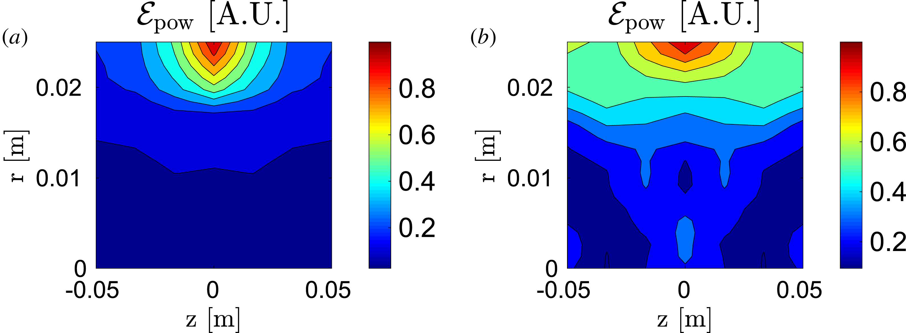
In figure 15, we have depicted the
 ${\mathcal{E}}_{\text{pow}}$
map in the case high. When the magnetostatic field is generated by either Maxwell (see figure 15
a) or Helmholtz (see figure 15
b) coils, the power deposition profile is peaked in correspondence with the outer radius of the plasma discharge. For the Maxwell coil configuration, these results are in agreement with the SPIREs calculations (see § 4.1). Instead, in the Helmholtz coil configuration, SPIREs estimates a centrally peaked power deposition (see § 4.2). The disagreement found between ADAMANT and SPIREs must be attributed to the 1-D radial formulation of the latter. In fact in SPIREs, the effects induced by axial gradients of the magnetostatic field, such as wave reflections (Lafleur et al.
Reference Lafleur, Charles and Boswell2011), cannot be properly simulated. Moreover, the real part of the antenna impedance calculated by ADAMANT is
 $\text{Re}(Z)=0.8372~\unicode[STIX]{x03A9}$
and
 $\text{Re}(Z)=0.8028~\unicode[STIX]{x03A9}$
respectively for the Maxwell and the Helmholtz magnetic geometries; instead, for the uniform field
 $\text{Re}(Z)=0.8375~\unicode[STIX]{x03A9}$
. In the Maxwell (Helmholtz) configuration
 $\text{Re}(Z)$
is comparable with (lower than) the uniform case, as previously predicted by SPIREs, see § 4.2. Finally, it is worth recalling that similar considerations hold true also in the case low and case medium, not reported for the sake of brevity.
Three-dimensional power deposition profile (
 ${\mathcal{E}}_{\text{pow}}$
) as a function of the radial (
 $r$
) and axial (
 $z$
) position;
 ${\mathcal{E}}_{\text{pow}}$
is expressed in A.U: (a) Maxwell coils and (b) Helmholtz coils; case high.

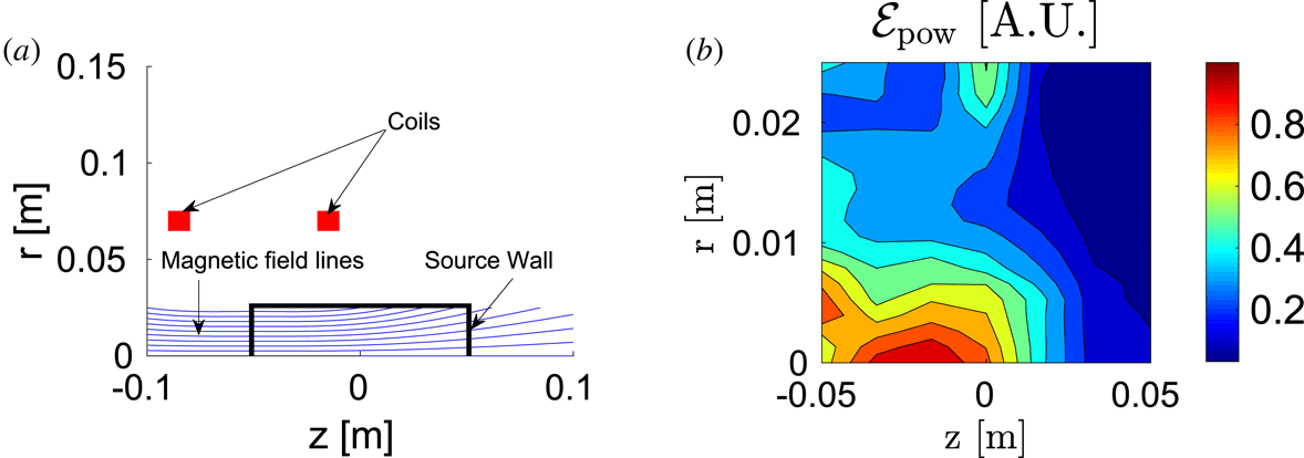
(a) Draft of the magnetic field geometry generated by translated Helmholtz coils. (b) Three-dimensional power deposition profile (
 ${\mathcal{E}}_{\text{pow}}$
) as a function of the radial (
 $r$
) and axial (
 $z$
) position;
 ${\mathcal{E}}_{\text{pow}}$
is expressed in A.U.; case high.

In order to further investigate the reliability of the SPIREs code, we have analysed another magnetic geometry, obtained by translating the Helmholtz coils with respect to the plasma cylinder (see figure 16
a). We have reported the corresponding
 ${\mathcal{E}}_{\text{pow}}$
map in figure 16(b); case high has been considered. Interestingly, the power deposition profile is peaked in correspondence with the axis of the discharge and is not symmetric with respect to
 $z=0$
cm. Such a result is coherent with the SPIREs predictions, in fact the power spectrum reported in figure 13(b) is centrally peaked. Moreover, the absence of symmetry in
 ${\mathcal{E}}_{\text{pow}}$
can be justified by the higher power content associated with negative axial wavenumbers (see figure 13
b). In addition, we report that the real part of the antenna impedance calculated with this last magnetic configuration is
 $\text{Re}(Z)=0.7962~\unicode[STIX]{x03A9}$
, namely lower than for the uniform field (
 $0.8375~\unicode[STIX]{x03A9}$
). Finally, it is worth mentioning that a centrally peaked power deposition profile has been previously predicted by both Kinder & Kushner (Reference Kinder and Kushner2001), Bose et al. (Reference Bose, Govindan and Meyyappan2003) in presence of a non-uniform magnetostatic field.
6 Conclusions
We have studied the power deposition phenomenon in a cylindrical helicon source with both the 1-D radial code SPIREs (Melazzi et al.
Reference Melazzi, Curreli, Manente, Carlsson and Pavarin2012) and the 3-D EM solver ADAMANT (Melazzi & Lancellotti Reference Melazzi and Lancellotti2014). We have analysed two configurations of magnetostatic field, namely that produced by Maxwell coils, and by Helmholtz coils. For each configuration we have studied three cases, namely: (i) low density
 $n=10^{17}~\text{m}^{-3}$
and low magnetic field
 $B_{0}=250$
G; (ii) medium density
 $n=10^{18}~\text{m}^{-3}$
and medium magnetic field
 $B_{0}=500$
G; (iii) high density
 $n=10^{19}~\text{m}^{-3}$
and high magnetic field
 $B_{0}=1000$
G.
In accordance with both solvers, we have found that:
(i) The Maxwell coil configuration does not significantly modify the power deposition with respect to a perfectly uniform and axial magnetostatic field, namely comparable antenna impedances (difference below
 ${<}1$
%) and radially peaked power deposition profile.
(ii) With the Helmholtz coil magnetic geometry the antenna impedance is roughly 10 % lower than with a uniform magnetostatic field.

At the same time, the Helmholtz coil configuration presents: (i) a radially peaked power deposition profile in accordance with ADAMANT, and (ii) a centrally peaked power spectrum in accordance with SPIREs. The discrepancy between the two codes has been resolved by analysing with ADAMANT a magnetic geometry obtained by translating axially the Helmholtz coils with respect to the plasma column. The latter configuration has lead to a centrally peaked and asymmetric power deposition profile.
In the Helmholtz coil configuration, both the impedance reduction and the centrally peaked power deposition profile are associated with a non-uniform interval of propagative EM waves. In fact, analysing the system with the dispersion relation of Cardinali et al. (Reference Cardinali, Melazzi, Manente and Pavarin2014), we have found that the magnetostatic field non-uniformity induces dumping at the outer radius of the discharge of EM waves which are propagative close to the axis.
In conclusion, it is worth recalling that in reality the plasma density in a helicon source is not uniform (Tysk et al. Reference Tysk, Denning, Scharer and Akhtar2004). Nonetheless, in order to keep the analysis lucid, we have investigated the power deposition phenomenon only for a homogeneous plasma. Although the Stix tensor can be a function of the position both in SPIREs and ADAMANT; therefore, the effect of a non-uniform plasma might be the subject of a future work.