1. Introduction
The global climate is changing and even dramatic curbs to greenhouse gas emissions will not prevent it from continuing to do so. The Intergovernmental Panel on Climate Change (IPCC) forecast in its Fourth Assessment Report that, in the absence of emissions abatement, the global average temperature could increase by up to 6.4 °C this century, or moreFootnote 1 (IPCC, Reference Solomon, Qin, Manning, Chen, Marquis, Averyt, Tignor and Miller2007). Of course, significant emissions abatement may well take place. Nevertheless, even if the atmospheric concentration of greenhouse gases were to have been held at its level in the year 2000 (which has not happened), the earth would ‘likely’Footnote 2 still warm by between 0.3 and 0.9 °C this century (IPCC, Reference Solomon, Qin, Manning, Chen, Marquis, Averyt, Tignor and Miller2007). This immediately raises the question of how economies should adapt to changing climatic conditions.
The challenge of adapting to climate change is greatest in developing countries (e.g., Tol et al., Reference Tol, Downing, Kuik and Smith2004; Mendelsohn et al., Reference Mendelsohn, Dinar and Williams2006), for three reasons. The first is geography. Many developing countries are located in tropical and subtropical regions and as such are already hotter than is optimal for various forms of economic activity. Further increases in temperature will lead to conditions that are less favourable still (Mendelsohn and Schlesinger, Reference Mendelsohn and Schlesinger1999). Of course, climate change is about much more than just temperature; many of its impacts are expected to stem from changes in the availability of water. Here too, developing countries are often poorly placed, already experiencing especially low or high average rainfall, and/or high intra- and inter-annual variability (e.g., the Indian monsoon). The second reason is often called sensitivity: a relatively large share of developing countries' output emanates from sectors especially sensitive to climatic conditions, notably agriculture. More broadly, the concept of sensitivity can capture the fact that many people in developing countries are already pursuing marginal livelihoods. The third reason is a lack of adaptive capacity. Developing countries often lack the resources to adapt to climate change, including financial resources (both savings and access to credit), good governance, infrastructure and information.
It is worth being more specific about what adaptation to climate change is. The IPCC has defined it as ‘any adjustment in natural or human systems in response to actual or expected climatic stimuli or their effects, which moderates harm or exploits beneficial opportunities’ (Smit et al., Reference Smit, McCarthy, Canziani, Leary, Dokken and White2001). Within the set of adjustments they refer to, it is often important to further distinguish between ‘flow’ and ‘stock’ adaptation. Flow adaptation includes the set of adjustments for which both the costs and benefits accrue in a single time period, for example, changes in variable agricultural inputs such as crop varieties and fertilizer, and changes in space heating and cooling. By contrast, stock adaptation is a form of investment in which costs are paid up front, while benefits accrue in several future time periods, for example, dykes that protect against coastal flooding, or dams that store water to cope with droughts. But stock adaptation can take other, more indirect forms, such as investing in health care infrastructure in order to cope with a changing burden of disease, or investing in agricultural extension services to support flow adaptations by farmers. In this paper, we focus on adaptation as an investment problem: i.e., in stock adaptation.
This brings us to a second important distinction, which lies at the heart of our paper, between adaptation to climate change and general economic development. Without wishing to oversimplify, one can identify two schools of thought on the best adaptation strategy in the developing world. The first argues that ‘development is the best form of adaptation’: it is better to prioritize traditional developmental goals – i.e., investing in physical and human capital stocks and robust institutions – over defensive investments aimed specifically at reducing vulnerability to climate change. The rationale for this claim may be traced back to Thomas Schelling (Reference Schelling1992), who reasoned that, given developing countries are vulnerable to climate change due in large part to their high sensitivity and low adaptive capacity, both of which are essentially problems of their low level of development, ‘their best defense against climate change may be their own continued development’ (Schelling, Reference Schelling1992: 6). It is important to note that Schelling was thinking about whether adaptation, as opposed to emissions abatement, was the best policy response to climate change. Nevertheless, his suggestion has given rise to subsequent work arguing more directly that development is the best form of adaptation (e.g., Mendelsohn, Reference Mendelsohn, Hahn and Ulph2012; Fankhauser and Burton, Reference Fankhauser and Burton2011). The second school of thought argues that ‘development is contingent on adaptation’: the process of development will be severely compromised by climate change, unless specific adaptation takes place. In this view, successful defensive adaptation is a necessary condition for the effective accumulation of capital stocks and the welfare improvements associated with development. This is most notably the policy position adopted by various international development organizations (e.g., UNDP, 2007; World Bank, 2010).
There is a burgeoning literature on adaptation to climate change, but much of it is based on local case studies. Just a few studies have emerged to consider adaptation as a macro-economic issue. Their primary purpose has been to quantify the costs of adaptation at the national and regional levels, in support of international political negotiations to agree payments for adaptation from industrialized to developing countries. Fankhauser (Reference Fankhauser2010) divides this literature into a ‘first’ and ‘second’ generation. The first-generation studies were very basic indeed. Their approach was simply to estimate the fraction of current investment flows sensitive to climate change, and then to multiply these flows by a mark-up coefficient representing an aggregate estimate of how much it would cost to ‘climate-proof’ them (World Bank, 2006a; Stern, Reference Stern2007; UNDP, 2007). This approach was static, and the mark-up coefficient in particular had almost no empirical basis. The second generation of studies commenced with UNFCCC (2007), which delved into the detail of adaptation costs across the main climate-sensitive sectors. It thus enjoyed a sounder empirical basis, but remained static. A recent World Bank (2010) study quantified adaptation costs over time, but was critically limited by the assumption that adaptation is undertaken up to the point at which all climate damage is eliminated – this cannot be efficient. Indeed, this is the main criticism levelled at all of these studies by proponents of the view that development is the best form of adaptation: i.e., that no, or insufficient, attention is paid to the benefits of adaptation, whether those benefits exceed the costs, and whether alternative uses of scarce resources to invest in productive capital would yield greater net benefits (Mendelsohn, Reference Mendelsohn, Hahn and Ulph2012).
A few recent studies have extended ‘integrated assessment models’ (IAMs) of the coupled climate–economy system to include adaptation as a control variable. Previously, IAMs either paid no attention to adaptation, or else it was implicit in the function determining climate damages, and thus could not be varied by the planner. Adaptation-IAMs include a dynamic representation of adaptation, and quantify its benefits. They have confirmed that optimal adaptation leaves some ‘residual’ damages from climate change, and that optimal climate policy involves both adaptation and emissions abatement. In addition, they embody a great deal of careful calibration work, which others, like us, can make use of. However, at present the conclusions one can draw from this literature for thinking about the links between adaptation and development are limited. First, the literature has various limitations of scope: some models are, for example, confined to a global aggregation (AD-DICE in Agrawala et al., Reference Agrawala, Bosello, Carraro, de Bruin, De Cian, Dellink and Lanzi2010), or only consider flow adaptation (de Bruin et al., Reference de Bruin, Dellink and Tol2009). Secondly, the literature is confined to numerical simulation, so it has yet to advance a formal understanding of the analytical foundations of the problem. Thirdly, the numerical simulations have been highly complex, especially in the largest models (AD-RICE and AD-WITCH in Agrawala et al., Reference Agrawala, Bosello, Carraro, de Bruin, De Cian, Dellink and Lanzi2010), and consequently they have been largely reliant on a single-model parameterization. This is a significant shortcoming, because the estimation of the costs and benefits of adaptation, particularly at the level of nations and regions, is well known to be highly uncertain (Agrawala and Fankhauser, Reference Agrawala and Fankhauser2008).
The aim of this paper is to formalize and improve our understanding of the relationship between adaptation and growth/development in developing countries, using neoclassical growth theory. What is the optimal balance between investment in traditional productive capital (i.e., ‘development’) and diverting resources into adapting to climate change? Perhaps more importantly, given the uncertainties, how robust is this balance to changes in the values of key parameters? In section 2, we present a tractable analytical model of optimal growth and adaptation. Investments can be made either in productive capital that is vulnerable to climate change, or in adaptive capital, which is not inherently productive, but reduces climate damages. We derive expressions for the optimal controls and show that, even in a highly simplified model, the task of apportioning investment between the two capital stocks is subtle. We can virtually rule out the possibility that the optimal investment strategy invests nothing in adaptive capital but, beyond that, answers to questions about the dependence of investment in adaptive capital on the level of development – as measured by the stock of vulnerable capital – and about just how much should be invested depend on empirical circumstances. Therefore we make an empirical application of our model to sub-Saharan Africa (section 3), which is widely regarded to be the region of the world that is most vulnerable to climate change. We show that, in our base-case calibration, the optimal strategy requires the stock of adaptive capital to grow significantly faster than the stock of vulnerable capital. Nevertheless, the optimal adaptive sector represents less than 1 per cent of the economy over the next 100 years in the optimal solution. Importantly, we show that this finding is robust to changes in the values of a wide range of key parameters. The two exceptions are an adaptation effectiveness parameter and the initial stock of adaptive capital, both of which can change the qualitative features of the optimal trajectory. Section 4 discusses these results and possible extensions, and concludes.
2. A model of economic growth with investment in adaptation
Our model builds on the standard Ramsey–Cass–Koopmans growth model, which has formed the basis of much related work in climate change economics (e.g., Nordhaus, Reference Nordhaus2008). The model is designed with regions with small shares of global CO2 emissions in mind, so that the magnitude of realized climate change may be treated as exogenous to the region's development choices. This is a mild assumption for all developing countries with the exception of China, which currently accounts for approximately 22 percent of global CO2 emissions. The next largest emitter in the developing world, India, accounts for only 5 per cent of global emissions.
The economy in our model consists of two capital stocks – vulnerable capital K V , which is productive but susceptible to climate impacts, and adaptive capital K A , which is not inherently productive but reduces the impacts of climate change on the output from vulnerable capital. In order to interpret the model correctly, it is crucial to realize that any given investment project could contribute to the stocks of both K A and K V . Consider as an example the construction of a dam 10 ms high. Suppose that there is limited water availability in the supply region of the dam, so that it increases production even in today's climate. If, say, the optimal height of the dam in today's climate is 8 m, the first 8 m of dam will contribute to the stock of K V . Suppose, however, that under climate change water stress increases relative to today, requiring a larger dam for optimal production. Then the last 2 m of the dam will contribute to the stock of K A – this part of the dam is unproductive in the absence of climate change, and its productivity increases as temperatures (a proxy for water availability) rise. Thus K A aggregates all the protective stocks in the economy that are additional to the optimal protection level for the current climate. Clearly, many developing countries are insufficiently protected against current climate variability. However, investments which reduce vulnerability to current climate are rightly classified as ‘development’, not adaptation to climate change.
In our model, vulnerable capital K V combines with an exogenous labour time series L(t) to produce output A(t)F(K V ,L), where A(t) is an exogenous total factor productivity time series, and F is the production function. The following conditions on the production function F, as well as the Inada conditions, are assumed to hold (subscripts denote partial derivatives):
 $$F_{K_{V}} \gt 0\comma \; F_{K_{V}K_{V}} \lt 0\comma \; F_{L} \gt 0\comma \; F_{LL} \lt 0$$
 $$F\lpar mK_{V}\comma \; mL\rpar =mF\lpar K_{V}\comma \; L\rpar .$$
Thus there are diminishing returns to each of the factors of production, and the production technology exhibits constant returns to scale.
In keeping with much of the literature on modelling climate damages, gross output in our model is modified by a multiplicative damage function, which is a function of global temperature change X. Unlike models which focus on mitigation, however, damages in our model may be ameliorated by accumulating a stock of adaptive capital K A . We model the interaction between the level of climate change and the stock of adaptation through the modified damage multiplier D(K A , X), which represents damages net of adaptation. The damage multiplier D(K A , X) is assumed to satisfy
 $$ D \colon {\open R}^{+} \times {\open R}^ {+} \rightarrow\lsqb 0\comma \; 1\rsqb $$
 $$ \forall K_{A}\comma \; D\lpar K_{A}\comma \; 0\rpar =1\comma \; \, \, D_{a}\lpar 0\comma \; X\rpar \ge 0 \, \, for\, \, X \gt 0 $$
 $$D_{a} \ge 0\comma \; \, \, D_{aa} \le 0\comma \; \, \, D_{aX} \gt 0\comma \; \, \, D_{X} \lt 0 $$
where
 $D_{a}=\displaystyle{{\partial D} \over {\partial K_{A}}}$
,
 $D_{aa}=\displaystyle{{\partial^{2}D} \over {\partial K_{A}^{2}}}$
,
 $D_{X}=\displaystyle{{\partial D} \over {\partial X}}$
,
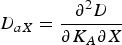 $D_{aX}=\displaystyle{{\partial^{2}D} \over {\partial K_{A}\partial X}}$
. Damages thus reduce gross output by a factor D, which decreases with the magnitude of climate change X (i.e., D
X
< 0). D is defined so that adaptation has no benefit when there is no climate change (i.e., D(K
A
, 0) = 1). In addition, the marginal unit of adaptation is always beneficial (D
a
≥ 0 for X > 0), but exhibits decreasing returns (D
aa
≤ 0). Finally, the condition D
aX
> 0 implies that an additional unit of adaptive capital is more effective at reducing damages when temperature change is large than when it is small.
The evolution of the two capital stocks is given by
 $$\dot{K}_{V} =A\lpar t\rpar D\lpar K_{A}\comma \; X\lpar t\rpar \rpar F\lpar K_{V}\comma \; L\lpar t\rpar \rpar -\delta_{V}K_{V}-cL\lpar t\rpar -Q\lpar I\rpar $$
 $$\dot{K}_{A} =I-\delta_{A}K_{A} $$
where c is consumption per capita, I is investment in adaptive capital, and Q(I) is the cost of investment in adaptive capital of magnitude I, which satisfies Q
′(I) >0, Q
′′(I) ≥ 0. The convexity of Q acts as a reduced form ‘brake’ on the pace of adaptation, as large investment flows are penalized more heavily than small ones (Eisner and Strotz, Reference Eisner and Strotz1963; Lucas, Reference Lucas1967). To see the impact of a convex Q(I), consider a scenario where temperature change does not occur until, say, t = 50 years (X(t) = 0 for t < 50), after which it jumps to some constant value
 $\bar{X}$
. In this case, if Q = I, the planner is indifferent between making a series of small investments and making one large investment of equal magnitude. Since the marginal benefit of adaptive investment is zero for the first 50 years, the planner's positive discount rate will cause her to invest only very small amounts in the early periods, and to defer the bulk of adaptive investment until t ≈ 50, when its payoffs will be more immediate. When Q is convex, however, the planner has an incentive to build up adaptive capital stocks gradually over the first 50 years – a lot of small annual investments will be less costly than a large and rapid one-off investment as t approaches 50 years. Thus the convexity of Q is a measure of the incentive the planner has to make cumulative, anticipatory plans, rather than waiting and making one big adaptive push. Investments in stock adaptation may incur convex costs since, unlike investments in the vulnerable sector (most of which will be private decisions), they will be largely publicly funded (Stern, Reference Stern2007), and are thus subject to planning costs, policy delays due to the political process, liquidity constraints and perhaps even corruption.Footnote
3
Finally, the parameters δ
V
and δ
A
are the depreciation rates of vulnerable and adaptive capital, respectively.
The social planner chooses the values of c and I so as to maximize the following classical utilitarian objective function:
 $$W= \int_{0}^{T}L\lpar t\rpar U\lpar c\rpar e^{-\rho t}dt\comma \; $$
subject to the constraints (6–7). Under the assumptions specified above, the control problem is convex, and thus has a unique solution, with the Pontryagin conditions being necessary and sufficient for an optimum. In our simulation work we will take the time horizon T to be large (T = 500 years), and following Nordhaus and Boyer (Reference Nordhaus and Boyer2000), impose terminal conditions on the state variables such that K V (T) = K A (T) = 0. Then, with a moderate discount rate ρ, policy choices for the first several hundred years are relatively insensitive to the terminal conditions. Note that we are uninterested in the properties of any putative steady state, as the relevant policy issues concern transient adaptation to a dynamically evolving climate.
Applying the Pontryagin conditions to this control problem, the Euler equations for the optimal controls are:
 $$ \dot{c} =\displaystyle{{c} \over {\eta\lpar c\rpar }} \left[A\lpar t\rpar D\lpar K_{A}\comma \; X\lpar t\rpar \rpar F_{K_{V}}-\delta_{V}-\rho\right]\semicolon \; $$
 $$\eqalign{\dot{I} & = \displaystyle{{Q^{\prime}\lpar I\rpar } \over {Q^{\prime\prime}\lpar I\rpar }} \left[A\lpar t\rpar D\lpar K_{A}\comma \; X\lpar t\rpar \rpar F_{K_{V}}-\delta_{V}+\delta_{A}\right]\cr & \quad -\displaystyle{{1} \over {Q^{\prime\prime}\lpar I\rpar }} A\lpar t\rpar D_{a}\lpar K_{A}\comma \; X\lpar t\rpar \rpar F\lpar K_{V}\comma \; L\lpar t\rpar \rpar }$$
where
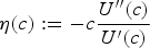 $\eta\lpar c\rpar :=-c \displaystyle{{U^{\prime\prime}\lpar c\rpar } \over {U^{\prime}\lpar c\rpar }}$
is the elasticity of marginal utility. In general, a solution to this problem requires us to specify initial and terminal values for the stocks K
V
and K
A
, and integrate the four-dimensional dynamical system comprising the state equations (6–7) and Euler equations (9–10). The initial values of the controls are determined endogenously by the requirement that the solution satisfy the terminal conditions. This is a complex procedure, and since the model is a nonlinear coupled dynamical system, it is difficult to say anything in general about the dependence of the adaptive investment rule on the state variables.Footnote
4
Despite the complexity of even this simple model, it is desirable to have an analytical handle on the dependencies of the investment rule. To this end, we consider the limit in which the adjustment cost function approaches the linear function Q(I) = I, i.e., Q ′(I) = 1, Q ′′(I) = 0. In this limit the optimal control problem becomes singular, and without imposing constraints on the controls, the solution will instantly adjust the capital stocks so that the algebraic relation
 $$A\lpar t\rpar D\lpar K_{A}\comma \; X\lpar t\rpar \rpar F_{K_{V}}-A\lpar t\rpar D_{a}\lpar K_{A}\comma \; X\lpar t\rpar \rpar F\lpar K_{V}\comma \; L\lpar t\rpar \rpar = \delta_{V}-\delta_{A} $$
is satisfied at each point in time. That is, the optimal singular control sets the difference between the marginal productivities of vulnerable and adaptive capital stocks equal to the difference between their depreciation rates. This is a familiar result from two-sector growth models (see, e.g., Acemoglu, Reference Acemoglu2008: 369). The difference here is the additional exogenous time-series X(t), which moderates the productivity of the economy and affects the dynamics of investment allocations. Defining the intensive variable k V = K V /L(t) and f(k V ): = F(k V ,1), and differentiating (11) with respect to time, one can show that optimal investment in adaptive capital is given by
 $$I=R_{X}\dot{X}+R_{V}\dot{k}_{V}+R_{H}\dot{H}+\delta_{A}K_{A}\comma \; $$
where
 $$H\lpar t\rpar := \displaystyle{{\delta_{V}-\delta_{A}} \over {A\lpar t\rpar L\lpar t\rpar }}\comma \; $$
and where we define the ‘response rates’ R X , R V and R H , which determine the adaptive investment response to changes in the values of X, k V and H, respectively, through
 $$R_{X} :=\displaystyle{{D_{aX}-\displaystyle{{f^{\prime}} \over {f}}D_{X}} \over {\displaystyle{{f^{\prime}} \over {f}} D_{a}-D_{aa}}} $$
 $$R_{V} :=\displaystyle{{D_{a}- \displaystyle{{f^{\prime\prime}} \over {f^{\prime}}}D} \over {D_{a}-\displaystyle{{f} \over {f^{\prime}}}D_{aa}}}.$$
 $$R_{H} := \displaystyle{{1} \over {D_{a}f^{\prime}-D_{aa}f}}.$$
The first term in (12) is the most interesting, as it represents the direct effect of the climate dynamics on the investment rule. The second term is an adjustment term which represents an income effect on the optimal combination of adaptive and vulnerable capital. It would be present even if the climate were not changing (i.e.,
 $\dot{X}=0$
), but the economy were growing (or declining), as resources would need to be moved between sectors so that (11) is satisfied. The third term in (12) arises from the exogenously evolving time series A(t) and L(t) in the model, and is also an ‘exogenous adjustment’ term. Note that this term falls away if the depreciation rates of adaptive and vulnerable capital are equal (i.e., δ
V
= δ
A
), and in general is likely to be negligibly small owing to the large values of A(t) and L(t) in empirical applications. Finally, the fourth term is simply the investment needed to ensure that adaptive capital does not depreciate.
To begin analyzing this expression, notice that:
Remark 1
If
 $\dot{X}>0$
,
 $\dot{k}_{V}>0$
, and
 $\delta_{V}\leq\delta_{A}$
then
 $I>\delta_{A}K_{A}$
.
Proof: The definitions (14–16) and the assumptions (5) imply that R X > 0, R V > 0, and R H > 0. The result follows immediately, assuming that A(t)L(t) is increasing in t. □
In addition, we have:
Proposition 1
The response rates R X , R V , R H depend on k V as follows:
-
1. R X is an increasing (decreasing) function of k V when ε a,a < (>)ε X,a , where ε a,a is the elasticity of D a with respect to K A , and ε X,a is the elasticity of D X with respect to K A .
-
2. R V is a decreasing function of k V .
-
3. R H is an increasing (decreasing) function of k V when f ′′/f ′ < (>)D aa /D a .
Proof: See appendix A.Footnote 5 □
Remark 1 implies that if we are in a regime in which temperatures are rising, and the economy is developing simultaneously, it is very likely optimal to increase the stock of adaptive capital above its ‘replacement’ level (the term δ
A
K
A
is just the depreciation in the adaptive capital stock). We say only ‘very likely’, since the proposition requires δ
V
≤ δ
A
, which is not guaranteed empirically. However, this condition arises from the requirement that
 $\dot{H}>0$
. As noted above, this term is small in comparison to the other three terms in (12), so its contribution is likely negligible. This remark thus argues against the strongest version of the ‘adapt through development’ hypothesis, which requires adaptive investments to be identically zero. Positive investment in adaptation (albeit of unknown magnitude at this point) is very likely optimal, even when the economy is accumulating traditional vulnerable capital as well.
Proposition 1 allows us to compare the adaptive investment plans of more and less developed economies, in particular demonstrating how the investment rule changes as the stock of per capita vulnerable capital increases. Assume once again that the
 $\dot{H}$
term is negligible. Then, all else being equal, more developed economies will respond proportionately less to a change in the capital stock
 $\dot{K}_{V}$
than their less developed counterparts, since
 $\displaystyle{{\partial R_{V}} \over {\partial K_{V}}}<0$
. However, it is possible that this reduction in the response rate R
V
may be offset by an increase in investment due to the change in X. In order for this to be possible, we require ε
a,a
< ε
X,a
. This condition on the elasticities of the damage function says that, in order for wealthier economies to respond proportionately more to climate change
 $\dot{X}$
, the damage reduction effect of the marginal unit of adaptive capital should outweigh its effect on the returns to adaptive investment, which are decreasing in the stock of adaptive capital. Note that the condition depends both on the structure of the damage function D(K
A
, X), as well as on the values of K
A
, X. It may be satisfied at some points in time over a country's development trajectory and not at others, as the magnitude of climate change X changes and the capital stock K
A
evolves. Since in general we do not know that ε
a,a
> ε
X,a
for all values of X, K
A
a priori, we cannot conclude that a wealthier economy has less need for adaptation.
Taken together, these results suggest that, even in this highly simplified model, the task of apportioning investment between productive and adaptive capital is a subtle one, and certainly not reducible to simplistic prescriptions. While Remark 1 gives us an indication of the sign of adaptive investment over an economy's development pathway, and Proposition 1 allows us to determine how the investment rule is affected by different stocks of vulnerable capital, they cannot give us quantitative information about the optimal levels of adaptive and vulnerable capital stocks for a given country over time. In order to investigate this, we now turn to full numerical solutions of the model, and investigate their sensitivity to underlying assumptions about the economy, the effectiveness of adaptation and the magnitude of climate change.
3. Application to sub-Saharan Africa
The analytical results discussed above are limited, in that they do not account for the effect of adjustment costs on the investment rule, or tell us about the level and trajectory of adaptive investment, relative to investment in vulnerable capital. In order to address these questions one must compute the optimal controls explicitly. To this end, we now calibrate our model to a specific region – sub-Saharan Africa. There are two good reasons for focussing our attention on this region. First, it makes a small contribution to global greenhouse gas emissions (less than 5 per cent of total CO2-equivalent emissions; EarthTrends, 2009), and its share in emissions is unlikely to grow substantially over the coming decades. Thus our assumption that climate change is exogenous holds to a good approximation. Secondly, and more importantly, the region is highly vulnerable to climate impacts (Boko et al., Reference Boko, Parry, Canziani, Palutikof, van der Linden and Hanson2007), and thus has a strong incentive to understand how best to protect itself against their effects.
3.1. Model calibration and implementation
To calibrate and simulate the model, it is necessary to make choices for the functions D(K A , X), F(K V , L), Q(I) and U(c). We take
 $$D\lpar K_{A}\comma \; X\rpar =\displaystyle{{1+g\lpar K_{A}\rpar } \over {1+g\lpar K_{A}\rpar +f\lpar X\rpar }}\comma \; $$
where
 $$f\lpar X\rpar = \alpha_{1}X+\alpha_{2}X^{2} $$
 $$g\lpar K_{A}\rpar = \beta_{1}K_{A}^{\beta_{2}}.$$
β1 > 0, β2 ∈ [0,1] ensures that all the derivatives of D have the correct signs. It is important to note that this choice of damage multiplier implies that D a (0,X) = ∞, so that solutions to the control problem will of necessity be interior. This is in contrast to our analytic results in section 2, in which no assumption was made about the marginal productivity of adaptive capital at zero, other than that it is non-negative. We examine the sensitivity of our results to assumptions about the initial productivity of adaptive capital by performing a sensitivity analysis over the initial value of adaptive capital in section 3.3.3 below.
The quadratic dependence of gross damages on temperature change is commonly assumed in the literature, being in agreement with, for example, Nordhaus and Boyer (Reference Nordhaus and Boyer2000) and Nordhaus (Reference Nordhaus2008) (but see section 4). We pick the Cobb–Douglas form F(K V ,L) = K V γ L 1−γ for γ ∈ [0, 1], and choose
 $$Q\lpar I\rpar =I + \displaystyle{{q} \over {2}}I^{2}\comma \; $$
where q is a parameter which fixes the cost of adjustment from vulnerable to adaptive capital. Finally, our social planner's utility function is assumed to be of the constant relative risk aversion (CRRA) form:
 $$U\lpar c\rpar =\displaystyle{{c^{1-\eta}} \over {1-\eta}} $$
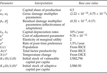
where η > 0 is the elasticity of marginal utility, which parameterizes the planner's desire to smooth consumption over time. A complete specification of the model therefore needs to specify numerical values for the parameters and time series in table 1.
Model parameters and exogenous time series

Notes: Sensitivity analysis is conducted over starred parameters.
Data from Agrawala et al.'s (Reference Agrawala, Bosello, Carraro, de Bruin, De Cian, Dellink and Lanzi2010) comparison of multiple adaptation-IAMs determine values for the gross damage function D(0, X) and residual damages (i.e., damages as a percentage of GDP, as a function of the adaptive capital stock and temperature change). We performed a nonlinear least-squares fit to these data to determine the values of α1 and α2. The parameters β1 and β2 were determined so that D(K A , X) agrees with the calibration values at (K A ,X) = (US$1.1 × 1011,1.25°C) and (K A ,X) = (US$9.7 × 1011,2.25°C). Note that the reduction in damages from flow adaptation is included directly in the calibration of D(0, X),Footnote 6 so while flow adaptation is not a control variable in our analysis, its effects are taken into account. Also implicit in our calibration of damages is the relationship between climate impacts and GDP (excluding the effect of flow and stock adaptation), because the underlying IAM studies on which we calibrate control for it. This is clearly critical for the purposes of the present paper, if we are to assess the relative contributions of investments in productive and adaptive capital in optimally reducing climate vulnerability. One example of how this relationship plays out is in agriculture, where the income elasticity of climate damages (as a percentage of GDP) is thought to be negative, for the simple reason that, as GDP per capita rises, the share of agricultural output in GDP per capita falls. However, different income elasticities exist for different sectors (Nordhaus and Boyer, Reference Nordhaus and Boyer2000; Anthoff and Tol, Reference Anthoff, Tol, Hahn and Ulph2012), and the overall income elasticity of damages is the output-weighted sum across sectors.
The base value of q was calibrated so that 90 per cent of a US$ 30 per capita per year investment in adaptive capital is realized at t = 0. The initial stock of vulnerable capital K V (0), as well as the depreciation rate on K V , was chosen in agreement with the values in the most recent version of the RICE model (discussed in Nordhaus, Reference Nordhaus2010), as was the time series of population L(t).Footnote 7 The depreciation rate on K A was taken from Agrawala et al. (Reference Agrawala, Bosello, Carraro, de Bruin, De Cian, Dellink and Lanzi2010). We set the initial stock of adaptive capital to a nominal US$ 0.50/capita, as current adaptive capital stocks specifically designed to combat the impacts of climate change (as opposed to current climate variability) are negligible in sub-Saharan Africa (see discussion in section 3.3.3). The base case values of the preference parameters ρ and η are in line with much of the literature, although there is a well-known debate about them (Stern, Reference Stern2007; Nordhaus, Reference Nordhaus2008), and we explore the implications of alternative settings in our sensitivity analysis.
As we wished to do sensitivity analysis over the two remaining exogenous time series X(t) and A(t), they were treated slightly differently. The DICE model (Nordhaus, Reference Nordhaus2008) was used to generate temperature trajectories X(t) under three scenarios for the global atmospheric stock of CO2 – business as usual (BAU scenario), stabilization of the atmospheric stock of CO2 at twice its preindustrial level (2CO2 scenario), and stabilization of atmospheric CO2 at 1.5 times the preindustrial level (1.5CO2 scenario). For each of these scenarios, we obtained temperature trajectories for four different values of the climate sensitivity parameter S. Climate sensitivity measures the equilibrium surface warming that results from a doubling of CO2 concentrations – it thus quantifies the magnitude of the temperature response to the increase in radiative forcing that arises from increased concentrations of atmospheric CO2. The value of S is uncertain, due to uncertainties in the instrumental record of temperature changes, and uncertainties about key climatic feedback processes (see Knutti and Hegerl, Reference Knutti and Hegerl2008 for a review of climate sensitivity concepts and estimates). We chose S ∈[1.5°C,3°C,4.5°C,6°C], which approximates the likely range for its values as determined by the scientific literature. We thus obtained 12 unique temperature trajectories, which were used in our sensitivity analysis. These trajectories are plotted in figure A1 in Appendix B. It can readily be seen that both the atmospheric stock of CO2 and the climate sensitivity have a significant effect on the trajectory of X, and consequently we explore a wide range of values.
The series for A(t) in RICE may be fitted exactly by a function of the form
 $$A\lpar t\rpar =A\lpar 0\rpar \exp\left[g_{\infty}t+\displaystyle{{g_{0}-g_{\infty}} \over {\lambda}}\lpar 1-e^{-\lambda t}\rpar \right]\comma \; $$
where initial growth in TFP is g 0 = 2.83 per cent/year, the long-run growth in TFP is g ∞ = 0.23 per cent/year, and the rate of adjustment in the TFP growth rate is λ = 0.01/year for sub-Saharan Africa. Following Nordhaus (Reference Nordhaus2008), we conduct sensitivity analysis over the initial TFP growth rate g 0. The resulting trajectories for A(t) are illustrated in figure A2 in appendix B. Observe that the effect of changes in g 0 on A(t) increases over time.
The model was implemented in MATLAB, and the open-source package GPOPS (Rao et al., Reference Rao, Benson, Darby, Patterson, Franbcolin, Sanders and Huntington2010) was used to find numerical solutions to the optimal control problem. GPOPS uses a generalized colocation method coupled with a high-performance nonlinear optimization routine. This has the advantage of constraining the search for optimal controls to the subset of functions that satisfy the initial and terminal conditions of the problem. This is particularly useful when the optimum is a saddle path equilibrium (as in our case in the T → ∞ limit), as the boundary conditions are automatically satisfied, and the numerical method is more stable than alternatives such as forward- or reverse-shooting (Judd, Reference Judd1998; Atolia and Buffie, Reference Atolia and Buffie2009).
3.2. Base case model results
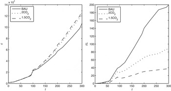
In the first instance, we obtained numerical solutions of the model for our base case calibration, in which climate sensitivity S = 3 °C, and the model parameters are given by the values in table 1. Figure 1 plots the optimal controls, per capita consumption c and per capita investment in adaptation I/L, as a function of time.
Optimal controls for base case model calibration (S = 3 °C)

From the left panel of the figure it is clear that climate change has a significant effect on welfare, even admitting the possibility of adaptation, with the consumption path under BAU significantly below that in the 1.5CO2 and 2CO2 scenarios. The right panel demonstrates, unsurprisingly, that the greater the magnitude of climate change, the greater the level of investment in adaptive capital. Although adaptive investment flows are small relative to consumption, they are not insignificant.
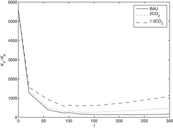
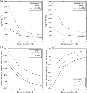
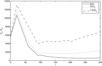
Figure 2 is a core finding of our analysis. It plots the ratio of vulnerable to adaptive capital stocks over time, demonstrating that adaptive capital optimally accumulates at a significantly higher growth rate than vulnerable capital under all three climate change scenarios, at least over the first 100 years. Over the first 50 years, the adaptive sector grows approximately 3.5–5.5 per cent/year faster than the vulnerable sector (see figure 5b). It is important to be clear, however, that there is still over 100 times more vulnerable capital than adaptive capital over the entire model horizon, even under the BAU scenario. This is as it should be, since adaptive capital is not productive. To aid the interpretation of this figure, note that
Ratio of vulnerable to adaptive capital stocks, base case

 $$\displaystyle{{d} \over {dt}} \left(\displaystyle{{K_{V}} \over {K_{A}}}\right)=\left(\displaystyle{{K_{V}} \over {K_{A}}}\right)\lpar g_{V}-g_{A}\rpar \comma \; $$
where g V , g A are the growth rates of vulnerable and adaptive capital, respectively. Thus, when the capital ratio curve is downward sloping, the growth rate of adaptive capital exceeds that of vulnerable capital – this is clearly the case in the first 50 years of the model run. One final qualitative feature of the figure is worth noting – for the first 25 years, the capital ratio curves for the three mitigation scenarios are very close together. This suggests that it is the initial conditions, and not anticipated future climate damages, that dominate the investment rule at early times. The reason for this is that the initial stock of adaptive capital is very low, so that even with climate change of small magnitude at early times, the marginal productivity of adaptive capital is higher than that in the vulnerable sector (due to decreasing returns), leading to rapid growth in the adaptive capital stock. As we shall see in the following section, this result is robust across a large region of the model's parameter space. We perform sensitivity analysis over the initial value of K A in section 3.3.3.
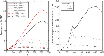
Finally, figure 3 demonstrates the benefits and costs of adaptation. The left panel demonstrates the reduction in damages obtained by the optimal investment policy in each of the three mitigation scenarios. The benefits are significant, especially so in the BAU scenario. The right panel indicates the costs associated with the adaptive investment policy – these are a small fraction of GDP but, through the accumulation of the adaptive capital stock, give rise to a significant amelioration of climate impacts. Thus, in our base case model run, we find that adaptation is an integral part of an optimal development pathway.
Left panel: reduction in damages due to optimal accumulation of adaptive capital; right panel: flow costs of adaptive investment, as %GDP

3.3. Sensitivity analysis
The analysis of the base case model calibration is suggestive, but should certainly not be read as a definitive finding. Many of the parameters used to generate the results are not at all well pinned down in the existing literature (see, e.g., Agrawala and Fankhauser, Reference Agrawala and Fankhauser2008), thus requiring caution when interpreting the results. In this section we submit our results to a sensitivity analysis, in order to investigate their robustness, and understand the effect of alternative choices for parameters on the model solution. We stress that these results examine only the effect of parametric uncertainty in the model, and not the effect of perturbations to the model structure – we discuss the latter in the conclusions.
To begin, it will be useful to define several summary measures that capture useful information about the effect of a change in parameters on the optimal development policy. We define the (Weitzman, Reference Weitzman1976) of a given policy as the value of consumption of consumption per capita which, if held constant, would be equivalent to the welfare achieved by the policy. Formally, if the policy achieves welfare V, the stationary equivalent c* of the policy is defined implicitly through
 $$ \int_{0}^{T}L\lpar t\rpar U\lpar c^{*}\rpar e^{-\rho t}dt=V.$$
Thus the stationary equivalent is a welfare measure denominated in the units of consumption per capita, and is evaluated over the same temporal range as V itself. We will find this useful as a measure of the sensitivity of welfare to model parameters.
Our second set of measures is designed to capture some aspects of the trajectories of the vulnerable and adaptive capital stocks. Clearly, we would like to understand how these trajectories are affected by choices of the model parameters; however, it is unilluminating to plot the full set of trajectories over parameter space. Rather, we focus on descriptive statistics of these time series, which aim to summarize the relative importance of adaptive and vulnerable capital over the development pathway. Our measures are the ratio of vulnerable to adaptive capital after 50 and 100 years, respectively, and similarly, the difference between the average growth rates of vulnerable and adaptive capital over the first two 50-year periods in the model run. The former measure provides static information about the accumulation of each type of capital, while the later supplies dynamic information about their relative rates of change as the economy evolves. The sensitivities of these scalar measures to model parameters are easily represented in two dimensions.
3.3.1. Climate sensitivity and CO2 mitigation scenario
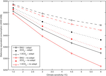
Our first sensitivity analysis examines the effect of different assumptions about the value of climate sensitivity and the CO2 stabilization pathway on welfare in two cases: first assuming optimal investment in vulnerable and adaptive capital, and secondly assuming no adaptation to climate change. The results are summarized in figure 4.
Dependence of welfare on climate sensitivity and global CO2 mitigation scenario, with and without adaptation

The figure shows two important things. First, adaptation is significantly welfare enhancing, especially so in the more extreme climate change scenarios, i.e., low mitigation levels and high climate sensitivity. If one concentrates on the welfare values at the three highest values of S, optimal adaptation is approximately welfare equivalent to a reduction of S by 1.5°C. For example, welfare with optimal adaptation at S = 6°C is approximately equal to welfare without adaptation at S = 4.5°C, in each of the three mitigation scenarios. This approximation does not hold at S = 1.5°C, since welfare has a steep fall-off at low values of S. Secondly, while adaptation is clearly effective, welfare is still strongly sensitive to the magnitude of climate change. Even with optimal adaptation, global mitigation choices are heavily involved in determining domestic welfare. This argues against the sanguine position adopted by some commentators, who suggest that the impacts of climate change may be simply adapted away (Lomborg, Reference Lomborg2007). The figure shows that the difference in welfare between the 1.5CO2 and BAU scenarios is larger than the effect of adaptation in either of them. Welfare may be significantly improved by adopting a more ambitious mitigation policy, especially in a high climate sensitivity world.
Figures 5a and 5b demonstrate that our finding that adaptive capital should grow more rapidly than vulnerable capital over the first 100 model years is robust across the range of mitigation scenarios and climate sensitivity values in figure A1, appendix B. The ratio of vulnerable to adaptive capital is decreasing in S (figure 5a), since higher S implies greater climate damages, and thus a greater need for adaptive capital. Figure 5b shows that adaptive capital grows substantially faster than vulnerable capital for the first 50 years, with the absolute difference in their growth rates increasing as a function of S. Interestingly, this relationship is inverted over the second 50 model years – although adaptive capital still grows faster than vulnerable capital over this period, the absolute difference in growth rates is smaller the larger is S. Larger S means a greater need for adaptation, and thus a more rapid initial investment in adaptive capital. However, since the stock of adaptive capital is larger for high S, the effects of decreasing returns are felt more for larger S as well. This makes vulnerable capital more competitive after the initial spurt of adaptive capital accumulation, and thus decreases the absolute difference in their growth rates at later times.
Dependence of optimal capital trajectories on climate sensitivity: (a) dependence of capital ratio on climate sensitivity, after 50 (left panel) and 100 years (right panel); (b) difference between the average growth rates of vulnerable and adaptive capital, as a function of climate sensitivity, for the first 50 (left panel) and second 50 (right panel) model years

3.3.2. Further sensitivity analysis
The sensitivity analysis we performed over the value of climate sensitivity and the CO2 mitigation scenario can be repeated for many model parameters. Appendix C presents the outcome of this exercise for the cost of adjustment parameter q, the initial growth rate of total factor productivity g 0, the pure rate of time preference ρ, and the elasticity of marginal utility η. For variations in these parameters we find that the core qualitative features of the optimal capital accumulation paths we observed in figure 2 and section 3.3.1 are preserved: optimal adaptive capital stocks grow more quickly than vulnerable capital stocks over the first two 50-year periods. Since the qualitative features of the solution are robust to changes in these parameters, we now focus our attention on those parameters that do alter the solution materially.
3.3.3. Key uncertain parameters
Effectiveness of adaptation
Our estimates of the parameters β1 and β2 in the residual damage function (17) are based on extrapolations of published literature on adaptation costs and benefits to sub-Saharan Africa. Clearly, these parameters are not well constrained by the literature. In order to investigate how our choices for their values affect our results, we conduct a sensitivity analysis over β2. We focus on β2 and not β1, since the value of β2 has a larger effect on the returns to adaptation, as it controls the strength of the diminishing returns to adaptive capital. Low values of β2 imply that high amounts of adaptive capital are required to effectively reduce damages, and that the marginal unit of adaptive capital has a small damage reduction effect. Higher values of β2 make damages much more responsive to adaptation.
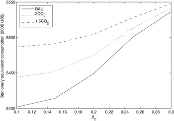
Figure 6 demonstrates the dependence of welfare on β2. The figure's qualitative features are easily explained. As β2 increases, the welfare differences between the three mitigation scenarios decrease. This is so since high values of β2 correspond to cases in which adaptation is highly effective at reducing damages. For these values, adaptation is so effective that only small adaptive investments are required to reduce damages substantially (in fact, to near zero for β2 ≈ 0.3). Hence the higher temperatures that correspond to weaker mitigation scenarios are of little consequence for welfare. For low values of β2, however, welfare is heavily dependent on the mitigation scenario.
Dependence of welfare on β2

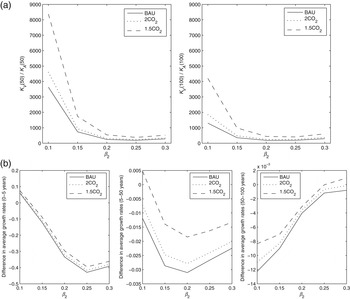
The fact that β2 has such a strong effect on the damage-moderating ability of adaptive capital leads to some interesting results for the dynamics of the capital stocks. Figure 7a plots the capital ratio as a function of β2 – unsurprisingly, these ratios are decreasing in β2, as an increase in β2 makes adaptive capital more effective, thus encouraging adaptive investment and decreasing the capital ratio. More interestingly, figure 7b demonstrates that, unlike the parameters discussed in section 3.3.2, low values of β2 can qualitatively alter the dynamics of capital accumulation. The left panel in figure 7b shows that for low β2, vulnerable capital grows faster than adaptive capital at early times (the first five model years). Figure 8 plots the full time series of the capital ratio for the low value β2 = 0.1, showing the early period in which vulnerable capital grows faster than adaptive capital, before declining into the U-shape familiar from figure 2.
Dependence of optimal capital trajectories on the effectiveness of adaptation (β2): (a) dependence of capital ratio on effectiveness of adaptation (β2), after 50 (left panel) and 100 (right panel) years, respectively; (b) difference between the average growth rates of vulnerable and adaptive capital, as a function of β2, for model years 0–5 (left panel), 5–50 (middle panel) and 5–100 (right panel)

Capital ratio for the low value β2 = 0.1. For this value of β2 it is optimal to engage in a brief period in which ‘development’ investments are favoured before building up adaptive capital stocks

Initial stock of adaptive capital
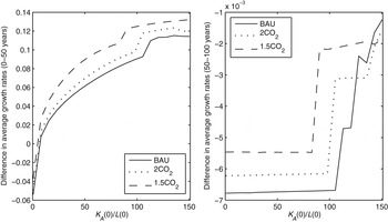
All of our sensitivity analyses thus far have investigated the effects of perturbations to the parameter values assumed in our base case model runs, i.e., they hold the control problem the planner faces fixed, but vary some of its structural parameters. It is also interesting to ask how the results change if we hold the parameters fixed, but vary the control problem by changing the initial conditions. In figure 9 we plot the dependence of the difference in the average growth rates of vulnerable and adaptive capital as a function of the initial stock of adaptive capital K A (0).Footnote 8
Difference between the growth rates of vulnerable and adaptive capital, as a function of the initial stock of adaptive capital per capita K A (0)/L(0), after 50 (left panel) and 100 (right panel) years

The figure shows that changing the value of K A (0) can change the qualitative features of capital accumulation, with higher values of K A (0) giving rise to a higher growth rate in the vulnerable sector than the adaptive sector over the first 50 years. This result reflects the fact that the marginal productivity of adaptive capital is decreasing in the capital stock. However, even for large values of K A (0), adaptive capital grows faster than vulnerable capital over the second 50 years.
The value of K A (0)/L(0) and the value of β2 jointly determine the initial marginal productivity of the adaptive sector. We have shown that low values of β2 and high values of K A (0)/L(0) can lead the vulnerable sector to grow more quickly than the adaptive sector initially. Which values of these parameters are most plausible? While the empirical evidence necessary to tightly constrain the value of β2 is not currently available, we stress that we consider the lowest values of K A (0) to be the most empirically relevant. Recall that adaptive capital in our model has no productive benefits unless the climate changes, i.e., X > 0. With this definition in mind, it seems very unlikely that sub-Saharan Africa has anything more than a nominal stock of adaptive capital at present. Although there are many capital items currently in place that help reduce vulnerability to current climate variability, these do not count as adaptive capital in our model. Thus, for example, a sea wall designed to protect against storm surge does not contribute to adaptive capital unless it is built higher than it would have been to optimally cope with existing climatic conditions. Only that portion of a wall that is beneficial if the sea level rises counts as adaptive capital. The National Adaptation Programme of Action country database produced by the UNFCCC,Footnote 9 which collates proposed national adaptation projects, shows that, even if we optimistically assume that all the proposed projects are currently in existence, the resulting estimates of current adaptive capital stocks are very low. For example, Zambia proposed adaptation projects valued at approximately US$ 13 million. Since Zambia's population is also approximately 13 million, this corresponds to US$ 1 per capita of adaptive capital if all the proposed projects were currently in existence, assuming all the installed capital is exclusively adaptive. The optimism of these assumptions means that lower values are much more likely. Moreover, there is much evidence to suggest that sub-Saharan African countries lack capital to deal even with current climate variability. For example, a well-known statistic is that Ethiopia has just 1 per cent of the artificial water storage capacity per capita of North America, despite enduring far greater hydrological variability (World Bank, 2006b). Overall then, we believe that very low values of the initial adaptive capital stock are most plausible.
4. Discussion
Our model offers a simple theoretical framework for investigating optimal investment in adaptive capital. It aims to make the sensitivity of policy recommendations to key assumptions clear and transparent. We show which parameters are most important in determining the qualitative features of the solutions, and why they affect the results as they do. Many of the key parameters of the adaptation problem are highly uncertain, so precise quantitative policy prescriptions are likely to be out of reach, thus heightening the importance of a qualitative understanding of the dynamics of successful adaptation.
Our analytical results showed that adaptive investment is positive when temperatures are increasing, even when the vulnerable sector is growing, thus arguing against the strongest version of the ‘adapt through development’ position. We also investigated the rate of response of the adaptive investment rule to climate change across different levels of economic development, where development is measured by the stock of vulnerable capital. We showed that whether or not rich (poor) economies have a stronger (weaker) proportional response to a change in temperature depends on whether the elasticity of the damage multiplier with respect to temperature is higher than its elasticity with respect to adaptive capital. This is a complex condition, which depends on the parametric form of the damage multiplier, as well as the stock of adaptive capital and magnitude of temperature change. Existing empirical results cannot determine whether this condition is satisfied for all time, so it is not clear {a priori} that wealthier (poorer) economies have less (more) need for adaptive investment. Thus, we conclude that the problem of optimally allocating investment between vulnerable and adaptive capital is not a simple matter, and deserving of careful analysis beyond the at times {ad hoc} recommendations in the existing literature.
In order to progress beyond these suggestive analytical results, we proceeded to make an empirical application of the full version of our model – with exogenously evolving technology and labour, and adjustment costs – to sub-Saharan Africa. Our base case results show that even relatively small investments in adaptive capital bring about large welfare benefits, especially in the more extreme climate change scenarios. We also find that it is optimal to grow the stock of adaptive capital more rapidly than vulnerable capital early on, although the adaptive sector never exceeds 1 per cent of the economy. This result reflects the fact that returns are greater in the adaptive sector than the vulnerable sector when the adaptive capital stock is low – in part due to the concavity of the production functions in each of these sectors, but also in part due to the persistent benefits of adaptive capital over time, and the need to make anticipatory adaptive investments so that the stock of adaptive capital is high when temperatures are at their peak.
In order to investigate the robustness of these results to our parameterization of the model, we conducted sensitivity analysis over key parameters – the climate sensitivity and CO2 stabilization scenario, the costs of adjustment, the rate of growth of TFP, the effectiveness of adaptation, the discount rate and elasticity of marginal utility, and the initial stock of adaptive capital. We found that, in almost all cases, and over plausible ranges for the relevant parameters, our central finding that the rate of growth of adaptive capital exceeds that of vulnerable capital at early times is preserved. Although our sensitivity analysis was not exhaustive (a practical impossibility given the high dimensionality of the parameter space in even our simple model), we focussed on the most important parameters for the problem at hand. Other parameters such as the coefficients and exponent of the gross damage multiplier, the capital share of production, and labour time series, clearly affect the model results too; however, their effects on the economic dynamics are partially mimicked by our existing sensitivity analysis. For example, changes to α1 and α2 in the damage multiplier would have similar effects to changes in the climate sensitivity S, the mitigation scenario and the effectiveness of adaptation β2.
The only parameters able to disturb our main finding of rapid growth in the adaptive sector were β2, the exponent of adaptive capital in the residual damage function, and the value of the initial stock of adaptive capital. β2 controls the effectiveness – i.e., the damage-reducing ability – of the stock of adaptive capital. If β2 is low, it is optimal to grow the stock of vulnerable capital rapidly for a brief initial period, before once again investing heavily in adaptive capital. Large initial stocks of adaptive capital mean that the effects of decreasing returns are felt more strongly, making adaptation a less attractive investment relative to vulnerable capital. However, we have argued that current stocks of adaptive capital are likely to be very low in most developing countries. From this analysis we conclude that β2 is perhaps the most crucial uncertain parameter in the model, as it is poorly constrained by the empirical literature, and has a major effect on the qualitative dynamics of the optimal capital accumulation paths. In general, efforts to quantify the structural relationship between the value of the adaptive capital stock and reductions in climate damages should be priorities for empirical work.
Our model could be extended in several directions. Clearly, economic modelling of adaptation planning would be immeasurably improved by better empirical estimates of the costs and benefits of adaptation, however difficult this exercise is. An assumption in our model deserving of further analysis is that adaptive capital is more effective at damage reduction at high temperatures than at low ones. As a first pass at the problem of modelling the effects of adaptation, this is an intuitive assumption. However, it may not hold at all temperatures – if climate change is severe enough, the marginal unit of adaptive capital may have little impact on damages. This reasoning suggests that there may be threshold effects that moderate adaptive investment strategies,Footnote 10 but the nature of such thresholds is very poorly understood. A further important extension of our model would take into account learning effects. Our results are analogous to those of Nordhaus (Reference Nordhaus2008) in the mitigation literature, who also solves deterministic control problems with sensitivity analysis over the solutions, rather than to the stochastic dynamic programming approach in, e.g., Kelly and Kolstad (Reference Kelly and Kolstad1999) (in which optimal policies account for uncertainty and learning effects).
Supplementary materials and methods
The supplementary material referred to in this paper can be found online at journals.cambridge.org/EDE/.