1 Introduction
Preferences are involved in many problems in computer science. People who have complex decisions to be made can be assisted by decision-support systems, where such decisions must be made based on the preferences of a particular individual. Similarly, the information provided by the Web is massive, and even with search tools it can be hard to find needed information in a timely fashion because this will typically provide very many website URLs as a result; here, preferences can be helpful in restricting and ranking the results. These different scenarios illustrate the relevance of research on preferences to different research areas, such as artificial intelligence (AI) and databases. As a consequence, a large number of approaches for dealing with preferences have been proposed, with the general goal of aiding users in making decisions, either when they are unsure about which choice to make due to, for example, uncertain outcomes, or when they cannot demand enough time and effort to analyse all the available options. While new approaches are typically compared with existing ones within the same research area, there is typically limited investigation of the relationship of such approaches across different areas.
This notion of research area is only one of the dimensions in which preference-related work can be categorised. A second dimension is the kind of preferences that different approaches deal with. Here, preferences are typically classified as qualitative (e.g. I like oranges more than apples) or quantitative (e.g. I rate this movie with five stars), where the former is closer to how people express preferences than the latter. In addition, observing a third dimension, work on preferences investigates different problems (Brafman & Domshlak, Reference Brafman and Domshlak2009), such as: (i) preference elicitation and learning: how to obtain preferences from users (Hudson & Sandholm, Reference Hudson and Sandholm2004; Luo et al., Reference Luo, Jennings and Shadbolt2006; Pu & Chen, Reference Pu and Chen2008; Hu & Pu, Reference Hu and Pu2009; Fürnkranz & Hüllermeier, Reference Fürnkranz and Hüllermeier2011); (ii) preference representation: how to provide syntax (language) and semantics (model) to represent preferences (Ayres & Furtado, Reference Ayres and Furtado2007; Nunes et al., Reference Nunes, Barbosa, Cowan, Miles, Luck and de Lucena2013); and (iii) preference reasoning: how to use preferences for making decisions, ordering search results, and other purposes (Domshlak, Reference Domshlak2008). In this paper, we fix two of these dimensions—the kinds of preferences and the investigated problems—and explore approaches proposed in the context of different research areas.
In presenting a survey of approaches to reasoning about qualitative multi-attribute preferences, we have selected approaches, from different research areas, that propose techniques and algorithms, and which take as input qualitative preference statements following a particular structure specified by the approach. Other approaches out of the scope of the paper have been proposed, but they are generally either an alternative way of reasoning about the same kinds of statements as those processed by the approaches introduced here, or propose extensions to these approaches, sometimes increasing their power of expressivity. Although we do not cover such extensions, by introducing our selected approaches we provide the knowledge needed to understand their extensions. In addition, there is significant amount of work on qualitative preference reasoning that, instead of offering algorithms or computational techniques, provides new logics and logic frameworks. These approaches are also left out of the scope of the paper, because we focus on more practical approaches, rather than purely theoretical ones. Furthermore, existing surveys and books on this particular topic are available elsewhere (Delgrande et al., Reference Delgrande, Schaub, Tompits and Wang2004; Kaci, Reference Kaci2011).
The key goal of this review is to provide a clear overview of the different approaches and determine how they differ with respect to qualitative preference reasoning, so that researchers can understand the main aspects of this particular research area (i.e. qualitative preference reasoning), identify those approaches that are better at solving specific problems, and combine those approaches that may be complementary. As this problem area is investigated from the perspective of many research areas, our aim is to allow researchers to identify potential synergies that can be explored across research areas. There are surveys (Walsh, Reference Walsh2007; Domshlak, Reference Domshlak2008; Brafman & Domshlak, Reference Brafman and Domshlak2009; Domshlak et al., Reference Domshlak, Hüllermeier, Kaci and Prade2011) that give overviews of work on preferences in AI or qualitative preferences, but they focus on a broad brush presentation of these research topics, and provide many pointers to existing work. In contrast, this paper provides a comprehensive review of approaches to qualitative preference reasoning, so that it is possible to understand their key aspects; that is, the kinds of issues they address, which structures they use as input, how they work, and their limitations. This helps to identify those approaches that are applicable to solve particular problems and the limitations to be addressed, without requiring the reader to understand all of their complex details and the algorithms used. This paper thus serves as an introduction to the field of qualitative multi-attribute preference reasoning, and gives the foundation needed to understand much state-of-the-art research that relies on the work presented here.
We begin by describing the evaluation framework adopted to analyse each investigated approach in Section 2. Before introducing them, we first provide some background on Multi-Attribute Utility Theory (MAUT, Section 3), which is one of the oldest tools to help decision makers make choices, and which inspired much of the existing work on reasoning about preferences in different research areas. Although it deals with quantitative preferences (which are out of the scope of this paper), it specifies concepts that are adopted in the majority of what is discussed here. The different approaches are then presented from Sections 4 to 7, organised in the following way. The first group we present consists of those based on utility functions (Section 4), using specific (logic-based) languages to represent qualitative preferences and forms to derive utility functions from these models. Those detailed in Section 5 take another direction: they adopt new graphical structures to represent and reason about preferences. Next, Section 6 describes approaches that represent preferences with constraints, and extend constraint satisfaction problems (CSPs) to incorporate soft constraints, that is, constraints that can remain unsatisfied. Finally, databases are another research area in which preferences have been investigated, and work in this area is presented in Section 7. These database approaches develop extensions of query languages to incorporate preferences and algorithms to provide query results taking the specified preferences into account. After presenting all of these approaches, we discuss them and their applications, and show how they are related in Section 8, and we conclude in Section 9.
2 Review method
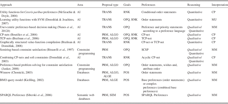
Our comparison of the different approaches to reasoning about multi-attribute qualitative preferences follows an evaluation framework composed of six different criteria, which are described below. For each approach, this information is compiled into a table, each of which we refer to as reference card.
Proposal type.What is the approach proposing? Many approaches have the goal of answering user questions that are related to preferences and decision making (see goals in the next criterion), so they propose preference representation models (possibly with an associated language), and/or algorithms to answer those questions. Other approaches start from an existing (lower-level) preference representation model that has associated algorithms to answer the questions, and provide a means of transforming high-level preference models into low-level ones. Therefore, for this criterion, we classify approaches according to the following proposal types: (i) preference representation models; (ii) algorithms, algebras, or semantics to answer preference-related questions or interpret preference constructions; and (iii) X to Y transformation, that is, transform preferences represented in a model X to preferences represented in a model Y.
Goals.Which preference-related questions are addressed by the approach? As stated above, many approaches aim to answer preference-related questions, so when the approach has this as an explicit goal, we show which questions are addressed by each. The types of questions answered by work covered in this paper are detailed below.
∙ Optimisation queries: what are the k-optimal options according to the given preferences? In the presented approaches, k=1, unless otherwise stated.
∙ Ranking queries: what is the ranking that orders options from best (most preferred) to worst (least preferred), according to the given preferences?
∙ Pareto-optimal set identification: what are the maximal (non-dominated) options according to the given preferences?
Note that some approaches may answer such questions indirectly. For example, if an approach proposes transforming a logic-based preference language into utility functions, it allows the (indirect) answering of those questions that can be answered with utility functions.
Input.What is the input required by the approach? If the approach relies on a particular structure, specific to the approach, we provide details.
Interpretation.What interpretation is adopted for preference statements? Most approaches use preference statements (or a particular representation of them) as input, but they can be interpreted in different ways, and we classify them into two categories. The first is ceteris paribus (Hansson, Reference Hansson1996), which means ‘all else being equal’. Here, if one states ‘I prefer value v 1 to value v 2 with regard to attribute x’, it means that this preference can be considered only when the values of all other attributes are equal. Of the possible interpretations, the other used by the approaches discussed in this paper is mutatis mutandis, which means ‘with the necessary changes having been made’. In this case, when a preference is provided, it is applied to any context. For example, if one states that ‘lowest’ price is a preference for cars, then any cheaper car is preferred to any more expensive car.
Complexity.What is the complexity of the proposed algorithm? Some approaches do not provide a complexity analysis, so this criterion is not specified for them.
Limitations.What are the limitations of the proposed approach? Different approaches may have limitations in different aspects, such as having algorithms that take exponential time to be executed or preferences expressed in ways that are hard to elicit.
In addition to providing a reference card for each approach, we also explain how it works. This explanation further details the required input, if necessary, and how the preference reasoning works. Our goal is to give only a broad understanding of each approach, rather than an extensive description of the algorithms involved and all their steps.
3 Background: Multi-Attribute Utility Theory
MAUT is a set of methods designed to handle decision problems involving multiple objectives and trade-offs. According to Dyer (Reference Dyer2005), MAUT has become synonymous in the view of many scholars with the theory proposed by Keeney and Raiffa (Reference Keeney and Raiffa1976), which emphasised the use of multi-attribute preference models based on the theories of Von Neumann and Morgenstern (Reference Von Neumann and Morgenstern1944), who presented a set of axioms about preferences and utilities such that any decision maker satisfying these axioms has a utility function.
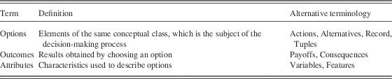
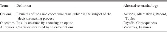
MAUT is concerned with the valuation of the outcomes of an option of a decision maker. In this context, a problem is described in terms of attributes X={x 1, … , x n}, which can have values assigned according to their respective domains D 1, … , D n, establishing the range of possible values of an attribute. The set of all possible outcomes is the Cartesian product of attribute domains D 1× … ×D n. Feasible outcomes are a subset of all possible outcomes, and are those that consist of valid combinations of attribute values. Now, a (cardinal) utility function is a function that maps outcomes to real values that represent the preference for each outcome. The higher the value, the more preferred the outcome. In Table 1, we give the definition of the three main terms (option, outcome, and attribute) adopted in MAUT and decision making, introduced above, together with alternative terminology, as different approaches sometimes use different terms. In some cases, options lead to only one possible outcome, and here the terms option and outcome are used as synonyms; for example, choosing a product (option) A to be bought leads to the single consequence of buying the product (outcome), so A can be used to refer to both the option and the outcome.
Main terms adopted in decision making
Keeney and Raiffa (Reference Keeney and Raiffa1976) discuss decisions that can be made under certainty or uncertainty. The former refers to situations in which the outcome, represented by multiple attributes, of an option is known. In these scenarios, the main challenge is to resolve trade-offs among preferences, which typically conflict because in general they cannot be maximised at the same time. For instance, two preferences might seek to maximise quality and minimise costs, but lower costs are normally achieved by compromising quality. In the latter—that is, the cases in which uncertainty is present, or in other words risky situations—outcomes depend on an occurrence from a set of events. Note that decisions under risk and under uncertainty are sometimes not considered synonymous, as some authors consider decisions under risk to be those for which there is a probability associated with the outcomes, and decisions under uncertainty to be those for which it is not possible to list all outcomes or the probabilities are unknown. In this paper, we do not consider this latter case, following Keeney and Raiffa (Reference Keeney and Raiffa1976).
A preference representation function under certainty is referred to as a value function v, which associates a real number with each point x in the outcome space, representing the preference structure of the decision maker, provided that
 $$\forall x',x''\in D\,x'\,\sim\,x'' \Leftrightarrow v(x')=v(x'')\,and\,x'\,{\succ}\,x'' \Leftrightarrow v(x')\,\gt\, v(x'')$$
where ~ and ≻ represent indifference and preference, respectively. Based on v, the goal is to find an outcome x∈D to maximise v(x).
When the decision making is based on the assumption of the existence of value functions, two concepts (preference independence and mutual preference independence) play an important role, as they are related to properties of the value function, and can facilitate its elicitation process. The definitions of these two concepts are given below.
Preference independence. An attribute set Y, where Y⊂X, is preferentially independent of its complement  $\bar{Y}$
if the preference order of two outcomes involving different values assigned to Y does not depend on the fixed values assigned to attributes in
 $\bar{Y}$
. For example, if a laptop colour is preferentially independent of the remaining laptop attributes, and one states that they prefer silver to black then, by fixing the values of the remaining attributes, any silver laptop is preferred to any black laptop.
Mutual preference independence. The attributes x 1, … , x n are mutually preferentially independent if every subset Y of X is preferentially independent of its complementary set.
Mutual preference independence is a key condition to allow value functions to be represented using an additive form, which is the most common approach for evaluating multi-attribute alternatives. In this representation, attribute values are considered independent, and therefore the value of an outcome can be calculated by adding the values of individual attributes. This form of value function is as follows, given the attributes x 1, … , x n:
 $$v\left( {x_{1} ,x_{2} ,\,\,\ldots\,,x_{n} } \right)\!=\!\mathop{\sum}\limits_{i=1}^n {v_{i} \left( {x_{i} } \right)} $$
where the v i are consistently scaled single-attribute value functions.
Moreover, if we consider trade-off among attributes, represented by weights w i, we have the following additive value function:
 $$v\left( {x_{1} ,x_{2} ,\,\,\ldots\,,x_{n} } \right)\!=\!\mathop{\sum}\limits_{i=1}^n {w_{i} v_{i} \left( {x_{i} } \right)} $$
where w i>0 and  $$\mathop{\sum}\nolimits_{_{i} _{{={\rm 1}}} }^n {\;w_{i}\!=\!{\rm 1}} $$
.
This additive decomposition of a value function can be generalised as generalised additive independence models, in which factors are overlapping subsets of attributes, instead of single attributes, leading us to the generalised additive (GA) form (Fishburn, Reference Fishburn1982; Bacchus & Grove, Reference Bacchus and Grove1995). Considering (generalised) additive independence is ideal because it leads to compact models, as a particular value does not need to be specified for each possible outcome, and the number of which is exponential in the size of attribute domains. In this paper, we adopt the term compact as an adjective for approaches which, with little information (preference statements, utility values), one can still derive a preference order between two outcomes.
When uncertainty is considered, the preference representation function is referred to as a utility function u, in which risky options are defined as lotteries or gambles with outcomes that depend on an occurrence from a set of mutually exclusive and exhaustive events (Dyer, Reference Dyer2005). We now introduce concepts related to decisions under this kind of scenario—many of these definitions come from the formalisation of expected utility theory by Von Neumann and Morgenstern (Reference Von Neumann and Morgenstern1944).
∙ A lottery is any option with an uncertain outcome. Examples are investment, roulette, or a game of football.
∙ The probability of an outcome (of a lottery) is the likelihood that this outcome occurs. The probability is often estimated by the historical frequency of the outcome.
∙ The probability distribution of the lottery depicts all possible outcomes in the lottery and their associated probabilities. The probability of any particular outcome is between 0 and 1, and the sum of the probabilities of all possible outcomes is equal to 1.
The definitions of (mutual) preference independence are then extended by considering uncertainty: an attribute x i is said to be utility independent of its complementary attributes if preferences over lotteries with different values of x i do not depend on the fixed values of the remaining attributes. Attributes x 1, x 2, … , x n are mutually utility independent if all proper subsets of these attributes are utility independent of their complementary subsets.
Once utility functions are correctly defined for a decision maker, typical preference-related tasks such as comparing and ranking outcomes, can be easily performed and questions answered, as they require only a numerical comparison. Therefore, MAUT does not focus directly on algorithms to answer questions related to preference reasoning, but on revealing the value or utility function of decision makers. As a consequence, the main difficulty related to MAUT is the elicitation process of these quantitative preferences, which is often tedious and requires user effort. Qualitative preferences, on the other hand, make this process easier by capturing preferences in a language or model closer to that of users, which is more intuitive, and the approaches that handle this kind of preference are those discussed in this paper.
4 Utility function-based approaches
In this section, we present approaches that use utility functions to reason about preferences for which, as discussed above, the main challenge is to identify the utility function of the decision maker—in our case, the user. As our focus is not the elicitation process, we do not describe here those approaches that reveal utility functions by means of user interaction. The three approaches presented in this section propose algorithms and methods to transform qualitative preference statements into a utility function, with which it is possible to derive an ordering over options, and consequently to identify the optimal option. We remind the reader that, for each approach, we provide a reference card with the items detailed in Section 2 and describe how it works.
Some authors might argue that such approaches should be understood as being kinds of preference learning. However, according to Fürnkranz and Hüllermeier (Reference Fürnkranz and Hüllermeier2011), ‘preference learning is about inducing predictive preference models from empirical data’, and these approaches receive as input structured data.
4.1 Utility functions for ceteris paribus preferences
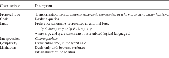
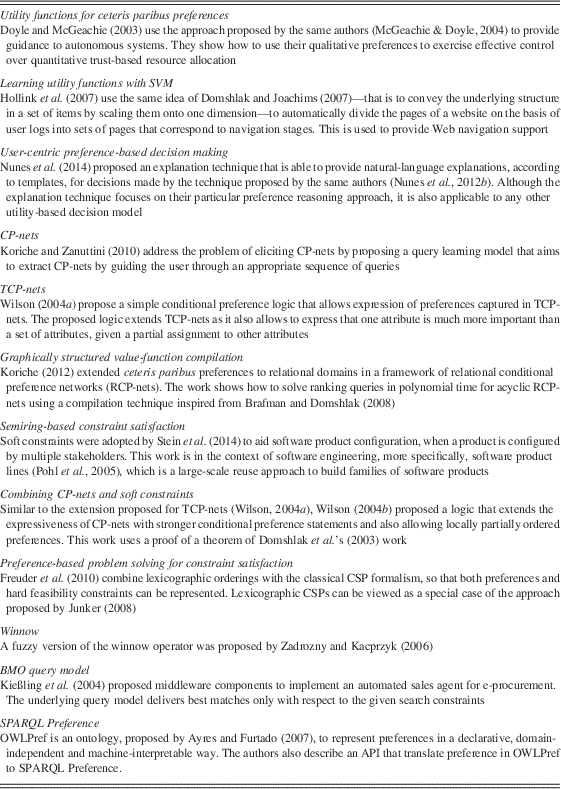
McGeachie and Doyle (Reference McGeachie and Doyle2002, Reference McGeachie and Doyle2004) present a set of methods for translating preference information from a qualitative representation to a quantitative representation, summarised in Table 2. Broadly, they consider ceteris paribus preferences, represented with a propositional language augmented with an ordering relation that is used to express preferences over propositional combinations of a set of elementary attributes. This qualitative representation is then converted to an ordinal utility function to be used in reasoning processes.
Reference card: utility functions for ceteris paribus preferences
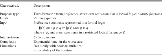
In order to specify a set of possible options, a restricted logical language  $$ \cal L $$
is adopted, using only two logical operators: ¬ (negation) and ∧ (conjunction) to construct finite sentences over a set of atoms, each corresponding to an attribute from a space of binary attributes describing possible worlds. A complete consistent set of literals is a model. For example, cars may be defined in terms of four attributes, sportType, SUVtype, yellow, and red. Based on these attributes, we specify a set of four possible models below.
∙ m 1: sportType, ¬SUVtype, yellow, ¬red (yellow sport cars);
∙ m 2: sportType, ¬SUVtype, ¬yellow, red (red sport cars);
∙ m 3: ¬sportType, SUVtype, yellow, ¬red (yellow SUV cars);
∙ m 4: ¬sportType, SUVtype, ¬yellow, red (red SUV cars).
Based on this, we can specify ceteris paribus preferences: where p and q are statements in  $$ \cal L $$
: p ⊵ q, when p is desired at least as much as q (formally, it is interpreted that p∧¬q is desired at least as much as q∧¬p); and p ⊳ q, when p is strictly more desired than q. Moreover, conditions may also be specified, in the form if r then p ⊵ q, meaning that the ceteris paribus preference holds, if r (also a statement in
 $$ \cal L $$
) holds. For example, conditional ceteris paribus preferences may be: if sportType, then red ⊳ yellow and if SUVtype, then yellow ⊳ red. This means that in the cases where sportType holds, that is, m 1 and m 2, red is strictly more preferred than yellow, all else being equal; and in the cases where SUVtype holds, that is, m 3 and m 4, yellow is strictly more preferred than red, all else being equal (but in this example there are no other attributes).
Based on specified preferences, the goal is to derive a preference order, which is a complete preorder (reflexive and transitive relation) ≿ over the set of all models of  $$ \cal L $$
. When, given two models m and m′, m ≿ m′, it is said that m is weakly preferred to m′. If m≿m′ and m′≵m, it is said that m is strictly preferred to m′, written m≻m′. If m≿m′ and m′≿m, then it is said that m is indifferent to m′, written m~m′. For instance, if we consider the preference specified above (if sportType, then red ⊳ yellow), then we can conclude that m 2≻m 1.
In order to do so, the general idea of the approach is to generate an ordinal utility function from a set C of ceteris paribus preferences over attributes X. An initial step is performed, which translates the provided statements represented in a logical representation of ceteris paribus preferences to an attribute-vector representation. The latter is then used to produce the utility function in the following way. The structure of preference statements in the attribute-vector representation is used to infer additive utility independence among attributes. Next, subutility functions are defined for each utility-independent set of attributes—if no utility independence was identified in the previous step, only one subutility function, associated with the set of all attributes, is defined in this step. This is done based on the representation of preorders consistent with the preferences by building a graph over assignments to the attributes. Finally, to assign relative weights of satisfaction of different attributes (i.e. to establish trade-offs among attributes), a linear programming problem is solved. In the end, a utility function that can be used to evaluate the utility of different assignments to values of X is built.
This work has two different aspects related to complexity, which are associated with (McGeachie & Doyle, Reference McGeachie and Doyle2004): (i) the time and space required to construct the utility function u and (ii) the time and space required to evaluate u(m) on a particular model m. Both take exponential time, in the worst case. Constructing u involves solving a satisfiability problem, where the time required depends on the number of rules involved in conflicts in each utility-independent set. On the other hand, computing u(m) involves computing u i(m), where u i is a minimising utility function, for all the utility-independent attribute sets. Each of the subutility functions can be exponential in the size of the utility-independent set.
4.2 Learning utility functions with support vector machine
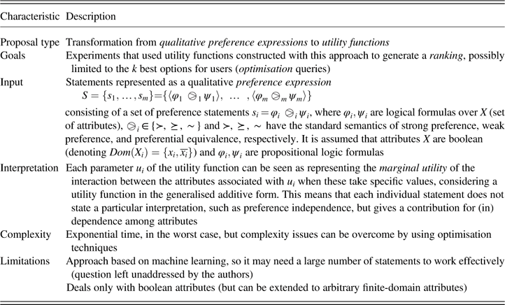
The approach proposed by Domshlak and Joachims (Reference Domshlak and Joachims2006, Reference Domshlak and Joachims2007) takes a new direction for reasoning about preferences, as introduced in Table 3. First, it adopts a new form of representing preferences: instead of seeing an option as a set of values (parameters) specified for a set of attributes, it linearises the possible combinations of attribute values and each of these combinations is seen in a unified non-parametric way, that is, as a unique specification. For instance, ‘big red suitcase’ is not an option (suitcase) parameterised with values assigned to colour and size, but as a single option. Second, machine learning techniques are adopted to generate a utility function to model user preferences. Preferences are represented as qualitative preference expressions, as detailed in Table 3.
Reference card: learning utility functions with SVM

SVM=Support vector machine.
The two main aspects of this work are the proposed underlying preference representation, that is, how the qualitative preference statements are represented, and how the utility function is generated. The situation explored in this work is when the system cannot assume a significant independence structure on attributes. So, the basic idea is that if no useful preference independence information in the original representation space is provided, a different space is adopted in which no such independence information is required. This new space is specified as follows: assuming that the attributes X are all binary valued, there is a mapping from the options χ into a new, higher-dimensional space  $$ \cal F $$
using a certain mapping Φ=χ ↦
 $$ \cal F $$
=ℝ4n.
The mapping Φ is not arbitrary, but establishes a connection between the dimensions χ and  $$ \cal F $$
, in which each element of
 $$ \cal F $$
is a combination of values of attributes. Explaining Φ formally is outside the scope of this paper, so we limit ourselves to an informal example. Consider two attributes to describe a car: sport type (with values sportType and ¬sportType) and colour red (with values red and ¬red). The mapping Φ maps an option o=〈sportType, ¬red〉 to a value 1 when sportType or ¬red holds, or both, and to a value 0, otherwise, as shown below:
 $$\qquad \qquad \qquad \qquad \qquad \qquad \quad \qquad \Phi \left( x \right)=\matrix{ {\matrix{ {\left[ {\matrix{ 1 \cr 0 \cr 0 \cr 1 \cr 0 \cr 1 \cr 0 \cr 0 \cr } } \right]} & {\matrix{ \hskip -33pt { & sportType} \cr \hskip -26pt { & \neg sportType} \cr { \hskip -59pt & red} \cr { \hskip -52pt & \neg red} \cr { \hskip -11pt & sportType,\,\,red} \cr { & \hskip -5pt sportType,\,\neg red} \cr { & \hskip -4pt \neg sportType,\,\,red} \cr { & \hskip 2pt \neg sportType,\,\,\neg red} \cr } } \cr } } & \eqalignno{ & \cr & \cr & \cr & \cr & \cr & \cr & \cr & \cr} \cr } $$
Note that there are also dimensions not shown here, with three or four elements, but they are all 0 because they include either sportType and ¬sportType, or red and ¬red.
Any preference ordering over χ is additively decomposable in  $$ \cal F $$
; that is, weights w i can be associated with Φ(x)[i], so that they are in accordance with provided preference statements. Consequently, statements are used as constraints over weights together with an objective function in an optimisation problem. To calculate weights, techniques frequently used in machine learning in the context of support vector machines (SVMs) (Vapnik, Reference Vapnik1998) are adopted, as this mapping of inputs into high-dimensional attribute spaces, called the kernel trick, is used in SVM to perform a nonlinear classification.
Solving the optimisation problem of this approach raises several complexity issues. First, although this constraint system is linear, it is linear in the exponential space ℝ4n. Second, the description size of the optimisation problem and, in fact, of each individual constraint of it, can be exponential in n. Nevertheless, Domshlak and Joachims (Reference Domshlak and Joachims2007) show that these complexity issues can be overcome using optimisation techniques and some assumptions, such as that propositional formulas coming from user statements are unlikely to be of a size that would pose computational challenges in practice.
This work is strongly associated with machine learning (Alpaydin, Reference Alpaydin2010; Flach, Reference Flach2012) and recommender systems (Adomavicius & Tuzhilin, Reference Adomavicius and Tuzhilin2005; Su & Khoshgoftaar, Reference Su and Khoshgoftaar2009; Ricci et al., Reference Ricci, Rokach, Shapira and Kantor2011). It interprets each pairwise comparison as likes and dislikes of options with similar values for attributes and builds a model that generalises these comparisons, which can also be with the whole set of options, when monadic statements (those with a single referent, such as I like red) are provided. Therefore, there is a statistical generalisation and, to achieve good results here, a large number of statements may be needed. This is reflected in the future work reported by the authors, whose goal is to specify the number of preference statements that a user must provide to infer a utility function that is effective.
4.3 User-centric preference-based decision making
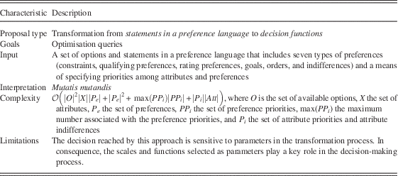
Nunes et al. (Reference Nunes, Miles, Luck and Lucena2012a, Reference Nunes, Miles, Luck and Lucena2012b) proposed a preference reasoning technique (detailed in Table 4) whose goal is to simulate human reasoning in making decisions, allowing exploitation of natural user expressiveness of preferences (without the need for elicitation methods) and resolve trade-offs (that cannot be resolved with the provided preferences) in the way that humans would do so. As a result, the technique is based on heuristics investigated in psychology that explain how people make decisions.
Reference card: user-centric preference-based decision making
The input of the technique consists of a set of options over which a choice is made, and a set of preferences expressed in a language—derived from a study of how humans express preferences (Nunes et al., Reference Nunes, Barbosa, Cowan, Miles, Luck and de Lucena2013)—that allows the construction of statements such as those shown below. This is an example in a scenario in which a choice for an apartment is being made by a student, where apartments are described in terms of zone (the zone in which the apartment is located), uni (distance from the apartment to the university), station (distance from the apartment to the underground station), and brand (the brand of the company to which the apartment belongs). Numbered statements are preferences over attribute values, while unnumbered statements are priorities over attributes. Numbers in preference statements indicate their priority: the lower the number, the more important the preference.
1. don’t acceptzone>2
2. preferuni⩽2.5 km
3. ifuni⩽2.5 km then requireprice⩽£125
4. ifuni>2.5 km then needstation⩽0.7 km
5. ifuni>2.5 km then requireprice⩽£105
6. minimisestation
7. minimiseprice
8. preferbrand=A orbrand=B orbrand=C
9. brand=A ≻ brand=B
10. brand=B ≻ brand=C
∙ ifuni>2.5 km thenstation ⊳ uni
The proposed technique processes preferences to select one option, in such a way that the choice, and the decision not to choose alternatives, can be justified by the preferences. The output is a partially ordered set, organised in four different levels: (i) the chosen option; (ii) acceptable options that are close to the chosen option, but not chosen; (iii) eliminated options, discarded because of a hard constraint; and (iv) dominated options. Heuristics used by humans are applied to make the choice, specifically reason-based choice (Shafir et al., Reference Shafir, Simonson and Tversky1998), which concerns how people make decisions by identifying reasons to accept and reject options, and the principles of trade-off contrast and extremeness aversion (Simonson & Tversky, Reference Simonson and Tversky1992), so that decisions more closely mirror user choices if users are provided with sufficient time and knowledge.
In outline, the steps of the technique are as follows. In the first step, pre-processing, options are analysed to extract the essential data. This includes how well option attributes meet the preferences, and how options compare with each other in relation to individual attributes. In the second step, explication, information that is implicit in the provided preferences is extracted and incorporated into the set of provided preferences. Next, the elimination step eliminates those options that do not meet strict constraints, or that are dominated in every respect by other options. Finally, the selection step makes the choice itself. Preferences and priorities are transformed into a quantitative decision function that can be seen as a relative utility function, which relates every two options. This relative utility function consists of three factors: the costs provided by the attribute values of an option with respect to another, the trade-off contrast, and extremeness aversion, these last two being heuristics people adopt in making decisions, determined using the costs.
Although this approach requires a relatively small amount of preferences to make a decision—that is, the preferences provided need not be sufficient to derive a partial order with an optimal option—due to the adoption of heuristics of human decision making, it has parameters (such as scales for natural-language keywords) that have a significant impact on the decision-making process.
5 Graphically structured approaches
As seen in the previous section, deriving a utility function from qualitative preference statements is a hard problem. To overcome this, some approaches take an alternative perspective. Instead of using mathematical or statistical mechanisms to reason about preferences, the approaches presented in this section propose new ways to represent preferences and relationships among attributes, together with algorithms that reason about preferences qualitatively. These representations, which rely on graph structures, have the goal of capturing preferences in an intuitive way and are also inputs to algorithms to reason about preferences.
5.1 Conditional preference networks
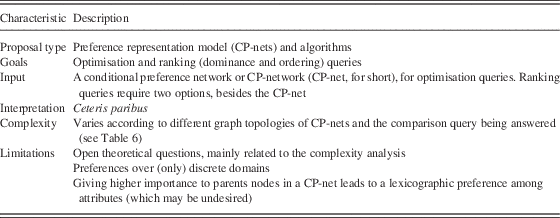
Conditional preference networks (CP-nets), the reference card for which is shown in Table 5, represent preferences in a compact graphical form and, according to Boutilier et al. (Reference Boutilier, Brafman, Hoos and Poole1999, Reference Boutilier, Brafman, Domshlak, Hoos and Poole2004) represent preference statements in a natural way. These statements are conditional qualitative preference statements interpreted under the ceteris paribus semantics.
Reference card: CP-nets
A CP-net over attributes X=x 1, … , x n is a directed graph G over x 1, … , x n whose nodes are annotated with conditional preference tables CPT(x i) for each x i∈X. Each CPT(x i) associates a total order  $${\succ}_{u}^{i} $$
with each instantiation u of x i’s parents Pa(x i)=U. In summary, the kinds of statements captured by CP-nets are those that establish order among attribute values, conditioned to values set to other attributes (parent attributes). Optimisation queries require only a CP-net as input, and optionally a partial assignment for attributes, while the required input for ranking queries is a CP-net N and two options o and o′.
As CP-nets are graphical structures, in order to provide a better understanding of them, we first introduce a simple example (Boutilier et al., Reference Boutilier, Brafman, Domshlak, Hoos and Poole2004) that expresses preferences over dinner configurations. This network, depicted in Figure 1(a), consists of two attributes S and W, for soup and wine, respectively. Fish soup (S f) is strictly preferred to vegetable soup (S v), while the preference between red (W r) and white (W w) wine is conditioned on the soup to be served: red wine is preferred if served with a vegetable soup, and white wine if served with a fish soup.
Example of a CP-net (Boutilier et al., Reference Boutilier, Brafman, Domshlak, Hoos and Poole2004). (a) Preferences for soup and wine. (b) Induced graph.
The semantics of a CP-net is defined in terms of the set of preference rankings that are consistent with the set of preference constraints imposed by its CPTs. Figure 1(b) shows the preference graph over options induced by the previously described CP-net. An arc in this graph directed from option o i to o j indicates that a preference for o j over o i can be determined directly from one of the CPTs in the CP-net.
CP-nets are used to answer both optimisation and ranking queries. However, ranking queries are split into two categories. (i) Dominance queries: is an option o preferred to another option o′? If so, it is said that o dominates o′ with respect to the given preference structure. (ii) Ordering queries: is an option o′ not preferred to another option o? If so, it is said that o is consistently orderable over o′ with respect to the given preference structure. Ordering queries are weaker than dominance queries, because by answering the latter we know whether o≻o′ holds, while by answering the former we only know whether o′⊁o holds, which does not imply that o≻o′ holds. Next, we briefly describe how each of the preference-related questions is answered using CP-nets.
Optimisation. In order to generate the optimal option of an acyclic CP-net, the network is swept from top to bottom, with the forward sweep procedure (Boutilier et al., Reference Boutilier, Brafman, Domshlak, Hoos and Poole2004), which constructs the most preferred option. It considers, in order to be more general, given evidence constraining possible options in the form of an instantiation y of some subset Y⊆X of the network attributes. The algorithm sets Y=y, and instantiates each x i∉Y in turn to its maximal value given the instantiation of its parents.
Ordering. For acyclic CP-nets, Boutilier et al. (Reference Boutilier, Brafman, Domshlak, Hoos and Poole2004) define a corollary that provides an algorithm to answer ordering queries. The corollary states that given an acyclic CP-net N and a pair of options o and o′, if there exists an attribute x i in N, such that: (i) o and o′ assign the same values to all ancestors of x i in N; and (ii) o assigns a more preferred value to x i than that assigned by o′ given the assignment provided by o (and o′) to the parents of x i, then N ⊭ o′≻o.
Dominance. Answering dominance queries is equivalent to the task of determining the existence of an improving (or worsening) sequence of attribute value flips with respect to the given CP-net. A sequence of improving flips from one option to another provides a proof that one option is preferred, or unpreferred, to another in all rankings satisfying the network. This task can be reduced to a special subclass of classical planning problems, and several techniques can be used in a generic search procedure for an improving flipping sequence.
CP-nets were investigated for use with different algorithms related to reasoning about preferences, and their complexity analysed with different graph topologies. Optimisation queries can be answered using the forward sweep procedure, taking time linear in the number of attributes. The complexity of two of the ranking queries (dominance and ordering) has been analysed for different graph topologies of CP-nets, which can be seen in Table 6 (Boutilier et al., Reference Boutilier, Brafman, Hoos and Poole1999, Reference Boutilier, Brafman, Domshlak, Hoos and Poole2004). These results are associated with boolean attributes, but it is claimed that the ordering results also hold for multi-valued attributes. Finally, given a CP-net N over n attributes and a set of complete assignments o 1, … , o m, ordering these assignments consistently with N can be done using ordering queries only, in time  $${\cal O}(nm^{2} )$$
.
Complexity analysis of CP-nets (boolean attributes)

CP-nets=Conditional preference networks.
It is also proved that ordering queries are answered with CP-nets with a directed acyclic graph topology in  $${\cal O}(n)$$
. However, the complexity of other queries or CP-net topologies, such as the general case, are left as open questions, which led to further investigations by other researchers (e.g. Goldsmith et al., Reference Goldsmith, Lang, Truszczynski and Wilson2005).
This work thus leaves different open theoretical questions, mainly concerned with the complexity analysis of other scenarios in which CP-nets are used to reason about preferences. In addition, CP-nets address the representation of preferences over discrete domains, but common preferences, such as price minimisation, cannot be directly represented. Moreover, this way of identifying optimal options with CP-nets first optimises parent attribute values, for later assigning values for their children. This leads to a lexicographic preference among attributes, which may capture trade-off situations in an inappropriate way. This issue is investigated in trade-offs-enhanced conditional preference networks (TCP-nets), presented in Section 5.2, which adds importance relations and conditional relative importance statements to the conditional ceteris paribus statements supported by CP-nets.
5.2 Trade-offs-enhanced conditional preference networks
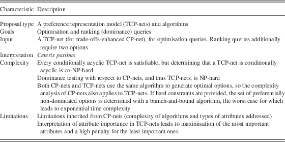
CP-nets represent the class of conditional qualitative preference statements. TCP-nets (Brafman & Domshlak, Reference Brafman and Domshlak2002; Brafman et al., Reference Brafman, Domshlak and Shimony2006)—for which the reference card is presented in Table 7—address a limitation of this approach by extending CP-nets to capture another class of preference statements: those with conditional relative importance. These statements have the following form: ‘it is more important to me that the value of x be high than that the value of x′ be high’. CP-nets can thus be extended with new types of arcs, in order to investigate questions to be answered based on this new graphical representation of preferences.
Reference card: TCP-nets
CP-nets=Conditional preference networks.
TCP-nets maintain the ideas of CP-nets, in that they remain focused on using only simple and natural preference statements, use the ceteris paribus semantics, and utilise a graphical representation of this information to reason about consistency and to perform, possibly constrained, optimisation. The extra expressiveness provided allows better modelling trade-offs, with attribute importance relationships. TCP-nets are annotated graphs with three types of edges:
1. a first type of (directed) edge comes from the original CP-nets model and captures direct preferential dependencies (shown as arrows from S to W and S to A in Figure 2);
2. a second (directed) edge type captures relative importance relations—the existence of such an edge from attribute x to attribute x′ implies that x is more important than x′ (shown as an arrow from D to S in Figure 2); and
3. a third (undirected) edge type captures conditional importance relations: such an edge between nodes x and x′ exists if there is a non-empty attribute subset Y⊆X−{x, x′} for which RI(x, x′|Y) (relative importance of x and x′ conditioned on Y) holds (shown as a line connecting W and A in Figure 2).
Example of a TCP-net
In addition to the CPT of CP-nets, in TCP-nets, each undirected edge is annotated with a conditional importance table (CIT). The CIT associated with such an edge (x, x′) describes the relative importance of x and x′, given the value of the corresponding importance-conditioning variables Y. A CIT is illustrated on the right-hand side of Figure 2.
We show an example of a TCP-net in Figure 2, which extends the CP-net example presented in the previous section, expressing preferences over dinner configurations. Besides specifying preferences for the attributes soup and wine (S and W), we also have preferences for dessert and salad (D and A, respectively). Chocolate (D c) is strictly preferred to fruit (D f), while the preference between Greek salad (A g) and Caesar salad (A c) is conditioned on the soup to be served: Greek salad is preferred if served with a vegetable soup, and Caesar salad if served with a fish soup. In addition, we specify relative importance among attributes. Satisfying preferences for dessert is more important than satisfying preferences for soup (directed edge linking D and S), while satisfying preferences for salad and wine depends on the values of soup and dessert (an undirected edge linking A and W, labelled with S, D), and this conditionality is expressed in the CIT located on the right-hand side of the figure. For instance, satisfying preferences for wine is more important than satisfying preferences for salad, if fish soup is served with fruit for dessert.
Informally, the semantics of TCP-nets is as follows. A strict partial order ≻ satisfies the following:
∙ the conditional preferences for attribute x, if any two complete assignments that differ only on the value of X are ordered by ≻ consistently with the ordering on x values in the CPT of x (the ordering can depend on the parent of x in the graph);
∙ the assertion that x is more important than x′, if given any two complete assignments that differ on the value of x and x′ only, ≻ prefers that assignment which provides x with a better value; and
∙ the assertion that x is more important than x′ given some assignment y to attribute set Y, if given any two complete assignments that differ on the value x and x′ only, and in (both of) which Y is assigned y, ≻ prefers that assignment which provides x with a better value.
A particular class of TCP-nets is the main target of investigation, namely conditionally acyclic TCP-nets, because it is a class of networks that are proven satisfiable. The key property of this class of TCP-nets is that they induce an ‘ordering’ over the nodes of the network. A TCP-net is conditionally acyclic if its induced dependency graph is acyclic and for every assignment w to the union of all selector sets (i.e. sets of the attributes associated with conditional importance arcs) of the network, the induced w-directed graphs are acyclic. Therefore, verifying if a TCP-net is conditionally acyclic becomes a relevant issue. This is performed in polynomial time in certain situations, which are identified and detailed elsewhere (Brafman et al., Reference Brafman, Domshlak and Shimony2006); however, this verification is generally hard.
Optimisation. To compute the most preferred option of an acyclic TCP-net and a (possible empty) partial assignment x on its attributes, the forward sweep procedure introduced in Section 5.1 can be used. However, it is not possible if a set of hard constraints is provided. This is because the key difference between processing an acyclic CP-net and a conditionally acyclic TCP-net is that, while the former induces a single partial order of importance over attributes, the latter induces a hierarchically structured set of such partial orders. So, a branch-and-bound algorithm for computing the optimal option in this scenario consists of two parts: Search-TCP and Reduce (Brafman et al., Reference Brafman, Domshlak and Shimony2006). The Search-TCP algorithm is guided by the underlying TCP-net N. It proceeds by assigning values to the attributes in a top-down manner, ensuring that options are generated according to the preferential ordering induced by N. The Reduce algorithm, in turn, refines a TCP-net N with respect to a partial assignment K': it reduces both the CPTs and the CITs involving this attribute, and removes this attribute from the network.
Dominance. Much like in CP-nets, a dominance query 〈N, o, o′〉 with respect to a TCP-net can be treated as a search for an improving flipping sequence from the (purported) less preferred option o′ to the (purported) more preferred option o through a sequence of successively more preferred options, such that each flip in this sequence is directly sanctioned by the given TCP-net.
5.3 Graphically structured value-function compilation
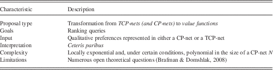
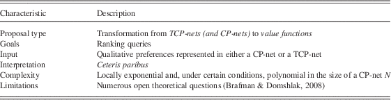
Given that reasoning about preferences represented by value functions is easy as they establish an order among options by ordering computed values, Brafman and Domshlak (Reference Brafman and Domshlak2008) propose an approach for compiling the information captured by CP-nets and TCP-nets into value functions, as described in Table 8. The approach assumes that preference statements have already been elicited from or informed by users, and represented as a TCP-net—or a CP-net, in case there is no (conditional) relative importance between pairs of attributes. The graphical structure plays an important role in analysing and compiling these statements.
Reference card: graphically structured value-function compilation
TCP-nets=Trade-offs-enhanced conditional preference networks; CP-nets=Conditional preference networks.
This work proposes to use a TCP-net to initially organise qualitative preference statements obtained from the user. Then, this information is compiled into a value function that maintains the qualitative structure and independence assumptions implicit in the TCP-net. This obtained value function is used as the model of the user’s ordinal preference and, as new information is received from the user, this value function is refined, while still maintaining the independence assumptions implied by the original TCP-net, if possible.
A TCP-net can be represented as a value function, as it defines a (partial) order among outcomes. The main challenge is to investigate whether there exists a GA value function defined over small factors ‘implied’ by the structure of the network, that is, to find a structured value function that, in some sense, is as compact as the original TCP-net. In order to do so, it is necessary to define a GA value function whose factors are the families of the CP-net. A CP-family is the set that includes a particular attribute and its parents. For instance, considering the example of Section 5.1, the CP-family of S is {S} (as it has no parents), while that of W is {W, S} (W is the attribute and S its parent). Every acyclic CP-net is GA-decomposable over its CP-families; that is, a CP-family is a utility-independent set of attributes. In order to identify the weights of the value function, a system of linear inequalities (CP-conditions) is constructed and solved. The same applies to TCP-nets; that is, every acyclic TCP-net is GA-decomposable over its TCP-families. A TCP-family, in turn, is composed of a particular attribute, its parents, and also the attributes that impose conditionality on the target attribute. For instance, in the example of Section 5.2, the TCP-family of W is {W, S, D} (W is the attribute, S is its parent, and S and D impose conditionality on W).
This value-function compilation is not only efficient and sound, but also complete; that is, the ability to generate the value function is guaranteed. A system of linear inequalities L, either for CP-nets or TCP-nets, is locally exponential. However, if the maximum cardinality of all extended CP-families (an attribute, its parents, its children, and its children’s parents) of a CP-net N is a constant k, a value function consistent with N can be constructed in time polynomial in the size of N. This also holds for TCP-nets.
Because this work relies on TCP-nets (and CP-nets), limitations regarding the representation of preferences and their interpretation are also related to this work. Moreover, the authors themselves point out that their work raises numerous open theoretical questions, including (Brafman & Domshlak, Reference Brafman and Domshlak2008): (i) when (if at all) is GA-decomposition complete for cyclic TCP-nets, or even just cyclic CP-nets and (ii) what is the most compact form of GA-decomposition that is complete for all consistent TCP-nets.
6 Constraint programming
Most of the approaches presented in the previous sections focus on representing preferences as order statements. Another common way of expressing preferences is to use constraints, and constraint solvers can be used to identify optimal options given a set of constraints. Such problems can be formally specified as CSPs, which are mathematical problems defined as sets of objects (options) whose state must satisfy a number of constraints or limitations. Constraints can be seen as preferences that should ideally be satisfied, but when no solution is found for an over-constrained problem, these (soft) constraints can be relaxed. Typically, each constraint is associated with a penalty for not being satisfied (or a degree of preference for its satisfaction), and there is an objective of minimising the penalty (or maximising preference satisfaction). In this section, we present approaches that use CSPs to deal with preferences.
6.1 Semiring-based constraint satisfaction
Different approaches have been proposed as extensions to CSPs to deal with soft constraints, that is, when constraints are used to formalise desired (preferred) properties rather than requirements that cannot be violated (Freuder & Wallace, Reference Freuder and Wallace1992). Examples are the fuzzy (Dubois et al., Reference Dubois, Fargier and Prade1993) and weighted (Schiex et al., Reference Schiex, Fargier and Verfaillie1995) CSPs.
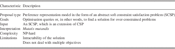
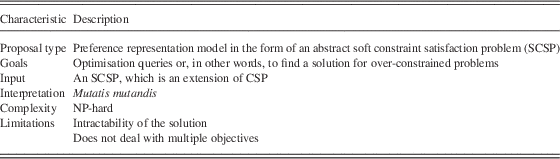
As many extensions to CSPs have been proposed, a constraint solving framework (Bistarelli et al., Reference Bistarelli, Montanari and Rossi1997; Meseguer et al., Reference Meseguer, Rossi and Schiex2006) has been defined (described in Table 9), where all such extensions, as well as classical CSPs, can be cast, namely the soft constraint satisfaction problem (SCSP). The main idea is based on the observation that a semiring—an algebraic structure, with a domain plus two operations satisfying certain properties—is all that is needed to describe many constraint satisfaction schemes.
Reference card: semiring-based constraint satisfaction
CSP=Constraint satisfaction problem.
Semiring-based constraints rely on a simple algebraic structure, called a constraint-semiring or c-semiring (as it is very similar to a semiring), to formalise the notion of satisfaction degrees or preference levels. These establish if a value associated with a constraint is the degree of preference for satisfying the constraint or the penalty for not satisfying it. The structure is specified by a set E of satisfaction degrees, where two binary operators are defined: ×s specifies how to combine preferences, while +s is used to induce a partial ordering on E. Additional axioms, including the usual semiring axioms, are added to precisely capture the notion of satisfaction degrees in soft constraints.
A c-semiring is a 5-tuple 〈E, +s, ×s, 0, 1〉 such that:
∙ E is a set, 0∈E, 1∈E;
∙ +s is an operator closed in E, associative, commutative and idempotent, for which 0 is a neutral element and 1 an annihilator;
∙ ×s is an operator closed in E, associative and commutative, for which 0 is an annihilator and 1 a neutral element; and
∙ ×s distributes over +s.
Compared with a classical semiring structure, the additional properties required by a c-semiring are the idempotency of +s (to capture a lattice ordering) and the existence of a minimum and a maximum element (to capture hard constraints).
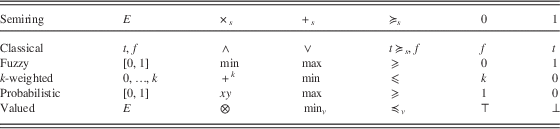
The c-semiring is a generic framework for representing soft constraint problem solvers and, by capturing their commonalities in a generic framework, one can design generic algorithms and properties instead of several apparently unrelated, but actually similar properties, theorems, and algorithms. Examples of different specific frameworks are presented as soft constraint networks (Meseguer et al., Reference Meseguer, Rossi and Schiex2006), which are summarised in Table 10.
Different specific frameworks modelled as c-semirings (Meseguer et al., Reference Meseguer, Rossi and Schiex2006)
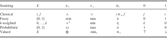
c-semirings=Constraint-semirings.
Given that we now have an algebraic structure to deal with preferences, we must define two other concepts needed to specify a constraint problem—constraint system and constraint—both involving the choice of a c-semiring. Basically, an SCSP defines the c-semiring being used, a set of attributes that describe an application area, and their associated domains. In addition, there is a set of constraints, each associated with a value that is interpreted according to the chosen c-semiring. Formally, an SCSP is defined as follows (Bistarelli et al., Reference Bistarelli, Montanari and Rossi1997).
Constraint system. A constraint system is a tuple CS=〈S, F, X〉, where S is a c-semiring, F a finite set, and X an ordered set of attributes.
Constraint. Given a constraint system CS=〈S, F, X〉, a constraint over CS is a pair 〈def, con〉, where
∙ con⊆X is called the type of the constraint; and
∙ def : F k → A (where k is the cardinality of con and A the set of possible values representing the penalty, cost, preference, weight, etc.) is called the value of the constraint.
Constraint problem. Given a constraint system CS=〈S, F, X〉, a constraint problem P over CS is a pair P=〈C, con〉, where C is a set of constraints over CS and con⊆X. It is also assumed that 〈def 1, con′〉∈C and 〈def 2, con′〉∈C implies def 1=def 2.
In the SCSP framework, the values specified for the tuples of each constraint are used to compute corresponding values for the tuples of values of the attributes in con (set part of the constraint problem), according to the semiring operations: the multiplicative operation is used to combine the values of the tuples of each constraint to get the value of a tuple for all the attributes, and the additive operation is used to obtain the value of the tuples of the attributes in the type of the problem. More precisely, this is the definition of the operations of combination and projection over constraints.
As semiring-based constraints properly generalise classical constraints, this task is NP-hard. As in the classical case, perhaps the most direct way to solve a soft constraint network is searching in its state space, exploring the set of all possible assignments. As an optimal solution is an assignment that minimises the violation degree (or equivalently, maximises the satisfaction degree), optimally solving a soft constraint network is an optimisation problem, and is thus harder than solving classical constraint networks. Different techniques have been proposed to optimise the resolution of this problem, such as defining lower and upper bounds of branch-and-bound algorithms.
Although constraints provide a means of representing qualitative preferences, most of the soft constraint-based approaches also involve the specification of quantitative preferences for each constraint, which is often less intuitive for users. Another limitation of this approach is that it does not deal with multiple objectives; the only objective is to maximise the constraints that are satisfied (considering their weight), but additional objectives such as minimising price cannot be represented. Only intervals for acceptable prices can be provided as constraints.
6.1.1 Extensions
There are extensions of the c-semiring framework, with the goal of representing other kinds of preferences. Next, we briefly describe two of these extensions.
Representing bipolar preferences. Bistarelli et al. (Reference Bistarelli, Pini, Rossi and Venable2010) state that preferences on a set of possible choices are often expressed in two forms: negative and positive statements. The former restricts the set of acceptable options, indicating what users do not want, and the latter indicates options that users prefer with respect to other acceptable options. These two kinds of preferences are referred to as bipolar preferences. The approach described for bipolar preferences (Bistarelli et al., Reference Bistarelli, Pini, Rossi and Venable2010) provides a tool to represent the two types of preference in a single framework and provides algorithms that, given as input a problem with these preferences, return its best solutions.
Representing intervals. Gelain et al. (Reference Gelain, Pini, Rossi, Venable and Wilson2010) argue that it is difficult to specify precise values associated with constraints to represent preferences, and it is more reasonable to consider intervals instead of specific values. They thus developed algorithms to find optimal solutions and also to test whether a solution is optimal based on a set of concepts associated with intervals, such as interval-valued soft constraints and preference intervals.
6.2 Combining conditional preference networks and soft constraints
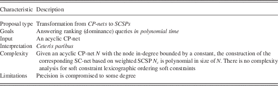
Domshlak et al. (Reference Domshlak, Rossi, Venable and Walsh2003, Reference Domshlak, Prestwich, Rossi, Venable and Walsh2006) establish a connection between CP-nets and soft constraints machinery, with an approach introduced in Table 11. As dominance queries are hard to answer using a CP-net structure (Section 5.1), they propose constructing a semiring structure with a given acyclic CP-net, in order to be able to do so.
Reference card: combining CP-nets and soft constraints
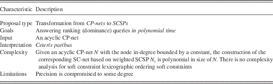
CP-nets=Conditional preference networks; SCSP=Soft constraint satisfaction problem.
This approach thus consists of approximating CP-nets via soft constraints, that is, defining an SCSP based on a CP-net. This provides a uniform framework that combines user preferences with both hard and soft constraints. Thus, given an acyclic CP-net, a corresponding SCSP is constructed in two steps. First, a constraint graph, named SC-net, is built. Second, preferences and weights for the constraints in the SC-net are computed, where this computation depends on the actual c-semiring framework being used. Basically, the SC-net constructed consists of one node for each node of the CP-net plus new nodes for nodes from the CP-net that have more than one parent. Arcs correspond to hard and soft constraints, where the latter are associated with weights and penalties. To calculate these values, two alternative c-semiring frameworks can be used (perhaps other may be used): the min+c-semiring is used for weighted soft constraint satisfaction problems (WSCP), and the S SLO c-semiring is used for soft constraint lexicographic ordering (SLO):
 $${\bf WSCP}:S_{{\min \!\!\plus}}}=\left\langle {R\!_{{\plus}}\!,\min ,\,{\plus}\!,\,{\plus}\!\infty,0} \right\rangle $$
 $${\bf SLO}:S_{{{\rm SLO}}} =\left\langle {A,{\rm max}_{S} ,{\rm min}_{S} ,{\bf MAX},\bf 0} \right\rangle $$
where A is the set of sequences of n integers from 0 to MAX, MAX the sequence of n elements all equal to MAX, and 0 the sequence of n elements all equal to 0; maxS and minS the additive and multiplicative operators, respectively; maxS selects the maximum of two sequences, while minS selects the minimum of two sequences, both considering a lexicographic order.
In both cases, the computation of preferences and weights ensures information preservation and satisfies the CP-condition, that is, approximations preserve the ceteris paribus property.
Precision is compromised to some degree. Different approximations of CP-net ordering via soft constraints (such as min+ and SLO) can be characterised by how much of the original ordering they preserve, the time complexity of generating the approximation, and the time complexity of comparing outcomes in the approximation. Incomparable outcomes with min+ are considered equal or ordered in either way, and with SLO, a strict order will always be defined.
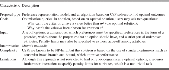
6.3 Preference-based problem solving for constraint programming
Junker (Reference Junker2008) points out that traditional optimisation approaches compile preferences into a single utility function and use it as the optimisation objective when solving the problem, but they do not explain why the resulting solution satisfies the original preferences, and do not indicate the trade-offs made during problem solving. He then argues that the whole problem-solving process becomes more transparent and controllable by the user if it is based on the original preferences.
The problem of multi-objective optimisation was thus tackled by decomposing it into alternative sequences of single-criterion optimisation problems, which can be solved by standard optimisers, with an approach detailed in Table 12. The chosen sequence gives information that explains the optimality of the solution. Based on the explanation, the user can either accept the solution or modify the preferences. The problem solver then modifies the solution correspondingly. Preferences thus allow the user to interact with the problem solver and to control its behaviour.
Preference-based problem solving for constraint programming
CSPs=Constraint satisfaction problems.
This work considers a finite set of attributes X where each attribute x∈X has a domain D(x). The problem space of X is restricted by defining constraints on attributes in X. A constraint c has a scope X c⊆X and a ‘relation’, which is expressed by a set R c of assignments to the scope X c. Such constraints define the set of available options. Consider our example of dinner configurations used to explain TCP-nets, where we have four different attributes: soup (S), wine (W), salad (A), and dessert (D), and each of these attributes has two possible values in its domain. In this scenario, we have 16 possible different configurations, and we can restrict our problem space to the available options, for example, all configurations that serve chocolate as dessert, serve red wine to drink.
Users must provide as input preferences on certain properties of the option. These criteria are mathematical functions from the problem space to an option domain. Formally, a criterion z with domain Ω is an expression f(x 1, … , x n) where x 1, … , x n are attributes from X and f is a function of signature D(x 1)× … ×D(x n)→Ω. Function f can be formulated with the operators of the constraint language (e.g. sum, min, max, conditional expression) or by a table. For example, suppose we are interested in specifying preferences over dishes. A function f may map the dishes to types of dishes, such as light, vegetarian, and so on, so that users may specify their preferences over dish types, and not only over particular attribute values.
Given this, the user can compare different options in a domain Ω and formulate preferences between them. Preferences are modelled in the form of a preorder ≳ on Ω, which consists of a strict part ≻ and an indifference relation ∼. The user may also formulate wishes about the properties that an option should have. Such a wish is a soft constraint which should be satisfied if possible. A wish for constraint c can thus be modelled by a preference 〈z c,>〉, which is abbreviated by wish(c). For example, if the user wants chocolate for dessert (c=D c), then the wish is wish(D c).
As opposed to combinatorial problems with preferences, which are classically solved by compiling all preferences into a single utility function and by determining an option satisfying the constraints with maximal or nearly maximal utility, Junker (Reference Junker2008) uses individual preferences with constraint solvers, in order to allow the optimiser to give an explanation of optimality in terms of the original preferences. First, an atomic optimisation step is performed, which finds options satisfying the constraints C that assign a ≻-maximal value to a single criterion z. This is possible if the user provides a total order over the domain of z, otherwise all possible total orders are generated based on the provided partial order, and the constraint solver runs for each possible total order. Maximal options in this case are the union of maximal options of each of them.
In order to address multiple criteria optimisation, an importance order is introduced on the preferences, also to decide trade-offs in favour of more important preferences. Lexicographic optimisation is then used to define an ordering on the option space based on this importance principle, which leads to finding a lexicographically optimal option. As the importance among the criteria is unknown, permutations of all possible orders are done. If users are not satisfied with the results, they can establish the importance among the criteria, which is a strict partial order I⊆Z×Z, so that only permutations that respect this strict partial order will be considered.
Finally, pareto-optimality is adopted to capture all the possible trade-offs, because using a lexicographic approach gets the best value for a more important criterion z 1, while a less important criterion z 2 is completely penalised, which is a limitation discussed for some of the previously presented approaches. In this case, pareto-optimal options are found, which are those that pareto-dominate other options, that is, optional options are better for at least one criterion, and equally good for the others. As there is no direct way to transform a pareto-optimisation problem into a solved form of the optimisation problem even if it is based on totally ordered preferences, wishes establish penalty limits for criteria.
One of the most challenging problems in preference reasoning is dealing with trade-offs. When a solution is optimal for all criteria, it is trivially optimal. However, requiring users to establish penalty limits for resolving trade-offs has two main drawbacks: (i) for domains that users are not very familiar with, they might only have a vague idea of what is a good limit to establish for the trade-off and (ii) this solution may lead to a situation in which the most important criterion is maximised to a value that sets the maximum penalty to the least important criterion, yet users may prefer something in between. It is important to note that this trade-off resolution involves user interaction.
7 Query-based approaches
Most of the presented approaches were investigated in the context of AI and constraint programming, but more recently preferences have also been taken into account in research related to databases. This is mainly motivated by scenarios resulting from the emergence of the World Wide Web, as users search online store databases and their specified preferences often result in a query being over-constrained, giving no result. In addition, Web search engines provide a huge amount of results for a set of keywords (a query), which can be reduced and ranked if preferences are taken into account. This section presents work that aims at integrating preferences into query languages.
7.1 Winnow
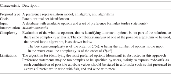
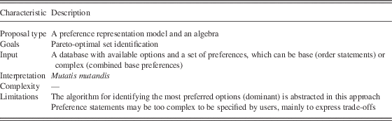
An extension to relational algebra was proposed by Chomicki (Reference Chomicki2003) as a preference query formalisation, in which preferences are expressed as binary relations between tuples from the same database relation; these tuples represent options to be selected. The approach, whose reference card is shown in Table 13, defines a central algebraic operator (winnow), which selects the set of dominant options from a database according to provided preferences. This operator has algebraic properties analysed, such as commutativity, commutation of selection or projection, and distribution of winnow over union and difference. Analysing such properties of winnow is important as they can be exploited for formulating efficient database query execution plans.
Reference card: winnow
In order to identify the pareto-optimal set, this work requires a database with available options and a set of preference formulas. The database is specified in a relation schema R(x 1, … , x n), where each x i is an attribute. Each attribute x i is associated with a domain D i, which is one of two infinite domains: U (uninterpreted constants) and Q (rational numbers). A relation ≻ is a preference relation over R if it is a subset of (D 1× … ×D n)×(D 1× … ×D n). In addition, this preference relation has the following properties: irreflexivity, asymmetry, transitivity, negative transitivity, and connectivity. A preference formulaC(o 1, o 2), on the other hand, is a first-order formula defining a preference relation ≻ in the standard sense, namely o 1 ≻co 2 iff C(o 1, o 2). An intrinsic preference formula (ipf) is a preference formula that uses only built-in predicates.
Because two specific domains are considered, U and Q, there are two kinds of attributes, U-attributes and Q-attributes, and two kinds of atomic formulas: (i) equality constraints and (ii) rational-order constraints. It is assumed that ipfs are in DNF (Disjunctive Normal Form) and quantifier-free. Moreover, atomic formulas are closed under negation. Indifference is also defined: every preference relation ≻c generates an indifference relation ~c: two options o 1 and o 2 are indifferent (o 1 ~co 2) if neither is preferred to the other, that is, o 1 ≻co 2 and o 2 ≻co 1. We show an example of a preference formula below, which expresses ‘I prefer white wine with fish, and red wine with meat’. In this example, d and d′ are dishes, dt and dt′ are dish types, w and w′ are wines, and wt and wt′ are wine types:
 $$\eqalignno{ (d,dt,w,wt)\ {\succ}_{C} (d',dt',w',wt')\,\equiv\,(d=d' & \wedge dt = ‘{\rm fish}’ \wedge wt=‘{\rm white}’ \cr &\! \wedge dt'={\rm ‘ fish} ’ \wedge wt'={\rm ‘red} ’) \cr \vee(d=d' & \wedge dt={\rm ‘ meat} ’ \wedge wt={\rm ‘red} ’ \cr & \wedge dt'=\! {\rm ‘ meat} ’ \wedge wt'={\rm ‘ white} ’ ) $$
Note that in this preference formula any white wine is preferred over any red wine for fish or meat (as there is no w=w′ in the formula), while only equal dishes are compared (because of the d=d′). As d=d′, stating only a value for dt or for dt′ would have been enough.
In order to reason about provided preferences, an algebraic operator called winnow, whose definition is presented below, picks from a given relation the set of the most preferred (dominant) options, according to a given preference formula. A preference query is a relational algebra query containing at least one occurrence of the winnow operator.
Winnow. If R is a relation schema and C a preference formula defining a preference relation ≻ Cover R, then the winnow operator is written as ω C(R), and for every instance r of R:
 $$\omega _{C} (R){\rm =}\{ o\in r\,\mid\,\neg \exists o'\in r.o'{\succ}_{C} o\} $$
There are three possible algorithms (Chomicki, Reference Chomicki2003) to evaluate winnow. The first is a nested-loops algorithm, which compares every two options and discards dominated ones. This algorithm is correct for any preference relation ≻. The second, BNL, is an algorithm proposed by Börzsönyi et al. (Reference Börzsönyi, Kossmann and Stocker2001) in the context of a specific class of preference queries, namely skyline queries, but the algorithm is considerably more general than the previous one. The third (Chomicki et al., Reference Chomicki, Godfrey, Gryz and Liang2005), SFS, is a variant of the second, in which a presorting step is used. The BNL and SFS algorithms require the preference relation to be a strict partial order.
7.2 Best-matches-only query model
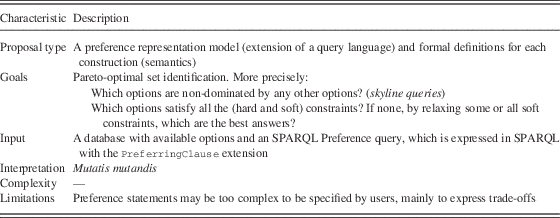
Kießling (Reference Kießling2002) defines preferences as strict partial orders and proposes several preference constructors in order to support the accumulation of single preferences into more complex ones. He also provides a collection of algebraic laws to manipulate such preference constructions, and specifies how to evaluate preference queries under the best-matches-only (BMO) query model (which is very similar to the winnow operator) and decomposition algorithms for complex preference queries. The reference card of his approach is presented in Table 14.
Reference card: best-matches-only query model
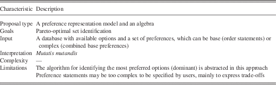
The input needed for querying the pareto-optimal set is a database with available options and a set of preferences. The database specifies a set X of attribute names x i, each associated with a domain D i. A preference P is a strict partial order P=(x i, <P), where <P⊆D i×D i. <P is irreflexive and transitive (which imply asymmetry), and ‘p<P q’ is interpreted as ‘I like p better than q’.
In order to build preferences, many constructors are provided. To build base preferences, there are two classes of constructors: (i) non-numerical base preferences, which include positive and negative preferences, to specify for instance a desired laptop brand and (ii) numerical base preferences, which include preferences that specify preferred numerical values of an attribute using, for example, intervals, such as indicating a desired laptop price range. A preference term (i.e. a preference that is valid according to the provided constructors) can also be composed of other preferences. This can be used to express complex preferences, indicating that two preferences are equally important or that one is more important than another, for example.
The BMO result set contains only the best matches with respect to the strict partial order of a preference P. It is a selection of options that are unordered. All options o, o′∈BMO have equal or incomparable values regarding the preference P. A preference query is defined by σ[P](R) declaratively as follows: σ[P](R)={o∈R|o[x i]∈max(P R)}. σ[P](R) evaluates P against a database set R by retrieving all maximal values from P R. Preference queries behave non-monotonically, in that they are sensitive to the quality of a collection of values. In addition, operators used to specify combined preferences can be manipulated, according to their properties, in order to evaluate preference queries.
7.3 SPARQL Preference
SPARQL Preference (Siberski et al., Reference Siberski, Pan and Thaden2006), introduced in Table 15, is a query language used for querying semantic data. It is based extensively on the winnow operator (Chomicki, Reference Chomicki2003), which was described in Section 7.1.
Reference card: SPARQL Preference
The input of this approach is a database with available options and an SPARQL Preference query, which is expressed in SPARQL with the PreferringClause extension, shown below.
Users can specify preferences that do not overwrite each other, by using the preferring clauses with the definitions of independent preferences separated by the ‘AND’ construct. In each of the preferences connected by the end construct, atomic preferences can be nested using the ‘CASCADE’ construct (which establishes a lexicographic preference among the specified preferences). Atomic preferences can express desired attribute preferences, or indicate that an attribute should be maximised or minimised.
The SPARQL Preference syntax allows the modelling of two kinds of preferences and two kinds of preference interactions, the semantics of which is described informally as follows. For a formal definition, we refer the reader elsewhere (Siberski et al., Reference Siberski, Pan and Thaden2006).
∙ Boolean preferences: boolean preferences are specified by a boolean expression over options (solutions) of an ontology defined in OWL DL (Patel-Schneider et al., Reference Patel-Schneider, Hayes and Horrocks2004). An option o 1 dominates an option o 2, if the boolean expression evaluates to true for o 1, and false for o 2.
∙ Scoring preferences: a scoring preference is specified by an expression, which evaluates to a number or a value in other SPARQL domains that have a total ordering. It expresses the preference for maximising or minimising a certain value. Therefore, an option o 1 dominates o 2, if o 1 has a higher (lower) value than o 2, when a HighestPreference (LowestPreference) is defined.
∙ Multi-dimensional preferences: this kind of preference interaction indicates that two preferences must be addressed in a combined form. For any solutions o 1 and o 2, the domination relation to combine independent preferences
 ${\succ}_{{\,\mid\,C1\,AND\,C2\,\mid\,}} $
establishes that o 1 is dominated by o 2 in neither C1 nor C2, and that o 1 dominates o 2 in either C1 or C2.
∙ Cascaded preference: a cascaded preference indicates that a preference C1 has a higher priority than C2. So, for any options o 1 and o 2, the domination relation to combine prioritised preferences
${\succ}_{{\,\mid\,C1\,CASCADE\,C2\,\mid\,}} $
states that either o 1 dominates o 2 according to C1, or they are incomparable according to C1, and o 1 dominates o 2 according to C2.


An example of a SPARQL query is shown below, in which hotels are being searched using an ontology whose prefix is ht. The query specifies a hard constraint (FILTER (?stars=pt : two || ?stars=pt:three)), which states that only hotels with two or three stars should be selected. The PREFERRING clause states that: (i) 3-star hotels are preferred and (ii) hotels whose check-in time is before 14:00, and from these, those with the lowest price are preferred.
SELECT ?hotel
WHERE {?hotel ht:has-stars ?stars .
?hotel ht : checkin ?checkin .
?hotel ht : price ?price.
FILTER (?stars=ht : two || ?stars=ht:three)}
PREFERRING
?stars=pt : three
AND
?checkin <= 14:00 CASCADE LOWEST(?price)
Based on the definition of dominance among options, a SPARQL Preference query returns as result all non-dominated options (skyline queries). If an option o 1 dominates o 2 according to a preference C1, but o 2 dominates o 1 according to a preference C2, both options are presented as the result of the query.
The major problem of this approach, and of the other query-based approaches, occurs when the best options are not found, according to the stated preferences, which is a typical situation, because trade-off among conflicting preferences is very common. For instance, consider a user that wants to buy a laptop and prefers to minimise price and maximise performance. The typical case here is that price increases as performance increases and, therefore, according to these preferences no laptop dominates another (there is none, or only a few laptops, that are more expensive and have worse performance), and consequently the approach cannot select among these laptops.
8 Discussion
In this section, we provide a comparison of the presented approaches. As stated in the introduction, our goal is not to rate these approaches in order to choose the best, but to better understand them and their relationships. We start by summarising the key characteristics of the approaches to reasoning about preferences, which are depicted in Table 16. For each approach, we show six different aspects, presented in the respective columns.
∙ Area: indicates to which research area the approach is mainly related.
∙ Proposal type: the proposal types shown in the table follow the classification introduced in Section 2. The acronyms used are as follows: PRM—Preference Representation Model; ALGO—Algorithms; ALGE—Algebra; SEM—Semantics; TRANS—Transformation.
∙ Goals: the goals shown in the table follow the classification introduced in Section 2. The acronyms used are as follows: OPQ—optimisation queries; RNK—ranking queries; POS—pareto-optimal set identification.
∙ Preferences: provides a general classification for the preferences required as an input of the approach.
∙ Reasoning: classifies the reasoning method adopted by the approach as quantitative or qualitativeFootnote 1. This paper focuses on approaches that reason about qualitative preferences. Some approaches manipulate such preferences qualitatively, and others transform them into quantitative preferences.
∙ Interpretation: indicates how preference statements are interpreted by the approach. There are three possible options: (i) CP (ceteris paribus); (ii) MM (mutatis mutandis); and (iii) MU (marginal utility)—which is the case of the approach that learns utility functions with SVM.
Comparison among approaches to reason about preferences
SVM=Support vector machine; CP-nets=Conditional preference networks; TCP-nets=Trade-offs-enhanced conditional preference networks; BMO=Best matches only; AI=Artificial intelligence; SCSP=Soft constraint satisfaction problem; CP=Ceteris paribus; MM=Mutatis mutandis; MU=Marginal utility.
By analysing these approaches, we can observe that they address three main problems. First, given a representation of qualitative statements, how can the typical questions (optimisation, ranking, and pareto-optimal queries) related to reasoning about preferences be answered? Second, given a representation of qualitative statements, how can it be transformed into a utility function? Third, how can we represent compact utility functions? In the first problem, preferences are considered easier to elicit than in quantitative approaches, as qualitative statements are considered closer to the user vocabulary, but are difficult to be reasoned about. The third problem is related to approaches that rely on utility functions to reason about preferences, with which one can easily compare options. However, eliciting utility functions is not a trivial task, and for particular contexts, combinations of attribute values have utility values that cannot be represented in a compact form, such as when assuming utility independence among attributes. Therefore, solutions to the second problem aim at obtaining the main benefits of solutions to the first (easy representation) and the third problems (easy reasoning), but the challenge now is the translation of qualitative to quantitative statements. In addition, considering all possible combinations of attribute values is a combinatorial problem, so it is very important to take into account the complexity of reasoning about preferences. We do not discuss complexity in this section, as the worst case takes exponential time to be computed for almost all approaches, while some of these approaches do not have their complexity analysed.
The issue of allowing expression of compact preferences is not only associated with utility functions, but also with approaches that are able to deal only with boolean values. Although multi-valued attributes can be translated into boolean attributes—for example, the attribute colour with values red and yellow can be translated to two boolean attributes colour_red and colour_yellow, and these attributes are mutually exclusive—expressing consistent preferences over boolean attributes may require more verbose preference statements. For example, a simple statement red≻yellow should be  $$(colour\_red\wedge\neg colour\_yellow)\,{\succ}\,(colour\_yellow\wedge\neg colour\_red)$$
. This additional effort can be reduced by pre-processing and automatically translating preference statements given by users; however, as multi-valued attributes may have many possible values and each value becomes an attribute, if an approach that represents only boolean values is used, this may compromise the performance of the approach, because the complexity of most approaches depends on the number of attributes.
All the approaches aim to help users to make decisions of choosing from among alternatives, but based on the investigated approaches we can classify this into two categories: (a) helping users to make decisions in situations in which it is hard for them to compare options and identify the best one due to uncertainty or trade-off among options and (b) helping users to make decisions in situations in which they would be able to make a choice but, due to the large number of the options, it is practicably infeasible for the users to analyse all options. Even though, in the end, the problem to be solved is the same in these two categories, they differ in a very relevant aspect: engagement of users in providing information about their preferences. A typical scenario for (a) is a company manager that must decide on an action to be taken, where this action has a crucial impact on the profit of the company. In addition, many attributes with uncertain values are associated with this action. Therefore, the manager is willing to spend a significant amount of time to precisely specify preferences among options and related attributes. A typical scenario for (b) is Web users that search with keywords and receive in return a large number of results, which they must filter and rank.
MAUT has the goal described in (a), that is, helping a decision maker to evaluate complex options when their outcomes are uncertain and have several relevant attributes. Therefore, adopting utility functions to represent preferences is reasonable (but still difficult), as users are willing to spend time in eliciting them, that is, when the consequences of making a wrong decision compensate for the time and effort spent in eliciting (and building new) preferences. Even though there is work (McGeachie & Doyle, Reference McGeachie and Doyle2004; Domshlak & Joachims, Reference Domshlak and Joachims2007) that obtains utility functions from qualitative statements, it still has limitations reported in the approaches presented in this paper.
Query-based approaches address the scenario described in (b), and their aim is not to totally automate the decision-making process, but to provide reduced number of results to users, possibly ranked. Considering preferences in queries allows users to be more restrictive when providing constraints for queries and still obtain results that contain useful information—if the query is over-constrained it is likely that it will return no results. Therefore, this family of approaches discards dominated options from the results, which are those that have at least one attribute value that is worse than the attribute value of another option, and they are at most as good as for the remaining attributes. Choosing among non-dominated options is a task that is still left for the user, but some heuristics, such as considering lexicographic preference among attributes, can be used to rank them, and give guidance to users.
In order to deal with over-constrained problems, CSPs have been extended to incorporate constraints that can remain unsatisfied, with a non-satisfaction penalty associated with them. These approaches have the objective to minimise the penalty of unsatisfied constraints (or maximising preferences), and other objectives, for example, minimise price, cannot be specified. In addition, trade-off situations among conflicting objectives cannot be modelled, and thus received limited attention (Bistarelli et al., Reference Bistarelli, Gadducci, Larrosa and Rollon2008). Therefore, SCSPs are effective in solving specific classes of problems, for example, meeting scheduling problems.
Last, there are the graphically structured approaches, which structure qualitative preference statements in a graph and adopt the ceteris paribus interpretation. For graphs with certain properties, these approaches can be used efficiently to identify optimal options and, with the proposed techniques (Domshlak et al., Reference Domshlak, Rossi, Venable and Walsh2003), can also answer dominance queries efficiently. However, two options can be compared only when ‘all else is equal’, and in practice this is often not the case. When other attribute values differ, options are considered incomparable and no decision can be made regarding dominance. Moreover, these approaches can deal only with discrete attribute domains, and this is also a very restrictive assumption. Furthermore, trade-off is only captured in TCP-nets, but a lexicographic approach is adopted, unless a fully specified CIT is provided.
All these introduced approaches are relevant in the context of qualitative preference reasoning. In order to illustrate their importance, we introduce research that builds on them in Table 17. For each approach presented in this paper, we selected one piece of work that either extends it, or uses (part of) it for a particular purpose—rather than merely discuss it as related work. As can be seen in Table 17, we present only academic research, as few approaches concern application development. This provides evidence of a deficiency of work on qualitative preference reasoning: few real applications have been developed. Moreover, we are not aware of their adoption by industry. Consequently, developing applications and showing that they can be employed in real-world scenarios is crucial to demonstrate the usefulness of qualitative preference reasoning outside the boundaries of academia.
Example of applications and extensions of the approaches
SVM=Support vector machine; CP-nets=Conditional preference networks; TCP-nets=Trade-offs-enhanced conditional preference networks; CSP=Constraint satisfaction problem.
9 Final considerations
In this paper, we have presented a review of research that aims at helping decision makers to make choices (and even automating this), taking into account their preferences expressed in a qualitative way. We selected approaches that propose different techniques and algorithms, which take as input qualitative multi-attribute preference statements following a particular structure imposed by the approach. Our review was not limited to a specific research area, and included approaches in the context of decision theory, AI, constraint programming, databases, and the Semantic Web. Each of these approaches was presented in the context of an evaluation framework, which facilitates their comparison. Importantly, our review provides an understanding not only of each individual research effort but also, with our discussion, the way in which they are related, the kinds of issues they typically address and their limitations.
This study has shown that a key issue related to reasoning about preferences is dealing with trade-off situations. Both utility functions and (conditional) qualitative statements can capture them, but it is difficult to express these kinds of preferences in a compact form. For instance, if there is no utility independence among attributes, each possible option has a particular utility that cannot be derived from individual attribute values. In the case of qualitative statements, each full assignment for attributes must be compared. Moreover, users typically do not provide these kinds of preferences, because they are constructed only when users face a concrete decision-making situation (Lichtenstein & Slovic, Reference Lichtenstein and Slovic2006).
Acknowledgement
The authors would like to thank the anonymous reviewers for their valuable comments and suggestions to improve this paper. FAPERGS and CNPq #442582/2014-5 are also acknowledged.