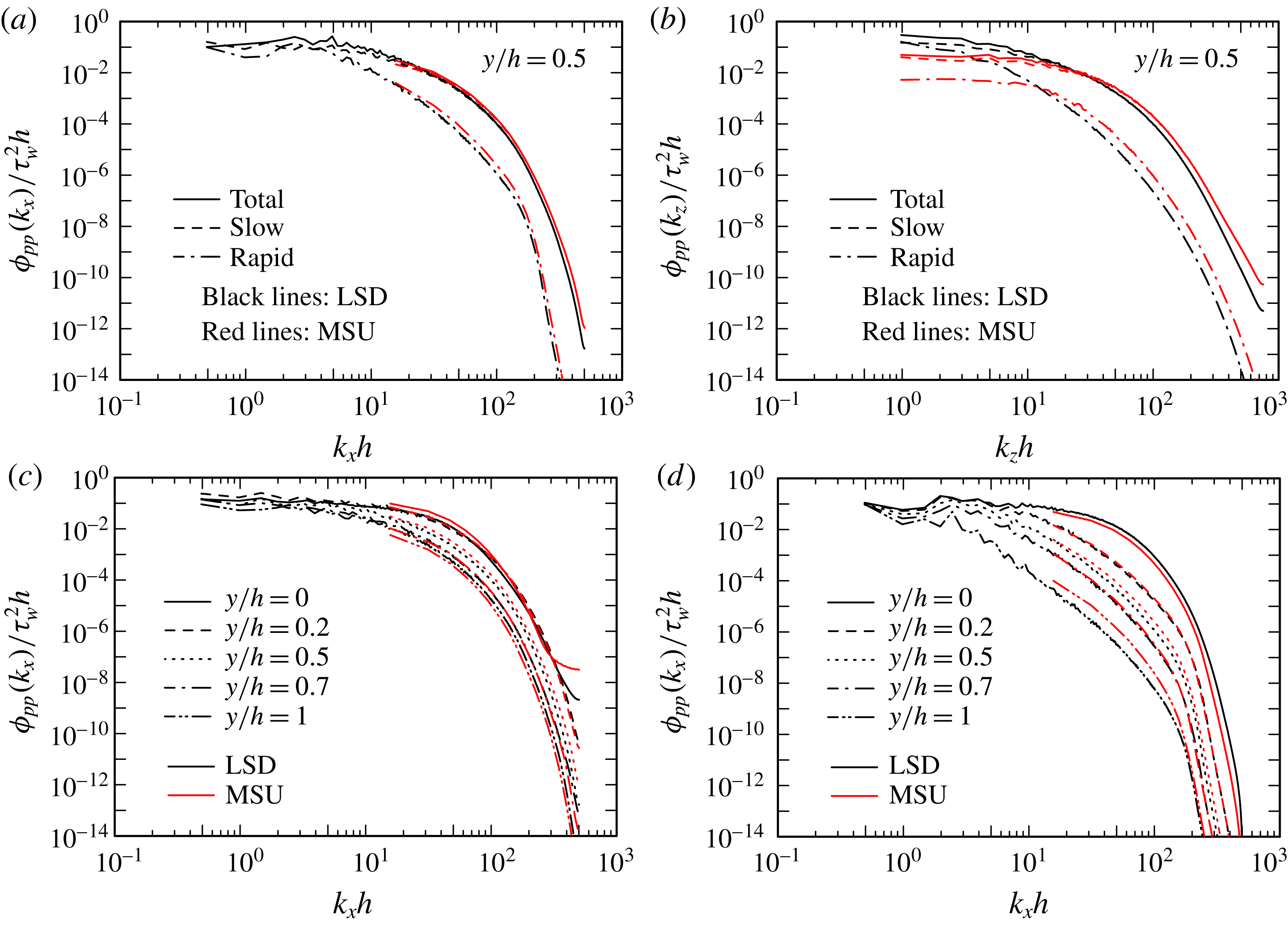
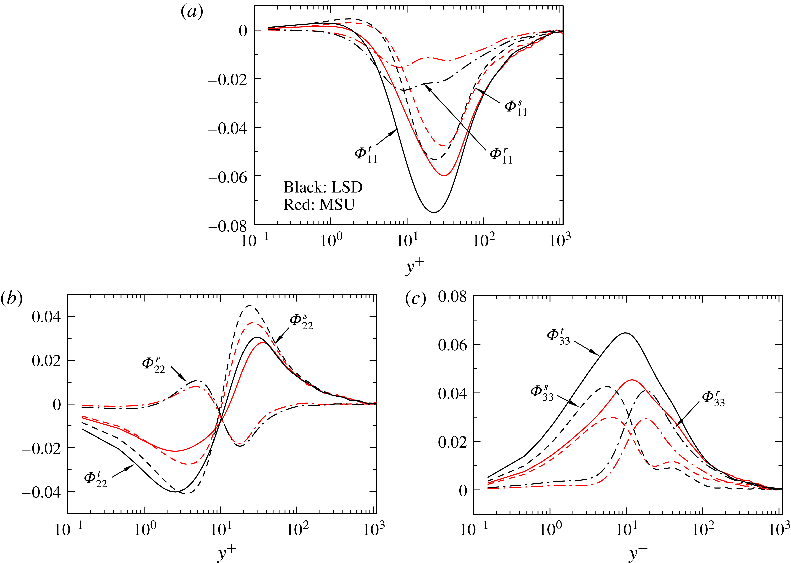
1 Introduction
The structure of a turbulent boundary layer has attracted significant attention over the past several decades. Streaks and quasi-streamwise vortices are intrinsic elements of the organization near a wall (e.g. Kline et al.
Reference Kline, Reynolds, Schraub and Runstadler1967; Robinson Reference Robinson1991), whereas the logarithmic and outer regions are characterized by large-scale motions (LSMs) inclined at
 $12^{\circ }$
–
 $30^{\circ }$
to the wall (e.g. Brown & Thomas Reference Brown and Thomas1977; Rajagopalan & Antonia Reference Rajagopalan and Antonia1979; Christensen & Adrian Reference Christensen and Adrian2001) and their streamwise elongated structures, i.e. very large-scale motions (VLSMs) (e.g. Kim & Adrian Reference Kim and Adrian1999; Balakumar & Adrian Reference Balakumar and Adrian2007; Monty et al.
Reference Monty, Stewart, Williams and Chong2007; Lee & Sung Reference Lee and Sung2011) or superstructures (Hutchins & Marusic Reference Hutchins and Marusic2007a
,Reference Hutchins and Marusic
b
).
Direct numerical simulations (DNSs) have been increasingly used to examine the organized motions in wall turbulence. In a turbulent channel flow, the seminal DNS was made by Kim, Moin & Moser (Reference Kim, Moin and Moser1987) for a Kármán number
 $h^{+}~(\equiv U_{\unicode[STIX]{x1D70F}}h/\unicode[STIX]{x1D708})=180$
. Here,
 $h^{+}$
represents the ratio of the half-width of the channel
 $h$
and the viscous length scale
 $\unicode[STIX]{x1D708}/U_{\unicode[STIX]{x1D70F}}$
(
 $U_{\unicode[STIX]{x1D70F}}(\equiv (\unicode[STIX]{x1D70F}_{w}/\unicode[STIX]{x1D70C})^{1/2})$
is the friction velocity, where
 $\unicode[STIX]{x1D70F}_{w}$
is the wall shear stress and
 $\unicode[STIX]{x1D70C}$
is the density of the fluid; the superscript
 $+$
denotes normalization by wall units). At low to moderate
 $h^{+}$
(
 ${\approx}600$
), a small domain which contains a minimal set of structures that are necessary to sustain a turbulent boundary layer, viz. a minimal flow unit (Jiménez & Moin Reference Jiménez and Moin1991), has been successful for investigating near-wall dynamical behaviours (Jiménez & Pinelli Reference Jiménez and Pinelli1999) (see also Jiménez & Kawahara Reference Jiménez, Kawahara, Davidson, Kaneda and Sreenivasan2011), in particular, for identifying a self-sustaining process (SSP) near a wall (Hamilton, Kim & Waleffe Reference Hamilton, Kim and Waleffe1995; Waleffe Reference Waleffe1997). This simplified flow unit consists of a small box (i.e.
 ${L_{x}}^{+}=400$
and
 ${L_{z}}^{+}=100$
), in which one pair of near-wall streaks and one quasi-streamwise vortex are marginally accommodated (
 $x$
,
 $y$
,
 $z$
denote streamwise, wall-normal and spanwise directions, respectively;
 $x_{1}$
,
 $x_{2}$
,
 $x_{3}$
are also used interchangeably with
 $x$
,
 $y$
,
 $z$
throughout the paper). On the other hand, as
 $h^{+}$
has increased, more attention has been given to organization in the logarithmic and outer regions (viz. LSMs or VLSMs and vortex clusters) with large domains. del Álamo & Jiménez (Reference del Álamo and Jiménez2003) reported two different modes of large-scale
 $u$
structures in the spectra (
 $u$
,
 $v$
,
 $w$
denote the streamwise, wall-normal and spanwise velocity fluctuations, respectively;
 $u_{1}$
,
 $u_{2}$
,
 $u_{3}$
are also used interchangeably with
 $u$
,
 $v$
,
 $w$
; a capital letter is an instantaneous quantity). One is a global mode with a streamwise extent greater than 5
 $h$
and a spanwise extent being approximately 2
 $h$
; its effect penetrates into the wall region (see also the near-wall footprint reported by Abe, Kawamura & Choi Reference Abe, Kawamura and Choi2004b
and Hutchins & Marusic Reference Hutchins and Marusic2007a
and the top–down mechanism described by Hunt & Morrison Reference Hunt and Morrison2001). In this context, del Álamo et al. (Reference del Álamo, Jiménez, Zandonade and Moser2004) also found that the spectral widths of the largest
 $u$
scales are proportional to the square root of their lengths. The other is a quasi-isotropic mode with a streamwise length of 2
 $h$
and a spanwise width equal to
 $h$
. del Álamo et al. (Reference del Álamo, Jiménez, Zandonade and Moser2004, Reference del Álamo, Jiménez, Zandonade and Moser2006) demonstrated that large-scale negative
 $u$
structures are wakes left behind vortex clusters. This bottom-up concept is identical with the hairpin packet paradigm proposed by Adrian, Meinhart & Tomkins (Reference Adrian, Meinhart and Tomkins2000). Jiménez & Hoyas (Reference Jiménez and Hoyas2008) subsequently made a detailed analysis on the two-dimensional energy spectra above the buffer region for very large streamwise domains (VLSDs) up to
 $h^{+}=2000$
. They noted that the longest and widest modes for the
 $u$
spectra (i.e.
 $\unicode[STIX]{x1D706}_{x}/h>5\sim 6h$
and
 $\unicode[STIX]{x1D706}_{z}/h>1\sim 2h$
) are approximately independent of the wall distance (
 $\unicode[STIX]{x1D706}_{x}$
and
 $\unicode[STIX]{x1D706}_{z}$
denote the streamwise and spanwise wavelengths, respectively) and contain energy across the whole flow. The latter modes correspond to the VLSMs and are intrinsically associated with the long conical structures (del Álamo et al.
Reference del Álamo, Jiménez, Zandonade and Moser2004, Reference del Álamo, Jiménez, Zandonade and Moser2006) which are somewhat similar to the inactive attached eddies proposed by Townsend (Reference Townsend1976). Recently, Bernardini, Pirozzoli & Orlandi (Reference Bernardini, Pirozzoli and Orlandi2014) performed DNSs up to
 $h^{+}=4088$
. They noted that the global
 $u$
mode becomes prominent as
 $h^{+}$
increases, most probably due to the advection of the outer modes in a transient growth mechanism (del Álamo & Jiménez Reference del Álamo and Jiménez2006).
While large domains are required for incorporating large-scale motions as accurately as possible, the simplification of the flow field by selecting a flow unit which contains essential elements of large-scale motions may be useful for providing further insight into the outer-layer structures. In this context, Flores & Jiménez (Reference Flores and Jiménez2010) examined a minimal flow unit in the logarithmic and outer regions for
 $h^{+}\approx 1900$
. They noted that a segment containing several streamwise velocity streaks and a vortex cluster, with dimensions of about 6
 $h$
and 3
 $h$
in the
 $x$
and
 $z$
directions, respectively, represents a minimal unit in the logarithmic region, while a smaller domain degrades the magnitudes of
 $v$
and
 $w$
away from the wall. Lozano-Durán & Jiménez (Reference Lozano-Durán and Jiménez2014) further examined effects of both
 $L_{x}$
and
 $L_{z}$
up to
 $h^{+}=4000$
. They reported that correct one-point statistics are obtained when
 $L_{x}\geqslant 2\unicode[STIX]{x03C0}h$
and
 $L_{z}\geqslant \unicode[STIX]{x03C0}h$
.
A different approach has also been taken by Toh & Itano (Reference Toh and Itano2005) who have used a minimal ‘streamwise’ unit (MSU) by assuming that large-scale motions are essentially two-dimensional and infinitely long structures. The MSU consists of a relatively small subspace of a large
 $L_{x}$
domain where not only near-wall structures but also large-scale ones develop spatially and interact with each other. In this system, near-wall and outer large-scale structures are prevented from evolving spatially in the
 $x$
direction, but can evolve in the
 $y$
and
 $z$
directions (i.e. in the cross-stream plane); the focus is thus on the temporal evolution rather than on the spatial evolution. Toh & Itano (Reference Toh and Itano2005) successfully observed a close relationship between near-wall streaks and the large-scale structures (this is referred to as a ‘co-supporting cycle’ in their paper), although their Reynolds number was limited to relatively small values of
 $h^{+}$
(
 $h^{+}=137$
and 349). In their simulation, there is a collective motion of near-wall streaks, which is coupled directly to the LSMs. The flow is also characterized by a large-scale recirculation across the whole channel. The latter behaviour may be inferred from the SSP (Hamilton et al.
Reference Hamilton, Kim and Waleffe1995; Waleffe Reference Waleffe1997) where streamwise rolls having wall-normal and spanwise velocities are intrinsic elements; the latter are decoupled from the streamwise velocity and redistribute the streamwise momentum to create streamwise
 $u$
fluctuations (i.e. streaks). Hwang et al. (Reference Hwang, Lee, Sung and Zaki2016) convincingly identified a collective migration of near-wall streaks in a VLSD at
 $h^{+}=930$
, which is induced by large-scale circulations during the merging of outer long streaks.
Abe et al. (Reference Abe, Kawamura, Toh, Itano, Palma and Lopes2007) performed DNSs for various values of
 $L_{x}$
, down to the size associated with the MSU (viz.
 ${L_{x}}^{+}\approx 400$
) for
 $h^{+}=1020$
. The effect of varying
 $L_{x}$
is important for clarifying not only the role of the streamwise evolution of near-wall and large-scale structures but also the extent to which the interaction between these structures can be described meaningfully in the MSU. It was shown that the inner and outer spanwise organization of
 $u$
does not change appreciably when
 $L_{x}$
decreases whereas the magnitudes of
 $v$
and
 $w$
decrease. It was also found that the pressure redistribution is weakened when
 $L_{x}<2\unicode[STIX]{x03C0}h$
since the turbulent kinetic energy is not redistributed properly to
 $\overline{v^{+}v^{+}}$
and
 $\overline{w^{+}w^{+}}$
(an overbar denotes averaging in both space and time) (see Abe & Antonia Reference Abe and Antonia2016). In particular, the rate of decrease, with decreasing
 $L_{x}$
, of the streamwise and spanwise pressure strain terms
 $\unicode[STIX]{x1D719}_{11}^{+}$
and
 $\unicode[STIX]{x1D719}_{33}^{+}$
(defined in § 3.2), is large, which makes
 $\overline{u^{+}u^{+}}$
and
 $\overline{w^{+}w^{+}}$
more and less energetic. The inactive motion (i.e. the large-scale motions and the irrotational pressure fluctuations of the outer region (Townsend Reference Townsend1961; Bradshaw Reference Bradshaw1967)) is thus affected more significantly by
 $L_{x}$
than the active motion. There has not yet been a quantitative assessment of how the MSU behaves as
 $h^{+}$
increases and of how a large
 $L_{x}$
domain differs from the MSU. For the SSP, Waleffe & Kim (Reference Waleffe, Kim and Panton1997) estimated that streamwise rolls (i.e.
 $V$
and
 $W$
) exhibit a 1/Re dependence, whereas streaks (i.e.
 $u$
) remain essentially Re independent. It is however not evident whether or not the large-scale recirculation is present in the MSU at large Reynolds numbers.
In the present study, we extend the scope of the work of Toh & Itano (Reference Toh and Itano2005) to larger
 $h^{+}$
with the use of DNS datasets in a turbulent channel flow. The streamwise extent of the MSU (
 ${L_{x}}^{+}\approx 400$
) is identical to that of Toh & Itano (Reference Toh and Itano2005), but the spanwise dimension
 $L_{z}$
is larger (
 $L_{z}=6.4h$
, compared to
 $L_{z}=2.4h$
for Toh & Itano Reference Toh and Itano2005 at
 $h^{+}=349$
) in order to retain the influence of the spanwise stripe patterns associated with both near-wall and outer-layer structures. Two Kármán numbers,
 $h^{+}=395$
and 1020, are used. The latter value is sometimes used as a lower limit for which the inner and outer regions are distinguishable (see Monty & Chong Reference Monty and Chong2009) so that datasets with significantly different streamwise domains (
 $L_{x}=0.4h$
to
 $12.8h$
) can allow us to examine the dependence of the streamwise inclination of the LSMs on
 $L_{x}$
. The streamwise inclination of the LSMs is of importance in the contexts of the spatial growth of structures and the interaction between structures aligned in the streamwise direction (see Adrian et al.
Reference Adrian, Meinhart and Tomkins2000; del Álamo et al.
Reference del Álamo, Jiménez, Zandonade and Moser2006). The upper bound of the logarithmic region is
 $y/\unicode[STIX]{x1D6FF}=0.15$
(
 $\unicode[STIX]{x1D6FF}$
denotes the boundary layer thickness) in a boundary layer (Hutchins & Marusic Reference Hutchins and Marusic2007a
), although
 $y/h=0.2$
has sometimes been identified as the upper bound of the logarithmic region in a channel flow (e.g. Jiménez & Hoyas Reference Jiménez and Hoyas2008). In this paper, we compare the present DNS data for the MSU with those for a large streamwise domain (denoted hereafter by LSD), where
 $L_{x}=12.8h$
, for
 $h^{+}=180$
to 1020 and also with other DNS data in the literature (del Álamo et al.
Reference del Álamo, Jiménez, Zandonade and Moser2004; Hoyas & Jiménez Reference Hoyas and Jiménez2008; Bernardini et al.
Reference Bernardini, Pirozzoli and Orlandi2014; Lee & Moser Reference Lee and Moser2015) with VLSDs of streamwise extent
 $L_{x}=6\unicode[STIX]{x03C0}h\sim 8\unicode[STIX]{x03C0}h$
and
 $h^{+}$
extending up to 5000. A comparison is also made with the experimental data by Wei & Willmarth (Reference Wei and Willmarth1989) for
 $h^{+}=1016$
, Balakumar & Adrian (Reference Balakumar and Adrian2007) for
 $h^{+}=960$
and Monty & Chong (Reference Monty and Chong2009) for
 $h^{+}=1040$
. When
 $L_{x}$
is reduced to the size of the MSU at large
 $h^{+}$
, we expect the large-scale structures in the outer region to become approximately two-dimensional since the streamwise extent of the MSU becomes increasingly smaller in terms of
 $L_{x}/h$
as
 $h^{+}$
increases. One also expects this two-dimensionality to result in an attenuation of the large-scale spanwise meandering due to the continuity constraint (see § 3) given that the wall-normal velocity is not affected by the large-scale inactive motion (Townsend Reference Townsend1976). At large
 $h^{+}$
, the large-scale structures in the MSU are thus expected to lack two features observed in the LSD/VLSD, namely the streamwise inclination and spanwise meandering of the large-scale structures. On the other hand, the spanwise domain for the MSU is sufficiently large to accommodate the spanwise organization of outer-layer structures. While the large-scale structures in the MSU may be considered to be ‘artefacts’ arising from the small value of
 $L_{x}$
, the present work falls in the category of ‘numerical experiments’ (e.g. Moin & Mahesh Reference Moin and Mahesh1998) whose objective is to study in some detail the influence of isolated physical parameters. The main aim of the present study is to establish if the spanwise organization of the large-scale structures (a feature missing in the original minimal flow unit introduced by Jiménez & Moin Reference Jiménez and Moin1991) is sufficiently well captured in the MSU at a value of
 $h^{+}$
as large as 1020; a positive outcome would strengthen Toh & Itano’s (Reference Toh and Itano2005) conclusions regarding the interaction between near-wall and outer large-scale structures in the context of the near-wall turbulence dynamics. We also discuss how the outer large-scale structures in the MSU are associated with the mean streamwise velocity, keeping in mind that the large-scale structures in the LSD/VLSD are active in the context of momentum transport in the present flow (e.g. del Álamo et al.
Reference del Álamo, Jiménez, Zandonade and Moser2004, Reference del Álamo, Jiménez, Zandonade and Moser2006; Balakumar & Adrian Reference Balakumar and Adrian2007). Our focus is to correctly capture the spanwise organization of large-scale structures in the log region whilst making sure that the mean spanwise spacing between these structures is meaningful. The comparison between results obtained for the MSU and LSD/VSLD also allows us to infer, albeit indirectly, the importance of the streamwise inclination and spanwise meandering of the large-scale structures; these features are present in the LSD/VSLD but absent in the MSU. We also note that the reason we use a short domain length (
 ${L_{x}}^{+}=400$
) is to continue to exploit the advantages of the minimal flow unit ‘numerical experiment’ (Jiménez & Moin Reference Jiménez and Moin1991).
The paper is organized as follows. Section 2 describes the present DNS datasets. Section 3.1 discusses the Reynolds-number dependence of basic statistics in the MSU. In § 3.2, we then examine the effect of varying
 $L_{x}$
for
 $h^{+}=1020$
on turbulence statistics and structures. We also discuss the similarity between
 $\overline{ww}$
and
 $\overline{pp}$
(the mean square value of pressure fluctuation) in light of the attached eddy hypothesis (Townsend Reference Townsend1976), and also the relationship between
 $\overline{pp}$
and the energy dissipation rate
 $\overline{\unicode[STIX]{x1D700}}$
(defined in § 3.2). To our knowledge, the latter relationship has not been considered previously. Section 3.3 examines the degree of similarity in velocity fluctuations between the smallest and largest streamwise domains (viz.
 $L_{x}=0.4h$
and
 $12.8h$
) for
 $h^{+}=1020$
. Particular attention is given to hierarchical spanwise
 $u$
organization and the temporal evolution in the MSU where the two-dimensionality of the large-scale structures is established approximately so that both the streamwise inclination and spanwise meandering are inhibited. In § 3.4, we also investigate the pressure fluctuations for the MSU with a focus on the linear and nonlinear interactions (i.e. the rapid and slow pressure).
2 DNS datasets
The present datasets have been obtained from DNSs in a turbulent channel flow with a large
 $L_{x}$
by Abe, Kawamura & Matsuo (Reference Abe, Kawamura and Matsuo2004a
) and Abe, Antonia & Kawamura (Reference Abe, Antonia and Kawamura2009) and with smaller streamwise domains by Abe et al. (Reference Abe, Kawamura, Toh, Itano, Palma and Lopes2007). The flow is a fully developed turbulent channel flow driven by a constant streamwise mean pressure gradient. Two Kármán numbers (
 $h^{+}=395$
and 1020) are used for the MSU (
 ${L_{x}}^{+}\approx 400$
), while four Kármán numbers (
 $h^{+}=180$
, 395, 640 and 1020) are used for the LSD (
 $L_{x}=12.8h$
).
The numerical methodology for the current DNS is briefly as follows. A fractional step method is used with semi-implicit time advancement. The third-order Runge–Kutta method is used for the viscous terms in the
 $y$
direction and the Crank–Nicolson method is used for the other terms. A finite difference method is adopted for the spatial discretization. A fourth-order central scheme (Morinishi et al.
Reference Morinishi, Lund, Vasilyev and Moin1998) is used in the
 $x$
and
 $z$
directions, whilst a second-order central scheme is used in the
 $y$
direction. The periodic boundary condition is employed in the
 $x$
and
 $z$
directions, whereas the no-slip condition applies in the
 $y$
direction. Further details on the simulations are given in Abe, Kawamura & Matsuo (Reference Abe, Kawamura and Matsuo2001), Abe et al. (Reference Abe, Kawamura and Matsuo2004a
,Reference Abe, Kawamura and Choi
b
, Reference Abe, Antonia and Kawamura2009) and Antonia, Abe & Kawamura (Reference Antonia, Abe and Kawamura2009), and the reader may refer to these papers for information on basic turbulence statistics obtained with a large domain.
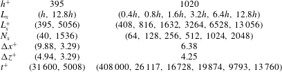
The computational domain size (
 $L_{x}\times L_{y}\times L_{z}$
), number of grid points (
 $N_{x}\times N_{y}\times N_{z}$
) and spatial resolution (
 $\unicode[STIX]{x0394}x$
,
 $\unicode[STIX]{x0394}y$
,
 $\unicode[STIX]{x0394}z$
) for small and large streamwise domains are given in tables 1 and 2, respectively, the superscript
 $^{\ast }$
representing normalization by either
 $v_{K}$
(
 $\equiv (\unicode[STIX]{x1D708}\overline{\unicode[STIX]{x1D700}})^{1/4}$
; the Kolmogorov velocity scale) or
 $\unicode[STIX]{x1D702}$
(
 $\equiv (\unicode[STIX]{x1D708}^{3}/\overline{\unicode[STIX]{x1D700}})^{1/4}$
; the Kolmogorov length scale); the subscripts
 $w$
and
 $c$
refer to the wall and centreline, respectively (note that
 $\overline{\unicode[STIX]{x1D700}}$
denotes the energy dissipation rate, defined in (3.8)). For a large domain, the effect of the domain size was examined by Abe et al. (Reference Abe, Kawamura and Choi2004b
) (
 $h^{+}=640$
) who compared two cases:
 $(L_{x}\times L_{z})=(6.4h\times 2h)$
and (
 $12.8h\times 6.4h$
). They found that the effect on the mean flow variables and second-order moments was negligible. They also examined one-dimensional energy spectra and noted that their streamwise domain size was not large enough to include all the large-scale contributions, whereas their spanwise domain size was quite sufficient. For small domains, it will be shown in § 3.2 that longer scales than
 $L_{x}$
are represented by the infinitely long mode (viz. the zero mode of the energy spectra) and the streamwise inclination of large-scale motions is reduced as
 $L_{x}$
decreases. The smallest domain (
 ${L_{x}}^{+}\approx 400$
) is identical with that in the minimal flow unit in the buffer region (Jiménez & Moin Reference Jiménez and Moin1991).
Domain size, grid points and spatial resolution for the DNS with the varying
 $L_{x}$
.

Domain size, grid points and spatial resolution of the DNS for the LSD.

3 Results for the MSU
3.1 Reynolds-number dependence
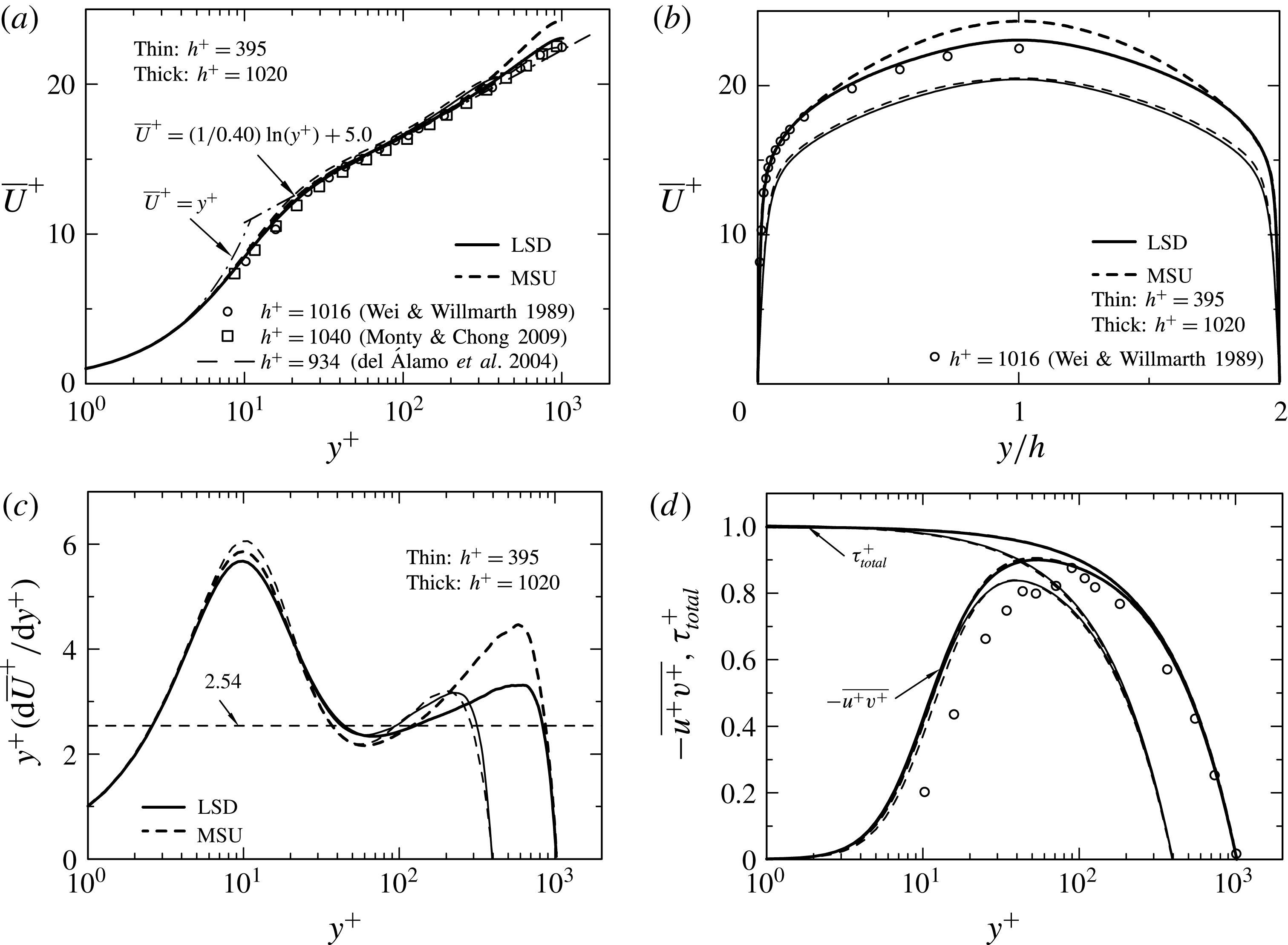
We first discuss the Re dependence of mean velocity and second-order moments in the MSU (i.e.
 ${L_{x}}^{+}\approx 400$
). The distributions of the normalized mean velocity
 $\overline{U}^{+}$
and Reynolds shear stress
 $-\overline{u^{+}v^{+}}$
for
 $h^{+}=395$
and 1020 are compared in figures 1(a) and 1(d) with those for the LSD (i.e.
 $L_{x}=12.8h$
). The experimental data of Wei & Willmarth (Reference Wei and Willmarth1989) and Monty et al. (Reference Monty, Stewart, Williams and Chong2007) and the DNS data of del Álamo et al. (Reference del Álamo, Jiménez, Zandonade and Moser2004) for the VLSD are also included. Overall agreement with the LSD is satisfactory for
 $h^{+}=395$
, while there is an increased magnitude of
 $\overline{U}^{+}$
for
 $h^{+}=1020$
in the outer region (
 $y^{+}>200$
, or equivalently,
 $y/h>0.2$
) of the MSU than for the LSD/VLSD (see also figure 1
b of where the near parabolic profile is observed in the distribution of
 $\overline{U}^{+}$
for the MSU). There is also the well-established logarithmic mean velocity distribution for the MSU, which is intrinsically associated with the spanwise organization of large-scale structures, as discussed in § 3.3. Note that whilst the distribution of
 $-\overline{u^{+}v^{+}}$
for the MSU agrees reasonably well with that of the LSD/VLSD and of the experiment by Wei & Willmarth (Reference Wei and Willmarth1989) (figure 1
d), there is a discernible difference in the mean velocity gradient between the MSU and LSD in the outer region (see figure 1
c where the magnitude of
 $y^{+}(\unicode[STIX]{x2202}\overline{U}^{+}/\unicode[STIX]{x2202}y^{+})$
for the MSU is larger in the outer region than for the LSD). The turbulent eddy viscosity
 $\unicode[STIX]{x1D708}_{t}\equiv -\overline{uv}/(\unicode[STIX]{x2202}\overline{U}/\unicode[STIX]{x2202}y)$
is thus smaller in the outer region of the MSU than for the LSD and exhibits near constancy (the distribution is not shown here), which was also observed in the simulations with both streamwise and spanwise minimal units by Jiménez & Pinelli (Reference Jiménez and Pinelli1999) up to
 $h^{+}=633$
. The present results are most likely associated with the increasing two-dimensionality of the LSMs with
 $h^{+}$
, as discussed below.
Distributions of
 $\overline{U}$
,
 $y(\unicode[STIX]{x2202}\overline{U}/\unicode[STIX]{x2202}y)$
and
 $-\overline{uv}$
normalized by wall units: (a,b)
 $\overline{U}^{+}$
; (c)
 $y^{+}(\unicode[STIX]{x2202}\overline{U}^{+}/\unicode[STIX]{x2202}y^{+})$
; (d)
 $-\overline{u^{+}v^{+}}$
. In (a,b), the distribution of
 $\overline{U}^{+}$
is shown in the half and whole channels, respectively. In (d), the distribution of the total shear stress,
 $\unicode[STIX]{x1D70F}_{total}^{+}=\unicode[STIX]{x2202}\overline{U}^{+}/\unicode[STIX]{x2202}y^{+}-\overline{u^{+}v^{+}}$
, is included. - - - - denotes the DNS data of del Álamo et al. (Reference del Álamo, Jiménez, Zandonade and Moser2004) for
 $h^{+}=934$
with the VLSD (
 $L_{x}=8\unicode[STIX]{x03C0}h$
). ○ and ▫ refer to the experimental data of Wei & Willmarth (Reference Wei and Willmarth1989) for
 $h^{+}=1016$
and of Monty & Chong (Reference Monty and Chong2009) for
 $h^{+}=1040$
.

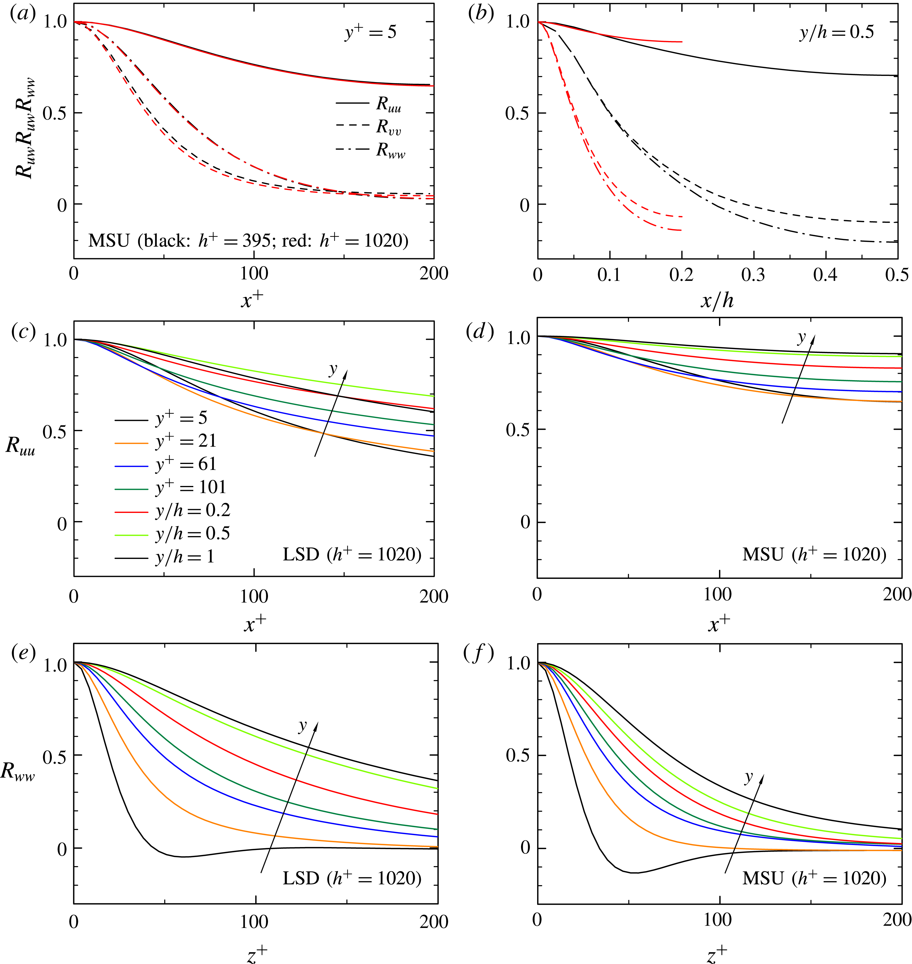
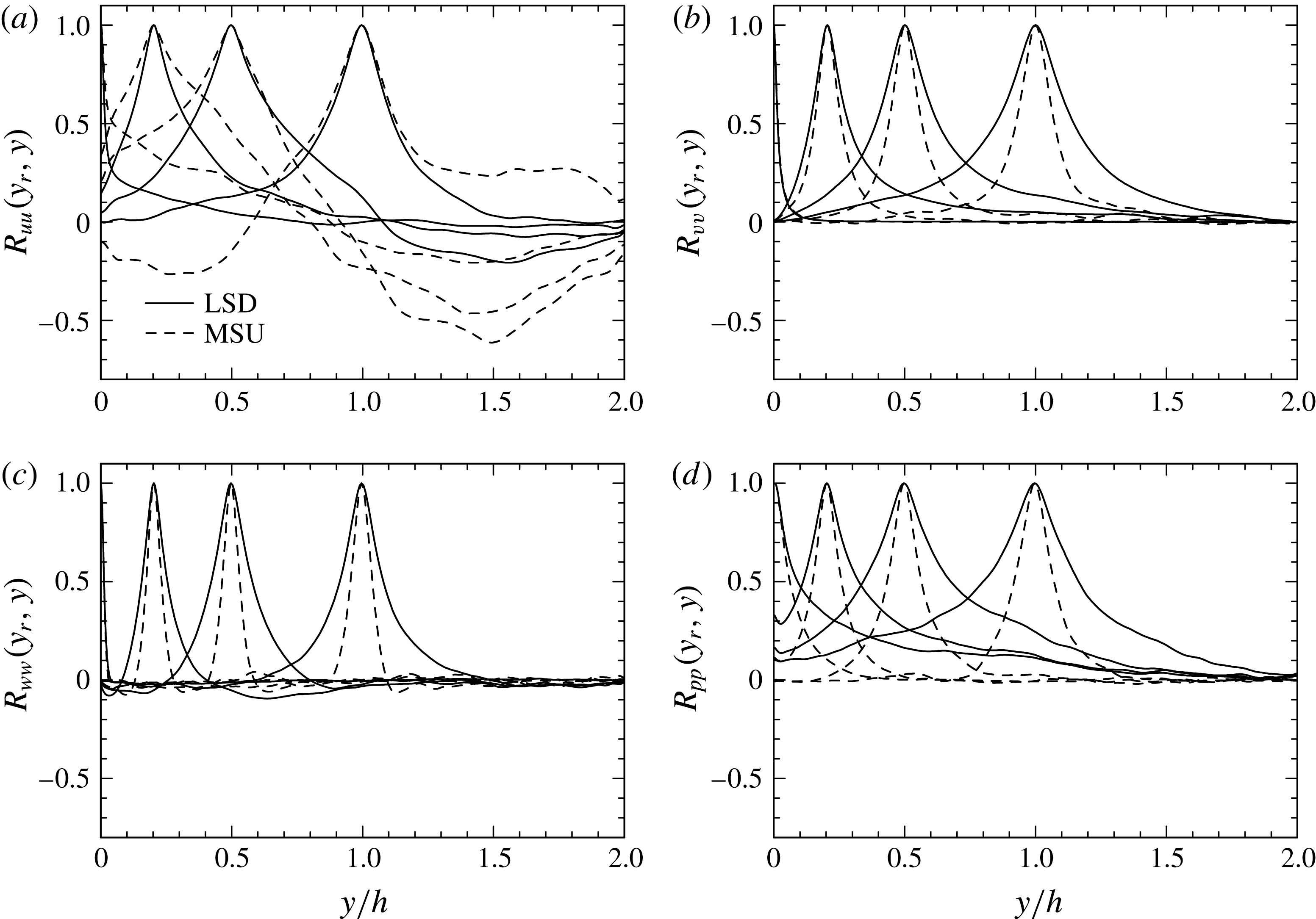
Streamwise and spanwise two-point correlations of velocity fluctuations: (a)
 $R_{uu}(\unicode[STIX]{x0394}x)$
,
 $R_{vv}(\unicode[STIX]{x0394}x)$
and
 $R_{ww}(\unicode[STIX]{x0394}x)$
for the MSU for
 $h^{+}=395$
and 1020 at
 $y^{+}=5$
; (b)
 $R_{uu}(\unicode[STIX]{x0394}x)$
,
 $R_{vv}(\unicode[STIX]{x0394}x)$
and
 $R_{ww}(\unicode[STIX]{x0394}x)$
for the MSU for
 $h^{+}=395$
and 1020 at
 $y/h=0.5$
; (c)
 $R_{uu}(\unicode[STIX]{x0394}x)$
for the LSD for
 $h^{+}=1020$
; (d)
 $R_{uu}(\unicode[STIX]{x0394}x)$
for the MSU for
 $h^{+}=1020$
; (e)
 $R_{ww}(\unicode[STIX]{x0394}z)$
for the LSD for
 $h^{+}=1020$
; (f)
 $R_{ww}(\unicode[STIX]{x0394}z)$
for the MSU for
 $h^{+}=1020$
. In (c–f), the
 $y$
locations of the plotted data are
 $y^{+}=5$
, 21, 61, 101 and
 $y/h=0.2$
, 0.5, 1.

Streamwise and spanwise two-point correlations are defined such that
 $$\begin{eqnarray}\displaystyle & \displaystyle R_{\unicode[STIX]{x1D6FC}\unicode[STIX]{x1D6FC}}(\unicode[STIX]{x0394}x)=\overline{\unicode[STIX]{x1D6FC}(\unicode[STIX]{x0394}x)\,\unicode[STIX]{x1D6FC}(x+\unicode[STIX]{x0394}x)}/\overline{\unicode[STIX]{x1D6FC}\unicode[STIX]{x1D6FC}} & \displaystyle\end{eqnarray}$$
and
 $$\begin{eqnarray}\displaystyle & \displaystyle R_{\unicode[STIX]{x1D6FC}\unicode[STIX]{x1D6FC}}(\unicode[STIX]{x0394}z)=\overline{\unicode[STIX]{x1D6FC}(\unicode[STIX]{x0394}z)\,\unicode[STIX]{x1D6FC}(z+\unicode[STIX]{x0394}z)}/\overline{\unicode[STIX]{x1D6FC}\unicode[STIX]{x1D6FC}}, & \displaystyle\end{eqnarray}$$
where
 $\unicode[STIX]{x1D6FC}\equiv u$
,
 $v$
or
 $w$
. Figures 2(a) and 2(b) show the distributions of
 $R_{uu}(\unicode[STIX]{x0394}x)$
,
 $R_{vv}(\unicode[STIX]{x0394}x)$
and
 $R_{ww}(\unicode[STIX]{x0394}x)$
in the inner and outer regions of the MSU for
 $h^{+}=395$
and 1020. Near the wall, the distributions remain invariably unchanged with
 $h^{+}$
. In the outer region (
 $y/h=0.5$
),
 $R_{uu}(\unicode[STIX]{x0394}x)$
for
 $h^{+}=1020$
shows a larger value (
 ${\approx}0.9$
) at the largest separation than that (
 ${\approx}0.7$
) for
 $h^{+}=395$
, whereas
 $R_{vv}(\unicode[STIX]{x0394}x)$
and
 $R_{ww}(\unicode[STIX]{x0394}x)$
for
 $h^{+}=1020$
show smaller values than those for
 $h^{+}=395$
. This indicates an increased two-dimensionality of
 $u$
in the outer region of the MSU at large
 $h^{+}$
. Panels 2(c) and 2(d) demonstrate how the magnitude of
 $R_{uu}(\unicode[STIX]{x0394}x)$
for
 $h^{+}=1020$
varies with increasing distance from the wall in the MSU and LSD. For the MSU,
 $R_{uu}(\unicode[STIX]{x0394}x)$
starts to show an increase in magnitude in the buffer region (
 $y^{+}>20$
) and exhibits a large value (
 ${\geqslant}0.8$
) in the outer region (
 $y/h>0.2$
) in which the distribution of
 $\overline{U}^{+}$
shows a larger value than that for the LSD. This highlights the close relationship between the two-dimensionality and the increased
 $\overline{U}^{+}$
in the outer region. Panels 2(e) and 2(f) show the distributions of
 $R_{ww}(\unicode[STIX]{x0394}z)$
for the MSU and LSD for
 $h^{+}=1020$
, which underline that the spanwise correlation of
 $w$
is reduced as a consequence of the two-dimensionality of large-scale structures. This behaviour is essentially associated with reduced spanwise meandering of the large-scale structures, as discussed in § 3.3.
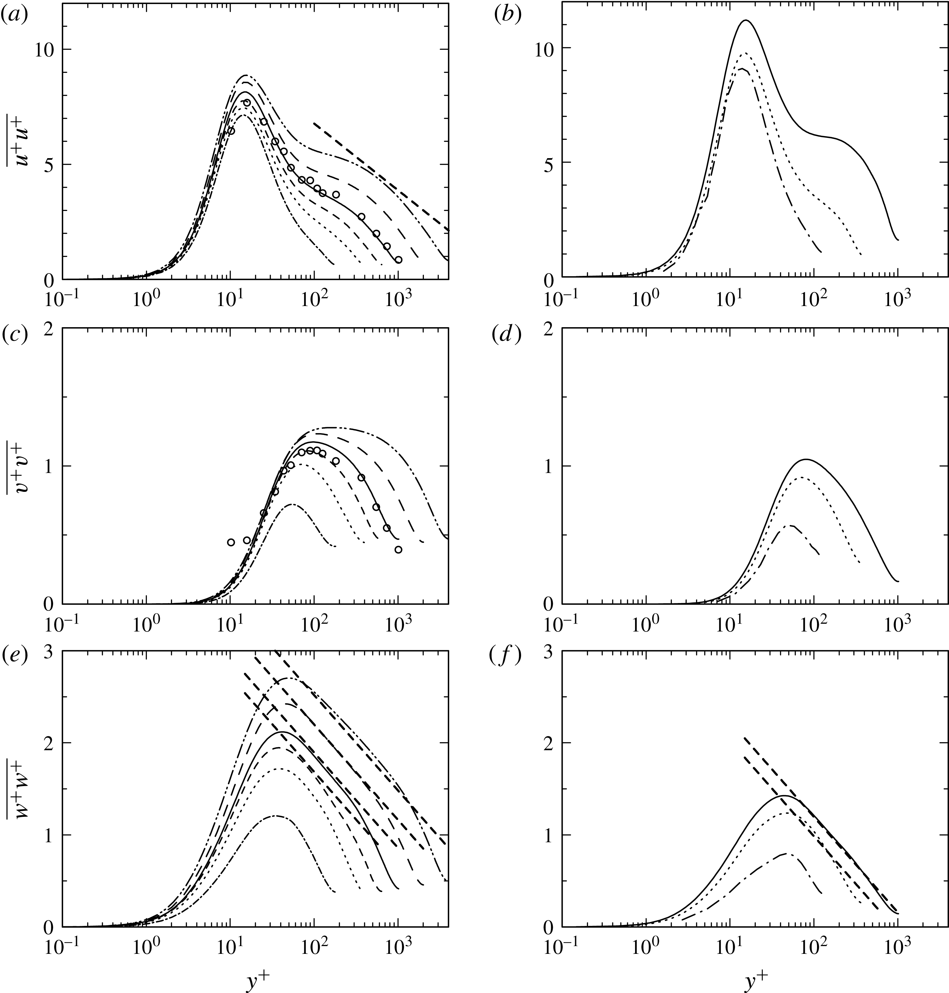
Figure 3 shows distributions of the Reynolds normal stresses (
 $\overline{u^{+}u^{+}}$
,
 $\overline{v^{+}v^{+}}$
,
 $\overline{w^{+}w^{+}}$
) for both the MSU and LSD. Unlike the wall-normal (
 $\overline{vv}$
) and tangential (
 $-\overline{uv}$
) Reynolds stresses (figures 3
c,d and 1
d), the two wall-parallel components
 $\overline{uu}$
and
 $\overline{ww}$
for the MSU (figure 3
b,f) are somewhat different from those for the LSD (figure 3
a,e). Indeed, the magnitude of
 $\overline{uu}$
becomes more energetic as
 $h^{+}$
increases. In particular, there is almost a plateau instead of a large outer peak in
 $\overline{uu}$
when
 $h^{+}$
reaches 1020. The latter magnitude is comparable with that for the VLSD at
 $h^{+}=4000$
(Bernardini et al.
Reference Bernardini, Pirozzoli and Orlandi2014), which indicates the presence of energized LSMs in the MSU for a large
 $h^{+}$
(see § 3.3). On the other hand, the magnitude of
 $\overline{ww}$
for the MSU decreases significantly away from the wall. In high Re wall-bounded turbulent flows, the attached eddy model (Townsend Reference Townsend1976; Perry, Henbest & Chong Reference Perry, Henbest and Chong1986) predicts a logarithmic dependence for the two wall-parallel Reynolds stresses, viz.
 $$\begin{eqnarray}\displaystyle & \displaystyle \overline{uu}/U_{\unicode[STIX]{x1D70F}}^{2}=A_{1}-B_{1}\ln (y/h) & \displaystyle\end{eqnarray}$$
and
 $$\begin{eqnarray}\displaystyle & \displaystyle \overline{ww}/U_{\unicode[STIX]{x1D70F}}^{2}=A_{3}-B_{3}\ln (y/h), & \displaystyle\end{eqnarray}$$
where
 $A_{1}$
,
 $A_{3}$
,
 $B_{1}$
,
 $B_{3}$
are constants, while
 $\overline{vv}/U_{\unicode[STIX]{x1D70F}}^{2}\simeq \text{constant}$
and
 $-\overline{uv}/U_{\unicode[STIX]{x1D70F}}^{2}=1$
(see also figures 3
c,d and 1
d). Recently, it has become evident that
 $\overline{ww}/U_{\unicode[STIX]{x1D70F}}^{2}$
exhibits a logarithmic dependence even below
 $h^{+}=2000$
where, like
 $\overline{U}^{+}$
,
 $\overline{uu}/U_{\unicode[STIX]{x1D70F}}^{2}$
shows a departure from the logarithmic dependence due to very long and wide eddies in
 $u$
indicated by Jiménez & Hoyas (Reference Jiménez and Hoyas2008) (note that the profiles corresponding to (3.3) and (3.4) with
 $A_{1}=2.1$
,
 $A_{3}=0.85$
,
 $B_{1}=1.26$
,
 $B_{3}=0.45$
are plotted as ‘bold dashed lines’ in figures 3
a and 3
e). Figure 3 indicates that while the magnitude of
 $\overline{ww}$
for the MSU is attenuated, it exhibits a clearer logarithmic dependence than for the LSD (see figure 3
f where (3.4) with
 $A_{3}=0.15$
,
 $B_{3}=0.45$
is plotted and the agreement is convincing for the MSU when
 $h^{+}=1020$
). This behaviour is most likely associated with reduced spanwise large scales in
 $w$
for the MSU (see figure 10
f) since small scales are likely to ‘lose’ the Re dependence more rapidly than large scales (see Abe & Antonia Reference Abe and Antonia2016, Reference Abe and Antonia2017 who noted that the overlap scaling for the energy and scalar dissipation rates is in fact established at a smaller value of
 $h^{+}$
than that at which the mean velocity and scalar log laws hold). Like
 $\overline{uu}/U_{\unicode[STIX]{x1D70F}}^{2}$
(see Jiménez & Hoyas Reference Jiménez and Hoyas2008),
 $\overline{ww}/U_{\unicode[STIX]{x1D70F}}^{2}$
is contaminated by the large-scale inactive motion. The attenuated spanwise large scales, associated with
 $w$
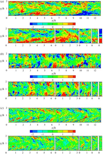
, essentially result from the fact that the LSMs have three-dimensional shear layers (see the x–y contours in figure 4
c and the y–z contours in figure 10
e,f), i.e. backs. In this context, Robinson (Reference Robinson1991) classified structures in a turbulent boundary layer into eight categories and noted that ‘backs’ are large-scale shear-layer interfaces between high (positive
 $u$
) and low (negative
 $u$
) speed fluid (i.e. sloping delta-scale discontinuities in the streamwise velocity) (see also figure 4
a). This will be further discussed in § 3.2, with a focus on the relationship with the pressure fluctuations (figure 4
b) and spanwise velocity fluctuations (figure 4
c).
Distributions of normalized mean-square velocity fluctuations: (a,b)
 $\overline{uu}/U_{\unicode[STIX]{x1D70F}}^{2}$
; (c,d)
 $\overline{vv}/U_{\unicode[STIX]{x1D70F}}^{2}$
; (e,f)
 $\overline{ww}/U_{\unicode[STIX]{x1D70F}}^{2}$
. The data for the LSD are plotted in (a,c,e) together with those for the VLSDs in the literature, whereas those for the MSU are given in (b,d,f). In (a,c,e), – ⋅ – ⋅ –,
 $h^{+}=180$
;
 $\cdots \cdots$
,
 $h^{+}=395$
; - - - -,
 $h^{+}=640$
; ——,
 $h^{+}=1020$
; – – – –,
 $h^{+}=2003$
(Hoyas & Jiménez Reference Hoyas and Jiménez2008); — ⋅ ⋅ —,
 $h^{+}=4079$
(Bernardini et al.
Reference Bernardini, Pirozzoli and Orlandi2014); ○, Wei & Willmarth (Reference Wei and Willmarth1989) for
 $h^{+}=1016$
. The bold dashed-lines in (a) and (e) come from relations of (3.3) and (3.4), respectively, with
 $A_{1}=2.1$
,
 $A_{3}=0.85$
,
 $B_{1}=1.26$
,
 $B_{3}=0.45$
, while those in (f) are from (3.4) with
 $A_{3}=0.15$
,
 $B_{3}=0.45$
. In (b,d,f), – ⋅ – ⋅ –,
 $h^{+}=137$
(Toh & Itano Reference Toh and Itano2005);
 $\cdots \cdots$
,
 $h^{+}=395$
; ——,
 $h^{+}$
 $=1020$
.

Contours in the
 $x$
–
 $y$
plane of instantaneous
 $u$
,
 $p$
and
 $w$
for
 $h^{+}=1020$
: (a)
 $u$
; (b)
 $p$
; (c)
 $w$
. In each panel, the top section shows the data for
 $L_{x}=12.8h$
(LSD), whereas the bottom section shows the data for
 $L_{x}=6.4h$
,
 $L_{x}=3.2h$
,
 $L_{x}=1.6h$
,
 $L_{x}=0.8h$
and
 $L_{x}=0.4h$
(MSU), the order being from left to right. In the top panel, the black solid lines have inclinations of 10 (left line) and 20 (right line) degrees.

3.2 Effect of varying
 $L_{x}$

In this subsection, we discuss how turbulence statistics and structures vary with decreasing
 $L_{x}$
for a sufficiently large Kármán number
 $h^{+}$
so that the inner and outer regions are sufficiently separated. Figure 4 shows contours of instantaneous streamwise velocity fluctuations
 $u$
in the
 $x$
–
 $y$
plane for
 $h^{+}=1020$
. Also included are contours of the instantaneous pressure fluctuations
 $p$
and spanwise velocity fluctuations
 $w$
. For the LSD (
 $L_{x}=12.8h$
), large-scale
 $u$
structures with a streamwise inclination of 10 to 20 degrees dominate in the outer region (see the two solid lines in figure 4
a), where positive and negative
 $p$
structures appear at the edge of negative
 $u$
structures (see the two solid lines in figure 4
b). This observation is consistent with the presence of transverse vortices along the edge of streamwise inclined negative
 $u$
structures (e.g. the PIV (particle image velocimetry) measurements of Christensen & Adrian Reference Christensen and Adrian2001 in connection with hairpin vortex packets and the DNS analysis of VLSMs by Lee & Sung Reference Lee and Sung2011). The streamwise inclination of the large-scale structures however becomes smaller with decreasing
 $L_{x}$
when
 $L_{x}<6.4h$
, which is intrinsically associated with the streamwise extent of the LSMs (i.e. approximately
 $2\sim 4h$
) (see Balakumar & Adrian Reference Balakumar and Adrian2007). For the MSU (i.e.
 ${L_{x}}^{+}\approx 400$
), the
 $u$
structures indeed exhibit a two-dimensional behaviour in the outer region, consistent with the result for the streamwise two-point correlations shown in figure 2(d).
Effect of varying
 $L_{x}$
on premultiplied one-dimensional streamwise spectra of
 $u$
,
 $k_{x}\unicode[STIX]{x1D719}_{uu}(k_{x})$
, normalized by
 $U_{\unicode[STIX]{x1D70F}}^{2}$
for
 $h^{+}=1020$
: (a)
 $y/h=0.1$
; (b)
 $y/h=0.3$
; (c)
 $y/h=0.5$
; (d)
 $y/h=0.7$
. – – – – denotes the DNS data of del Álamo et al. (Reference del Álamo, Jiménez, Zandonade and Moser2004) for
 $h^{+}=934$
with the VLSD (
 $L_{x}=8\unicode[STIX]{x03C0}h$
). ○ and ▫ refer to the experimental data of Balakumar & Adrian (Reference Balakumar and Adrian2007) for
 $h^{+}=960$
and of Monty & Chong (Reference Monty and Chong2009) for
 $h^{+}=1040$
.

Effect of varying
 $L_{x}$
on streamwise two-point correlations of
 $u$
,
 $R_{uu}(\unicode[STIX]{x0394}x)$
, for
 $h^{+}=1020$
: (a)
 $y/h=0.1$
; (b)
 $y/h=0.3$
; (c)
 $y/h=0.5$
; (d)
 $y/h=0.7$
.

The streamwise variation of the large-scale
 $u$
structures may be quantified by the energy spectra. One-dimensional streamwise and spanwise spectra are defined such that
 $$\begin{eqnarray}\displaystyle & \displaystyle \int _{0}^{\infty }\unicode[STIX]{x1D719}_{\unicode[STIX]{x1D6FC}\unicode[STIX]{x1D6FC}}(k_{x})\,\text{d}k_{x}=\int _{0}^{\infty }k_{x}\unicode[STIX]{x1D719}_{\unicode[STIX]{x1D6FC}\unicode[STIX]{x1D6FC}}(k_{x})\,\text{d}(\log k_{x})=\overline{\unicode[STIX]{x1D6FC}\unicode[STIX]{x1D6FC}} & \displaystyle\end{eqnarray}$$
and
 $$\begin{eqnarray}\displaystyle & \displaystyle \int _{0}^{\infty }\unicode[STIX]{x1D719}_{\unicode[STIX]{x1D6FC}\unicode[STIX]{x1D6FC}}(k_{z})\,\text{d}k_{z}=\int _{0}^{\infty }k_{x}\unicode[STIX]{x1D719}_{\unicode[STIX]{x1D6FC}\unicode[STIX]{x1D6FC}}(k_{z})\,\text{d}(\log k_{z})=\overline{\unicode[STIX]{x1D6FC}\unicode[STIX]{x1D6FC}}, & \displaystyle\end{eqnarray}$$
where
 $\unicode[STIX]{x1D719}$
denotes the one-dimensional spectral density,
 $k_{x}$
and
 $k_{z}$
the streamwise and spanwise wavenumbers,
 $\unicode[STIX]{x1D706}_{x}(=2\unicode[STIX]{x03C0}/k_{x})$
and
 $\unicode[STIX]{x1D706}_{z}(=2\unicode[STIX]{x03C0}/k_{z})$
being the corresponding wavelengths and
 $\unicode[STIX]{x1D6FC}\equiv u$
,
 $v$
,
 $w$
or
 $p$
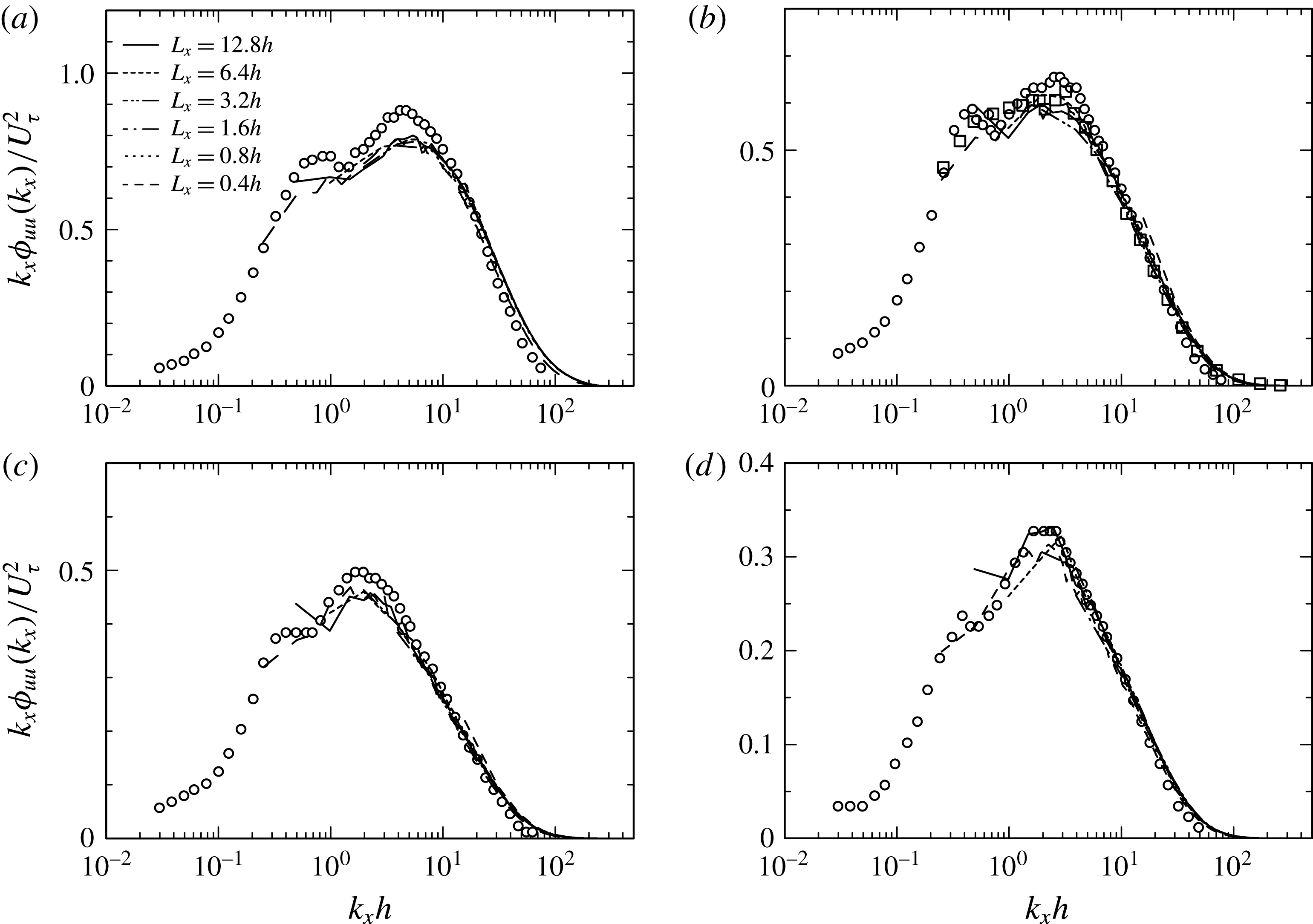
. Figure 5 shows the streamwise
 $u$
spectra
 $\unicode[STIX]{x1D719}_{uu}(k_{x})$
normalized by
 $U_{\unicode[STIX]{x1D70F}}^{2}$
at several
 $y$
stations in the outer region (viz.
 $y/h=0.1$
, 0.3, 0.5 and 0.7). Also included are the experimental data of Balakumar & Adrian (Reference Balakumar and Adrian2007) for
 $h^{+}=960$
and of Monty & Chong (Reference Monty and Chong2009) for
 $h^{+}=1040$
and the DNS data for the VLSD of del Álamo et al. (Reference del Álamo, Jiménez, Zandonade and Moser2004) for
 $h^{+}=934$
. Whilst the streamwise
 $u$
spectra for the MSU agree reasonably well with those for the larger
 $L_{x}$
and also for the experiments up to their smallest non-zero wavenumbers, the most energetic outer spectral peak appearing at
 $k_{x}h=1.5{-}3$
(i.e.
 $\unicode[STIX]{x1D706}_{x}/h=2{-}4$
) is not reproduced when
 $L_{x}<6.4h$
. The latter criterion of
 $L_{x}=6.4h$
is identical with the finding of Lozano-Durán & Jiménez (Reference Lozano-Durán and Jiménez2014) that correct one-point statistics are obtained when
 $L_{x}$
is larger than
 $2\unicode[STIX]{x03C0}h$
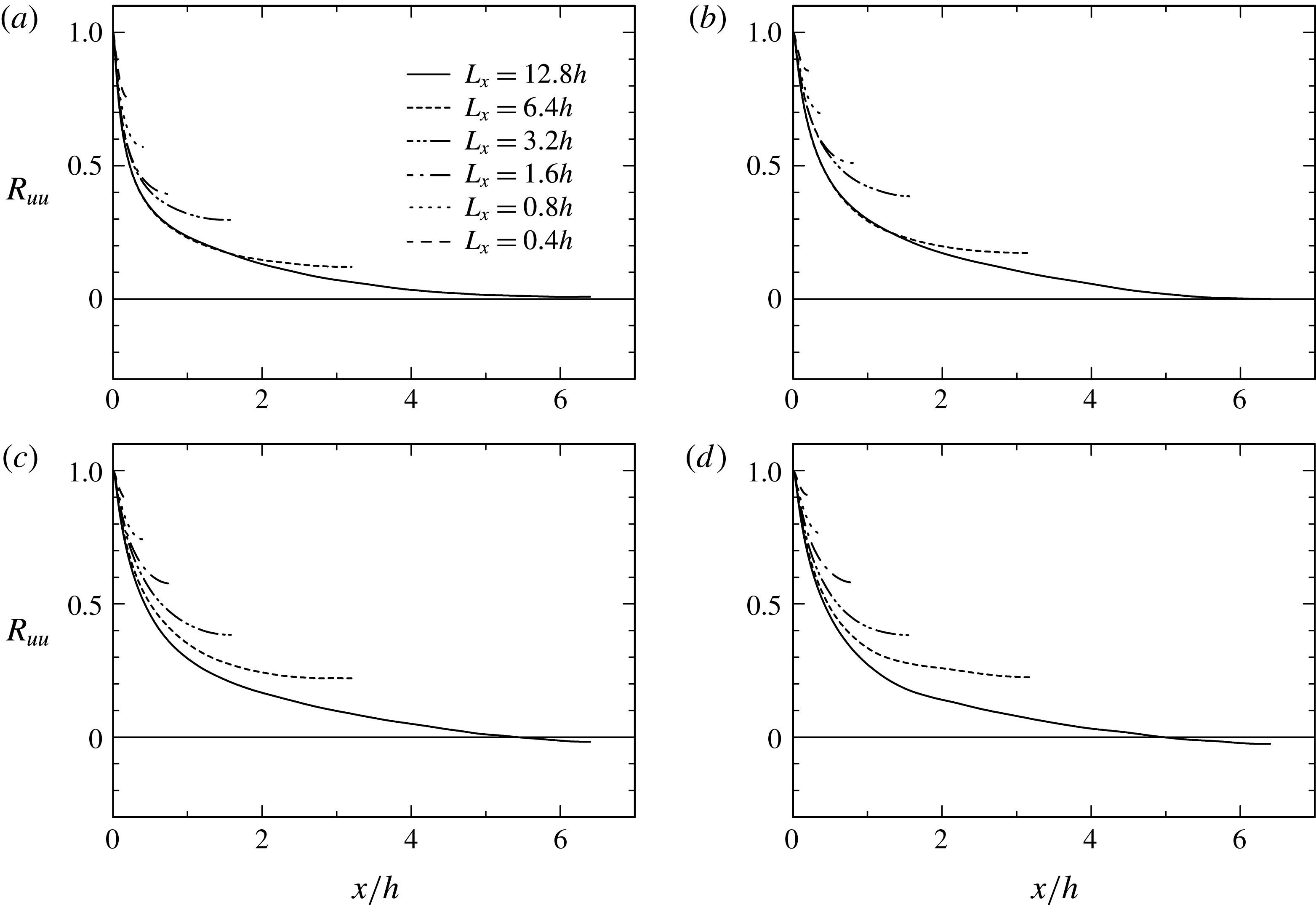
. Also shown in figure 6 is the variation with
 $L_{x}$
of the streamwise two-point correlations of
 $u$
in the outer region (viz.
 $y/h=0.1$
, 0.3, 0.5 and 0.7). The correlation at the largest separation becomes smaller as
 $L_{x}$
increases. The present result is associated with the streamwise organization of the LSMs as observed in figure 4(a), which needs to be taken into account in order to reproduce correctly one-point statistics of velocity and pressure fluctuations (this will be discussed below). We also note a discernible difference in the streamwise
 $u$
spectra between the LSD and VLSD in the outer region where the low-wavenumber peak is resolved in the VLSD, but not in the LSD (see figure 5). This peak wavelength corresponds to the streamwise extent of the VLSMs (see Balakumar & Adrian Reference Balakumar and Adrian2007). The spanwise
 $u$
spectra however do not exhibit a noticeable difference between the LSD and VLSD (see figures 12
a,b and 16
a); mean and second-order statistics are also identical between the LSD and VLSD (see figures 1
a and 7).
Effect of varying
 $L_{x}$
on the mean-square velocity and pressure fluctuations for
 $h^{+}=1020$
: (a)
 $\overline{uu}/U_{\unicode[STIX]{x1D70F}}^{2}$
; (b)
 $\overline{ww}/U_{\unicode[STIX]{x1D70F}}^{2}$
; (c)
 $\overline{vv}/U_{\unicode[STIX]{x1D70F}}^{2}$
; (d)
 $\overline{pp}/\unicode[STIX]{x1D70F}_{w}^{2}$
. - - - - denotes the DNS data of del Álamo et al. (Reference del Álamo, Jiménez, Zandonade and Moser2004) for
 $h^{+}=934$
with the VLSD (
 $L_{x}=8\unicode[STIX]{x03C0}h$
). ▫ refers to the experimental data of Monty & Chong (Reference Monty and Chong2009) for
 $h^{+}=1040$
. In (b,d), the bold dashed-lines are based on relations (3.4) with
 $A_{3}=0.85$
,
 $B_{3}=0.45$
and (3.7), respectively.

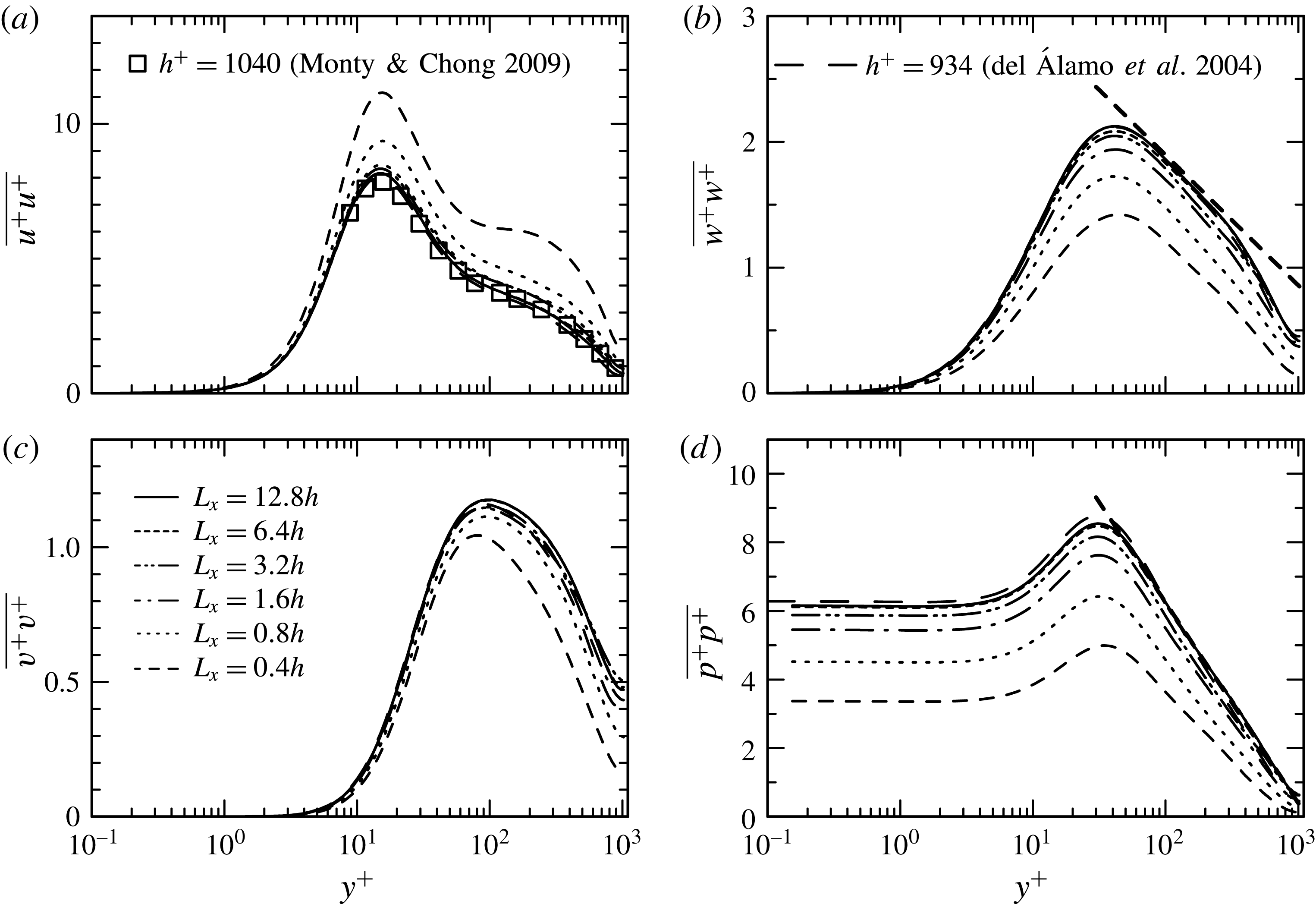
Figure 7 illustrates the
 $L_{x}$
dependence of the Reynolds normal stresses (
 $\overline{uu}$
,
 $\overline{vv}$
,
 $\overline{ww}$
) and mean-square pressure fluctuations (
 $\overline{pp}$
). Clearly, the magnitude of
 $\overline{uu}/U_{\unicode[STIX]{x1D70F}}^{2}$
increases with decreasing
 $L_{x}$
, whereas the magnitudes of
 $\overline{vv}/U_{\unicode[STIX]{x1D70F}}^{2}$
,
 $\overline{ww}/U_{\unicode[STIX]{x1D70F}}^{2}$
and
 $\overline{pp}/\unicode[STIX]{x1D70F}_{w}^{2}$
decrease with decreasing
 $L_{x}$
. This behaviour is essentially linked to the weakened energy redistribution (see figure 9
e). In particular, the rate of decrease in
 $\overline{ww}/U_{\unicode[STIX]{x1D70F}}^{2}$
and
 $\overline{pp}/\unicode[STIX]{x1D70F}_{w}^{2}$
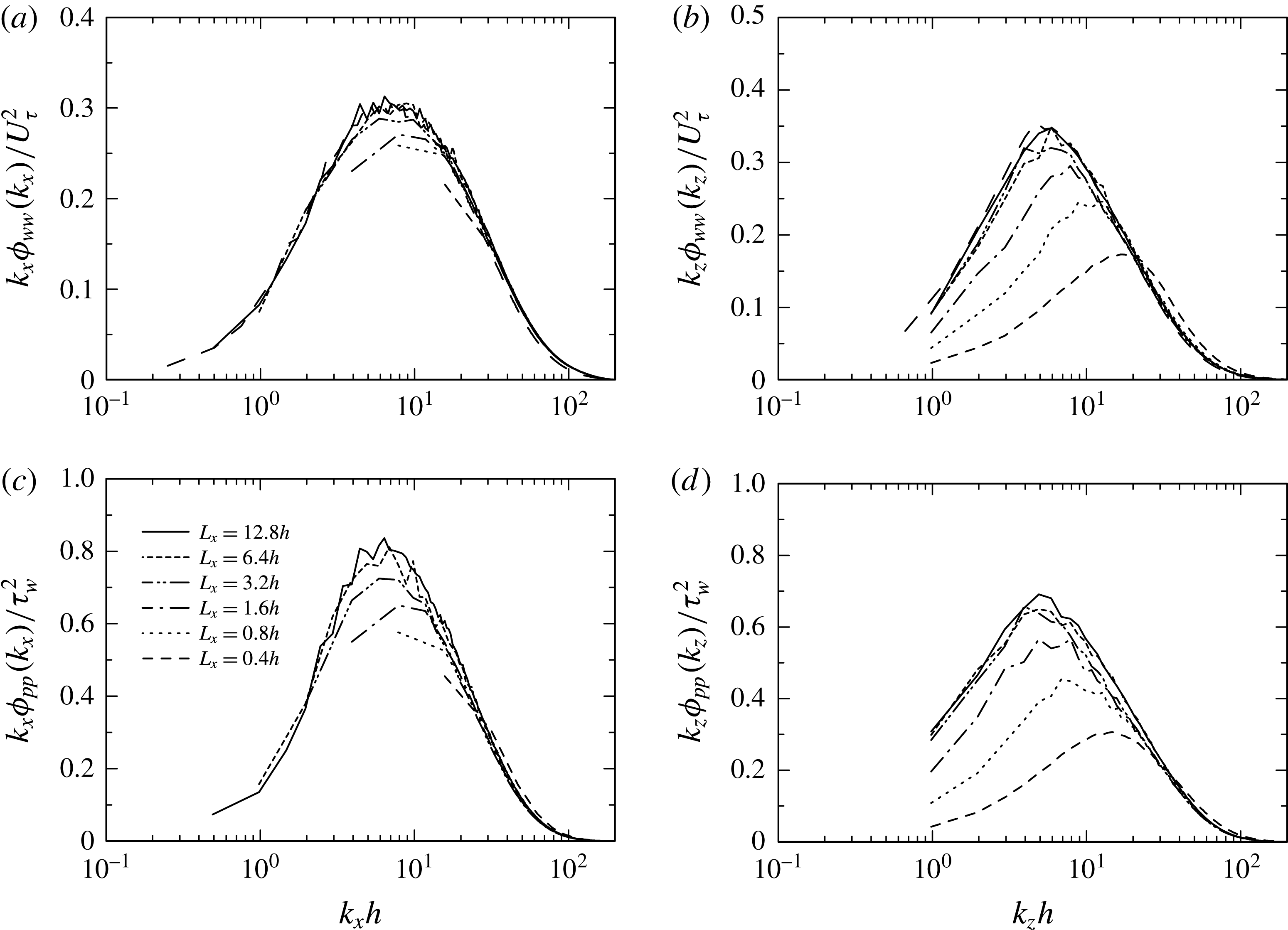
is large. Figure 8 shows the premultiplied streamwise and spanwise spectra of
 $w$
and
 $p$
in the outer region (
 $y/h=0.5$
) for
 $h^{+}=1020$
. Both the streamwise and spanwise spectra are attenuated at large wavelengths when
 $L_{x}$
is below 6.4
 $h$
. In the streamwise spectra, there is a close similarity between the
 $w$
and
 $p$
spectra, consistent with the good similarity in the instantaneous contours in the x–y plane of
 $w$
and
 $p$
(see figure 4
b,c where the sloping
 $w$
structures related to three-dimensional shear layers and the pressure structures associated with transverse vortices are observed). On the other hand, the spanwise
 $w$
spectra show more prominent peaks than the spanwise
 $p$
spectra. Indeed, there is a discernible difference in the peak wavelengths (
 $\unicode[STIX]{x1D706}_{z,max}$
) of the
 $w$
and
 $p$
spectra shown in figures 12(c) and 12(d) where the
 $p$
spectra for the LSD show a wider
 $y$
range of the linear increase of
 $\unicode[STIX]{x1D706}_{z,max}$
than the
 $w$
spectra. The latter corresponds to a wider
 $y$
region of the logarithmic dependence of
 $\overline{pp}/\unicode[STIX]{x1D70F}_{w}^{2}$
than that of
 $\overline{ww}/U_{\unicode[STIX]{x1D70F}}^{2}$
(see figure 7
b,d). The instantaneous contours in the y–z plane of
 $w$
and
 $p$
for the LSD (see figures 10
e and 19
a) also show some differences:
 $w$
displays spanwise large-scale structures while
 $p$
exhibits smaller-scale structures than
 $w$
. This result corroborates the finding of Jiménez & Hoyas (Reference Jiménez and Hoyas2008) that because of the lack of very large scales, the pressure fluctuations away from the wall scale very well with
 $\unicode[STIX]{x1D70C}U_{\unicode[STIX]{x1D70F}}^{2}$
(or equivalently,
 $\unicode[STIX]{x1D70F}_{w}$
). When
 $L_{x}<6.4h$
, the three-dimensional shear layers are not represented properly due to the less resolved streamwise behaviour of the LSMs where the pressure fluctuations exhibit localized structures (see § 3.4). Indeed, the peak wavelengths of both the spanwise
 $w$
and
 $p$
spectra for the MSU show a wide
 $y$
range of linear increase, consistent with the better logarithmic dependence of
 $\overline{ww}/U_{\unicode[STIX]{x1D70F}}^{2}$
for the MSU. This underlines that spanwise large scales is responsible for the departure from the logarithmic dependence of
 $\overline{ww}/U_{\unicode[STIX]{x1D70F}}^{2}$
.
Effect of varying
 $L_{x}$
on premultiplied one-dimensional streamwise and spanwise spectra of
 $w$
and
 $p$
for
 $h^{+}=1020$
at
 $y/h=0.5$
: (a)
 $k_{x}\unicode[STIX]{x1D719}_{ww}(k_{x})/U_{\unicode[STIX]{x1D70F}}^{2}$
; (b)
 $k_{z}\unicode[STIX]{x1D719}_{ww}(k_{z})/U_{\unicode[STIX]{x1D70F}}^{2}$
; (c)
 $k_{x}\unicode[STIX]{x1D719}_{pp}(k_{x})/\unicode[STIX]{x1D70F}_{w}^{2}$
; (d)
 $k_{z}\unicode[STIX]{x1D719}_{pp}(k_{z})/\unicode[STIX]{x1D70F}_{w}^{2}$
. In (a,b), – – – – denotes the DNS data of del Álamo et al. (Reference del Álamo, Jiménez, Zandonade and Moser2004) for
 $h^{+}=934$
with the VLSD (
 $L_{x}=8\unicode[STIX]{x03C0}h$
).

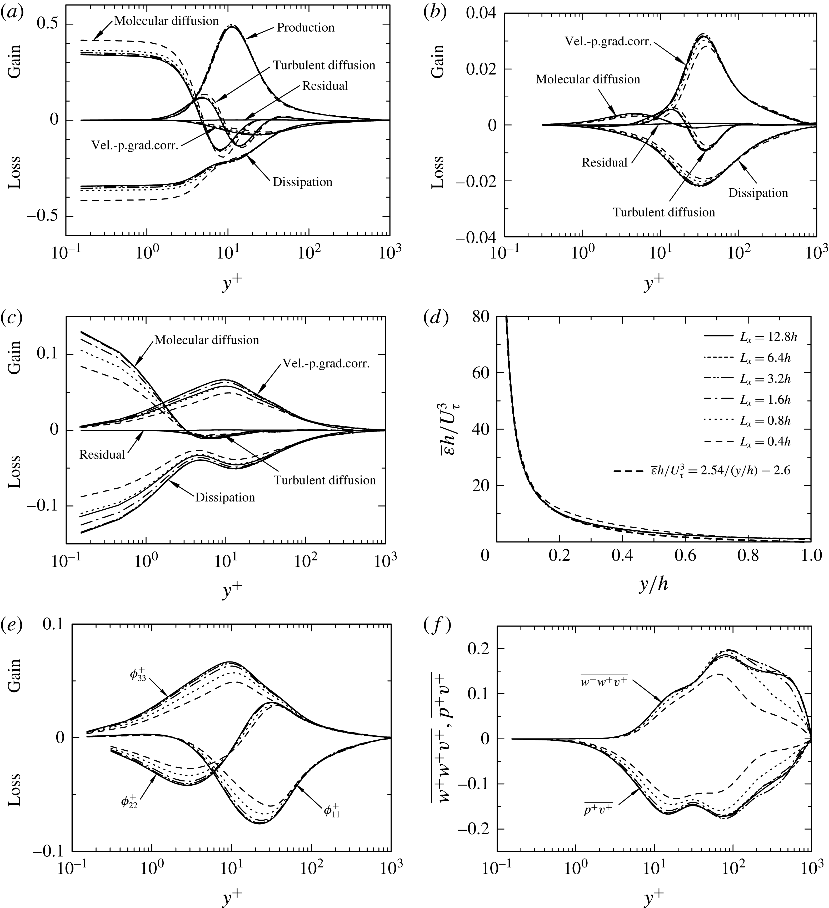
Effect of varying
 $L_{x}$
on budgets of the Reynolds normal stresses, energy dissipation rate, pressure strain and diffusion terms for
 $h^{+}=1020$
: (a) budget of
 $\overline{uu}$
; (b) budget of
 $\overline{vv}$
; (c) budget of
 $\overline{ww}$
; (d)
 $\overline{\unicode[STIX]{x1D700}}h/U_{\unicode[STIX]{x1D70F}}^{3}$
; (e)
 $\unicode[STIX]{x1D719}_{11}^{+}$
,
 $\unicode[STIX]{x1D719}_{22}^{+}$
and
 $\unicode[STIX]{x1D719}_{33}^{+}$
; (f)
 $\overline{w^{+}w^{+}v^{+}}$
and
 $\overline{v^{+}p^{+}}$
. In (a–c), the normalization has been made by
 $U_{\unicode[STIX]{x1D70F}}^{4}/\unicode[STIX]{x1D708}$
. In (d), the bold dashed-line denotes the relation
 $\overline{\unicode[STIX]{x1D700}}h/U_{\unicode[STIX]{x1D70F}}^{3}=2.54/(y/h)-2.6$
, which is equivalent to relation (3.9) or (3.10).

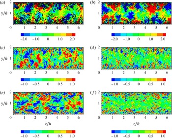
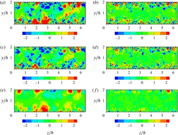
Contours in the
 $y$
–
 $z$
plane of instantaneous streamwise, wall-normal and spanwise velocity fluctuations,
 $u$
,
 $v$
,
 $w$
, for
 $h^{+}=1020$
: (a,b)
 $u$
; (c,d)
 $v$
; (e,f)
 $w$
. (a,c,e) Correspond to the LSD (
 $L_{x}=12.8h$
), while (b,d,f) are for the MSU (
 ${L_{x}}^{+}\approx 400$
). In (a,b), lines denote positive values of the second invariant of
 $Q^{+}$
(line contour levels are from
 $5\times 10^{-4}$
to
 $5\times 10^{-3}$
with an increment of
 $5\times 10^{-5}$
).

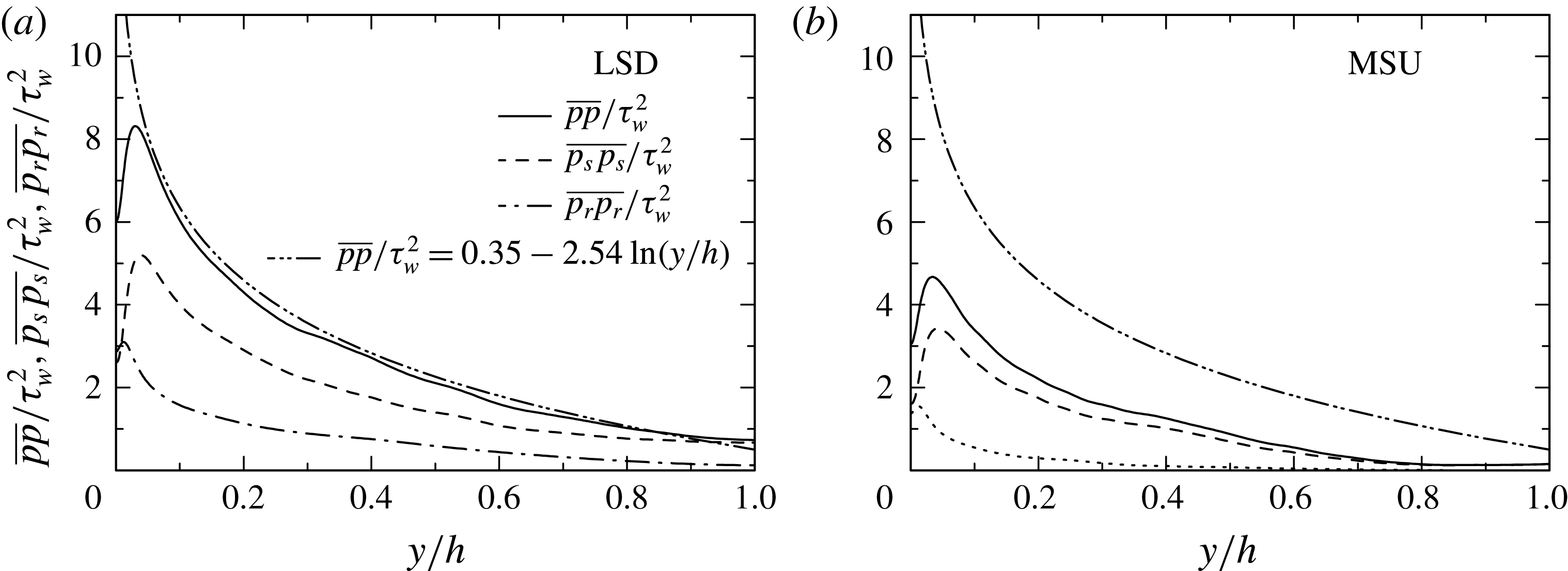
The dependence of
 $\overline{pp}$
may be expressed as
 $$\begin{eqnarray}\displaystyle & \displaystyle \overline{pp}/\unicode[STIX]{x1D70F}_{w}^{2}=0.35-2.54\ln (y/h) & \displaystyle\end{eqnarray}$$
(note that the profile corresponding to (3.7) is plotted as a ‘bold dashed line’ in figure 7
d). Recently, Panton, Lee & Moser (Reference Panton, Lee and Moser2017) obtained an analogous relation to (3.7) by using matching argument. They found an interesting similarity between the slope of (3.7) and the magnitude of the von Kármán constant
 $\unicode[STIX]{x1D705}$
. They mentioned that ‘the physics governing the mean velocity and the pressure fluctuations is quite different’ but they did not point out that there is in fact a close similarity between (3.7) and what has been observed (Abe & Antonia Reference Abe and Antonia2016) for
 $\overline{\unicode[STIX]{x1D700}}$
. In this context, Poisson’s equation suggests a close relationship between the pressure derivative and energy dissipation rate (see Bradshaw & Koh Reference Bradshaw and Koh1981), although their characteristic
 $y$
scales are different (this difference was pointed out by one of the referees; see also the wall-normal two-point correlations for
 $p$
shown in figure 18
d). Abe & Antonia (Reference Abe and Antonia2016) found that the mean energy dissipation rate, i.e.
 $$\begin{eqnarray}\displaystyle & \displaystyle \overline{\unicode[STIX]{x1D700}}=\unicode[STIX]{x1D708}\overline{u_{i,j}(u_{i,j}+u_{j,i})}, & \displaystyle\end{eqnarray}$$
has an analogous overlap scaling,
 $$\begin{eqnarray}\displaystyle & \displaystyle \overline{\unicode[STIX]{x1D700}}y/U_{\unicode[STIX]{x1D70F}}^{3}=1/\unicode[STIX]{x1D705}_{\unicode[STIX]{x1D700}}-c(y^{+}/h^{+}) & \displaystyle\end{eqnarray}$$
and
 $$\begin{eqnarray}\displaystyle & \displaystyle \overline{\unicode[STIX]{x1D700}}y/U_{\unicode[STIX]{x1D70F}}^{3}=1/\unicode[STIX]{x1D705}_{\unicode[STIX]{x1D700}}-c(y/h), & \displaystyle\end{eqnarray}$$
with
 $1/\unicode[STIX]{x1D705}_{\unicode[STIX]{x1D700}}=2.54$
and
 $c=2.6$
(see figure 9
d). The magnitude of
 $1/\unicode[STIX]{x1D705}_{\unicode[STIX]{x1D700}}$
is identical to that of the slope in (3.7). In our previous studies (Abe & Antonia Reference Abe and Antonia2016, Reference Abe and Antonia2017) on the energy and passive-scalar dissipation rates, we noted that the overlap region for the dissipation is more readily established than that for the mean fields since the small scales (i.e. dissipation) are likely to ‘lose’ their dependence on the Reynolds number more rapidly than the large scales. Since small scales make up the source term in Poisson’s equation and the outer-layer similarity for both
 $\overline{pp}$
and
 $\overline{\unicode[STIX]{x1D700}}$
is established at much smaller
 $h^{+}$
than that for
 $\bar{U}$
, it seems reasonable to identify the scaling behaviour of
 $\overline{pp}$
with that of
 $\overline{\unicode[STIX]{x1D700}}$
. Note that unlike
 $\overline{pp}$
, the scaling for
 $\overline{\unicode[STIX]{x1D700}}$
is essentially unaffected by
 $L_{x}$
. This is because
 $\overline{pp}$
has wall-attached global nature (see the wall-normal two-point correlation of
 $p$
shown in figure 18
d), whilst
 $\overline{\unicode[STIX]{x1D700}}$
is essentially a small-scale quantity. When
 $h^{+}$
is sufficiently large (
 ${\geqslant}5000$
) for the velocity log law to be established over a region where
 $P_{k}\simeq \overline{\unicode[STIX]{x1D700}}$
and
 $-\overline{uv}\simeq \text{const.}$
(see figure 10 of Abe & Antonia Reference Abe and Antonia2016), the von Kármán constant
 $\unicode[STIX]{x1D705}$
can be identified with
 $\unicode[STIX]{x1D705}_{\unicode[STIX]{x1D700}}$
. Consistent with the similarity between
 $w$
and
 $p$
discussed above, the logarithmic dependence of
 $\overline{ww}/U_{\unicode[STIX]{x1D70F}}^{2}$
is also established for a lower Kármán number than that at which the mean velocity log law is first observed. The lower
 $y$
bound of the logarithmic dependence of
 $\overline{ww}/U_{\unicode[STIX]{x1D70F}}^{2}$
and
 $\overline{pp}/\unicode[STIX]{x1D70F}_{w}^{2}$
is indeed smaller than that of
 $\bar{U}$
, which indicates that
 $\overline{ww}/U_{\unicode[STIX]{x1D70F}}^{2}$
and
 $\overline{pp}/\unicode[STIX]{x1D70F}_{w}^{2}$
are less affected by viscous effects. An analogous trend was observed in a turbulent boundary layer by Spalart (Reference Spalart1988). In his simulations, the viscous correction obtained by Perry et al. (Reference Perry, Henbest and Chong1986) was successfully applied to
 $\overline{ww}$
rather than
 $\overline{uu}$
.
To gain further insight into the
 $L_{x}$
dependence of the Reynolds normal stresses, we examine the transport equation of
 $\overline{u_{i}u_{j}}$
defined such that
 $$\begin{eqnarray}\displaystyle & \displaystyle 0=P_{ij}+T_{ij}+\unicode[STIX]{x1D6F1}_{ij}+D_{ij}-\unicode[STIX]{x1D700}_{ij}, & \displaystyle\end{eqnarray}$$
where
 $$\begin{eqnarray}\displaystyle & \displaystyle P_{ij}^{+}=-\overline{u_{j}^{+}u_{k}^{+}}{\displaystyle \frac{\unicode[STIX]{x2202}\overline{U}_{i}^{+}}{\unicode[STIX]{x2202}x_{k}^{+}}}-\overline{u_{i}^{+}u_{k}^{+}}{\displaystyle \frac{\unicode[STIX]{x2202}\overline{U}_{j}^{+}}{\unicode[STIX]{x2202}x_{k}^{+}}}, & \displaystyle\end{eqnarray}$$
 $$\begin{eqnarray}\displaystyle & \displaystyle T_{ij}^{+}=-{\displaystyle \frac{\unicode[STIX]{x2202}}{\unicode[STIX]{x2202}x_{k}^{+}}}\overline{u_{i}^{+}u_{j}^{+}u_{k}^{+}}, & \displaystyle\end{eqnarray}$$
 $$\begin{eqnarray}\displaystyle & \displaystyle \unicode[STIX]{x1D6F1}_{ij}^{+}=-\overline{u_{j}^{+}{\displaystyle \frac{\unicode[STIX]{x2202}p^{+}}{\unicode[STIX]{x2202}x_{i}^{+}}}}-\overline{u_{i}^{+}{\displaystyle \frac{\unicode[STIX]{x2202}p^{+}}{\unicode[STIX]{x2202}x_{j}^{+}}}}, & \displaystyle\end{eqnarray}$$
 $$\begin{eqnarray}\displaystyle & \displaystyle D_{ij}^{+}={\displaystyle \frac{\unicode[STIX]{x2202}^{2}}{\unicode[STIX]{x2202}x_{k}^{+2}}}\overline{u_{i}^{+}u_{j}^{+}}, & \displaystyle\end{eqnarray}$$
 $$\begin{eqnarray}\displaystyle & \displaystyle \overline{\unicode[STIX]{x1D700}_{ij}}^{+}=2\overline{{\displaystyle \frac{\unicode[STIX]{x2202}u_{i}^{+}}{\unicode[STIX]{x2202}x_{k}^{+}}}{\displaystyle \frac{\unicode[STIX]{x2202}u_{j}^{+}}{\unicode[STIX]{x2202}x_{k}^{+}}}}. & \displaystyle\end{eqnarray}$$
 $P_{ij}^{+}$
,
 $T_{ij}^{+}$
,
 $\unicode[STIX]{x1D6F1}_{ij}^{+}$
,
 $D_{ij}^{+}$
and
 $\overline{\unicode[STIX]{x1D700}_{ij}}^{+}$
denote the production, turbulent diffusion, velocity-pressure-gradient correlation (VPG), molecular diffusion, homogeneous dissipation, respectively. Figure 9(a–c) shows budgets of
 $\overline{uu}$
,
 $\overline{vv}$
,
 $\overline{ww}$
non-dimensionalized by
 $U_{\unicode[STIX]{x1D70F}}^{4}/\unicode[STIX]{x1D708}$
, which demonstrate the significant
 $L_{x}$
dependence of the spanwise Reynolds stress. For the
 $\overline{uu}$
budget, the production is essentially independent of
 $L_{x}$
, whereas the magnitudes of molecular diffusion and dissipation increase with decreasing
 $L_{x}$
close to the wall (figure 9
a). The
 $L_{x}$
independence of the production essentially comes from the forcing by the mean pressure gradient. As
 $L_{x}$
decreases,
 $\overline{\unicode[STIX]{x1D700}_{11}}$
increases whereas
 $\overline{\unicode[STIX]{x1D700}_{33}}$
decreases (figure 9
a,c) but the energy dissipation rate
 $\overline{\unicode[STIX]{x1D700}}$
(
 $\equiv \overline{\unicode[STIX]{x1D700}_{ii}}/2$
) is basically unchanged (figure 9
d). The total amount of energy (both produced and dissipated) is thus essentially unchanged. In the energy balance (i.e. integrals of the
 $k$
budget across the channel), the integral of the production is thus balanced by that of the dissipation since the integrals of convection and diffusion terms become zero. The latter relationship is satisfied independently of
 $L_{x}$
(see also section 2 of Abe & Antonia Reference Abe and Antonia2016). As for the turbulent flux, the turbulent diffusion terms (
 $T_{22}^{+}$
,
 $T_{33}^{+}$
) and the VPG ones (
 $\unicode[STIX]{x1D6F1}_{11}^{+}$
,
 $\unicode[STIX]{x1D6F1}_{22}^{+}$
,
 $\unicode[STIX]{x1D6F1}_{33}^{+}$
) decrease as
 $L_{x}$
decreases. The VPG term may be split into the pressure strain
 $\unicode[STIX]{x1D719}_{ij}^{+}$
and pressure diffusion
 $\unicode[STIX]{x1D711}_{ij}^{+}$
, respectively, i.e.
 $$\begin{eqnarray}\displaystyle & \displaystyle \unicode[STIX]{x1D6F1}_{ij}^{+}=\underbrace{\overline{p^{+}\left({\displaystyle \frac{\unicode[STIX]{x2202}u_{i}^{+}}{\unicode[STIX]{x2202}x_{j}^{+}}}+{\displaystyle \frac{\unicode[STIX]{x2202}u_{j}^{+}}{\unicode[STIX]{x2202}x_{i}^{+}}}\right)}}_{\unicode[STIX]{x1D719}_{ij}^{+}}\underbrace{-\left({\displaystyle \frac{\unicode[STIX]{x2202}}{\unicode[STIX]{x2202}x_{i}^{+}}}\overline{u_{j}^{+}p^{+}}+{\displaystyle \frac{\unicode[STIX]{x2202}}{\unicode[STIX]{x2202}x_{j}^{+}}}\overline{u_{i}^{+}p^{+}}\right)}_{\unicode[STIX]{x1D711}_{ij}^{+}}. & \displaystyle\end{eqnarray}$$
The pressure strain plays a role in redistributing the energy from
 $\overline{uu}$
to
 $\overline{vv}$
and
 $\overline{ww}$
. Note that
 $\unicode[STIX]{x1D719}_{11}^{+}$
and
 $\unicode[STIX]{x1D719}_{33}^{+}$
are equivalent to
 $\unicode[STIX]{x1D6F1}_{11}^{+}$
and
 $\unicode[STIX]{x1D6F1}_{33}^{+}$
, respectively, in the present flow. Figure 9(e) demonstrates that there is a weakened energy redistribution (see also Abe & Antonia Reference Abe and Antonia2016). For
 $L_{x}<6.4h$
, the magnitudes of
 $\unicode[STIX]{x1D719}_{11}^{+}$
and
 $\unicode[STIX]{x1D719}_{33}^{+}$
are attenuated significantly for
 $y^{+}<100$
due to the impaired global nature of the pressure (see also the wall-normal two-point correlations of
 $p$
shown in figure 18
d). Consistent with the behaviour of
 $T_{33}^{+}$
and
 $\unicode[STIX]{x1D6F1}_{22}^{+}$
, the energy fluxes of
 $\overline{w^{+}w^{+}v^{+}}$
and
 $\overline{p^{+}v^{+}}$
are also reduced noticeably across the channel when
 $L_{x}$
is small (see figure 9
f). This reflects the weakened turbulent diffusion resulting from the two-dimensionality in the MSU. This behaviour is essentially associated with more energized large-scale
 $u$
structures in the MSU than in the LSD (see figure 10
a,b), which is consistent with the increase in the mean streamwise velocity (see the near parabolic profile in figure 1
b). The magnitudes of
 $\overline{vv}$
and
 $\overline{ww}$
(figure 7
b,c) hence become smaller when
 $L_{x}$
decreases. The present observation for the MSU is consistent with the expectation of SSP at large Reynolds numbers (Waleffe & Kim Reference Waleffe, Kim and Panton1997). In particular, two wall-parallel components (
 $\overline{uu}$
and
 $\overline{ww}$
) are affected significantly by varying
 $L_{x}$
due to the absence of two properties of the large-scale structures, namely their streamwise inclination and spanwise meandering (the latter will be discussed further in the next subsection).
3.3 Spanwise organization of velocity fluctuations
Here, we discuss the spanwise organization of velocity fluctuations for the MSU and LSD (i.e.
 $L_{x}=0.4h$
and
 $12.8h$
) for
 $h^{+}=1020$
. Contours of instantaneous streamwise, wall-normal and spanwise velocity fluctuations (
 $u$
,
 $v$
,
 $w$
) in the
 $y$
–
 $z$
plane for
 $h^{+}=1020$
are shown in figure 10. This figure underlines the presence of hierarchical
 $u$
structures for both the MSU and LSD. Clearly, the spanwise organization of streamwise velocity fluctuations
 $u$
is essentially identical between the two cases, whilst wall-normal and spanwise velocity fluctuations
 $v$
and
 $w$
away from the wall are weakened as
 $L_{x}$
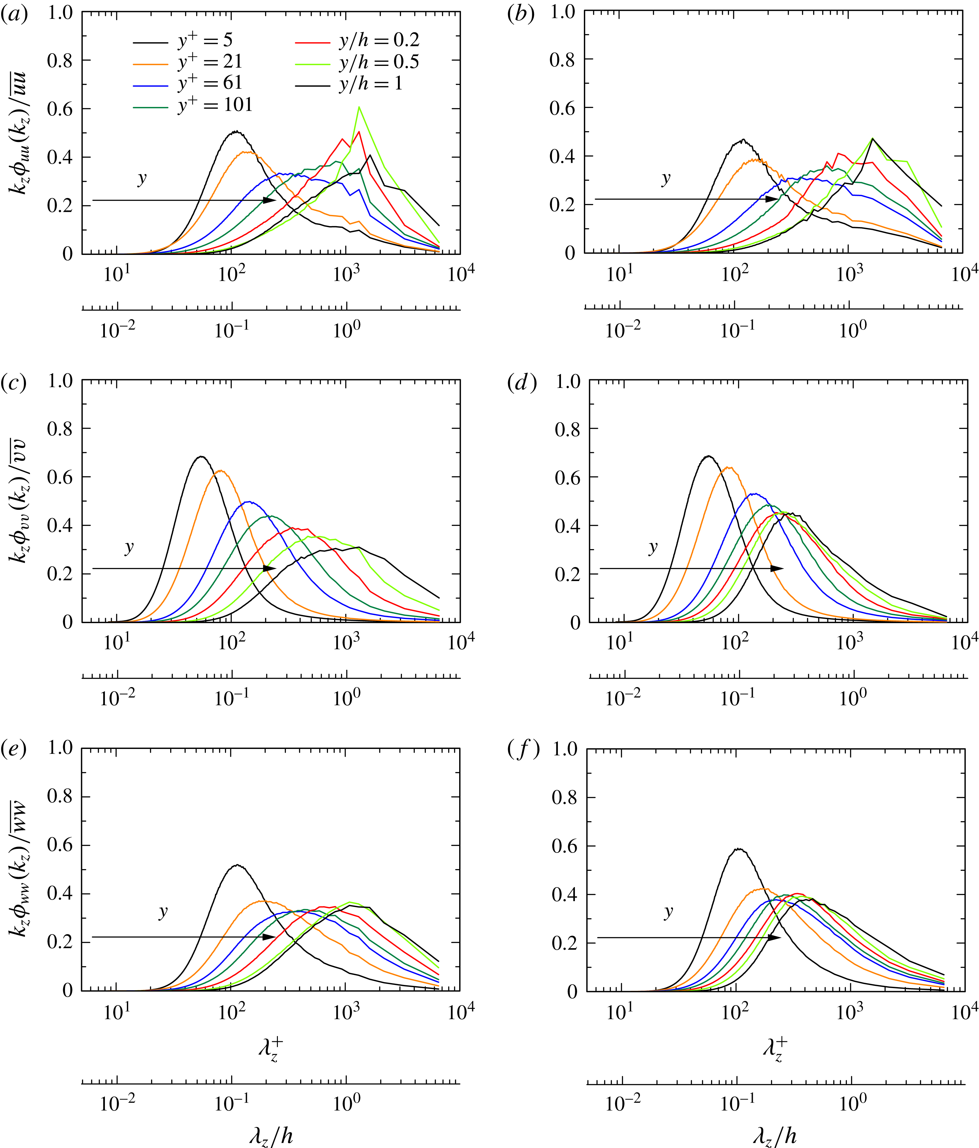
decreases. These behaviours are supported statistically by figure 11 where the premultiplied spanwise spectra of
 $u$
,
 $v$
,
 $w$
are shown at several
 $y$
locations. Indeed, the MSU reproduces the spanwise organization of large-scale structures in the log region properly even at sufficiently large
 $h^{+}$
, consistent with the well-established logarithmic mean velocity distribution (see figure 1
a). One discernible difference from the LSD is that large-scale structures in the outer region (
 $y/h>0.2$
) are more energized for the MSU due to the reduced turbulent diffusion resulting from the approach of the large-scale structures towards the two-dimensionality (see figure 9
f); consequently, a large majority of the turbulent kinetic energy (approximately 80 %) is carried by the large-scale
 $u$
structures in the MSU. The negative
 $u$
structures (see figure 10
a,b where the positive values of the second invariant of the velocity gradient tensor
 $Q(\equiv -u_{i,j}u_{j,i}/2)$
are also depicted as a vortex indicator and preferably associated with the negative
 $u$
structures in the outer region) are also closely associated with negative uv regions as for the LSD and active in the context of the momentum transport (the instantaneous product of
 $u$
and
 $v$
is not shown here). The latter underlines that the infinitely long
 $u$
structures observed for the MSU are responsible for the increase in the mean velocity distribution in the outer region (see the near parabolic profile in figure 1
b).
One-dimensional premultiplied spanwise spectra of
 $u$
,
 $v$
and
 $w$
for
 $h^{+}=1020$
: (a,b)
 $k_{z}\unicode[STIX]{x1D719}_{uu}(k_{z})/\overline{uu}$
; (c,d)
 $k_{z}\unicode[STIX]{x1D719}_{vv}(k_{z})/\overline{vv}$
; (e,f)
 $k_{z}\unicode[STIX]{x1D719}_{ww}(k_{z})/\overline{ww}$
. (a,c,e) Correspond to the LSD (
 $L_{x}=12.8h$
), while (b,d,f) are for the MSU (
 ${L_{x}}^{+}\approx 400$
). In each figure, the
 $y$
locations of the plotted data are
 $y^{+}=5$
, 21, 61, 101 and
 $y/h=0.2$
, 0.5, 1.

Most energetic spanwise scales,
 $\unicode[STIX]{x1D706}_{z,max}$
, obtained from peaks of premultiplied spanwise spectra of
 $u$
,
 $w$
and
 $p$
for the MSU and LSD
 $h^{+}=1020$
: (a),
 $\unicode[STIX]{x1D706}_{z,max}/h$
for
 $u$
(b)
 $\unicode[STIX]{x1D706}_{z,max}^{+}$
for
 $u$
; (c)
 $\unicode[STIX]{x1D706}_{z,max}/h$
for
 $w$
; (d)
 $\unicode[STIX]{x1D706}_{z,max}/h$
for
 $p$
. In (a,b), ▫ denotes the DNS data of del Álamo et al. (Reference del Álamo, Jiménez, Zandonade and Moser2004) for
 $h^{+}=934$
with the VLSD (
 $L_{x}=8\unicode[STIX]{x03C0}h$
). In (a); the dashed, one-dotted and two-dotted lines denote
 $\unicode[STIX]{x1D706}_{z,max}/h=0.8$
, 1.3 and 1.6, respectively; the ‘diamonds’ refer to the data of Tomkins & Adrian (Reference Tomkins and Adrian2005) in a zero-pressure-gradient turbulent boundary layer for
 $\unicode[STIX]{x1D6FF}^{+}=426$
. In (b–d), the dashed lines are linear fits to the data.

We now examine the most energetic spanwise scales of the hierarchical
 $u$
structures,
 $\unicode[STIX]{x1D706}_{z,max}$
, by plotting the peak wavelengths of the premultiplied spectra
 $k_{z}\unicode[STIX]{x1D719}_{uu}(k_{z})$
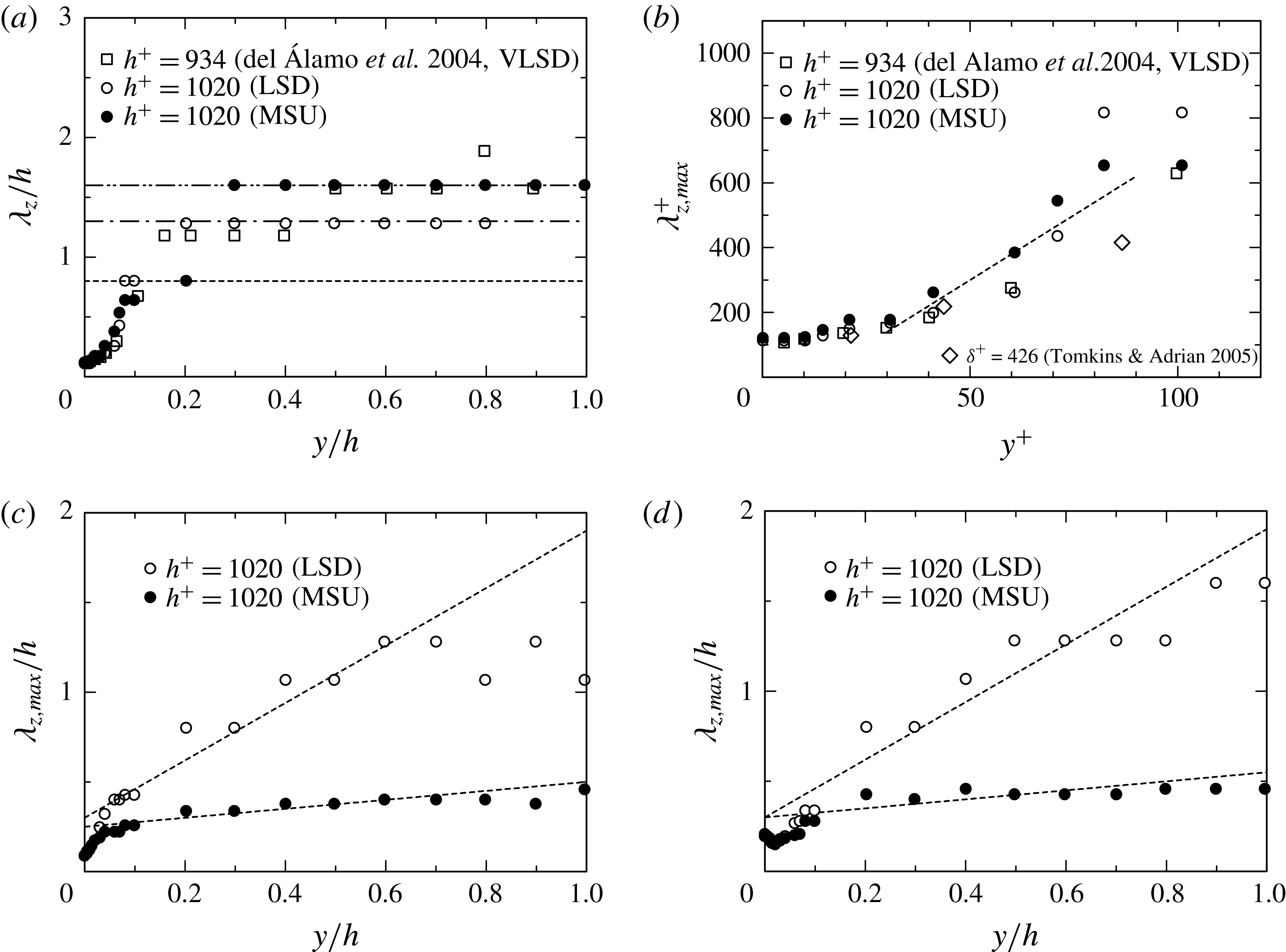
shown in figure 11(a,b). Note that the peak wavelength of the premultiplied spectrum corresponds to the most energetic scale contributing to the mean square value. Figure 12(a) demonstrates that there are three energetic spanwise scales for both the MSU and LSD, which are essentially identical to those for the VLSD of del Álamo et al. (Reference del Álamo, Jiménez, Zandonade and Moser2004). Near the wall, a large peak appears at
 ${\unicode[STIX]{x1D706}_{z}}^{+}\approx 100$
, which corresponds to mean spanwise spacing of near-wall streaks (Smith & Metzler Reference Smith and Metzler1983). Away from the wall, the most energetic spanwise scales tend to increase linearly with distance from the wall in the range
 $40\leqslant y^{+}\leqslant 80$
(see figure 12
b), which is consistent with the approximate self-similarity of the energetic spanwise scales and agrees well with the experimental results (Nakagawa & Nezu Reference Nakagawa and Nezu1977; Smith & Metzler Reference Smith and Metzler1983; Tomkins & Adrian Reference Tomkins and Adrian2003, Reference Tomkins and Adrian2005). The linear increase in
 $\unicode[STIX]{x1D706}_{z,max}$
is better observed for the
 $w$
and
 $p$
spectra (see figure 12
c,d). Here,
 $\unicode[STIX]{x1D706}_{z,max}$
associated with
 $w$
shows a linear increase over a wider range of
 $y$
for the MSU than for the LSD. The
 $y$
range of the linear increase corresponds well to that for the logarithmic dependence of
 $\overline{ww}/U_{\unicode[STIX]{x1D70F}}^{2}$
. This implies that the departure from the logarithmic behaviour of
 $\overline{ww}/U_{\unicode[STIX]{x1D70F}}^{2}$
is essentially associated with the large-scale spanwise meandering observed in the LSD/VLSD, which corroborates Jiménez & Hoyas’s (Reference Jiménez and Hoyas2008) finding that most of the departure from the logarithmic behaviour of
 $\overline{uu}/U_{\unicode[STIX]{x1D70F}}^{2}$
is due to the very long and wide eddies in
 $u$
. Given the notion of Nickels et al. (Reference Nickels, Marusic, Hafez, Hutchins and Chong2007) that any eddy with a size that scales with its distance from the wall may be considered to be attached to the wall, the well-established logarithmic dependence of
 $\overline{ww}/U_{\unicode[STIX]{x1D70F}}^{2}$
in the MSU is intrinsically associated with the attached eddy hypothesis of Townsend (Reference Townsend1976). On the other hand, the
 $\unicode[STIX]{x1D706}_{z}/h=1.3\sim 1.6$
peak dominates in the outer region (
 $y/h=0.2{-}1$
) (see figure 12
a), which corresponds to the outer global mode (del Álamo & Jiménez Reference del Álamo and Jiménez2003; Abe et al.
Reference Abe, Kawamura and Choi2004b
; Bernardini et al.
Reference Bernardini, Pirozzoli and Orlandi2014). The present result indicates that while the outer global modes are observed in the longest and widest modes of the
 $u$
spectra (i.e.
 $\unicode[STIX]{x1D706}_{x}/h>5\sim 6h$
and
 $\unicode[STIX]{x1D706}_{z}/h>1\sim 2h$
) for the VLSD (Jiménez & Hoyas Reference Jiménez and Hoyas2008), the MSU and LSD also capture the spanwise global mode in the spectra. This underlines that the spanwise organization of the VLSMs can be represented approximately as infinitely long structures.
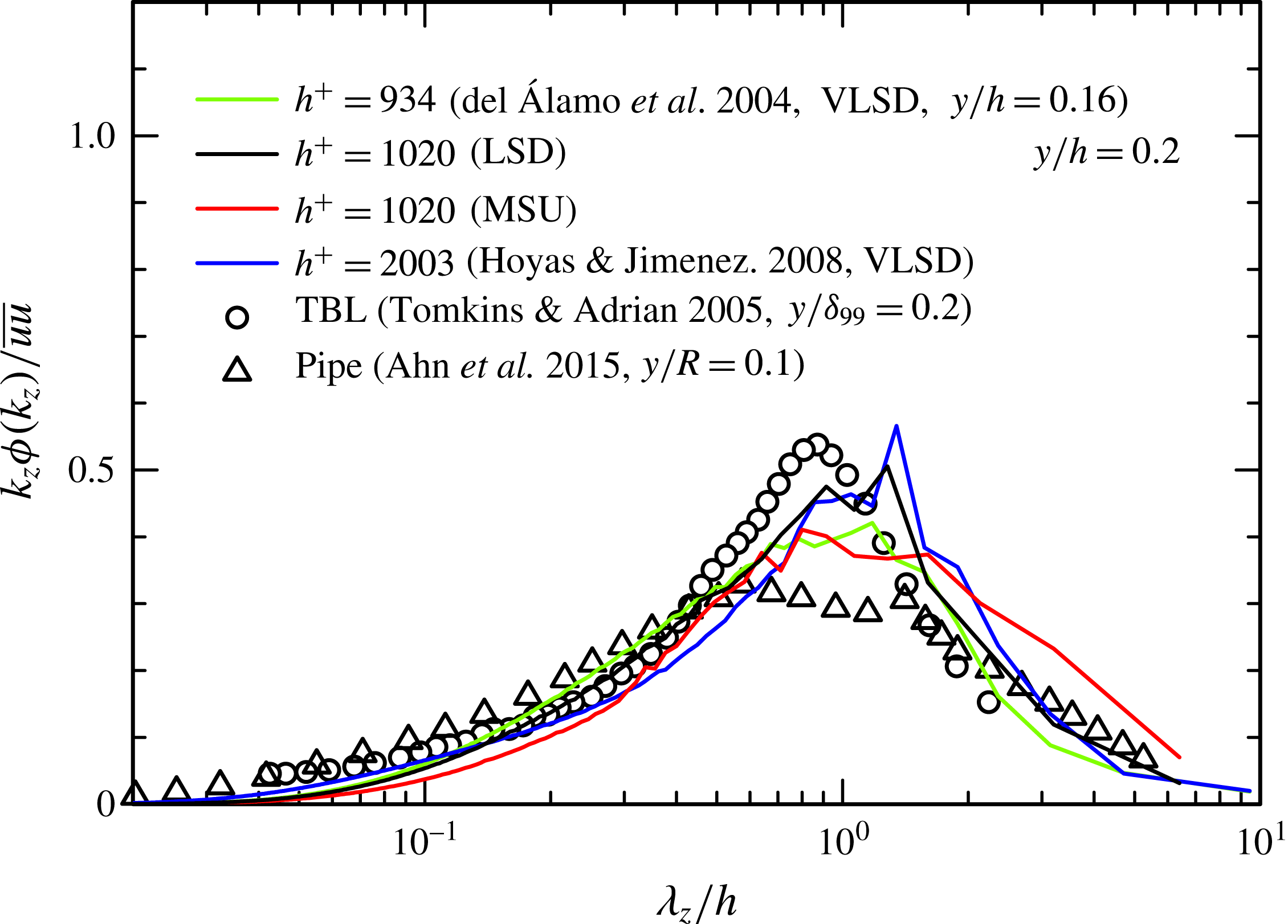
One-dimensional premultiplied spanwise spectra of
 $u$
for
 $h^{+}=1020$
for the LSD (the black line) and MSU (the red line) at
 $y/h=0.2$
. The spectra are compared with those of del Álamo et al. (Reference del Álamo, Jiménez, Zandonade and Moser2004) and Hoyas & Jiménez (Reference Hoyas and Jiménez2008) for
 $h^{+}=934$
and 2003 at
 $y/h=0.16$
(the green line) and
 $y/h=0.2$
(the blue line), respectively, for the VLSD (
 $L_{x}=8\unicode[STIX]{x03C0}h$
) in the present flow. Also included are the spectra of Tomkins & Adrian (Reference Tomkins and Adrian2005) in a zero-pressure-gradient turbulent boundary layer for
 $\unicode[STIX]{x1D6FF}^{+}=2216$
at
 $y/\unicode[STIX]{x1D6FF}=0.2$
(circles) and those of Ahn et al. (Reference Ahn, Lee, Lee, Kang and Sung2015) in a turbulent pipe for
 $R^{+}=3008$
at
 $y/R=0.1$
(triangles).

Note that near the upper limit (
 $y/h\approx 0.2$
) of the logarithmic region, two large peaks are observed for the spanwise
 $u$
spectra at large wavelengths,
 $\unicode[STIX]{x1D706}_{z}/h=0.8\sim 0.9$
and
 $1.3\sim 1.6$
(see figure 11
a,b). The former peak appears in the region
 $y^{+}=100$
to
 $y/h=0.2$
, whereas the latter one in the region
 $y/h=0.2{-}1$
, implying the existence of two different large-scale modes (see also Kawamura, Abe & Matsuo Reference Kawamura, Abe and Matsuo2004). The peak at
 $\unicode[STIX]{x1D706}_{\text{z}}/h=0.8\sim 0.9$
is not prominent at low Reynolds numbers (del Álamo & Jiménez Reference del Álamo and Jiménez2003; Abe et al.
Reference Abe, Kawamura and Choi2004b
) but appears clearly at
 $h^{+}=1020$
. In this context, the recent DNS work of Ahn et al. (Reference Ahn, Lee, Lee, Kang and Sung2015) in a pipe flow for
 $R^{+}=3008$
(
 $R$
denotes the pipe radius) reported the double peaks (i.e.
 $\unicode[STIX]{x1D706}_{z}/R=0.7$
and 1.3) of the premultiplied spanwise
 $u$
spectra in the logarithmic region. The present spectra have been compared with those of del Álamo et al. (Reference del Álamo, Jiménez, Zandonade and Moser2004) and Hoyas & Jiménez (Reference Hoyas and Jiménez2008) at
 $h^{+}=934$
and 2003, respectively, for the VLSD in the present flow, those of Ahn et al. (Reference Ahn, Lee, Lee, Kang and Sung2015) in a pipe flow for
 $R^{+}=3008$
and of Tomkins & Adrian (Reference Tomkins and Adrian2005) in a laboratory boundary layer for
 $\unicode[STIX]{x1D6FF}^{+}=2216$
, and are shown in figure 13. Indeed, the double peaks are evident in the logarithmic region when
 $h^{+}$
becomes large. Also, while the outer flow is completely different between the internal and external flows (e.g. the presence of the
 $\unicode[STIX]{x1D706}_{z}/h=1.3\sim 1.6$
or
 $\unicode[STIX]{x1D706}_{z}/R=1.3$
mode in the internal flows), there seems to be some similarity in the spectral peak at a lower wavelength (
 $\unicode[STIX]{x1D706}_{z}/h=0.8\sim 0.9$
(channel),
 $\unicode[STIX]{x1D706}_{z}/R=0.7$
(pipe),
 $\unicode[STIX]{x1D706}_{z}/\unicode[STIX]{x1D6FF}=0.8$
(boundary layer)) in the logarithmic region, which corroborates the fact that the magnitude of the von Kármán constant
 $\unicode[STIX]{x1D705}$
does not differ significantly between the three flows and is approximately 0.39 at extremely large Reynolds number (Marusic et al.
Reference Marusic, Monty, Hultmark and Smits2013). We note that the spanwise outer global mode with
 $\unicode[STIX]{x1D706}_{z}/h=1.3\sim 1.6$
(del Álamo & Jiménez Reference del Álamo and Jiménez2003; Abe et al.
Reference Abe, Kawamura and Choi2004b
; Jiménez & Hoyas Reference Jiménez and Hoyas2008; Bernardini et al.
Reference Bernardini, Pirozzoli and Orlandi2014) is quite dominant in a channel flow, which masks the peak in the logarithmic region in the LSD/VLSD. In the MSU, the latter peak however becomes prominent due to the tight coupling of the neighbouring structures, as discussed below. These results also highlight a close relationship between the spanwise organization of large-scale structures and the logarithmic mean velocity distribution.
Time variation of premultiplied spanwise spectra of
 $u$
at
 $y^{+}=101$
for
 $h^{+}=1020$
: (a) LSD (
 $L_{x}=12.8h$
); (b) MSU (
 ${L_{x}}^{+}\approx 400$
). The spectra have been normalized by
 $U_{\unicode[STIX]{x1D70F}}^{2}$
. In (a), —— and – ⋅ – ⋅ – correspond to the spectral peaks at
 $\unicode[STIX]{x1D706}_{z}/h=0.8$
and 1.3, respectively, for the LSD. In (b), – ⋅ – ⋅ – and — ⋅ ⋅ — correspond to the spectral peaks at
 $\unicode[STIX]{x1D706}_{z}/h=0.9$
and 1.6, respectively, for the MSU.

Figure 14 shows the time variation of the spanwise
 $u$
spectra at
 $y^{+}=101$
, which highlights the persistence of two outer peaks, i.e. the
 $\unicode[STIX]{x1D706}_{z}/h=0.8\sim 0.9$
and
 $1.3\sim 1.6$
peaks (see also the two lines of
 $\unicode[STIX]{x1D706}_{z}/h=0.8$
and 1.3 for the LSD and
 $\unicode[STIX]{x1D706}_{z}/h\approx 0.9$
and 1.6 for the MSU shown in figure 14). These peaks are observed more clearly in the MSU than in the LSD due to the limited number of organization in the former domain so that a longer sampling time period is required for the MSU for obtaining the statistics than for the LSD. Note that the time period shown in figure 14 (i.e.
 $t^{+}=10^{4}$
) corresponds to approximately 3 % and 73 % of the total sampling time period for the MSU and LSD, respectively. Figure 14(a) demonstrates that the time scales for the
 $\unicode[STIX]{x1D706}_{z}/h=0.8\sim 0.9$
and
 $1.3\sim 1.6$
peaks for the LSD are approximately
 $t^{+}=500\sim 1000$
and
 $2000\sim 3000$
, respectively. The present time scales agree reasonably well with the relation of
 $t=6y/U_{\unicode[STIX]{x1D70F}}$
obtained by Flores & Jiménez (Reference Flores and Jiménez2010) given that the
 $\unicode[STIX]{x1D706}_{z}/h=0.8\sim 0.9$
and
 $1.3\sim 1.6$
peaks dominate in the logarithmic (
 $y^{+}=100$
to
 $y/h=0.2$
) and outer (
 $y/h=0.2{-}1$
) regions, respectively. Note however that the time scale for the
 $\unicode[STIX]{x1D706}_{z}/h=1.3\sim 1.6$
peak for the MSU is longer than for the LSD and quite persistent in time (see figure 14
b). This is intrinsically associated with the approach of the large-scale structures towards two-dimensionality in the present MSU at
 $h^{+}=1020$
, which yields a tight coupling between neighbouring structures; as a consequence, the large-scale structures do not move significantly in the
 $y$
and
 $z$
directions, but are present in the domain for a long period of time (see figure 17). There is thus a strong interaction between neighbouring structures. A tight coupling between large-scale structures and near-wall streaks was first observed by Toh & Itano (Reference Toh and Itano2005) for the MSU at
 $h^{+}=137$
and 349. To examine this behaviour for
 $h^{+}=1020$
in detail, we introduce
 $u^{2D}$
defined such that
 $$\begin{eqnarray}\displaystyle & \displaystyle u^{2D}(y,z,t)={\displaystyle \frac{1}{L_{x}}}\int _{0}^{L_{x}}u(x,y,z,t)\,\text{d}x, & \displaystyle\end{eqnarray}$$
given that the MSU allows for only one near-wall and one large-scale structure with respect to the
 $x$
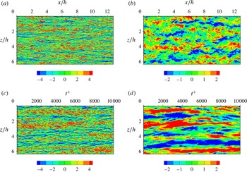
direction (Toh & Itano Reference Toh and Itano2005). In figure 15, the t–z contours of
 $u^{2D}$
for the MSU are compared with the x–z contours of
 $u$
for the LSD. Two wall-normal locations (
 $y^{+}=15$
and
 $y/h=0.5$
) are examined. The similarity between
 $u$
and
 $u^{2D}$
is convincing in the inner region. In this figure, we also see the good correspondence in locations between the dense clustering patterns of near-wall streaks and the LSMs. The former are thus footprints of the LSMs (see Abe et al.
Reference Abe, Kawamura and Choi2004b
; Hutchins & Marusic Reference Hutchins and Marusic2007a
,Reference Hutchins and Marusic
b
). We stress that the dense clustering patterns become more energetic for the MSU than for the LSD. Figure 16(a) shows the spanwise spectra of
 $u$
,
 $v$
, and
 $w$
normalized by
 $U_{\unicode[STIX]{x1D70F}}^{2}$
and
 $\unicode[STIX]{x1D708}/U_{\unicode[STIX]{x1D70F}}$
for
 $h^{+}=1020$
at
 $y^{+}=15$
for the MSU and LSD/VLSD. The high-wavenumber behaviour is nearly identical between the MSU and LSD/VLSD, while the energy at low and intermediate wavenumbers in the
 $u$
and
 $w$
spectra are increased and decreased, respectively, for the MSU. In particular, the energy at low and intermediate wavenumbers (i.e.
 $k_{z}h=5\sim 50$
) in the
 $u$
spectra is approximately 30 % larger for the MSU than for the LSD (see figure 16
b). Also, the energy in the
 $u$
spectra for the MSU is more enhanced at very low wavenumbers (i.e.
 $k_{z}h<5$
) than at low and intermediate wavenumbers (i.e.
 $k_{z}h=5\sim 50$
), where the peak is invariably observed at
 $k_{z}h\approx 2$
, or equivalently,
 $\unicode[STIX]{x1D706}_{z}/h\approx 3$
across the channel (figure 16
d). In the LSD, the latter spectral peak is exclusively observed in the core region (figure 16
c). This indicates that the superimposition of the LSMs as a low-wavenumber mean shift onto the near-wall region (see Hutchins & Marusic Reference Hutchins and Marusic2007b
) is significantly enhanced for the MSU. Note that the large-scale spanwise meandering (Hutchins & Marusic Reference Hutchins and Marusic2007a
,Reference Hutchins and Marusic
b
) and waviness of the large-scale structures (Flores & Jiménez Reference Flores and Jiménez2010) in the logarithmic region are not observed in the MSU (see figure 10
f). The latter behaviour is essentially associated with the decreased logarithmic dependence of
 $\overline{ww}$
shown in figure 3(f).
Comparison between x–z contours of
 $u$
for the LSD (
 $L_{x}=12.8h$
) (a,b) and t–z contours of
 $u^{2D}$
for the MSU (c,d) for
 $h^{+}=1020$
. The data at
 $y^{+}=15$
are plotted in (a,c), whereas those at
 $y/h=0.5$
are shown in (b,d). In (a,b), the instantaneous
 $u$
data in the LSD have been plotted at the two
 $y$
locations in the x–z plane. In (c,d), the time evolution data of
 $u^{2D}$
, defined in (3.18), in the MSU have been plotted at the two
 $y$
locations as a function of the spanwise location.

Normalized one-dimensional spanwise spectra of velocity fluctuations: (a)
 $\unicode[STIX]{x1D719}_{uu}(k_{z})/U_{\unicode[STIX]{x1D70F}}\unicode[STIX]{x1D708}$
,
 $\unicode[STIX]{x1D719}_{vv}(k_{z})/U_{\unicode[STIX]{x1D70F}}\unicode[STIX]{x1D708}$
,
 $\unicode[STIX]{x1D719}_{ww}(k_{z})/U_{\unicode[STIX]{x1D70F}}\unicode[STIX]{x1D708}$
at
 $y^{+}=15$
; (b)
 $\unicode[STIX]{x1D719}_{uu}(k_{z})/U_{\unicode[STIX]{x1D70F}}^{2}h$
at
 $y^{+}=15$
and
 $y/h=0.5$
; (c)
 $\unicode[STIX]{x1D719}_{uu}(k_{z})/U_{\unicode[STIX]{x1D70F}}^{2}h$
for the LSD at
 $y^{+}=5$
, 61 and
 $y/h=0.2$
, 0.5, 0.8; (d)
 $\unicode[STIX]{x1D719}_{uu}(k_{z})/U_{\unicode[STIX]{x1D70F}}^{2}h$
for the MSU at
 $y^{+}=5$
, 61 and
 $y/h=0.2$
, 0.5, 0.8. In (a,b), the spectra for the MSU have been compared with those for the LSD. In (c,d), the spectra have been plotted in inner scales to highlight the low-wavenumber behaviour. In (a), – – – – denotes the DNS data of del Álamo et al. (Reference del Álamo, Jiménez, Zandonade and Moser2004) for
 $h^{+}=934$
with the VLSD (
 $L_{x}=8\unicode[STIX]{x03C0}h$
).

Time variation of the large-scale structures in the MSU for
 $h^{+}=1020$
: (a)
 $t^{+}=0$
; (b)
 $t^{+}=600$
; (c)
 $t^{+}=1200$
; (d)
 $t^{+}=1800$
: red,
 $u^{+}>1.5$
; blue,
 $u^{+}<-1.5$
. Spanwise scales below 0.5
 $h$
are filtered out with the use of a spectral sharp cutoff filter. The visualization domain size shown here is the whole computational domain for the MSU (i.e.
 $0.4h\times 2h\times 6.4h$
in the
 $x$
,
 $y$
and
 $z$
directions, respectively).

Figure 17 demonstrates how the large-scale structures in the MSU for
 $h^{+}=1020$
evolve in time, where structures with a spanwise scale larger than 0.5
 $h$
are illustrated with the use of a sharp cut filter. Indeed, large-scale structures become increasingly larger with increasing distance from the wall. The positive and negative large-scale
 $u$
structures with a spanwise spacing of approximately 0.8
 $h$
are observed below the log region (
 $y/h\leqslant 0.2$
), whereas those with a spanwise spacing of 1.6
 $h$
dominate in the outer region (
 $y/h>0.2$
), consistent with the peak wavelengths of the spanwise premultiplied
 $u$
spectra (figure 12
a). Note that we also see the large-scale structures spanning the channel half-width with a spanwise spacing approximately 3
 $h$
for the MSU, as discussed below. Near the centreline, large-scale structures originating from one wall interact with those from the other wall, which is reminiscent of the large flow recirculation observed by Toh & Itano (Reference Toh and Itano2005) at low Reynolds numbers. There is however a discernible difference between the present MSU and that of Toh & Itano (Reference Toh and Itano2005) due to the closer approach towards two-dimensionality in the present MSU (see figure 2
d). Consequently, the large-scale structures in the present MSU are present for a long period of time, as opposed to those in Toh & Itano (Reference Toh and Itano2005) (see also the persistent outer spectral peak for the MSU shown in figure 14
b). This is most likely due to the lack of nonlinear evolution of the large-scale structures in the present MSU. Figure 17 underlines that antisymmetric pairs (with respect to centreline) of large-scale structures, with a spanwise spacing of approximately 3
 $h$
, dominate in the MSU. The latter spanwise spacing corresponds to the peak wavelength observed in the spanwise
 $u$
spectra across the channel (figure 16
d). Because of the two-dimensionality of the large-scale structures (in the MSU), which carry a large amount of the turbulent kinetic energy, we have associated this peak wavelength with that in the transient growth simulation. Indeed, the peak wavelength in the present MSU (approximately 3
 $h$
) is very close to the optimal spanwise wavelength of 3
 $h$
reported by del Álamo & Jiménez (Reference del Álamo and Jiménez2006). Pujals et al. (Reference Pujals, Manuel Garcia-Villalba, Cossu and Depardon2009) also reported an optimal spanwise spacing of 4
 $h$
for the optimal transient growth of perturbations in a turbulent channel flow. Also, to provide statistical evidence regarding the antisymmetric pairs of large-scale structures, wall-normal two-point correlations, defined such that
 $$\begin{eqnarray}\displaystyle & \displaystyle R_{\unicode[STIX]{x1D6FC}\unicode[STIX]{x1D6FC}}(y_{r},y)={\displaystyle \frac{\overline{\unicode[STIX]{x1D6FC}(y_{r})\unicode[STIX]{x1D6FC}(y)}}{\overline{\unicode[STIX]{x1D6FC}(y_{r})\unicode[STIX]{x1D6FC}(y_{r})}}}, & \displaystyle\end{eqnarray}$$
where
 $y_{r}$
is a reference
 $y$
location and
 $\unicode[STIX]{x1D6FC}\equiv u$
,
 $v$
,
 $w$
or
 $p$
, have been examined. Figure 18 exhibits the anomalous behaviour for the
 $u$
component of the MSU, which supports the antisymmetric pattern of large-scale structures observed in figure 17. Note that for this quantity, the averaging is based on a time period
 $t^{+}\approx 1300$
and 1800, for the LSD and MSU, respectively. The sampling time period for the MSU corresponds to the time period, shown in figure 17, related to the evolution of the large-scale structures. The present sampling time period is approximately 6–8 times larger than that used by Kim & Hussain (Reference Kim and Hussain1993) in the analysis of the space–time correlations for
 $h^{+}=180$
; the longer sampling yields a better convergence for correlations at large separations. While the
 $u$
correlations for the LSD tend to approach zero at large separations, those for the MSU indeed exhibit asymmetric patterns with respect to the centreline (see figure 18). The antisymmetric pattern is also identical with the most amplified outer mode of a transient growth of perturbations (see del Álamo & Jiménez Reference del Álamo and Jiménez2006; Pujals et al.
Reference Pujals, Manuel Garcia-Villalba, Cossu and Depardon2009). In this context, Butler & Farrell (Reference Butler and Farrell1992) noted in their analysis of laminar transient growth that the parabolic shape of the mean flow leads to the growth of
 $u$
in antisymmetric pairs. Indeed, when
 $h^{+}$
reaches 1020 and the two-dimensionality is established approximately for the MSU, there is an increase in
 $\overline{U}^{+}$
(figure 1
a) and the distribution of
 $\overline{U}^{+}$
is closer to the parabolic profile (figure 1
b). The present results underline that the most energetic mode in the transient growth of perturbations is most likely the origin of the global
 $u$
mode in a turbulent channel flow.
Wall-normal two-point correlations for
 $h^{+}=1020$
: (a)
 $R_{uu}(y_{r},y)$
; (b)
 $R_{vv}(y_{r},y)$
; (c)
 $R_{ww}(y_{r},y)$
; (d)
 $R_{pp}(y_{r},y)$
. In this figure, the averaging is based on a time period
 $t^{+}\approx 1300$
and 1800, for the LSD and MSU, respectively. The locations of
 $y_{r}$
are
 $y/h=0$
, 0.2, 0.5 and 1. The data at
 $y_{r}=0$
have been obtained at the first grid point.

Contours in the
 $y$
–
 $z$
plane of instantaneous total, slow rapid pressure for
 $h^{+}=1020$
: (a,b)
 $p$
; (c,d)
 $p_{s}$
; (e,f)
 $p_{r}$
. (a,c,e) correspond to the LSD (
 $L_{x}=12.8h$
), while (b,d,f) are for the MSU (
 ${L_{x}}^{+}\approx 400$
). The visualized instantaneous field is the same as in figure 10.

3.4 Pressure fluctuations
In this subsection, we examine the reason why the wall-attached pressure fluctuations are attenuated in the MSU. As in Jiménez & Hoyas (Reference Jiménez and Hoyas2008), we adopt the pressure splitting method, i.e. the slow and rapid pressure (
 $p_{s}$
,
 $p_{r}$
) obtained by solving Poisson’s equation, viz.
 $$\begin{eqnarray}\displaystyle & \displaystyle \unicode[STIX]{x1D6FB}^{2}p_{s}^{+}=-{\displaystyle \frac{\unicode[STIX]{x2202}u_{i}^{+}}{\unicode[STIX]{x2202}x_{j}^{\#}}}{\displaystyle \frac{\unicode[STIX]{x2202}u_{j}^{+}}{\unicode[STIX]{x2202}x_{i}^{\#}}} & \displaystyle\end{eqnarray}$$
and
 $$\begin{eqnarray}\displaystyle & \displaystyle \unicode[STIX]{x1D6FB}^{2}p_{r}^{+}=-2{\displaystyle \frac{\unicode[STIX]{x2202}v^{+}}{\unicode[STIX]{x2202}x^{\#}}}{\displaystyle \frac{\unicode[STIX]{x2202}\overline{U}^{+}}{\unicode[STIX]{x2202}y^{\#}}} & \displaystyle\end{eqnarray}$$
(see also Abe, Matsuo & Kawamura Reference Abe, Matsuo, Kawamura, Humphrey, Gatski, Eaton, Friedrich, Kasagi and Leschziner2005). Note that the superscript # denotes normalization by the channel half-width. The boundary conditions at the wall are
 $\unicode[STIX]{x2202}p_{s}^{+}/\unicode[STIX]{x2202}y^{\#}=(1/h^{+})(\unicode[STIX]{x2202}^{2}v^{+}/\unicode[STIX]{x2202}y^{\#2})$
and
 $\unicode[STIX]{x2202}p_{r}^{+}/\unicode[STIX]{x2202}y^{\#}=0$
; the Stokes pressure is included in the slow pressure. The rapid and slow pressure are sometimes referred to as the linear and nonlinear pressure, respectively, (see Kim Reference Kim1989) because the Poisson equations for the slow and rapid pressure have nonlinear–nonlinear (the term on the right-hand side of (3.20)) and linear–nonlinear (the term on the right-hand side of (3.21)) interactions, respectively. Here, we use 50 and 600 time consecutive datasets for the LSD and MSU, respectively, with a time interval of
 $\unicode[STIX]{x0394}t^{+}\approx 3$
for
 $h^{+}=1020$
. In the following statistics, the time averaging has been performed with these time consecutive datasets, viz.
 $t^{+}\approx 150$
and 1800 for the LSD and MSU, respectively.
Figure 19 shows the instantaneous contours in the y–z plane of the total, rapid and slow pressure for the LSD and MSU for
 $h^{+}=1020$
. In contrast to the x–y plane, the instantaneous contours in the y–z plane show a noticeable difference between
 $w$
and
 $p$
(see figures 10
e and 19
a). This is essentially associated with a difference between the three-dimensional shear layers and the wall-attached structures of the pressure (see also the different behaviours in the wall-normal two-point correlations of
 $w$
and
 $p$
shown in figure 18
c,d). The pressure splitting decomposes the shear-layer structures and tall ones. The slow pressure
 $p_{s}$
for the LSD (figure 19
c) shows rounded structures in the y–z plane, which are the cross-sections of streamwise sloping structures (see figure 4
c). On the other hand, the rapid pressure
 $p_{r}$
for the LSD (figure 19
e) shows tall global structures, which is most likely a consequence of the behaviour that high momentum large-scale structures impact on low momentum large-scale ones (see figure 4
a). When the streamwise domain
 $L_{x}$
is reduced to the size of MSU, these structures become indeed smaller (see figure 19) and exhibit localized structures. In particular, there is a significantly reduced magnitude of the rapid pressure, which is essentially associated with the weakened linear–nonlinear interaction in the Poisson equation (viz. the term on the right-hand side of (3.21)).
Distributions of mean-square pressure fluctuations (
 $\overline{pp}/\unicode[STIX]{x1D70F}_{w}^{2}$
,
 $\overline{p_{s}p_{s}}/\unicode[STIX]{x1D70F}_{w}^{2}$
,
 $\overline{p_{r}p_{r}}/\unicode[STIX]{x1D70F}_{w}^{2}$
) for
 $h^{+}=1020$
: (a) LSD (
 $L_{x}=12.8h$
); (b) MSU (
 ${L_{x}}^{+}\approx 400$
). In each figure, the relation of (3.8) is plotted as the two-dotted line.

To provide the corresponding statistical evidence, figure 20 shows the mean square values for both the MSU and LSD. Indeed, the magnitudes of
 $p_{s}$
and
 $p_{r}$
are reduced in the MSU where
 $p_{s}$
is the sole contributor to the pressure fluctuations away from the wall, consistent with the result in the instantaneous fields (figure 19). Figure 21(a,b) shows the streamwise and spanwise power spectra of the total, slow rapid pressure for
 $h^{+}=1020$
in the outer region (
 $y/h=0.5$
) of the LSD and MSU. The streamwise spectra for the MSU agree reasonably well with those for the LSD up to their smallest non-zero wavenumbers, whilst the spanwise spectra for the MSU show a smaller magnitude at low wavenumbers than for the LSD. Indeed, there is a better spectral similarity between the total and slow pressure for the MSU in the outer region than for the LSD (see figure 21
a,b), consistent with the result in the mean-square values (see figure 20). This result indicates that the spectral similarity between
 $w$
and
 $p$
in the outer region observed in figure 8 is intrinsically associated with the slow pressure. We also note that there is a significant decrease in power at low wavenumbers in the spanwise
 $p_{r}$
spectra of the MSU (see figure 21
b). Also, a local peak appearing in the streamwise
 $p_{r}$
spectra (not in the streamwise
 $p_{s}$
spectra) at
 $k_{x}h=2\sim 3$
(i.e.
 $\unicode[STIX]{x1D706}_{x}/h=2\sim 3$
) across the channel for the LSD is not reproduced for the MSU (see figure 21
c,d). These behaviours are consistent with the weakened structures for the MSU observed in figures 4(b) and 19(b) and essentially associated with the significantly decreased logarithmic dependence of
 $\overline{pp}/\unicode[STIX]{x1D70F}_{w}^{2}$
(figure 7
d). We have also examined the pressure strain terms for the total
 $\unicode[STIX]{x1D719}_{ij}^{t}$
, slow
 $\unicode[STIX]{x1D719}_{ij}^{s}$
, rapid
 $\unicode[STIX]{x1D719}_{ij}^{r}$
pressure (figure 22) to gain further insight into the weakened redistribution in the MSU (see figure 9
e). Indeed, the magnitudes of
 $\unicode[STIX]{x1D719}_{11}^{r}$
and
 $\unicode[STIX]{x1D719}_{33}^{r}$
are attenuated significantly in the MSU, consistent with the weakened structures (figure 10
f). Given that
 $\unicode[STIX]{x1D719}_{33}^{r}$
is the major contributor to
 $\unicode[STIX]{x1D719}_{33}^{t}$
away from the wall, the reduced
 $\unicode[STIX]{x1D719}_{33}^{r}$
in the MSU is essentially associated with the reduced magnitude of
 $\overline{ww}/U_{\unicode[STIX]{x1D70F}}^{2}$
(figure 7
b). The reason for the reduced energy redistribution in the MSU is therefore essentially associated with the impaired global nature of the pressure largely resulting from the reduced linear–nonlinear interaction in the Poisson equation (i.e. the rapid pressure).
Streamwise and spanwise power spectra of the total, slow and rapid pressure normalized by
 $\unicode[STIX]{x1D70F}_{w}^{2}$
and
 $h$
,
 $\unicode[STIX]{x1D719}_{pp}(k_{x})/\unicode[STIX]{x1D70F}_{w}^{2}h$
and
 $\unicode[STIX]{x1D719}_{pp}(k_{z})/\unicode[STIX]{x1D70F}_{w}^{2}h$
, for
 $h^{+}=1020$
: (a)
 $\unicode[STIX]{x1D719}_{pp}(k_{x})/\unicode[STIX]{x1D70F}_{w}^{2}h$
at
 $y/h=0.5$
; (b)
 $\unicode[STIX]{x1D719}_{pp}(k_{z})/\unicode[STIX]{x1D70F}_{w}^{2}h$
at
 $y/h=0.5$
; (c)
 $\unicode[STIX]{x1D719}_{pp}(k_{x})/\unicode[STIX]{x1D70F}_{w}^{2}h$
for the slow pressure; (d)
 $\unicode[STIX]{x1D719}_{pp}(k_{x})/\unicode[STIX]{x1D70F}_{w}^{2}h$
for the rapid pressure. In (c,d), the
 $y$
stations of the spectra plotted are
 $y/h=0$
, 0.2, 0.5, 0.7 and 1.

Distributions of the pressure strain terms for the total, slow and rapid pressure normalized by wall units for
 $h^{+}=1020$
: (a)
 $\unicode[STIX]{x1D719}_{11}^{t}$
,
 $\unicode[STIX]{x1D719}_{11}^{s}$
,
 $\unicode[STIX]{x1D719}_{11}^{r}$
; (b)
 $\unicode[STIX]{x1D719}_{22}^{t}$
,
 $\unicode[STIX]{x1D719}_{22}^{s}$
,
 $\unicode[STIX]{x1D719}_{22}^{r}$
; (c)
 $\unicode[STIX]{x1D719}_{33}^{t}$
,
 $\unicode[STIX]{x1D719}_{33}^{s}$
,
 $\unicode[STIX]{x1D719}_{33}^{r}$
.

4 Conclusions
In the present study, we have examined the MSU (i.e.
 ${L_{x}}^{+}\approx 400$
) in a turbulent channel flow with the use of DNS datasets at larger
 $h^{+}$
than in the original work (Toh & Itano Reference Toh and Itano2005). Two values of the Kármán number (
 $h^{+}=395$
and 1020) are used for the MSU. DNS datasets (
 $h^{+}=180$
to 1020) obtained with the LSD (i.e.
 $L_{x}=12.8h$
) are also compared with those obtained with VLSDs in the literature. Particular attention has been given to whether the spanwise organization of the large-scale structures may be represented properly in this simplified system for a sufficiently large
 $h^{+}$
and how these structures are associated with the mean streamwise velocity
 $\overline{U}$
. We have also discussed the importance of two features of the large-scale structures, i.e. their streamwise inclination and spanwise meandering, by comparing the results for the MSU with those obtained with a large
 $L_{x}$
domain; the streamwise domain for the MSU becomes increasing smaller, in terms of
 $L_{x}/h$
, as
 $h^{+}$
increases. The main conclusions are as follows.
In the MSU, the mean velocity
 $\overline{U}$
and Reynolds shear stress
 $\overline{uv}$
are captured satisfactorily. One discernible difference, relative to the LSD, is that a larger magnitude of the mean velocity arises in the outer region of the MSU as
 $h^{+}$
increases. This is due to an approach towards two-dimensionality of the large-scale structures, which results in an impaired global nature of the pressure and attenuates the energy redistribution. As
 $h^{+}$
increases, the streamwise Reynolds stress
 $\overline{uu}$
becomes increasingly energetic whereas the spanwise Reynolds stress
 $\overline{ww}$
decreases significantly. The latter exhibits a clearer logarithmic dependence than for the LSD (see figure 3
f) due to a reduction in spanwise large scales, associated with
 $w$
, for the MSU (see figures 4
c and 10
f). The present result corroborates the finding by Jiménez & Hoyas (Reference Jiménez and Hoyas2008) that most of the departure from the logarithmic behaviour of
 $\overline{uu}$
is due to the very long and wide eddies in
 $u$
. Given that the most energetic spanwise scales for the MSU vary linearly with increasing distance from the wall (see figure 12
c), the well-established logarithmic dependence of
 $\overline{ww}/U_{\unicode[STIX]{x1D70F}}^{2}$
in the MSU is intrinsically associated with the attached eddy hypothesis of Townsend (Reference Townsend1976).
After clarifying the Reynolds-number dependence in the MSU, the effect of varying
 $L_{x}$
, from 0.4
 $h$
to 12.8
 $h$
, has been examined both statistically and instantaneously for
 $h^{+}=1020$
. There is a significant effect on the inactive motion, viz.
 $\overline{ww}$
and
 $\overline{pp}$
, when
 $L_{x}<2\unicode[STIX]{x03C0}h$
. The latter criterion is identical with the finding of Lozano-Durán & Jiménez (Reference Lozano-Durán and Jiménez2014) and intrinsically associated with the streamwise extent of the LSMs, with a length in the range
 $2\sim 4h$
. There is a close similarity between the streamwise
 $w$
and
 $p$
spectra, whereas the spanwise
 $w$
spectra show more prominent peaks than the spanwise
 $p$
spectra. Indeed,
 $w$
displays spanwise large-scale structures, while
 $p$
exhibits smaller scale structures than
 $w$
. This behaviour is associated with a wider
 $y$
range of the logarithmic dependence of
 $\overline{pp}/\unicode[STIX]{x1D70F}_{w}^{2}$
than that of
 $\overline{ww}/U_{\unicode[STIX]{x1D70F}}^{2}$
, consistent with the finding of Jiménez & Hoyas (Reference Jiménez and Hoyas2008) that because of the lack of very large scales, the pressure fluctuations away from the wall scale very well with
 $\unicode[STIX]{x1D70C}U_{\unicode[STIX]{x1D70F}}^{2}$
(or equivalently,
 $\unicode[STIX]{x1D70F}_{w}$
). We have also provided statistical evidence regarding the similarity between
 $\overline{pp}$
and
 $\overline{\unicode[STIX]{x1D700}}$
. Whilst the mean velocity log law appears to hold for
 $h^{+}\geqslant 5000$
, small-scale quantities and pressure fluctuations are less affected by viscosity and exhibit an outer-layer similarity at a smaller
 $h^{+}$
than that at which the mean velocity log law is established. On the other hand, the spanwise
 $u$
organization is essentially unaffected. Three most energetic spanwise scales are obtained for
 $u$
, viz.
 ${\unicode[STIX]{x1D706}_{z}}^{+}\approx 100$
,
 $\unicode[STIX]{x1D706}_{z}/h=0.8\sim 0.9$
and
 $\unicode[STIX]{x1D706}_{z}/h=1.3\sim 1.6$
in the near-wall, logarithmic and outer regions, respectively. There is also a linear increase of spanwise scale in the range
 $40\leqslant y^{+}\leqslant 80$
. We note that the large-scale structures in the MSU are more energized in the outer region (
 $y/h>0.2$
) due to a reduced turbulent diffusion; one extra spectral peak is invariably observed at
 $k_{z}h\approx 2$
, viz.
 $\unicode[STIX]{x1D706}_{z}\approx 3h$
, across the channel in the MSU, identical with the most amplified outer mode of the optimal transient growth of perturbations (del Álamo & Jiménez Reference del Álamo and Jiménez2006). This is a consequence of the tight coupling between neighbouring structures. In particular, there is a close interaction between large-scale structures originating from one wall and those from the other wall in the MSU. The present results underline that when the two-dimensional behaviour is approached at a sufficiently large
 $h^{+}$
, the minimal streamwise unit convincingly identifies the spanwise
 $u$
pattern observed in the outer mode of a transient growth of perturbations. This latter mode is likely to be at the origin of the global
 $u$
mode obtained with the LSD/VLSD.
Attention has also been given to the pressure fluctuations
 $p$
with the use of the pressure splitting method (viz. the rapid and slow pressure). In the MSU, the rapid pressure is reduced significantly away from the wall region owing to the weakened linear–nonlinear interaction in Poisson’s equation, which reduces the energy redistribution to
 $\overline{ww}$
. The slow pressure is thus the sole contributor to
 $p$
in the outer region of the MSU, where localized structures dominate. The global nature of the pressure is indeed lacking in the MSU at large
 $h^{+}$
due to the reduced linear–nonlinear interaction.
The present study underlines that while the approach towards two-dimensionality of the large-scale structures may be an ‘artefact’ of the domain size used for the MSU, this simplified system reproduces the spanwise organization of the large-scale structures in the log region correctly even at a sufficiently large
 $h^{+}$
, and the well-established logarithmic mean velocity distribution (see figure 1
a). On the other hand, the large-scale structures in the outer region are more energetic for the MSU than for the LSD/VLSD. By concentrating on the MSU, our understanding of the importance of the streamwise inclination and spanwise meandering of the large-scale structures has been improved. When the two-dimensionality of the large-scale structures is approached in the outer region of the MSU,
 $\overline{uu}$
and
 $\overline{ww}$
are more and less energized. This is associated with the reduced energy redistribution, owing to the impaired global nature of the pressure, and an improved logarithmic dependence of
 $\overline{ww}/U_{\unicode[STIX]{x1D70F}}^{2}$
due to the reduced spanwise large scales. These indirect inferences regarding the importance of two features of the large-scale structures are major outcomes of the present MSU study, which further highlight the advantages offered by the minimal flow unit ‘numerical experiment’ (Jiménez & Moin Reference Jiménez and Moin1991).
Acknowledgements
Computations performed on the JAXA (Japan Aerospace Exploration Agency) Supercomputer System are gratefully acknowledged. This study has been triggered by discussion with Professor H. Kawamura, the advisor of the first author during his PhD work. H.A. is grateful to Professor T. Itano and Dr Y. Matsuo for earlier collaborations and to Professor A. Yoshizawa for fruitful discussions during the course of this work. H.A. also acknowledges important comments and suggestions made by the referees on the first and second versions of this manuscript.