1 Introduction
For massive enough stars, nuclear fusion is able to produce elements heavier than carbon and oxygen up to the production of the most stable nucleus, iron  ${}^{56}$Fe. At this point the core of the star collapses and the outer layers fall onto the core, triggering a supernova explosion leaving behind a compact remnant which can either be a black hole or a neutron star. In this paper, we focus on strongly magnetized and fast rotating neutron stars. These compact objects are believed to be among the most efficient accelerators in the universe, producing ultra-relativistic particles (electrons, positrons, protons and maybe ions). In its simplest description, a neutron star is described thanks to only a few parameters, namely
(a) the inclination angle or obliquity
 $\chi$ which represent the angle between the rotation axis and magnetic axis;
(b) the angular speed
$\varOmega$ which defines the light cylinder radius $r_{L}=c/\varOmega$, the distance at which an object in co-rotation with the star reaches the speed of light $c$;(c) the radius of the neutron star
$R$;(d) the magnetic field strength
$B$ at the surface on the equator.


The extreme magnetic fields of these remnant stars range from  $B\simeq 10^5$ to
 $B\simeq 10^{10}\ \text {T}$, which, coupled with an angular speed between
 $\varOmega \simeq 1000\ \text {rad}\ \text {s}^{-1}$ and
 $\varOmega \simeq 0.1\ \text {rad}\ \text {s}^{-1}$, generates an intense electric field,
 $E$, of the order
 $\varOmega BR \approx 10^{12}$ V m
 $^{-1}$, accelerating particles around the neutron star to ultra-relativistic Lorentz factors. In our applications, the neutron star mass
 $M$ is irrelevant because the gravitational force exerted on charged particles
 $F_g$ is negligible compared to the Lorentz force
 $F_L$. Indeed, both forces have a typical intensity of
 $F_g = G ({M m_p}/{R^2} \simeq 3.17\times 10^{-15}\ \text {N}$ for a proton at the surface of the neutron star compared to
 $F_L = q E = q \varOmega R B \simeq 5.01\times 10^{-7}\ \text {N}$. The ratio of these forces is
 \begin{equation} \frac{F_g}{F_L} = \frac{G M m_p}{R^2 q E} = 6.33 \times 10^{-9} \ll 1 , \end{equation}
so the electromagnetic force is  ${\sim }10^{8}$ times stronger than the gravitational force for protons and a factor
 $m_p/m_e$ larger for electrons and positrons.
Most numerical simulations of neutron star magnetospheres use the Boris (Reference Boris1970) algorithm or, better, the Vay (Reference Vay2008) algorithm. However,these algorithms are not well suited for ultra-strong electromagnetic fields, forcing some authors to lower the true field strengths to unrealistically low values in simulations. Although a scaling is sometimes applied to get more realistic results, such scaling cannot be straightforwardly extrapolated for instance when radiation reaction is included because of the nonlinearities introduced by radiative feedback (Vranic et al. Reference Vranic, Martins, Fonseca and Silva2016). Moreover, Lorentz factors reached by the particles near pulsars hardly exceed  $\gamma =10^4$ with those algorithms, see for instance Brambilla et al. (Reference Brambilla, Kalapotharakos, Timokhin, Harding and Kazanas2018), Philippov & Spitkovsky (Reference Philippov and Spitkovsky2014), Guépin, Cerutti & Kotera (Reference Guépin, Cerutti and Kotera2019) and Kalapotharakos et al. (Reference Kalapotharakos, Brambilla, Timokhin, Harding and Kazanas2018).
Several attempts have been proposed to faithfully follow particles in relativistic regimes, trying to conserve energy and momentum. In this spirit, Zenitani & Umeda (Reference Zenitani and Umeda2018) improved the Boris (Reference Boris1970) particle pusher by computing the exact analytical rotation in the magnetic field and getting better accuracy. The Boris algorithm is, however, popular because of its simplicity and accuracy. Moreover, its stability property takes its root in its phase space volume preserving properties, as discussed by Qin et al. (Reference Qin, Zhang, Xiao, Liu, Sun and Tang2013). Umeda (Reference Umeda2018) also improved the Boris algorithm by employing a three stage step. Relativistic simulations are even more stringent about numerical error accumulation and volume preserving schemes are highly recommended, as pointed out by Zhang et al. (Reference Zhang, Liu, Qin, Wang, He and Sun2015).
Efficient particle pushers in ultra-strong electromagnetic fields are fundamental to simulating the neutron star electrodynamics. For a comprehensive comparison of relativistic particle integrators, see the extensive work done by Ripperda et al. (Reference Ripperda, Bacchini, Teunissen, Xia, Porth, Sironi, Lapenta and Keppens2018). They carefully compared the merit of the standard Boris algorithm (Boris Reference Boris1970), the Vay (Reference Vay2008) implicit scheme in space velocity, the Higuera & Cary (Reference Higuera and Cary2017) second-order method and the implicit midpoint method described in Lapenta & Markidis (Reference Lapenta and Markidis2011). This leapfrog scheme already appeared in Verboncoeur (Reference Verboncoeur2005). A fully implicit update in space and velocity parameters for relativistic particle integrators relying on the Vay (Reference Vay2008) velocity advance has been explored by Pétri (Reference Pétri2017). There, it has been shown that catching properly and accurately the simple electric drift motion in an ultra-relativistic regime remains extremely difficult to achieve. Unfortunately, neutron star magnetospheres are common places for such relativistic drift velocities. It is therefore compulsory to design efficient and accurate numerical schemes to faithfully follow these trajectories. It represents a crucial step towards realistic particle acceleration and radiation in ultra-strong electromagnetic fields. Some tests of particle acceleration in a plane electromagnetic wave using standard pushers and reported by Arefiev et al. (Reference Arefiev, Cochran, Schumacher, Robinson and Chen2015) showed severe limitations in the accuracy already for modest field strengths with strength parameter  $a\approx 20$ (see (1.2)).
The limitation arises from the huge span in time scales, from the gyroperiod frequency  $\omega _B=qB/m$ to the stellar rotation frequency
 $\varOmega$ and synthesized by the strength parameter
 \begin{equation} a = \frac{\omega_B}{\varOmega} = \frac{qB}{m\varOmega}\simeq10^{10}, \end{equation}
for a proton near a millisecond pulsar ( $\varOmega =10^{3}\ \text {rad}\ \text {s}^{-1}$ and
 $B=10^{5}\ \text {T}$), the situation being worst for electron/positron pairs. This ratio corresponds to the number of gyrations made by a particle during the time scale of evolution of the electromagnetic field due to the stellar rotation. It shows that the difference in time scales makes it almost impossible to compute the trajectory of particles in a reasonable amount of time, since billions of time steps are needed on the pulsar period time scale. To tackle this issue, our aim is to propose a new technique based on analytical solutions of the Lorentz force equation in constant and ultra-strong electromagnetic fields with an acceptable computational time and most importantly avoiding a necessary scaling, allowing particles to reach high Lorentz factors with realistic fields.
Neutron stars are known to act as unipolar inductors, generating huge electric potential drops between the poles and the equator, of the order
 \begin{equation} {\rm \Delta} \phi = \varOmega B R^2 \approx 10^{16}\ \textrm{V}. \end{equation}
As a consequence, they expel electrons, maybe protons and ions, filling the magnetosphere with charged particles. Typical Lorentz factors for electrons in this static field are therefore
 \begin{equation} \gamma = \frac{e {\rm \Delta}\phi}{m_e c^2} \approx 10^{10}. \end{equation}
If the particle injection rate is high enough, this plasma will screen the electric field, drastically mitigating the potential drop  ${\rm \Delta} \phi$ and the acceleration efficiency. Resistive (Li, Spitkovsky & Tchekhovskoy Reference Li, Spitkovsky and Tchekhovskoy2012) and particle in cell (PIC) simulations (Cerutti et al. Reference Cerutti, Philippov, Parfrey and Spitkovsky2015) showed that, indeed, only a small fraction of the full potential is available. However, for low particle injection rates, the plasma is unable to screen the electric field and the full potential drop develops. The magnetosphere is then almost empty and known as an electrosphere (Krause-Polstorff & Michel Reference Krause-Polstorff and Michel1985; Pétri, Heyvaerts & Bonazzola Reference Pétri, Heyvaerts and Bonazzola2002). Such electrospheres are the subject of the present paper. They represent inactive pulsars able to accelerate particles to ultra-relativistic speeds. We aim at accurately quantifying the final Lorentz factor reached by the outflowing plasma in this large amplitude low frequency electromagnetic wave. Similar studies have been performed by Michel & Li (Reference Michel and Li1999) staying, however, on a more analytical side.
The outline of the paper is as follows. First, in § 2, we briefly recall the principle of the algorithm. Next, in § 3, we show some results obtained in fields where an analytical solution is known before discussing the convergence to the exact solution in § 4. Results of the simulations near pulsars are presented in § 5. Some conclusions are drawn in § 6.
2 Outline of the numerical algorithm
In this section we summarize the scheme of our algorithm. A more complete and careful description can be found in Pétri (Reference Pétri2020c) with a more comprehensive introduction pointing to appropriate references. The code is based on successive exact analytical solutions for the trajectory of a relativistic particle in a constant but otherwise arbitrary electromagnetic field  $(\boldsymbol {E}, \boldsymbol {B})$. Switching to a frame where
 $\boldsymbol {E}$ and
 $\boldsymbol {B}$ are parallel and aligned with the
 $\boldsymbol {e}_z$ axis, integration of the Lorentz force in a Cartesian coordinate system
 $(\boldsymbol {e}_x, \boldsymbol {e}_y, \boldsymbol {e}_z)$ leads to the 4-velocity given by
 \begin{gather} u^0 = \gamma_0 c [\cosh (\omega_E \tau) + \beta_0^z \sinh (\omega_E \tau)] \end{gather}
 \begin{gather}u^1 = \gamma_0 c [\beta_0^x \cos(\omega_B \tau) + \beta_0^y \sin (\omega_B \tau)] \end{gather}
 \begin{gather}u^2 = \gamma_0 c [-\beta_0^x \sin(\omega_B \tau) + \beta_0^y \cos (\omega_B \tau)] \end{gather}
 \begin{gather}u^3 = \gamma_0 c [\sinh (\omega_E \tau) + \beta_0^z \cosh (\omega_E \tau)] \end{gather}
and to the 4-position
 \begin{gather} c(t-t_0) = \frac{\gamma_0 c}{\omega_E} [\sinh (\omega_E \tau) + \beta_0^z \cosh (\omega_E \tau) - \beta_0^z] \end{gather}
 \begin{gather}x-x_0 = \frac{\gamma_0 c}{\omega_B} [\beta_0^x \sin(\omega_B \tau) - \beta_0^y \cos (\omega_B \tau) +\beta_0^y] \end{gather}
 \begin{gather}y-y_0 = \frac{\gamma_0 c}{\omega_B} [\beta_0^x \cos(\omega_B \tau) -\beta_0^x + \beta_0^y \sin (\omega_B \tau)] \end{gather}
 \begin{gather}z-z_0 = \frac{\gamma_0 c}{\omega_E} [\cosh (\omega_E \tau) -1 + \beta_0^z \sinh (\omega_E \tau)] . \end{gather}
Here,  $\gamma _0$ is the initial Lorentz factor,
 $\boldsymbol {\beta }_0$ the initial velocity normalized to the speed of light
 $c$,
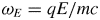 $\omega _E = qE / mc$ and
 $\omega _B=qB/m$. Integration is performed according to the particle proper time
 $\tau$. The initial 4-position is
 $(ct_0, x_0,y_0,z_0)$.
Note that our treatment proposed above works also for orthogonal fields but not for light-like fields for which both electromagnetic invariants vanish,  $I_1=\boldsymbol {E} \boldsymbol {\cdot } \boldsymbol {B} = 0$ and
 $I_2=E^2-c^2B^2=0$. For non-light-like fields, we can use the same algorithm, there always exists a frame where either the magnetic field or the electric field vanishes, obtained by a Lorentz boost. For instance, the vanishing magnetic field case
 $\boldsymbol {B}=\boldsymbol {0}$ is obtained by taking the limiting
 $\lim _{\omega _B \to 0}$ of the above expression thus leading to the 4-velocity
 \begin{gather} u^0 = \gamma_0 c [\cosh (\omega_E \tau) + \beta_0^z \sinh (\omega_E \tau)] \end{gather}
 \begin{gather}u^1 = \gamma_0 c \beta_0^x \end{gather}
 \begin{gather}u^2 = \gamma_0 c \beta_0^y \end{gather}
 \begin{gather}u^3 = \gamma_0 c [\sinh (\omega_E \tau) + \beta_0^z \cosh (\omega_E \tau)] \end{gather}
and to the 4-position
 \begin{gather} c(t-t_0) = \frac{\gamma_0 c}{\omega_E} [\sinh (\omega_E \tau) + \beta_0^z \cosh (\omega_E \tau) - \beta_0^z] \end{gather}
 \begin{gather}x-x_0 = \gamma_0 c \beta_0^x \tau \end{gather}
 \begin{gather}y-y_0 = \gamma_0 c \beta_0^y \tau \end{gather}
 \begin{gather}z-z_0 = \frac{\gamma_0 c}{\omega_E} [\cosh (\omega_E \tau) -1 + \beta_0^z \sinh (\omega_E \tau)] . \end{gather}
In the same way, the vanishing electric field  $\boldsymbol {E}=\boldsymbol {0}$ is treated with the limit
 $\lim _{\omega _E \to 0}$, leading to the 4-velocity
 \begin{gather} u^0 = \gamma_0 c \end{gather}
 \begin{gather}u^1 = \gamma_0 c [\beta_0^x \cos(\omega_B \tau) + \beta_0^y \sin (\omega_B \tau)] \end{gather}
 \begin{gather}u^2 = \gamma_0 c [-\beta_0^x \sin(\omega_B \tau) + \beta_0^y \cos (\omega_B \tau)] \end{gather}
 \begin{gather}u^3 = \gamma_0 c \beta_0^z \end{gather}
and to the 4-position
 \begin{gather} c(t-t_0) = \gamma_0 c \tau \end{gather}
 \begin{gather}x-x_0 = \frac{\gamma_0 c}{\omega_B} [\beta_0^x \sin(\omega_B \tau) - \beta_0^y \cos (\omega_B \tau) +\beta_0^y] \end{gather}
 \begin{gather}y-y_0 = \frac{\gamma_0 c}{\omega_B} [\beta_0^x \cos(\omega_B \tau) -\beta_0^x + \beta_0^y \sin (\omega_B \tau)] \end{gather}
 \begin{gather}z-z_0 = \gamma_0 c \beta_0^z \tau . \end{gather}
A full derivation of the equations in all field configurations is exposed in Gourgoulhon (Reference Gourgoulhon2010). In order to decide whether the field is null like or not, we compare both invariants with the field strength, applying a threshold  $\epsilon \ll 1$ such that, if
 $|\boldsymbol {E} \boldsymbol {\cdot } \boldsymbol {B}|<\epsilon \|\boldsymbol {E}\|\, \|\boldsymbol {B}\|$ and
 $|E^2-c^2B^2|<\epsilon \,(E^2+c^2B^2)$, the field is said to be light-like or null. As long as
 $\epsilon$ is chosen small enough at approximately
 $10^{-8}$ or
 $10^{-12}$, the results are insensitive to the precise value of the threshold prescription. Moreover, in most physical applications, the light-like field is rarely met over a large volume in space–time. It happens to be true sometimes at some points but becomes very quickly again non-light-like. Especially for our forthcoming applications to a PIC code, such a condition is highly unlikely. In some of our tests, we impose the external electromagnetic field, for instance for a plane wave. In such a case the field is and remains light-like without the plasma feedback, but this situation is highly idealized.
The above mentioned algorithm clearly makes the assumption that the electric and the magnetic fields are constant during a time step  ${\rm \Delta} \tau$ and evaluated at the particle 4-position
 $(t^n,x_i)$. The algorithm switches between two reference frames, the first one identified as the observer frame (
 $R$) and the second produces an electric field aligned with the magnetic field (
 $R'$). Note that a vanishing electric or magnetic field is only a special case included in the former.
At first, in the reference frame ( $R$) of the distant observer, the 4-position
 ${\boldsymbol X}$ and 4-velocity
 ${\boldsymbol U}$ of the particle is known as well as the electric field
 ${\boldsymbol E}$ and the magnetic field
 ${\boldsymbol B}$ at the particle's position. We then search for a reference frame (
 $R'$) in which
 ${\boldsymbol E'}$ and
 ${\boldsymbol B'}$ are parallel (or, if
 ${\boldsymbol E} \boldsymbol {\cdot } {\boldsymbol B}=0$, where
 ${\boldsymbol B'}$ or
 ${\boldsymbol E'}$ vanishes depending on the relative strength of both fields). The speed of frame (
 $R'$) with respect to frame (
 $R$) is noted
 ${\boldsymbol V}$. We align the
 $z$-axis of (
 $R$) with
 ${\boldsymbol V}$ via rotation through the Euler angles, performing a rotation with help on the matrix
 $ {\mathsf {\boldsymbol M}}_{\boldsymbol 1}$. A Lorentz boost
 ${\varLambda }({\boldsymbol V})$ switches to the reference frame (
 $R'$). In this latter frame the particle's 4-position is
 ${\boldsymbol X'}$ and its 4-velocity
 ${\boldsymbol U'}$. We then rotate the axes to align the new
 $z'$-axis with
 ${\boldsymbol E}$ and
 ${\boldsymbol B}$ with the rotation matrix
 ${\mathsf {\boldsymbol M}}_{\boldsymbol 2}$. We next update
 ${\boldsymbol X'}$ and
 ${\boldsymbol U'}$ to the new time step (
 $\tau + {\rm \Delta} \tau$) thanks to the (2.1) and (2.2) describing the trajectory of a particle where the electric and magnetic fields are parallel to the
 $z$-axis and assumed to be constant during
 ${\rm \Delta} \tau$, with
 $\tau$ the proper time of the particle,
 $u^i$ the
 $i$th component of the 4-velocity and
 $\boldsymbol \beta$ the normalized speed of the particle. Quantities with subscript 0 are initial conditions, and superscripts
 $x, y$ or
 $z$ denote a projection on the
 $x, y$ or
 $z$-axis respectively. Once
 ${\boldsymbol X'}$ and
 ${\boldsymbol U'}$ are computed, the frame axes are set back to their initial positions with inverse rotations given by the matrix
 ${\mathsf {\boldsymbol M}}_{\boldsymbol 2}^{-{\boldsymbol 1}}$, the inverse of the
 ${\mathsf {\boldsymbol M}}_{\boldsymbol 2}$ rotation matrix. We boost back to the reference frame (
 $R$) with the inverse Lorentz transformation
 ${\varLambda }(-{\boldsymbol V})$, since in (
 $R'$) the speed of (
 $R$) is
 $-{\boldsymbol V}$. And, again, we align the axes of (
 $R$) with their initial positions thanks to the rotation matrix
 ${\mathsf {\boldsymbol M}}_{\boldsymbol 1}^{-{\boldsymbol 1}}$ finding the particle's new 4-position
 ${\boldsymbol X}$ and 4-velocity
 ${\boldsymbol U}$.
The special case of the light-like field,  $\boldsymbol {E} \boldsymbol {\cdot } \boldsymbol {B} = 0$ and
 $E^2 = c^2 B^2$, must be treated separately because there exists no frame where
 $\boldsymbol {E}$ and
 $\boldsymbol {B}$ are parallel. In the code, to consider that the field is light-like we introduce
 $\epsilon \ll 1$ and we verify
 $\vert E^2 - c^2 B^2\vert < \epsilon \vert E^2 + c^2 B^2\vert$ and
 $\vert \boldsymbol {E} \boldsymbol {\cdot } \boldsymbol {B} \vert < \epsilon \vert \boldsymbol {E} \vert \vert \boldsymbol {B}\vert$ (verification that the cosine of the angle between
 $\boldsymbol {E}$ and
 $\boldsymbol {B}$ is close to 0). Exact solutions can be found in Pétri (Reference Pétri2020c) but they are recalled here for
 $\omega _B=\omega _E$. In Pétri (Reference Pétri2020c) we allow for a more general configuration with
 $\omega _B=\pm \omega _E$ taking into account possible left- or right-handed coordinate axes. With
 $\boldsymbol {B}$ along
 $\boldsymbol {e}_z$ and
 $\boldsymbol {E}$ along
 $\boldsymbol {e}_y$, the 4-velocity can directly be obtained by
 \begin{gather} u^0 = \gamma_0 c \left[1+(1-\beta_0^x)\frac{(\omega_B \tau)^2}{2}+\beta_0^y \omega_B \tau\right] \end{gather}
 \begin{gather}u^1 = \gamma_0 c \left[\beta_0^x+(1-\beta_0^x)\frac{(\omega_B \tau)^2}{2}+\beta_0^y \omega_B \tau\right] \end{gather}
 \begin{gather}u^2 = \gamma_0 c [\beta_0^y+(1-\beta_0^x)\omega_B \tau] \end{gather}
 \begin{gather}u^3 = \gamma_0 c \beta_0^z \end{gather}
as well as the 4-position
 \begin{gather} c(t-t_0) = \gamma_0 c \left[\tau + (1-\beta_0^x)\frac{\omega_B^2 \tau^3}{6} + \beta_0^y \frac{\omega_B \tau^2}{2}\right] \end{gather}
 \begin{gather}x-x_0 = \gamma_0 c \left[\beta_0^x \tau + (1-\beta_0^x)\frac{\omega_B^2 \tau^3}{6} + \beta_0^y \frac{\omega_B \tau^2}{2}\right] \end{gather}
 \begin{gather}y-y_0 = \gamma_0 c \left[\beta_0^y \tau + (1-\beta_0^x) \frac{\omega_B \tau^2}{2}\right] \end{gather}
 \begin{gather}z-z_0 = \gamma_0 c \beta_0^z \tau . \end{gather}
Here, the algorithm is simpler: the 4-position  $\boldsymbol {X}$, the 4-velocity
 $\boldsymbol {U}$ of the particle are known, as well as the
 $\boldsymbol {E}$ and
 $\boldsymbol {B}$ felt by the particle. We then perform a rotation of matrix
 ${\mathsf {\boldsymbol M}}$ to align
 $\boldsymbol {E}$ with
 $\boldsymbol {e}_z$ and
 $\boldsymbol {B}$ with
 $\boldsymbol {e}_y$. Next, we directly update the particles 4-position
 $\boldsymbol {X}$ and 4-velocity
 $\boldsymbol {U}$ to the next time step
 $(\tau +{\rm \Delta} \tau )$ and we then rotate back to the initial set of axes with
 ${\mathsf {\boldsymbol M}}^{-{\boldsymbol 1}}$.
It is important to note that this peculiar case is very uncommon in the simulations mentioned in 5. Indeed, when choosing  $\epsilon = 10^{-15}$, the algorithm never used this peculiar case. In fact, the light-like case is only found in very precise positions or far from the neutron star, at distances the particles did not reach by the end of the simulations and this part of the algorithm was added so as to be able to work in any field, especially plane waves.
Technically, for the computation of the new velocity and position, a convergence criterion is applied on the electromagnetic field to make sure that the assumption  ${\boldsymbol E}$ and
 ${\boldsymbol B}$ remaining almost constant is verified to a prescribed accuracy. To do so, we use a loop on the
 $\boldsymbol {E}$ and
 $\boldsymbol {B}$ fields: at first we move the particle at the 4-position
 $(ct, x, y, z )$ by taking
 $\boldsymbol {E}_0=\boldsymbol {E}(t,x,y,z)$ and
 $\boldsymbol {B}_0=\boldsymbol {B}(t,x,y,z)$, so the particle's 4-position becomes
 $(c(t+\textrm {d} t_0), x+\textrm {d} x_0, y+\textrm {d} y_0, z+\textrm {d} z_0)$. Then, we make the particle start again from
 $(ct, x, y, z )$ but we take the averaged fields:
 $\boldsymbol {E}_1=\boldsymbol {E}(t+\textrm {d} t_0/2,x+\textrm {d} x_0/2,y+\textrm {d} y_0/2,z+\textrm {d} z_0/2)$ and
 $\boldsymbol {B}_1=\boldsymbol {B}(t+\textrm {d} t_0/2,x+\textrm {d} x_0/2,y+\textrm {d} y_0/2,z+\textrm {d} z_0/2)$ for the incrementation of the time, updating the 4-position:
 $(c(t+\textrm {d} t_1), x+\textrm {d} x_1, y+\textrm {d} y_1, z+\textrm {d} z_1)$. Then again, the particle starts from
 $(ct, x, y, z )$ and we increment the time step with the fields being
 $\boldsymbol {E}_2=\boldsymbol {E}(t+\textrm {d} t_1/2,x+\textrm {d} x_1/2,y+\textrm {d} y_1/2,z+\textrm {d} z_1/2)$ and
 $\boldsymbol {B}_2=\boldsymbol {B}(t+\textrm {d} t_1/2,x+\textrm {d} x_1/2,y+\textrm {d} y_1/2,z+\textrm {d} z_1/2)$. Generally, for
 $k \neq 0$ incrementing the time step with the field
 $\boldsymbol {E}_k$ and
 $\boldsymbol {B}_k$ returns the 4-position
 $(c(t+\textrm {d} t_k), x+\textrm {d} x_k, y+\textrm {d} y_k, z+\textrm {d} z_k)$, and the fields are defined as
 $\boldsymbol {E}_{k+1}=\boldsymbol {E}(t+\textrm {d} t_k/2,x+\textrm {d} x_k/2,y+\textrm {d} y_k/2,z+\textrm {d} z_k/2)$ and
 $\boldsymbol {B}_{k+1}=\boldsymbol {B}(t+\textrm {d} t_k/2,x+\textrm {d} x_k/2,y+\textrm {d} y_k/2,z+\textrm {d} z_k/2)$. We keep the loop going while
 $\boldsymbol {B}_k \neq \boldsymbol {B}_{k-1}$ and
 $\boldsymbol {E}_k \neq \boldsymbol {E}_{k-1}$, which numerically translates to
 $\vert E_k^j-E_{k-1}^j \vert > \epsilon (\vert E_{k}^j \vert + \vert E_{k-1}^j \vert )$ and
 $\vert B_k^j-B_{k-1}^j \vert > \epsilon (\vert B_{k}^j \vert + \vert B_{k-1}^j \vert )$, with
 $\epsilon \ll 1$ (we chose
 $\epsilon =10^{-4}$), and
 $j=\{x,y,z\}$.
As a check of the implementation of our new algorithm, simulations were performed either in a constant and uniform field, or in a plane electromagnetic wave. Once the tests were passed, we applied our code to realistic astrophysical cases of rotating neutron stars using the Deutsch (Reference Deutsch1955) field solution, neglecting thus far the radiation reaction that will be included in a next step.
3 Test cases
We carried some simulations to test the code in cases where the trajectory of the particle is known analytically. Simple checks with only an electric or magnetic field or both were made, allowing for orthogonal or parallel geometries.
When the  ${\boldsymbol E}$ and
 ${\boldsymbol B}$ fields are parallel, in addition to the gyration around the magnetic field lines, the particle is accelerated along the electric field, so that particles describe a helix that becomes elongated with time, if not at first slowing down if its initial velocity is in the direction opposite to its acceleration.
If  ${\boldsymbol E}$ and
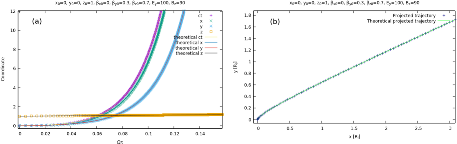
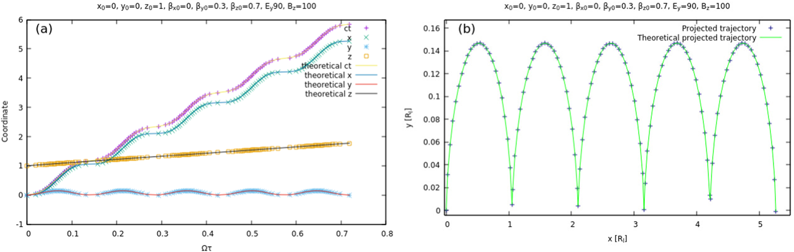
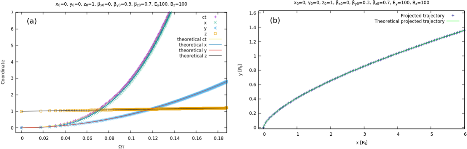
 ${\boldsymbol B}$ are orthogonal (as in figures 1, 2 and 3, where
 ${\boldsymbol E}$ is along the
 $y$-axis and
 ${\boldsymbol B}$ along the
 $z$-axis), three cases are possible:
(a)
${\boldsymbol E}$ dominant, as shown in figure 1, where the particle is accelerated along the ${\boldsymbol E}$ field but also drifts along ${\boldsymbol E} \times {\boldsymbol B}/E^2$;(b)
${\boldsymbol B}$ dominant, as in figure 2, where the particles moves in a cycloidal motion with the component of its speed along ${\boldsymbol E}$ switching between aligned and anti-aligned, and the other component being again a drift along ${\boldsymbol E} \times {\boldsymbol B}/B^2$;(a) in the special case of the light-like field (
$\boldsymbol {E} \boldsymbol {\cdot } \boldsymbol {B} = 0$ and $E^2 = c^2 B^2$), as in figure 3, where the trajectory of the particle is not periodic, in a similar fashion as the case where ${\boldsymbol E}$ is dominant with an increasing speed along ${\boldsymbol B}$ and again a drift along ${\boldsymbol E} \times {\boldsymbol B}$.


Evolution of a particle in a dominant electric field,  $x_0=0$,
 $y_0=0$,
 $z_0=1$,
 $\beta ^x_{0}=0$,
 $\beta ^y_{0}=0.3$,
 $\beta ^z_{0}=0.7$,
 ${qE_y}/{cm}=100$,
 ${qB_z}/{m}=90$. Theoretical and simulated 4-position as function of the proper time
 $\tau$ (a). Projection of the trajectory of the particle in the
 $x$–
 $y$ plane (b).

Evolution of a particle in a dominant magnetic field,  $x_0=0$,
 $y_0=0$,
 $z_0=1$,
 $\beta ^x_{0}=0$,
 $\beta ^y_{0}=0.3$,
 $\beta ^z_{0}=0.7$,
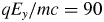 ${qE_y}/{mc}=90$,
 ${qB_z}/{m}=100$. Theoretical and simulated 4-position as function of the proper time
 $\tau$ (a). Projection of the trajectory of the particle in the
 $x$–
 $y$ plane (b).

Evolution of a particle in a light-like field,  $x_0=0$,
 $y_0=0$,
 $z_0=1$,
 $\beta ^x_{0}=0$,
 $\beta ^y_{0}=0.3$,
 $\beta ^z_{0}=0.7$,
 ${qE_y}/{cm}=100$,
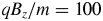 ${qB_z}/{m}=100$. Theoretical and simulated 4-position as function of the proper time
 $\tau$ (a). Projection of the trajectory of the particle in the
 $x$–
 $y$ plane (b).

In addition to the tests in constant uniform fields, simulations were undertaken with linearly and circularly polarized plane electromagnetic waves, for which exact solutions are known (Uzan & Deruelle Reference Uzan and Deruelle2014).
Consider a linearly polarized plane wave propagating along the  $\boldsymbol {e}_{x}$ direction such that the 4-vector potential is
 $A^\alpha =(0,0,({E}/{\omega })\cos \xi ,0)$. The phase is
 $\xi =\omega t-kx$. The electromagnetic field is given by
 \begin{gather} \boldsymbol{E} = E \sin \xi \boldsymbol{e}_{y} \end{gather}
 \begin{gather}\boldsymbol{B} = \frac{E}{c} \sin \xi \boldsymbol{e}_{z} . \end{gather}
Initially, the particle is at rest with a 4-velocity  $u^\alpha _0=(c,\mathbf 0)$. Introducing the strength parameter of the wave by the ratio
 \begin{equation} a = \frac{q E}{mc\omega}, \end{equation}
the 4-velocity has components
 \begin{gather} u^x = \frac{a^2}{2} c (\cos \xi - 1 )^2 \end{gather}
 \begin{gather}u^y = -a c (\cos \xi - 1 ) \end{gather}
 \begin{gather}u^0 = c + u^x . \end{gather}
The Lorentz factor is deduced from  $\gamma c = u^0$.
Consider now a circularly polarized plane wave propagating in the  $\boldsymbol {e}_{x}$ direction such that the vector potential has components
 $A^\alpha =(0,0,({E}/{\omega })\cos \xi , ({E}/{\omega }) \sin \xi )$ and the phase
 $\xi =\omega t-kx$. The electromagnetic field is then given by
 \begin{gather} \boldsymbol{E} = E ( \sin \xi \boldsymbol{e}_{y} - \cos \xi \boldsymbol{e}_{z} ) \end{gather}
 \begin{gather}\boldsymbol{B} = \frac{E}{c} ( \sin \xi \boldsymbol{e}_{z} + \cos \xi \boldsymbol{e}_{y} ) . \end{gather}
Initially, the particle is at rest with 4-velocity  $u^\alpha _0=(c,\mathbf 0)$. The time evolution of the components of this 4-velocity will be
 \begin{gather} u^x = a^2 c (1 - \cos \xi ) = a u^y \end{gather}
 \begin{gather}u^y = a c (1 - \cos \xi ) \end{gather}
 \begin{gather}u^z = - a c \sin \xi \end{gather}
 \begin{gather}u^0 = c + u^x . \end{gather}
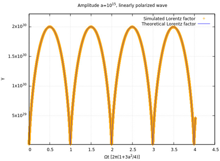
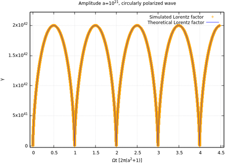
Simulations of linearly and circularly polarized plane waves were carried out, as shown in figures 4 and 5. In these waves, the particle undergoes a series of accelerations and brakings.
Lorentz factor of a particle in a linearly polarized plane electromagnetic wave of strength parameter  $a=10^{15}$.

Lorentz factor of a particle in a circularly polarized plane electromagnetic wave of strength parameter  $a=10^{21}$.

The particle's Lorentz factor reaches a maximum value of
 \begin{equation} \gamma=1+2a^2. \end{equation}
This shows that the code works well in ultra-strong fields with little to no error.
In addition, the cases of elliptically polarized waves can be treated in the code. The equation of the fields of such waves is given by
 \begin{gather} \boldsymbol{E} = E ( \sin \xi \boldsymbol{e}_{y} - \alpha \cos \xi \boldsymbol{e}_{z} ) \end{gather}
 \begin{gather}\boldsymbol{B} = \frac{E}{c} (\sin \xi \boldsymbol{e}_{z} + \alpha \cos \xi \boldsymbol{e}_{y} ) , \end{gather}
with  $0 \leq \alpha \leq 1$. The case
 $\alpha =1$ gives the circular wave whereas the case
 $\alpha =0$ returns the linearly polarized wave. For any kind of polarization, the maximum Lorentz factor of the particle is still
 $\gamma =1+2a^2$, however, the evolution of the particle's Lorentz factor is the following:
 \begin{equation} \gamma=1+a^2 (1-\cos\xi)-\frac{a^2}{2} (1-\alpha^2)\sin^2\xi , \end{equation}
which is (157) of Michel & Li (Reference Michel and Li1999) except for a typo in the sign of the last term. More details about plane waves and how to find these equations can be found in Michel & Li (Reference Michel and Li1999).
In the case of plane electromagnetic waves other algorithms have trouble at strength parameters above  $a=25$ (Arefiev et al. Reference Arefiev, Cochran, Schumacher, Robinson and Chen2015) whereas our scheme easily exceeds this value of
 $a$ with short computational times.
4 Convergence and error of the algorithm
We study the convergence of our algorithm in simple test cases where analytical solutions are known. For instance, let us track a particle of charge  $q$ and mass
 $m$ subject to an acceleration in an electric field
 $\boldsymbol {E}$ assumed to grow linearly in proper time
 $\tau$ such that
 \begin{equation} \boldsymbol{E}(\tau) = E(\tau) \boldsymbol{e}_z, \end{equation}
with
 \begin{equation} \frac{q}{mc}E(\tau) = \alpha \tau . \end{equation}
We choose this form of field since a constant field will give no error, for the code is based on analytical solutions in constant fields. At  $\tau =0$, the particle is at
 $x^{\mu }=(0 \enspace 0 \enspace 0 \enspace 0)$ and its 4-velocity is
 $u^{\mu }=(c \enspace 0 \enspace 0 \enspace 0)$. In this configuration, the Faraday tensor is
 \begin{equation} {F}^{\mu \nu}= \begin{pmatrix} 0 & 0 & 0 & -E(\tau)/c \\ 0 & 0 & 0 & 0 \\ 0 & 0 & 0 & 0 \\ E(\tau)/c & 0 & 0 & 0 \end{pmatrix}. \end{equation}
Starting from the equation of motion
 \begin{equation} \frac{\textrm{d} u^{\mu}}{\textrm{d} \tau}=\frac{q}{m} {F}^{\mu \nu}u_{\nu}, \end{equation}
when looking only at  $u^t$ and
 $u^z$ we find
 \begin{gather} \frac{\textrm{d} u^t}{\textrm{d} \tau} = - \frac{q E(\tau)}{mc} u_z = -\alpha \tau u_z = \alpha \tau u^z \end{gather}
 \begin{gather}\frac{\textrm{d} u^z}{\textrm{d} \tau} = \frac{q E(\tau)}{mc} u_t =\alpha \tau u_t = \alpha \tau u^t. \end{gather}
We then define
 \begin{gather} {\rm \Delta} = u^t-u^z \end{gather}
 \begin{gather}\varSigma = u^t+u^z. \end{gather}
So we can obtain with (4.5a) $-$(4.5b) and (4.5a)
 $+$(4.5b)
 \begin{gather} \frac{\textrm{d} {\rm \Delta}}{\textrm{d} \tau} = -\alpha \tau {\rm \Delta} \end{gather}
 \begin{gather}\frac{\textrm{d} \varSigma}{\textrm{d} \tau} = \alpha \tau \varSigma, \end{gather}
which is solved to give
 \begin{gather} {\rm \Delta} (\tau) = \delta \,\textrm{e}^{-\alpha \tau^2/2} \end{gather}
 \begin{gather}\varSigma (\tau) = \sigma \,\textrm{e}^{\alpha \tau^2/2}. \end{gather}
At  $\tau =0$, we find
 \begin{equation} \delta = \sigma = \gamma_0. \end{equation}
Noticing that
 \begin{gather} u^t = \frac{\varSigma + {\rm \Delta} }{2} = \gamma_0 \frac{\textrm{e}^{\alpha \tau^2/2} + \textrm{e}^{-\alpha \tau^2/2} }{2} \end{gather}
 \begin{gather}u^z = \frac{\varSigma - {\rm \Delta} }{2} = \gamma_0 \frac{\textrm{e}^{\alpha \tau^2/2} - \textrm{e}^{-\alpha \tau^2/2} }{2}, \end{gather}
the expression for the Lorentz factor and the four velocity along  $z$ are
 \begin{gather} u^t = \gamma_0 c \cosh(\alpha \tau^2/2) \end{gather}
 \begin{gather}u^z = \gamma_0 c \sinh(\alpha \tau^2/2). \end{gather}
After another integration, we get the position of the particle
 \begin{gather} ct = \gamma_0 c \sqrt{\frac{\rm \pi}{8 \alpha}} [ \text{erf}(\tau \sqrt{\alpha / 2}) + \text{erfi}(\tau \sqrt{\alpha / 2}) ] \end{gather}
 \begin{gather}z = \gamma_0 c \sqrt{\frac{\rm \pi}{8 \alpha}} [ \text{erfi}(\tau \sqrt{\alpha / 2}) - \text{erf}(\tau \sqrt{\alpha / 2}) ] , \end{gather}
where  $\text {erf}$ and
 $\text {erfi}$ are defined (with
 $\textrm {i}$ the imaginary unit) by
 \begin{gather} \text{erf}(\tau)=\frac{2}{\sqrt{\rm \pi}}\int_{0}^{\tau} \exp(-t^2)\,\textrm{d} t \end{gather}
 \begin{gather}\text{erfi}(\tau)=\frac{\text{erf}(\textrm{i}\tau)}{\textrm{i}} . \end{gather}
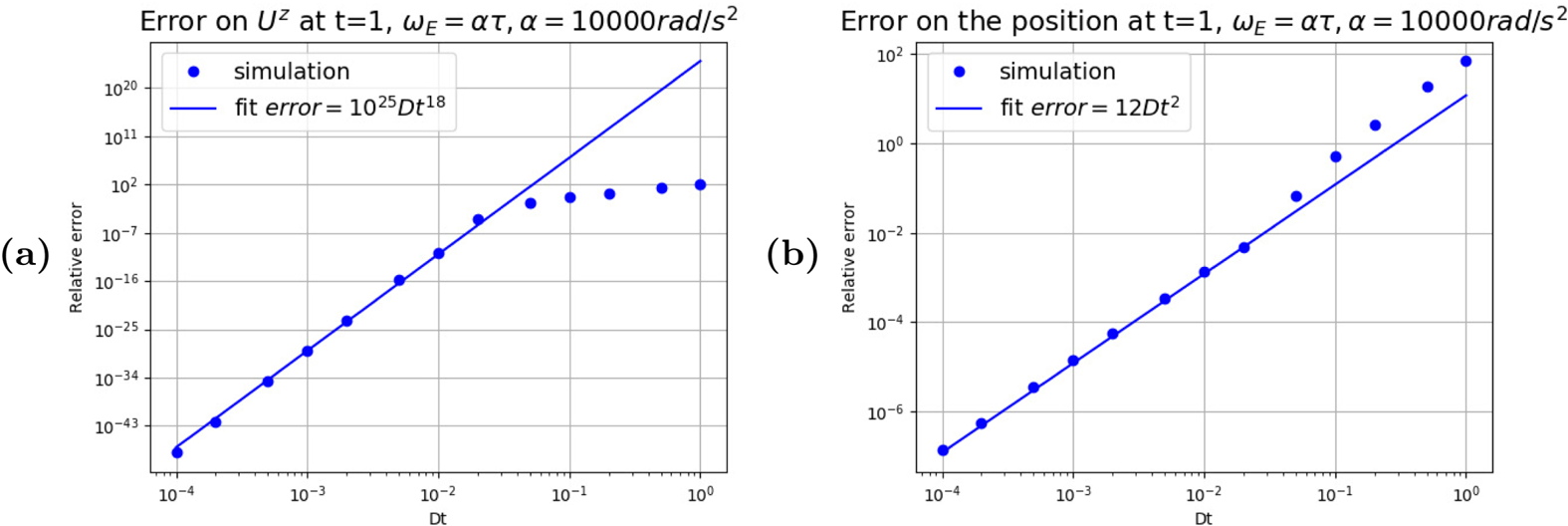
When comparing (4.11b) and (4.12b) to the outcome of the simulations, we can get the error  $\delta \alpha$ thanks to the following formula:
 \begin{equation} \delta \alpha=\frac{\vert \alpha_{\textrm{measured}} - \alpha_{\textrm{theoretical}} \vert}{ \vert \alpha_{\textrm{theoretical}} \vert}. \end{equation}
When  $\alpha$ is taken to be
 $u^z$ or
 $z$ we obtain the plots of figure 6, highlighting a fast decrease on the error on the 4-velocity; however, the error on the 4-position shows that the scheme of the simulation is of order 2.
Relative error on the speed and on the position of the particle in an electric field aligned with  $\boldsymbol {e}_z$ where
 $\omega _E = \alpha \tau$,
 $\alpha =10^4$.

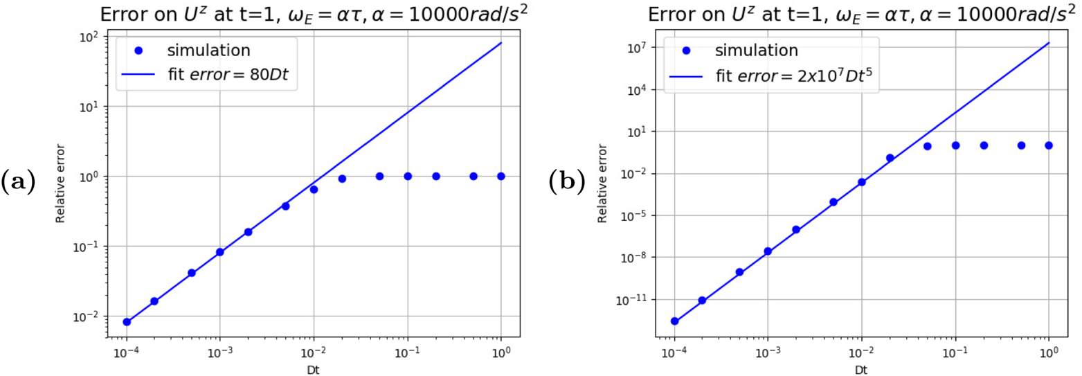
A more in-depth analysis showed that the number of iterations through the field convergence loop discussed in 2 has an influence on the order of the algorithm, explaining why such a high order is found in figure 6. Simulations where no convergence is applied or where at most three iterations through the convergence loop are made are, respectively, of order 1 or 5, as shown by figure 7.
Relative error on the speed of the particle in an electric field aligned with  $\boldsymbol {e}_z$ where
 $\omega _E = \alpha \tau$,
 $\alpha =10^4$. (a) No convergence loop on the field. (b) At most three iterations in the convergence loop.

Other studies of the rate of convergence to the analytical solutions can be found in Pétri (Reference Pétri2020c) for a linearly and a circularly polarized wave. There, it is shown that the error is second order in time.
5 Rotating neutron star fields
5.1 Vacuum rotating electromagnetic field solution
Eventually, we implemented the Deutsch field in our code in order to mimic a rotating magnet in vacuum. The exact solution for the rotating dipole in vacuum is given by Deutsch (Reference Deutsch1955). The corresponding electromagnetic field, written in a complex form, reads
 \begin{equation} B_r(\boldsymbol{r},t) = 2 B \left[ \frac{R^3}{r^3} \cos\chi \cos\vartheta + \frac{R}{r} \frac{h^{(1)}_1(kr)}{h^{(1)}_1(kR)} \sin\chi \sin \vartheta \, \textrm{e}^{\textrm{i}\psi} \right] \end{equation}
 \begin{align} B_\vartheta(\boldsymbol{r},t) &= B \left[ \frac{R^3}{r^3} \cos\chi \sin\vartheta \vphantom{\left( \frac{R}{r} \frac{\dfrac{\textrm{d}}{\textrm{d} r} \left( r h^{(1)}_1(kr) \right)}{h^{(1)}_1(kR)} + \frac{R^2}{r_{L}^2} \frac{h^{(1)}_2(kr)}{\left.\dfrac{\textrm{d}}{\textrm{d} r} \left( r h^{(1)}_2(kr) \right) \right|_{R}} \right)}\right. \nonumber\\ &\quad +\left. \left( \frac{R}{r} \frac{\dfrac{\textrm{d}}{\textrm{d} r} \left( r h^{(1)}_1(kr) \right)}{h^{(1)}_1(kR)} + \frac{R^2}{r_{L}^2} \frac{h^{(1)}_2(kr)}{\left.\dfrac{\textrm{d}}{\textrm{d} r} \left( r h^{(1)}_2(kr) \right) \right|_{R}} \right) \sin\chi \cos \vartheta \, \textrm{e}^{\textrm{i}\psi} \right] \end{align}
 \begin{equation} B_\varphi(\boldsymbol{r},t) = B \left[ \frac{R}{r} \frac{\dfrac{\textrm{d}}{\textrm{d} r} ( r h^{(1)}_1(kr) )}{h^{(1)}_1(kR)} + \frac{R^2}{r_{L}^2} \frac{h^{(1)}_2(kr)}{\left.\dfrac{\textrm{d}}{\textrm{d} r} \left( r h^{(1)}_2(kr) \right) \right|_{R}}\cos 2\vartheta \right] \textrm{i}\sin\chi \, \textrm{e}^{\textrm{i}\psi} \end{equation}
 \begin{align} E_r(\boldsymbol{r},t) &= \varOmega B R \left[ \left( \frac{2}{3} - \frac{R^2}{r^2} ( 3 \cos^2\vartheta - 1 ) \right) \frac{R^2}{r^2} \cos\chi \vphantom{\frac{ h^{(1)}_2(k\,r)}{\left.\dfrac{\textrm{d}}{\textrm{d} r} \left( r h^{(1)}_2(kr) \right) \right|_{R}}}\right. \nonumber\\ &\quad + \left. 3 \sin\chi \sin 2\vartheta \, \textrm{e}^{\textrm{i}\psi} \frac{R}{r} \frac{ h^{(1)}_2(k\,r)}{\left.\dfrac{\textrm{d}}{\textrm{d} r} \left( r h^{(1)}_2(kr) \right) \right|_{R}} \right] \end{align}
 \begin{align} E_\vartheta(\boldsymbol{r},t) &= \varOmega B R \left[ - \frac{R^4}{r^4} \sin 2\vartheta \cos\chi \vphantom{\left(\frac{R}{r} \frac{\dfrac{\textrm{d}}{\textrm{d} r} \left( r h^{(1)}_2(kr) \right)} {\left.\dfrac{\textrm{d}}{\textrm{d} r} \left( r h^{(1)}_2(kr) \right)\right|_{R}} \cos 2\vartheta - \frac{h^{(1)}_1(kr)}{h^{(1)}_1(kR)} \right)}\right. \nonumber\\ &\quad \left.+ \sin\chi\, \textrm{e}^{\textrm{i}\psi} \left(\frac{R}{r} \frac{\dfrac{\textrm{d}}{\textrm{d} r} \left( r h^{(1)}_2(kr) \right)} {\left.\dfrac{\textrm{d}}{\textrm{d} r} \left( r h^{(1)}_2(kr) \right)\right|_{R}} \cos 2\vartheta - \frac{h^{(1)}_1(kr)}{h^{(1)}_1(kR)} \right) \right] \end{align}
 \begin{equation} E_\varphi(\boldsymbol{r},t) = \varOmega B R \left[\frac{R}{r}\frac{\dfrac{\textrm{d}}{\textrm{d} r} \left(r h^{(1)}_2(kr) \right)}{\left.\dfrac{\textrm{d}}{\textrm{d} r} \left( r h^{(1)}_2(kr) \right)\right|_{R}} - \frac{h^{(1)}_1(kr)}{h^{(1)}_1(kR)} \right] \textrm{i} \sin\chi \cos\vartheta \, \textrm{e}^{\textrm{i}\psi}, \end{equation}
where  $h^{(1)}_\ell$ are the spherical Hankel functions for outgoing waves (Arfken & Weber Reference Arfken and Weber2005),
 $kr_{L}=1$ and the phase is
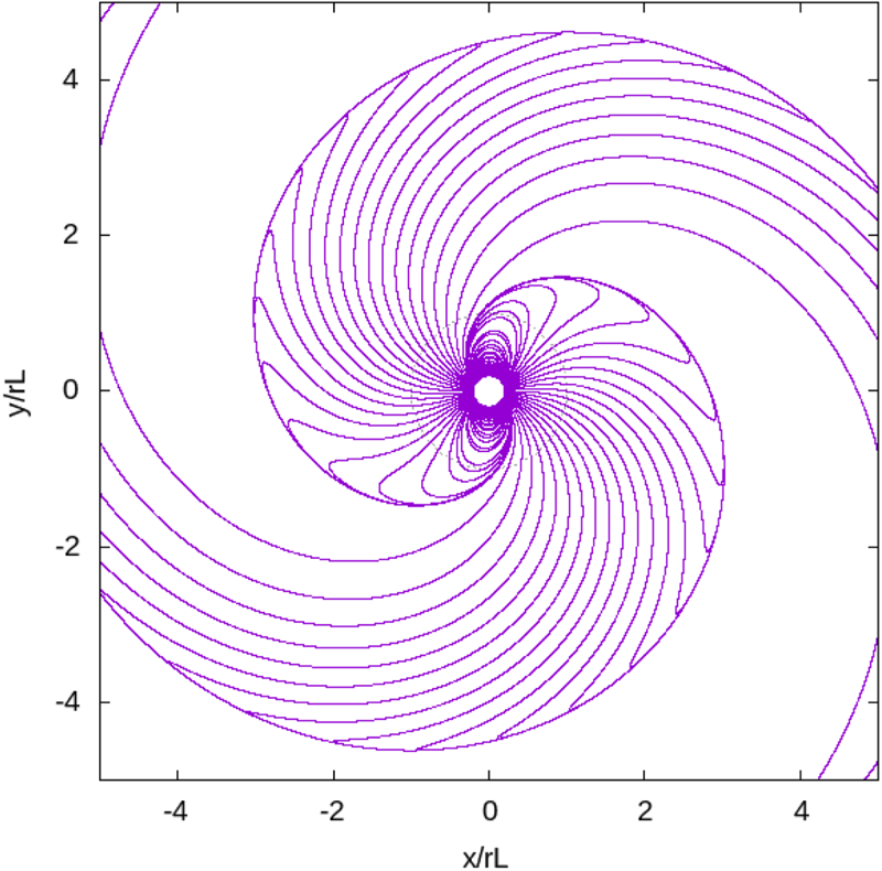
 $\psi =-\varOmega t$. An example of magnetic field lines for a perpendicular rotator is shown in figure 8.
Magnetic field line of an orthogonal rotator with  $r_{L}=5R$.

Our aim for these simulations was to investigate the behaviour of particles close to the neutron star, especially to find the final Lorentz factor the particles were able to reach as well as the influence of their initial position on their final position and energy.
As expected, the particles could either be ejected far from the neutron star, reaching an almost ballistic trajectory, or crash onto the neutron star surface or be trapped around the pulsar.
In all of our simulations, we work with a millisecond pulsar for which  $r_{L}=10 \ R=100\ \text {km}$ so
 $\varOmega =3000\ \text {rad}\ \text {s}^{-1}$ and the period is approximately
 $P\approx 2.1\ \text {ms}$. We choose the magnetic field strength at the equator to be
 $B=10^{5}\ \text {T}$.
5.2 Settings
The main purpose of our simulations was to investigate the evolution of five types of particles: electrons, protons, antiprotons, fully ionized iron  ${}^{56}$Fe and fictive particles with the charge of a proton, but
 $10^6$ times its mass (mentioned in 5.3.1). The inclination angle of the neutron stars is taken in the set
 $\chi =\{0^{\circ }, 30^{\circ }, 60^{\circ }, 90^{\circ }, 120^{\circ }, 150^{\circ }, 180^{\circ }\}$.
We tried three different initial set-ups by imposing the starting positions of the particles
(i) The first set-up used 2.048 particles for each obliquity and type of charges, following the same regular pattern. These particles were distributed uniformly in spherical coordinates, radius (
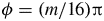
$r=(2+k)R$, $k \in [\![ 0;7 ]\!]$), colatitude ($\theta =({l}/{9}){\rm \pi}$ , $l \in [\![ 1;8 ]\!]$) and azimuth ($\phi = ({m}/{16}) {\rm \pi}$, $m \in [\![ 0;31 ]\!]$). (Note that this does not correspond to a uniform distribution in space.)(ii) The second set-up also used 2.048 particles per obliquity. However, they were randomly placed in space. The radius follows a uniform distribution
$r\in [2R;10R]$, the azimuth $\phi$ also follows a uniform distribution $\phi \in [0;2 {\rm \pi} ]$, however, for the colatitude, we use another variable $u$, following a uniform probability $u\in [0;1]$ and then we set the initial colatitude of the particle to be $\theta = \arccos (1-2u)$ so as to avoid artificial particle over-densities close to the rotation axis because of the singularity along this axis.(iii) The third set-up only used protons, but with 16.384 particles for each inclination, with the same random distribution as in point (ii).







Unless they crashed onto the neutron star, these test particles were free to evolve for a time  $T=15\ \Omega ^{-1}$ in normalized units, which is
 $T=5\ \text {ms} \simeq 2.39$ periods.
5.3 Regularly placed particles
5.3.1 Particle distribution functions and symmetries
The particle distribution functions  $f(\gamma ) = \textrm {d} N(\gamma )/\textrm {d}\gamma$, where
 $\textrm {d} N(\gamma )$ is the number of particles with a Lorentz factor in the range
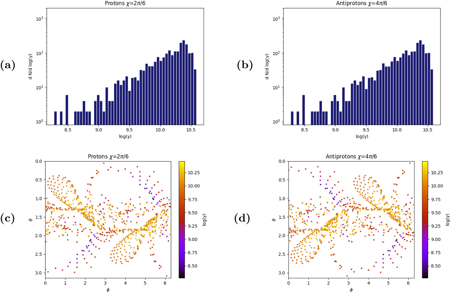
 $[\gamma ,\gamma +\textrm {d}\gamma ]$, and final positions are shown in figure 9. For particles of the same mass
 $m$ but opposite charge
 ${\pm }q$, the behaviour is symmetric, meaning that if, for an inclination
 $\chi$, a proton starts at position
 $(r_i,\theta _i,\phi _i)$ and ends at position
 $(r_f,\theta _f,\phi _f)$, for an inclination such that
 $\chi '={\rm \pi} -\chi$ an antiproton with an initial position
 $(r_i' = r_i,\theta _i' = {\rm \pi} -\theta _i,\phi _i'=\phi _i)$ will end at
 $(r_f'=r_f,\theta _f'={\rm \pi} -\theta _f,\phi _f'=\phi _f)$. Thus we only need to investigate a particle, its antiparticle returning redundant results, which is expected according to the symmetry arguments discussed in Laue & Thielheim (Reference Laue and Thielheim1986). Another symmetry relative to the centre of the neutron star is also noticeable in figures 9, 12 and 14 and tells us that, for an inclination
 $\chi$, if a particle is injected in
 $(r_i,\theta _i,\phi _i)$ and ends at
 $(r_f,\theta _f,\phi _f)$, a particle injected in
 $(r_i,{\rm \pi} -\theta _i,{\rm \pi} +\phi _i)$ will end at
 $(r_f,{\rm \pi} -\theta _f,{\rm \pi} +\phi _f)$. Again, this was discussed in Laue & Thielheim (Reference Laue and Thielheim1986).
Comparison between protons around a pulsar of inclination  $\chi =60^{\circ }$, and antiprotons around a pulsar of inclination
 $\chi =120^{\circ }$ to highlight their symmetrical behaviour. (a) Proton Lorentz factor distribution function. (b) Antiproton Lorentz factor distribution function. (c) Proton ejection map. (d) Antiproton ejection map. The ejection maps are the final latitudes
 $\theta$ and azimuths
 $\phi$ of particles that went beyond the light cylinder. These particles have an almost radial trajectory.

5.3.2 Final Lorentz factors
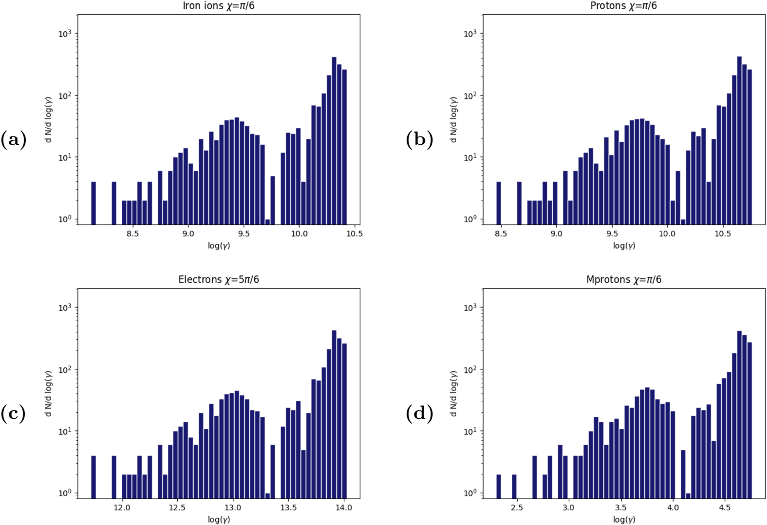
In the simulations, we explored the dependence of the final Lorentz factor with respect to the particle charge to mass ratio  $q/m$. Results of our computations showed that the iron
 ${}^{56}$Fe reaches Lorentz factors of
 $\gamma _\textrm {Fe} \sim 10^{10.5}$, protons and antiprotons up to
 $\gamma _{p} \sim 10^{10.7}$ and electrons up to
 $\gamma _{e} \sim 10^{14}$. As a check for the scaling we also tried fictive particles of artificially very high mass
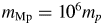 $m_\textrm {Mp}=10^6 m_p$ and charge
 $q_\textrm {Mp} = q_{p} = +e$ reaching only Lorentz factors up to
 $\gamma _\textrm {Mp} \sim 10^{4.7}$.
As anticipated, particles with high charge to mass ratio are accelerated more efficiently. In fact, the different spectra have similar shapes simply shifted along the  $\log (\gamma )$ axis. This is visible by comparing for instance figures 10(a) and 10(b) showing the distribution functions for iron and protons respectively. For these spectra, the difference is
 ${\rm \Delta} \log (\gamma ) \sim 0.33 \sim \log (2.15)$ meaning that
 $\gamma _{p}\sim 2.15 \gamma _{\textrm {Fe}}$. When comparing figures 10(b) to 10(d) for protons and massive particles, the shift is
 ${\rm \Delta} \log (\gamma ) \sim 6$ so
 $\gamma _{p} \sim 10^{6} \gamma _{\textrm {Mp}}$.
Comparison of different particle distribution functions following the regular placement: (a)  ${}^{56}$Fe ions with
 $\chi =30^{\circ }$, (b) Protons with
 $\chi =30^{\circ }$, (c) Electrons with
 $\chi =150^{\circ }$, (d) Fictive particle (
 $q_{\textrm {Mp}}=q_p$,
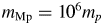 $m_{\textrm {Mp}}=10^{6}m_p$) with
 $\chi =30^{\circ }$.

As for protons and iron nuclei, and taking into account the symmetrical behaviour of particles of opposite charge, Lorentz factor distribution functions of protons and electrons show similar features for inclination such as  $\chi _e = {\rm \pi} - \chi _p$ (
 $\chi _e$ is the inclination of the pulsar for the electron and
 $\chi _p$ for the proton) but shifted by an amount
 ${\rm \Delta} \log (\gamma ) \sim 3.3 \sim \log (1836)$; compare figure 10(c) with 10(b).
As an example, in figure 10(b) for protons, when  $\chi ={\rm \pi }/{6}$, two lobes are visible in the spectrum: one from
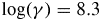 $\log (\gamma )=8.3$ to
 $\log (\gamma )=10.1$ and the other from
 $\log (\gamma )=10.2$ to
 $\log (\gamma )=10.7$. For electrons in figure 10(c), with
 $\chi ={5{\rm \pi} }/{6}$ the lobes also appear but from
 $\log (\gamma )=11.6$ to
 $\log (\gamma )=13.5$ and from
 $\log (\gamma )=13.5$ to
 $\log (\gamma )=14$. This difference shows that
 $\gamma _e \sim 1836 \gamma _p$ (
 $\gamma _e$ is the Lorentz factor of electrons) for
 $\chi _e= {\rm \pi} - \chi _p$.
Noticing the following ordering
 \begin{equation} \frac{q_{p}/m_{p}}{q_{\textrm{Fe}}/m_{\textrm{Fe}}}=\frac{56}{26} \sim 2.154,\quad \frac{|q_{e}/m_{e}|}{|q_{p}/m_{p}|} \sim 1836,\quad \frac{q_{p}/m_{p}}{q_{\textrm{Mp}}/m_{\textrm{Mp}}} = 10^6, \end{equation}
we conclude that the final Lorentz factor of the test particles is proportional to the strength parameter of these particles, as long as they are relativistic.
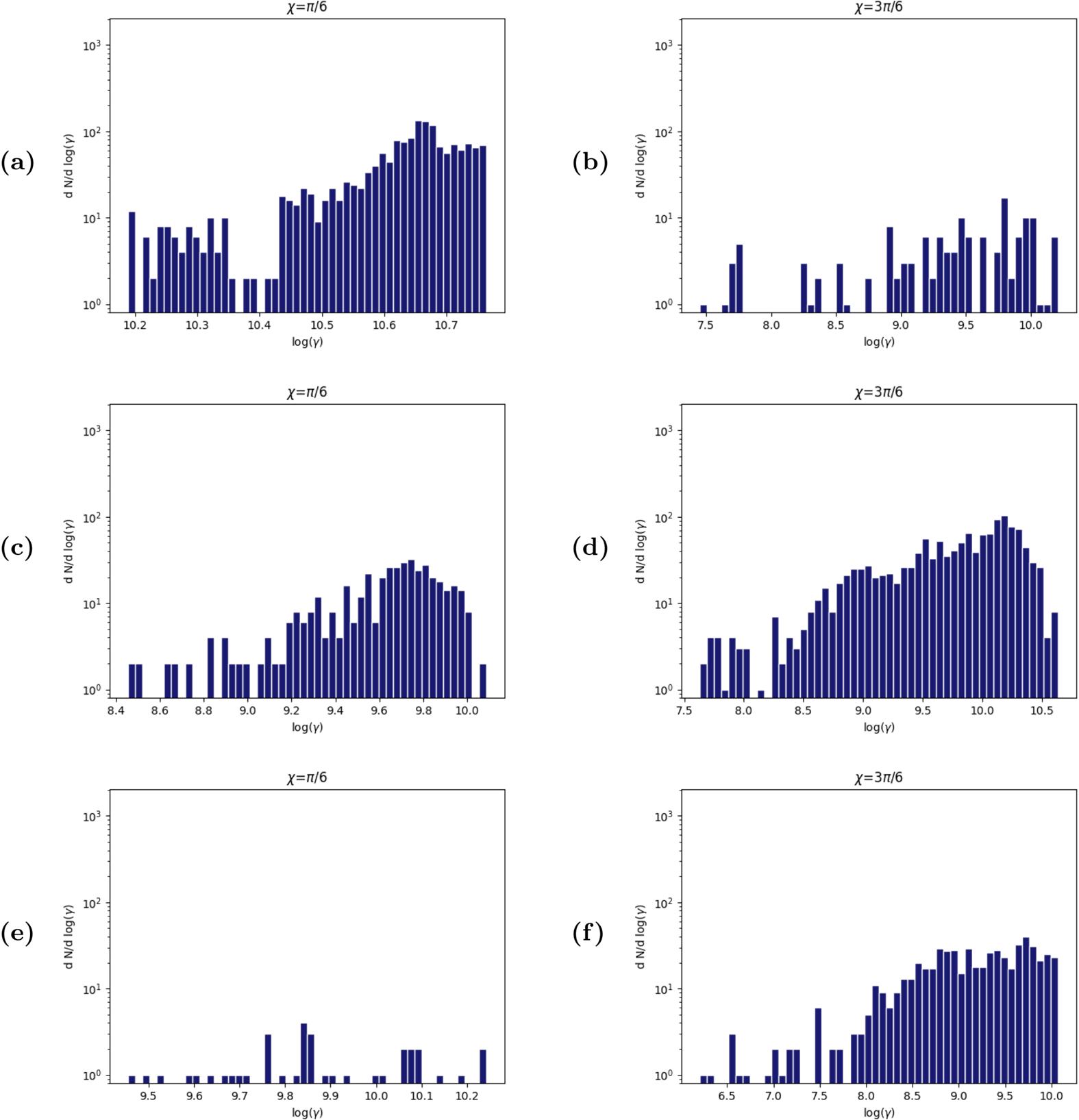
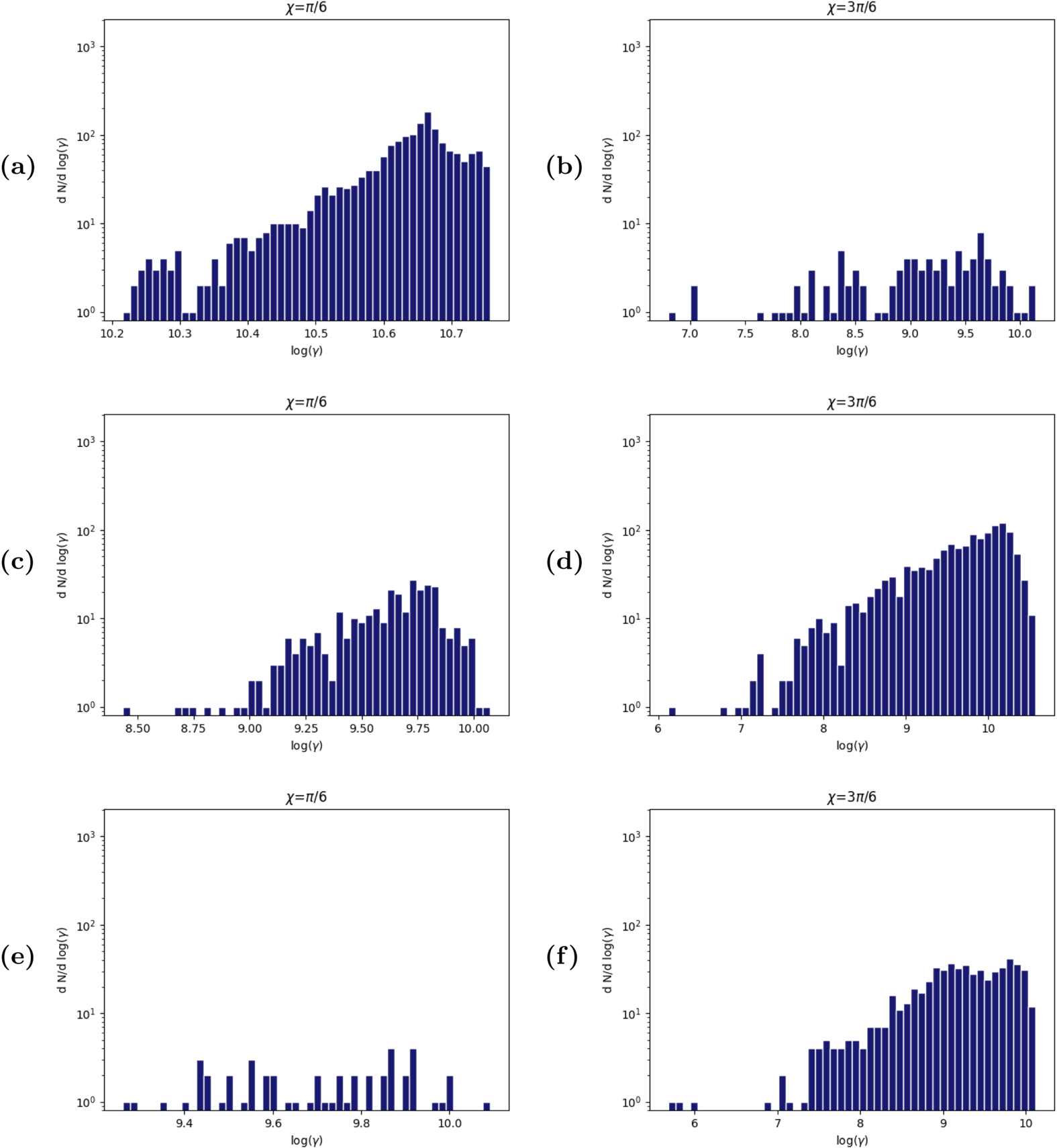
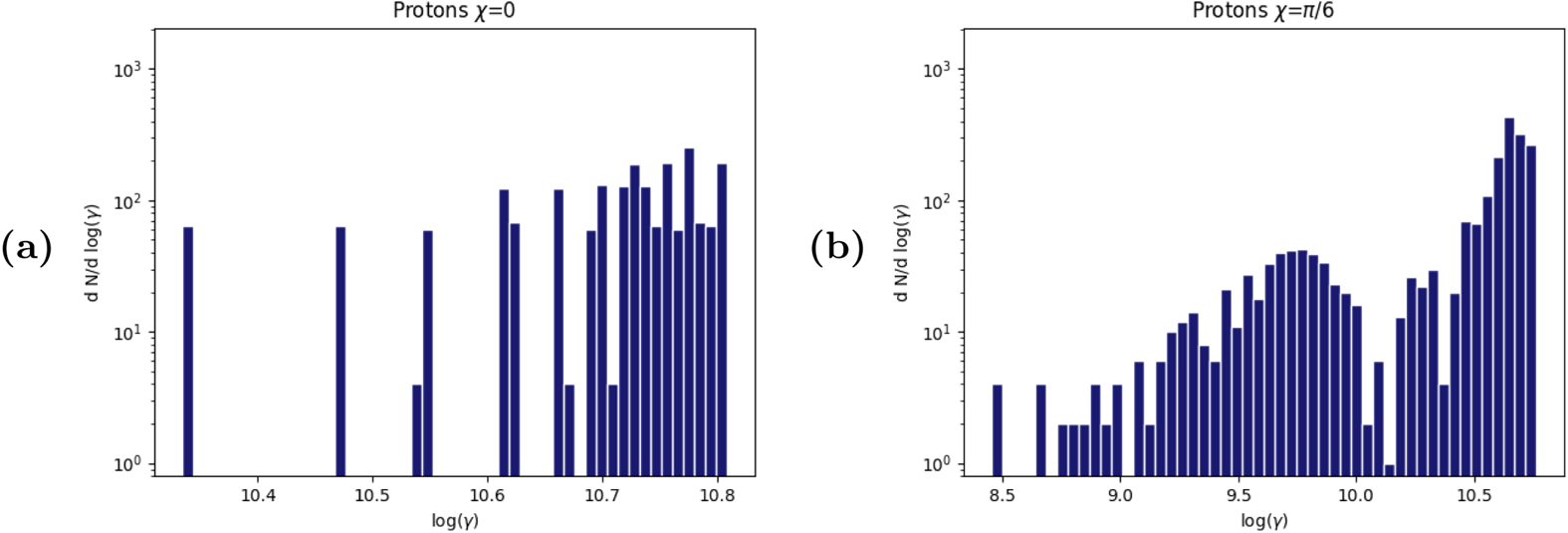
In complement, the spectra were analysed depending on whether the particles were ejected, trapped or crashed, as in figure 11. For protons, at inclinations  $\chi =\{0, {\rm \pi }/{6}, {\rm \pi }/{3} \}$ the most energetic particles were those falling on the neutron star (at
 $\chi =0^{\circ }$ all particles crashed with
 $10.3 \leq \log (\gamma ) \leq 10.8$). For
 $\chi =30^{\circ }$ falling particles are responsible for the high Lorentz factor lobe of the spectra. At
 $\chi =90^{\circ }$, however, crashing particles had similar energies as the ejected or trapped ones.
Proton distribution functions depending on their final state. (a) Crashed,  $\chi =30^{\circ }$, (b) crashed,
 $\chi =90^{\circ }$, (c) ejected,
 $\chi =30^{\circ }$, (d) ejected,
 $\chi =90^{\circ }$, (e) trapped,
 $\chi =30^{\circ }$, (f) trapped,
 $\chi =90^{\circ }$, for a regular pattern of particles.

5.3.3 Positions of particles
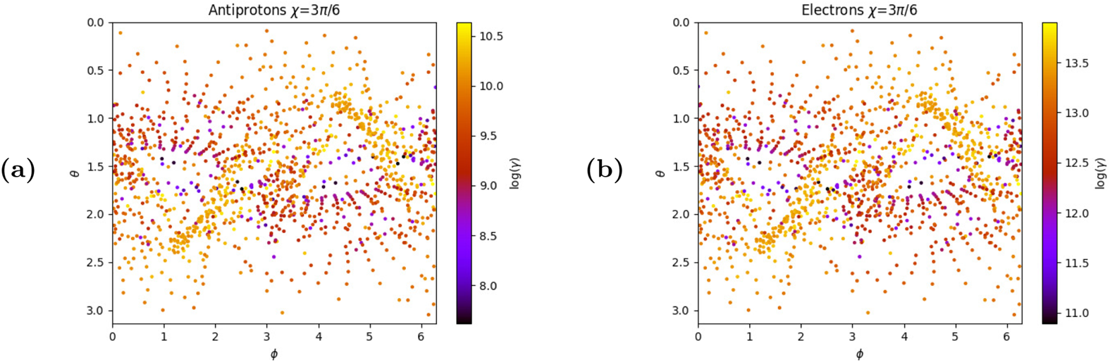
The same trajectory of antiprotons and electrons, despite their mass difference, is visible in figure 12. Our guess is that the magnetic field is so strong that particles are forced to follow the same magnetic field lines and only a low charge to mass ratio particle could have a different trajectory since it would be accelerated less efficiently and take more time to reach a speed close to  $c$.
Ejection maps of antiprotons (a) and electrons (b) for  $\chi =90^{\circ }$. Regular pattern placement.

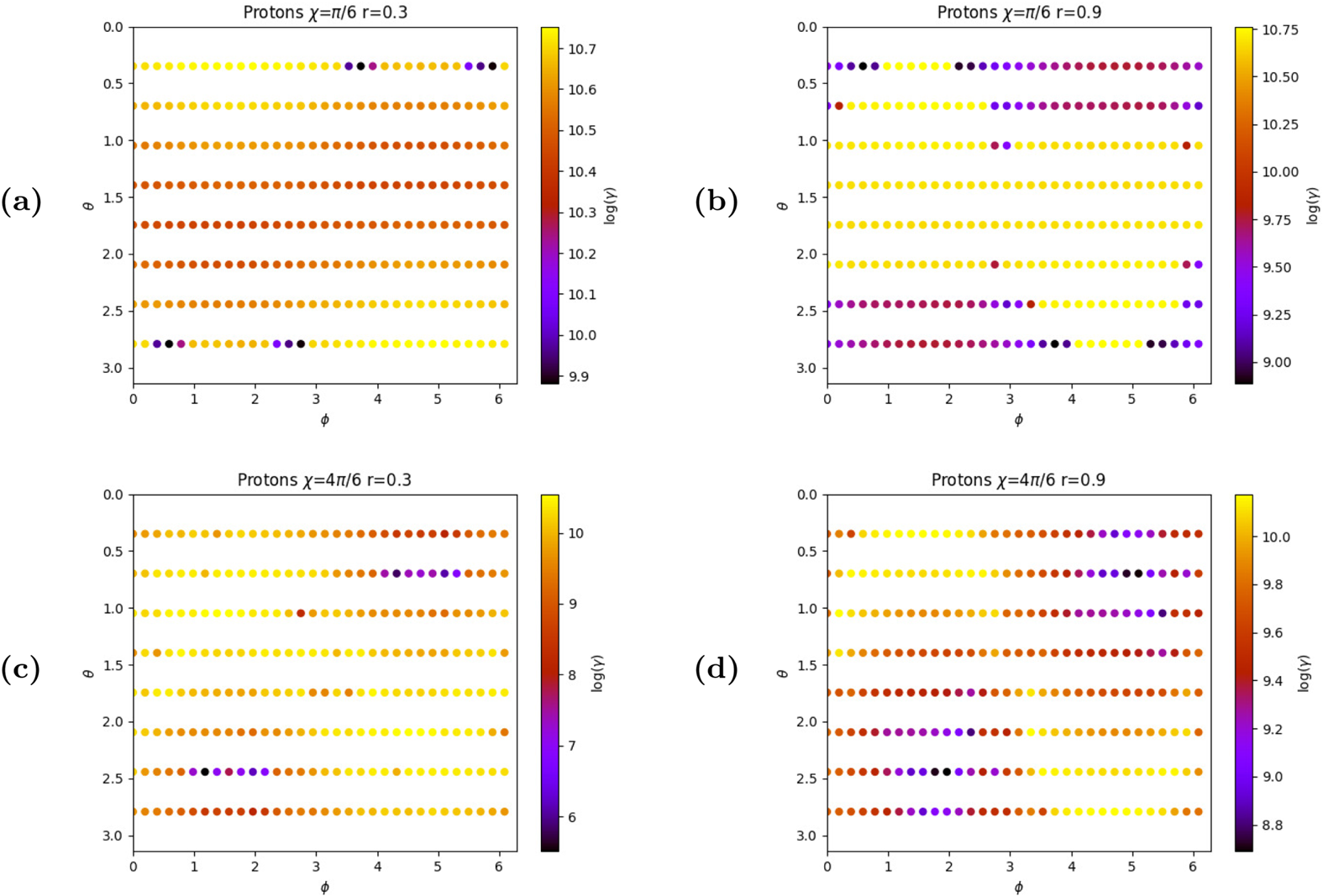
In addition, plotting the Lorentz factor map of the particles depending on their initial position shows that some areas are more prone to particle acceleration and that these regions are not randomly distributed and follow well a central symmetry, see figure 13. These maps highlighted, however, some issues, since a few particles did not follow exactly the central symmetry, meaning that, computationally speaking, some errors tend to appear during the simulations.
Final Lorentz factor of the protons depending on their initial positions, for several pulsar inclinations and a given radius of injection of the particles: (a)  $r_0=0.3r_{L}$,
 $\chi =30^{\circ }$, (b)
 $r_0=0.9r_{L}$,
 $\chi =30^{\circ }$, (c)
 $r_0=0.3r_{L}$,
 $\chi =120^{\circ }$, (d)
 $r_0=0.9r_{L}$,
 $\chi =120^{\circ }$.

Finally, aside from the case where  $\chi =90^{\circ }$, only particles with a charge of a given sign could fall onto the neutron star. Indeed, particles with positive charge crashed for
 $0^{\circ } \leq \chi \leq 90^{\circ }$ and those with negative charge for
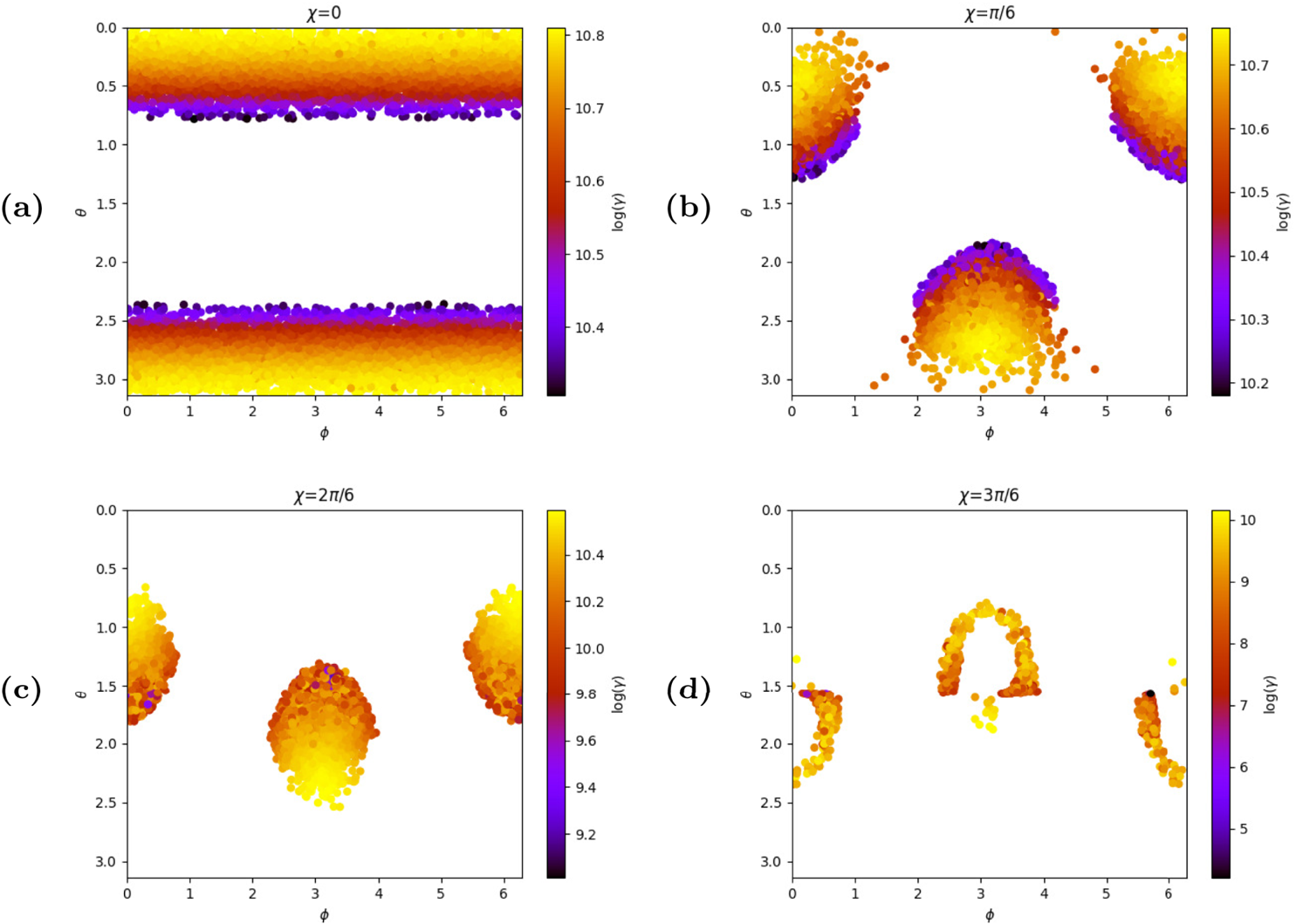
 $90^{\circ }, \leq \chi \leq 180^{\circ }$. When investigating their final coordinates, and taking into account the delay between the start of the simulation and the time the particles hit the surface, the impact maps show that the particles form hotspots around the magnetic axis instead of randomly hitting the surface, as figure 14 shows.
Impact maps of protons on the neutron star surface for  $\chi =0^{\circ }$ (a),
 $\chi =30^{\circ }$ (b),
 $\chi =60^{\circ }$ (c) and
 $\chi =90^{\circ }$ (d). Regular placement of particles.

5.4 Randomly placed particles
5.4.1 Lorentz factor of the particles
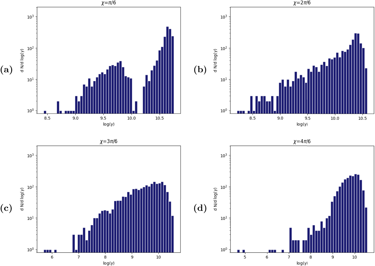
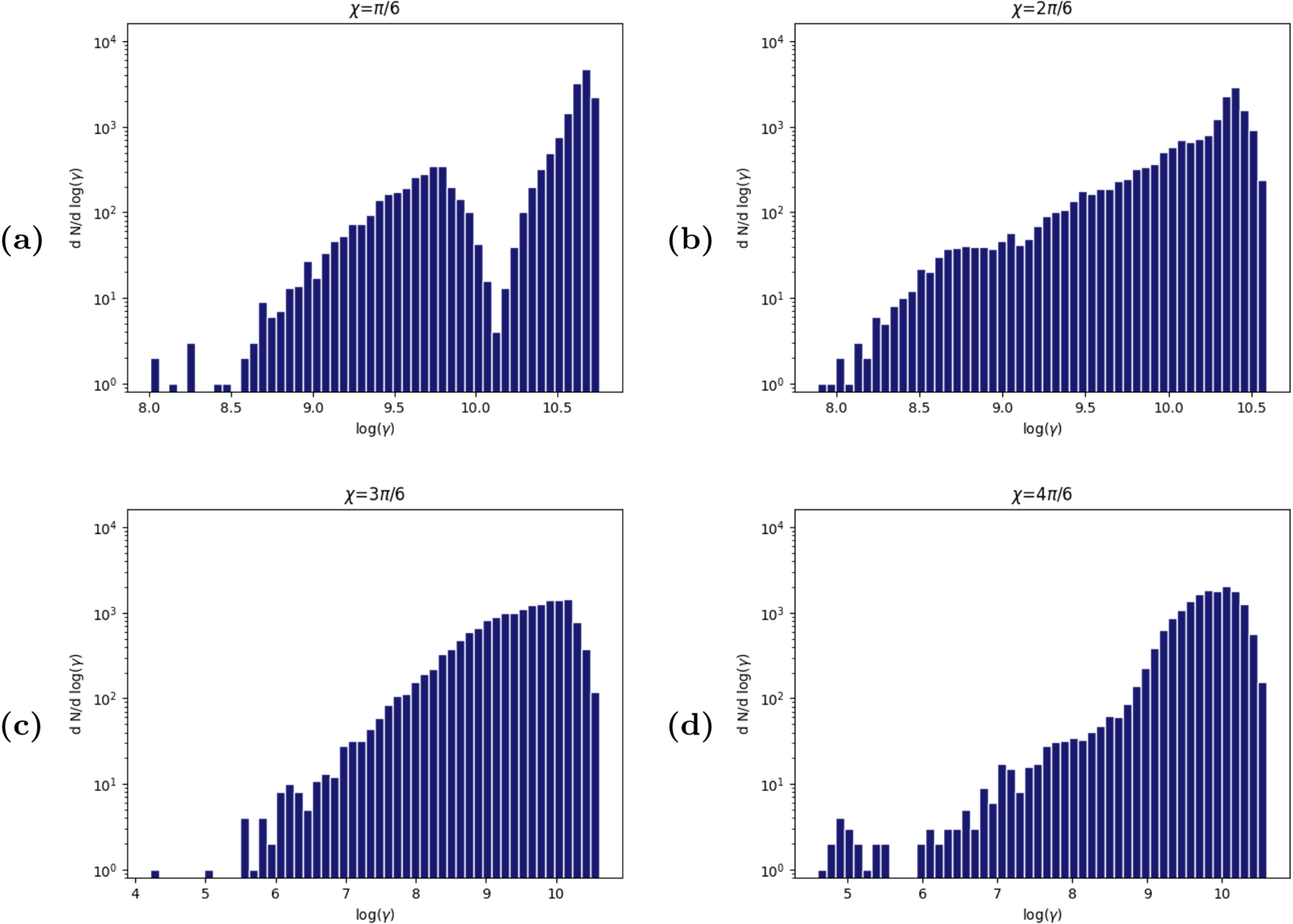
The simulations with randomly placed particles were useful for the spectral analysis, complementing those of 5.3.2. Indeed, figure 15(a) allows us to get rid of the ‘gap’ in the high energy lobe that is visible otherwise in figure 10(b) while keeping the two distinct lobes. Otherwise, the overall tendencies of the spectra were those discussed in 5.3.2. A deeper analysis with more particles yields the results shown in figure 16 with even smoother spectra and filling more the low energy end of the spectra.
Comparison of the distribution functions for 2.048 protons following the random placement: (a)  $\chi =30^{\circ }$, (b)
 $\chi =60^{\circ }$, (c)
 $\chi =90^{\circ }$, (d)
 $\chi =120^{\circ }$.

Comparison of the distribution functions for 16.384 protons following the random placement: (a)  $\chi =30^{\circ }$, (b)
 $\chi =60^{\circ }$, (c)
 $\chi =90^{\circ }$, (d)
 $\chi =120^{\circ }$.

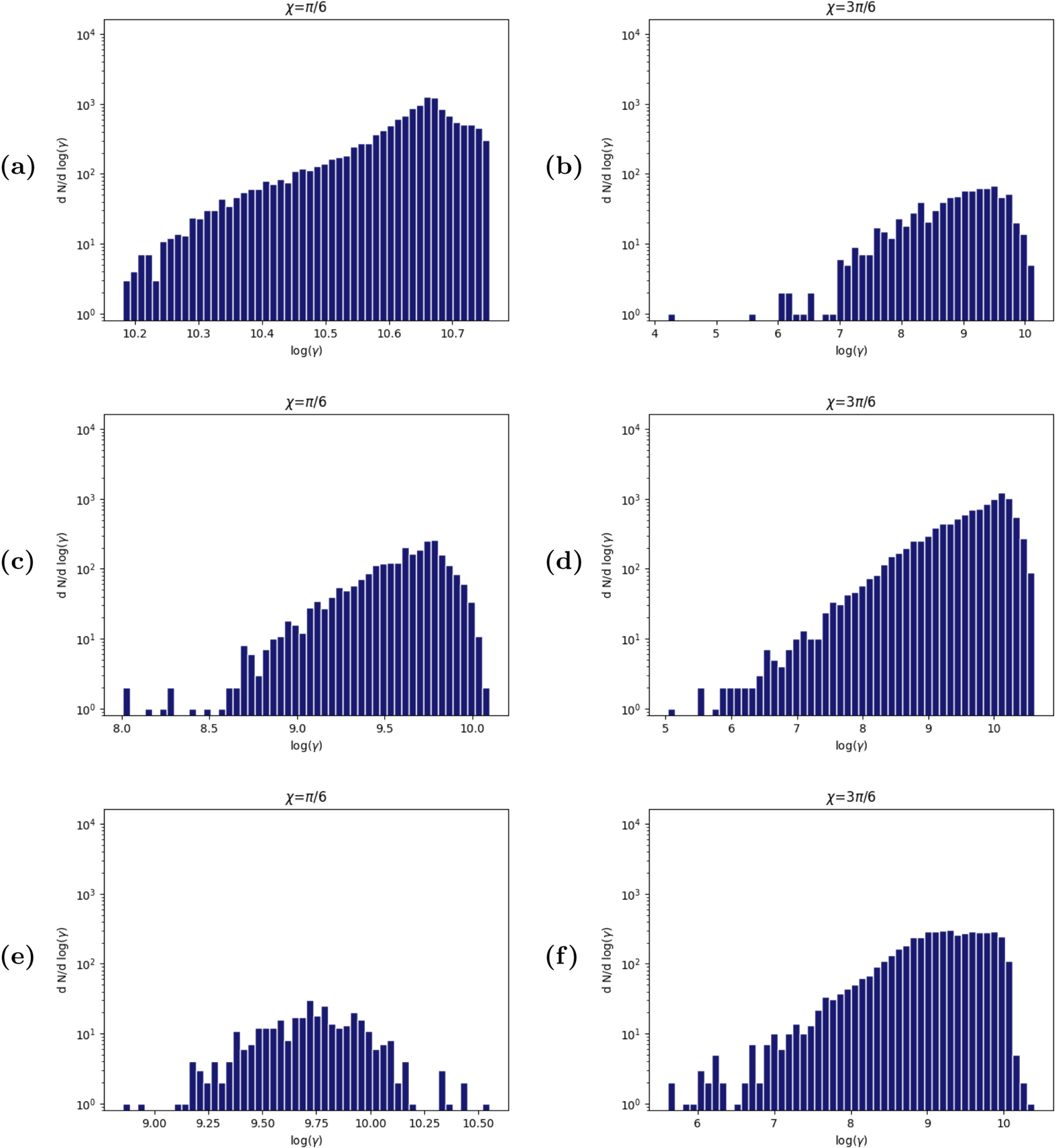
In a similar way, comparing figures 17 and 11 shows that, randomly placed particles tend to fill some of the gaps while also smoothing the distribution.And again, a higher number of particles tends to smooth the spectra, and the effect is even more noticeable on the spectra with low statistics, as shown in figure 18.
Proton distribution functions depending on their final state. (a) Crashed,  $\chi =30^{\circ }$, (b) crashed,
 $\chi =90^{\circ }$, (c) ejected,
 $\chi =30^{\circ }$, (d) ejected,
 $\chi =90^{\circ }$, (e) trapped,
 $\chi =30^{\circ }$, (f) trapped,
 $\chi =90^{\circ }$, for a random distribution of 2.048 particles.

Proton distribution functions depending on their final state. (a) Crashed,  $\chi =30^{\circ }$, (b) crashed,
 $\chi =90^{\circ }$, (c) ejected,
 $\chi =30^{\circ }$, (d) ejected,
 $\chi =90^{\circ }$, (e) trapped,
 $\chi =30^{\circ }$, (f) trapped,
 $\chi =90^{\circ }$, for a random distribution of 16.384 particles.

5.4.2 Final positions of the randomly placed particles
The simulations with 16.384 randomly placed particles still highlight over-densities and under-densities in the ejection maps. In addition, some structures where the particles have similar Lorentz factors still appear. In fact, figure 19 shows preferred directions for a given range of energy of particles.
Ejection maps for 16.384 protons following the random placement: (a)  $\chi =30^{\circ }$, (b)
 $\chi =60^{\circ }$, (c)
 $\chi =90^{\circ }$, (d)
 $\chi =120^{\circ }$.

In figure 20, impact positions are similar to those in figure 14, still with gradients of energy depending of the position of impact. Interestingly, the hotspots for  $\chi =90^{\circ }$ are still crescent shaped.
Impact maps of randomly placed protons on the neutron star surface for 16.384 particles, with  $\chi =0^{\circ }$ (a),
 $\chi =30^{\circ }$ (b),
 $\chi =60^{\circ }$ (c) and
 $\chi =90^{\circ }$ (d).

5.5 Aligned and anti-aligned neutron stars
A neutron star is aligned (respectively anti-aligned) when  $\chi =0^{\circ }$ (respectively
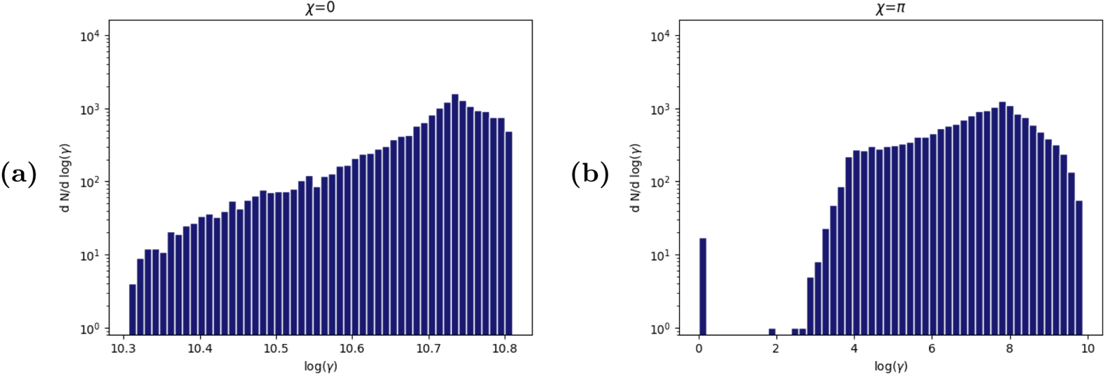
 $\chi =180^{\circ }$). In these cases, it is easier to interpret the trajectories of particles. For protons near an aligned neutron star, the poles of the star are negatively charged while the equator is positively charged. This leads the protons to be pushed away from the equator and pulled by the poles. However, even if the magnetic field is strong enough, particles still reach the poles by following the field lines, allowing them to crash easily, and since as particles get closer to the surface the electric field gets more intense, they reach an even higher Lorentz factor as proven by figure 21(a).
Spectra of protons in the aligned (a) and anti-aligned (b) cases; 2.048 protons placed in a regular pattern.

Inversely, protons around an anti-aligned neutron stars will mostly be trapped around it since they are pulled toward the equator, which is now negatively charged, but they cannot reach it due to the too strong magnetic field. These protons will feel an electric drift similar to that in figure 2 but this drift forces them to rotate around the neutron star, leading to a high spread in Lorentz factors in figure 21(b).
And with 16.384 randomly placed particles, the spectra appear to be more continuous and a peak not visible in figure 21 appears, as shown in figure 22, while keeping the same maximum Lorentz factor.
Spectra of 16.384 randomly placed protons in the aligned (a) and anti-aligned (b) cases.

6 Conclusion
In this paper, we proved that our new algorithm to simulate particles acceleration in realistic ultra-strong neutron star electromagnetic fields is efficient and accurate. We placed a constraint on the highest Lorentz factors that charged particles can reach thanks to our preliminary idealized model of a rotating magnet in vacuum.
Interestingly, the maximum Lorentz factors attainable by the particles scale linearly with their charge to mass ratio  $q/m$. The code also retrieved two expected symmetries: a charge–latitude symmetry and a central symmetry relative to the centre of the pulsar. The inclination of the pulsar has an influence on the particle distribution functions and on their final positions. Actually, positive charges hit the surface of the neutron star only for
 $\chi \leq 90^{\circ }$.
This preliminary work is encouraging but still not straightforwardly applicable per se to real neutron star electrodynamics. Nevertheless, we will pursue our effort by studying the acceleration efficiency in a plasma filled magnetosphere, which is a more realistic case than the Deutsch vacuum field. Good starting points would be resistive magnetospheres (Li et al. Reference Li, Spitkovsky and Tchekhovskoy2012) as well as radiative magnetospheres (Pétri Reference Pétri2020a,Reference Pétrib).
Because of the very high Lorentz factors, radiation reaction cannot be ignored, as shown by Laue & Thielheim (Reference Laue and Thielheim1986). We plan to add this damped motion in an upcoming work. Our long standing goal is to inject particle due to pair creation and to implement the pusher into a PIC or Vlasov code to fully and self-consistently simulate a pulsar magnetosphere with ultra-strong fields, generating current sheets and acceleration gaps. We expect a decrease of the Lorentz factors by several orders of magnitude compared to the present investigation thanks to the screening of the field and the energy lost via radiation. Our long term goal is to obtain a kinetic solution for realistic pulsar magnetospheres. The feasibility of a PIC code implementing our analytical pusher has been shown by Pétri (Reference Pétri2020c) who designed a one-dimensional relativistic electromagnetic PIC code to simulate plasma oscillations, the relativistic two-stream instability and a strongly magnetized ultra-relativistic shock. We found there that the computational cost remains manageable, with only a small overhead compared for instance with the fully implicit scheme presented by Pétri (Reference Pétri2017) and Vay (Reference Vay2008). The additional costs to boost particles and rotate the coordinate axes are largely compensated by the ability to compute realistic trajectories in ultra-strong fields.
Acknowledgements
We are grateful to the referees for helpful comments and suggestions. This work has been supported by CEFIPRA grant IFC/F5904-B/2018. We also acknowledge the High Performance Computing centre of the University of Strasbourg for supporting this work by providing scientific support and access to computing resources. Part of the computing resources were funded by the Equipex Equip@Meso project (Programme Investissements d'Avenir) and the CPER Alsacalcul/Big Data.
Editor Giovanni Manfredi thanks the referees for their advice in evaluating this article.