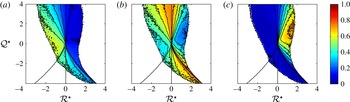
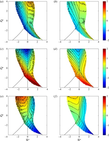
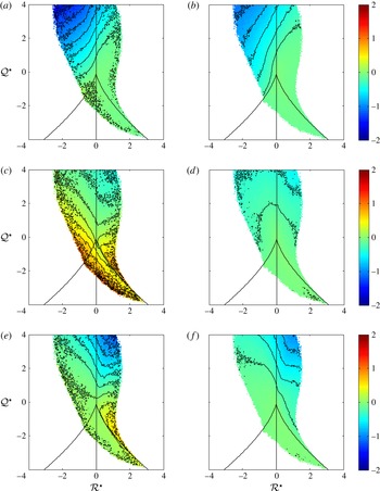
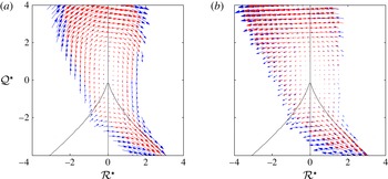
1. Introduction
The statistics of velocity gradients are very closely associated with the fine-scale motion in turbulent flows and have been well characterised in the past few decades (Wallace Reference Wallace2009). Their study is of practical interest, since velocity gradients directly influence phenomena such as flame extinction (Sreenivasan & Antonia Reference Sreenivasan and Antonia1997; Sreenivasan Reference Sreenivasan2004), the clustering of particles (Chun et al.
Reference Chun, Koch, Rani, Ahluwalia and Collins2005), and cloud formation (Bodenschatz et al.
Reference Bodenschatz, Malinowski, Shaw and Stratmann2010), cavitation (Meneveau Reference Meneveau2011) and mixing (Pumir Reference Pumir1994). From a theoretical standpoint, a theory of the fine scales of turbulent motion has perhaps the best prospect of being universal (Sreenivasan & Antonia Reference Sreenivasan and Antonia1997). Indeed, a handful of features have already been observed frequently enough for suggestion to be made that they are universal (Tsinober Reference Tsinober2009; Elsinga & Marusic Reference Elsinga and Marusic2010b
; Cardesa et al.
Reference Cardesa, Mistry, Gan and Dawson2013; Rabey, Wynn & Buxton Reference Rabey, Wynn and Buxton2015). These include: the preferential alignment of the vorticity vector with the intermediate strain eigenvector; the tendency of its associated eigenvalue to be positive on average; the ‘tearing-drop’ shape of the joint probability density function (p.d.f.) of velocity gradient tensor (VGT) invariants
 $Q=-\text{Tr}(\unicode[STIX]{x1D63C}^{2})/2$
and
 $R=-\text{Tr}(\unicode[STIX]{x1D63C}^{3})/3$
; and the ‘teapot’ shape for their counterparts in the reduced VGT. They are all obtained from single-time, single-point statistics of
 $\unicode[STIX]{x1D63C}$
.
The enstrophy and strain fields are widely reported to possess structure (Wallace Reference Wallace2009), which is presently taken to mean spatially organised regions of enstrophy and strain, correlated over large length scales. The enstrophy field tends to contain concentrated regions of high enstrophy known as ‘turbulence worms’ (She, Jackson & Orszag Reference She, Jackson and Orszag1991; Vincent & Meneguzzi Reference Vincent and Meneguzzi1991), whose radii are of the order of the Kolmogorov scale (Jiménez et al. Reference Jiménez, Wray, Saffman and Rogallo1993; Jiménez & Wray Reference Jiménez and Wray1998). They tend to cluster together (Moisy & Jiménez Reference Moisy and Jiménez2004; Leung, Swaminathan & Davidson Reference Leung, Swaminathan and Davidson2012) and are found near regions of strong dissipation (Kerr Reference Kerr1985; Vincent & Meneguzzi Reference Vincent and Meneguzzi1994; Ganapathisubramani, Lakshminarasimhan & Clemens Reference Ganapathisubramani, Lakshminarasimhan and Clemens2008; Worth & Nickels Reference Worth and Nickels2011). Regions of high dissipation tend to be organised as sheet- or ribbon-like regions (Moisy & Jiménez Reference Moisy and Jiménez2004; Ganapathisubramani et al. Reference Ganapathisubramani, Lakshminarasimhan and Clemens2008; Bermejo-Moreno, Pullin & Horiuti Reference Bermejo-Moreno, Pullin and Horiuti2009) whose dimensions are also of the order of the Kolmogorov scale and are found in the vicinity of intense vortical structures. These studies represent just a cross-section of a rather popular debate; Nelkin (Reference Nelkin1994), Bonnet & Delville (Reference Bonnet and Delville2001) and Alfonsi (Reference Alfonsi2006) provide relevant reviews.
When one considers how the velocity gradient evolves following a fluid parcel, the influence of nearby structure is felt through the pressure field: specifically, through pressure curvature, manifest by the pressure Hessian
 ${\it\Pi}_{ij}\equiv \partial ^{2}p/\partial x_{i}\partial x_{j}$
. This acts in conjunction with viscous and nonlinear effects. The nonlinear effects are purely local, i.e. they may be expressed in terms of the velocity gradient at a point. This definition treats the strain tensor as a local quantity, although it is more commonly treated as a non-local quantity. The link to structure arises because the Poisson equation for the pressure field has a source term in
 $Q$
, which may be expressed as a competition between enstrophy and strain.
There are a number of studies that examine the role of the pressure Hessian in velocity gradient dynamics (Martin et al. Reference Martin, Ooi, Chong and Soria1998; Nomura & Post Reference Nomura and Post1998; Ooi et al. Reference Ooi, Martin, Soria and Chong1999; Lüthi, Holzner & Tsinober Reference Lüthi, Holzner and Tsinober2009; Suman & Girimaji Reference Suman and Girimaji2013). Generally speaking, the pressure Hessian term acts to counteract the nonlinearity of the local term. It tends to oppose the self-amplification of strain caused by local effects and tends to oppose the locally induced reorientation of the vorticity vector with respect to the principal strain axes. Its magnitude is similar to that of local effects, so it cannot be overlooked (Martin et al. Reference Martin, Ooi, Chong and Soria1998).
Relatively few studies have examined the association of the pressure Hessian with structure. In inviscid flows, the vorticity vector tends to become a simultaneous eigenvector of the strain and pressure Hessian tensors, which is associated with stretched vortex tubes and possible blowup (Ohkitani Reference Ohkitani1993; Ohkitani & Kishiba Reference Ohkitani and Kishiba1995). In a decaying Navier–Stokes turbulence, Nomura & Post (Reference Nomura and Post1998) observed that, for regions of rotation-dominated flow, there was a similar tendency for alignment of the vorticity with the eigenvector of the pressure Hessian, which was associated with the tube-like nature of these regions; no particular structure was associated with the strain-dominated regions. These observations are a rather coarse categorisation of the behaviour and have relied upon qualitative examination of the most readily discernible, rotation-dominated, high-intensity events. Furthermore, given the computational limitations of the time, their study was at very low Reynolds number (
 $Re_{{\it\lambda}}\simeq 50$
, decaying to 25). Hence, there is scope for a broader, more detailed examination of this association at higher Reynolds numbers.
Much effort has been expended in developing models for the dynamics of velocity gradients. This is desirable for both theoretical and practical reasons: for example, better closures may lead to an improved understanding of fine-scale structure and intermittency, or the formulation of subgrid models for large-eddy simulation (Meneveau Reference Meneveau2011). Specifically, the closure of the pressure Hessian term remains a significant challenge. Only a few models explicitly incorporate the non-locality of the pressure Hessian (Chevillard et al. Reference Chevillard, Lévêque, Taddia, Meneveau, Yu and Rosales2011; Wilczek & Meneveau Reference Wilczek and Meneveau2014): most are based upon different phenomenological arguments. This is perhaps surprising, since much has been written on the role of the pressure Hessian in velocity gradient dynamics and the nature of fine-scale structure has been well characterised.
Recently, Wilczek & Meneveau (Reference Wilczek and Meneveau2014) developed a closure based on the statistics of random Gaussian fields. Their approach was to solve the transport equation for the p.d.f. of
 $\unicode[STIX]{x1D63C}$
. This approach requires closure for the mean pressure Hessian conditioned upon
 $\unicode[STIX]{x1D63C}$
, which was found from conditional averages of the
 $Q$
field, i.e. the mean distribution of
 $Q$
about a conditioning point. This led to an implicitly reversible closure with three prescribed coefficients. Since closure with the exact values for a Gaussian field led to a divergent system, the authors retained the same functional form for their closure, but chose a different set of coefficients based on direct numerical simulation (DNS) data, which yielded stationary statistics. They dubbed this the enhanced Gaussian closure (EGC). The EGC managed to qualitatively replicate a number of phenomena, including the preference for sheet-forming strain, preferred alignments of vorticity and the tearing-drop shape of the joint p.d.f. of
 $Q$
and
 $R$
. With regard to improving the model, it is not clear how well its functional form approximates real turbulence. Further, the method used to choose the coefficients failed to make explicit connection to the fine-scale structure, and it is not known whether the coefficients they found are the same in other flows.
The p.d.f. approach adopted by Girimaji & Pope (Reference Girimaji and Pope1990) and later by Wilczek & Meneveau (Reference Wilczek and Meneveau2014) shows that, as far as single-point, single-time statistics of velocity gradients are concerned, one does not need to study the full gamut of turbulent structure: just conditional structure is sufficient to capture the statistics. This provides the motivation for the present study. By examining conditional averages of the
 $Q$
field, conditioned upon
 $\unicode[STIX]{x1D63C}$
, contributions can be made to two debates. The first concerns the modelling aspect, where better models of the pressure Hessian are needed. The second concerns the link between structure and velocity gradient dynamics, where there is scope for elaboration.
In this paper, such conditional averages are examined using two complementary methods. The first approach is to approximate the mean
 $Q$
field about a point, conditional upon
 $\unicode[STIX]{x1D63C}$
at that point, using stochastic estimation (Adrian Reference Adrian1994). This approach leads to an alternative derivation of the EGC, but has the advantage that its closure coefficients are well defined and reproducible, and it explicitly reveals the kinematic features of the enstrophy and strain fields which are responsible for the dynamics. The second approach is to examine conditional averages of
 $Q$
based on just part of the information available in
 $\unicode[STIX]{x1D63C}$
, by considering conditional averages in a frame of reference defined by
 $\unicode[STIX]{x1D63C}$
. This allows us to validate the stochastic estimation method, explore where and how it fails, and give a more complete, structural explanation for a number of statistics of the pressure Hessian.
The paper is organised as follows. First, § 2.1 provides a review of velocity gradient dynamics, before discussion moves to stochastic estimation (§ 2.2) and the conditional averaging technique (§ 2.4). The methodology is concluded with a discussion of the two datasets and details of processing (§ 3). The first results are featured in § 4.1, which compares the structure identified in the turbulence data to a random Gaussian velocity field. In § 4.2 the conditional structure educed by both techniques is compared, which leads to a discussion of the implications for alignment statistics (§ 4.3) and velocity gradient dynamics (§ 4.4).
2. Methodology
2.1. Velocity gradient dynamics
To see how fine-scale structure influences velocity gradient dynamics, it is helpful to consider the transport equation (2.1) for the velocity gradient tensor, where the material derivative
 $\text{D}/\text{D}t$
is represented with an overdot (for a nice exposition of the topic, see Cantwell (Reference Cantwell1992) or Wilczek & Meneveau (Reference Wilczek and Meneveau2014)):
 $$\begin{eqnarray}\dot{\unicode[STIX]{x1D63C}}\equiv \frac{\text{D}\unicode[STIX]{x1D63C}}{\text{D}t}=-\unicode[STIX]{x1D63C}^{2}-{\it\bf\Pi}+{\it\nu}{\rm\nabla}^{2}\unicode[STIX]{x1D63C}.\end{eqnarray}$$
The first and third terms on the right-hand side of (2.1) represent local and viscous effects, respectively. The pressure Hessian term
 ${\it\Pi}_{ij}\equiv \partial ^{2}p/\partial x_{i}\partial x_{j}$
represents the influence of non-local effects via the pressure field. Since the pressure field must maintain incompressibility (
 $\boldsymbol{{\rm\nabla}}\boldsymbol{\cdot }\boldsymbol{u}=0$
), it is related to
 $\unicode[STIX]{x1D63C}$
through a Poisson equation
 $$\begin{eqnarray}{\rm\nabla}^{2}p=\text{Tr}({\it\bf\Pi})=-\text{Tr}(\unicode[STIX]{x1D63C}^{2})=2Q={\it\omega}^{2}/2-s^{2},\end{eqnarray}$$
where
 $s^{2}$
and
 ${\it\omega}^{2}$
are the total strain and enstrophy. This leads to a common decomposition of
 ${\it\bf\Pi}$
into the sum of isotropic and deviatoric parts:
 $$\begin{eqnarray}{\it\bf\Pi}=-\frac{\unicode[STIX]{x1D644}}{3}\text{Tr}(\unicode[STIX]{x1D63C}^{2})+\unicode[STIX]{x1D643}.\end{eqnarray}$$
Equation (2.2) shows the non-local dependence of the pressure field upon the spatial distribution of
 $Q$
and thus the distribution of enstrophy and strain. The deviatoric pressure Hessian
 $\unicode[STIX]{x1D643}$
is purely non-local and its explicit dependence at
 $\boldsymbol{x}$
upon the surrounding distribution of
 $Q^{\prime }=Q(\boldsymbol{x}+\boldsymbol{r})$
can be expressed via a weighted volume integral (Ohkitani & Kishiba Reference Ohkitani and Kishiba1995),
 $$\begin{eqnarray}H_{ij}(\boldsymbol{x})=\iiint \frac{{\it\delta}_{ij}-3\hat{r}_{i}\hat{r}_{j}}{2{\rm\pi}r^{3}}Q^{\prime }\,\text{d}\boldsymbol{r},\end{eqnarray}$$
where
 $\boldsymbol{r}=r\hat{\boldsymbol{r}}$
and the integral is taken in the Cauchy principal value sense over all space (excluding
 $r=0$
). It is immediately apparent that the most proximate features of the flow field have the greatest influence over the pressure Hessian at any given point.
A little more insight can be extracted from (2.1) by considering the evolution of the strain
 $\unicode[STIX]{x1D64E}$
(2.5) and vorticity
 ${\bf\omega}$
(2.7), representing the symmetric (
 $\unicode[STIX]{x1D64E}$
) and antisymmetric (
 $\unicode[STIX]{x1D652}$
) parts of
 $\unicode[STIX]{x1D63C}$
. Whilst the evolution of strain (2.5) is influenced by viscous, non-local (2.4) and local effects (represented by
 $\unicode[STIX]{x1D647}$
, (2.6)), only local (vortex stretching) and viscous effects determine the evolution of vorticity (2.7). Thus, non-local effects directly influence velocity gradients through interaction with the strain field, which subsequently interacts with the vorticity field. Furthermore, in this decomposition, each term individually satisfies the incompressibility criterion, as every term has zero trace:
 $$\begin{eqnarray}\displaystyle & \dot{\unicode[STIX]{x1D64E}}=-\unicode[STIX]{x1D647}-\unicode[STIX]{x1D643}+{\it\nu}{\rm\nabla}^{2}\unicode[STIX]{x1D64E}, & \displaystyle\end{eqnarray}$$
 $$\begin{eqnarray}\displaystyle & \unicode[STIX]{x1D647}=\left(\displaystyle \unicode[STIX]{x1D64E}^{2}-\frac{\unicode[STIX]{x1D644}}{3}\text{Tr}(\unicode[STIX]{x1D64E}^{2})\right)+\left(\displaystyle \unicode[STIX]{x1D652}^{2}-\frac{\unicode[STIX]{x1D644}}{3}\text{Tr}(\unicode[STIX]{x1D652}^{2})\right), & \displaystyle\end{eqnarray}$$
 $$\begin{eqnarray}\displaystyle & \dot{{\bf\omega}}=\unicode[STIX]{x1D64E}{\bf\omega}+{\it\nu}{\rm\nabla}^{2}{\bf\omega}. & \displaystyle\end{eqnarray}$$
She et al. (Reference She, Jackson and Orszag1991) provided further insight into this dynamical system by examining the transport equations for
 $\unicode[STIX]{x1D63C}$
in a frame of reference aligned with the eigenvectors
 $\boldsymbol{e}_{i}$
of the strain-rate tensor
 $\unicode[STIX]{x1D64E}$
, whose associated eigenvalues
 ${\it\sigma}_{i}$
are ordered
 ${\it\sigma}_{1}\geqslant {\it\sigma}_{2}\geqslant {\it\sigma}_{3}$
, with incompressibility (
 $\text{Tr}(\unicode[STIX]{x1D64E})=0$
) implying
 ${\it\sigma}_{1}\geqslant 0$
and
 ${\it\sigma}_{3}\leqslant 0$
. Quantities evaluated in the strain basis are denoted with a tilde; the velocity gradient tensor simplifies to
 $$\begin{eqnarray}\widetilde{\unicode[STIX]{x1D63C}}=\left[\begin{array}{@{}ccc@{}}{\it\sigma}_{1} & -\widetilde{{\it\omega}}_{3}/2 & \widetilde{{\it\omega}}_{2}/2\\ \widetilde{{\it\omega}}_{3}/2 & {\it\sigma}_{2} & -\widetilde{{\it\omega}}_{1}/2\\ -\widetilde{{\it\omega}}_{2}/2 & \widetilde{{\it\omega}}_{1}/2 & {\it\sigma}_{3}\end{array}\right],\end{eqnarray}$$
whilst local strain production
 $\widetilde{\unicode[STIX]{x1D647}}$
becomes
 $$\begin{eqnarray}\widetilde{\unicode[STIX]{x1D647}}=\left[\begin{array}{@{}ccc@{}}{\it\sigma}_{1}^{2}-s^{2}/3 & 0 & 0\\ 0 & {\it\sigma}_{2}^{2}-s^{2}/3 & 0\\ 0 & 0 & {\it\sigma}_{3}^{2}-s^{2}/3\end{array}\right]+\frac{1}{4}\left[\begin{array}{@{}ccc@{}}\widetilde{{\it\omega}}_{1}^{2}-{\it\omega}^{2}/3 & \widetilde{{\it\omega}}_{1}\widetilde{{\it\omega}}_{2} & \widetilde{{\it\omega}}_{1}\widetilde{{\it\omega}}_{3}\\ \widetilde{{\it\omega}}_{1}\widetilde{{\it\omega}}_{2} & \widetilde{{\it\omega}}_{2}^{2}-{\it\omega}^{2}/3 & \widetilde{{\it\omega}}_{2}\widetilde{{\it\omega}}_{3}\\ \widetilde{{\it\omega}}_{1}\widetilde{{\it\omega}}_{3} & \widetilde{{\it\omega}}_{2}\widetilde{{\it\omega}}_{3} & \widetilde{{\it\omega}}_{3}^{2}-{\it\omega}^{2}/3\end{array}\right]\!.\end{eqnarray}$$
The familiar transport equation for vorticity gains an extra term (2.11), which incorporates the fact that the reference frame is rotating (2.12). The diagonal entries of
 $\widetilde{\unicode[STIX]{x1D643}}$
are responsible for the (non-local) generation of principal strain (2.10) and the off-diagonals rotate the reference frame, as does a misalignment of the vorticity with the principal axes (2.12):
 $$\begin{eqnarray}\displaystyle & \dot{{\it\sigma}}_{i}=-\widetilde{L}_{ii}-\widetilde{H}_{ii}+{\it\nu}{\rm\nabla}^{2}{\it\sigma}_{i}, & \displaystyle\end{eqnarray}$$
 $$\begin{eqnarray}\displaystyle & \dot{\widetilde{{\it\omega}}}_{i}=\displaystyle {\it\sigma}_{i}\widetilde{{\it\omega}}_{i}+\mathop{\sum }_{j\neq i}\frac{\widetilde{L}_{ij}+\widetilde{H}_{ij}}{{\it\sigma}_{j}-{\it\sigma}_{i}}\widetilde{{\it\omega}}_{j}+{\it\nu}{\rm\nabla}^{2}\widetilde{{\it\omega}}_{i}, & \displaystyle\end{eqnarray}$$
 $$\begin{eqnarray}\displaystyle & \dot{\boldsymbol{e}}_{i}\boldsymbol{\cdot }\boldsymbol{e}_{j}=\displaystyle \frac{\widetilde{L}_{ij}+\widetilde{H}_{ij}}{{\it\sigma}_{j}-{\it\sigma}_{i}}+{\it\nu}({\rm\nabla}^{2}\boldsymbol{e}_{i})\boldsymbol{\cdot }\boldsymbol{e}_{j}. & \displaystyle\end{eqnarray}$$
The single-point, single-time statistics of
 $\unicode[STIX]{x1D63C}$
can be completely described by its p.d.f., defined as
 $P_{\unicode[STIX]{x1D63C}}({\mathcal{A}};t)\equiv \langle {\it\delta}(\unicode[STIX]{x1D63C}(\boldsymbol{x},t)-{\mathcal{A}})\rangle$
, where
 ${\mathcal{A}}$
is the sample space variable of
 $\unicode[STIX]{x1D63C}$
at point
 $\boldsymbol{x}$
and time
 $t$
. Herein, calligraphic letters are used to represent sample space variables. In the absence of stochastic forcing, the p.d.f. can be shown to evolve according to (2.13) (Girimaji & Pope Reference Girimaji and Pope1990; Wilczek & Meneveau Reference Wilczek and Meneveau2014):
 $$\begin{eqnarray}\displaystyle & \displaystyle \frac{\partial P_{\unicode[STIX]{x1D63C}}({\mathcal{A}};t)}{\partial t}=-\frac{\partial }{\partial {\mathcal{A}}_{ij}}\left(\left[-\left({\mathcal{A}}_{ik}{\mathcal{A}}_{kj}-\frac{{\it\delta}_{ij}}{3}{\mathcal{A}}_{kl}{\mathcal{A}}_{lk}\right)-\langle H_{ij}|{\mathcal{A}}\rangle \right.\right. & \displaystyle \nonumber\\ \displaystyle & \displaystyle \left.\left.\hspace{70.0001pt}+\,\langle {\it\nu}{\rm\Delta}A_{ij}|{\mathcal{A}}\rangle \vphantom{\left(\frac{{\it\delta}_{ij}}{3}\right)}\right]P_{\unicode[STIX]{x1D63C}}({\mathcal{A}},t)\right)-\frac{\partial }{\partial x_{k}}\langle u_{k}{\it\delta}(\unicode[STIX]{x1D63C}(\boldsymbol{x},t)-{\mathcal{A}})\rangle . & \displaystyle\end{eqnarray}$$
The main point of reproducing (2.13) here is to point out that the influence of structure upon single-point, single-time statistics is expressed purely in terms of averages conditional upon
 $\unicode[STIX]{x1D63C}$
.
The projection in the
 $(R,Q)$
plane represents just part of the information available from
 $P_{\unicode[STIX]{x1D63C}}$
, but the remarkable reproducibility of the joint p.d.f.
 $P_{RQ}({\mathcal{R}},{\mathcal{Q}})$
makes this projection a good candidate for further simplification of velocity gradient dynamics. In a similar fashion to (2.13), one may describe the evolution of
 $P_{RQ}$
in terms of the conditional mean material derivative of
 $R$
and
 $Q$
(2.14) (Chevillard et al.
Reference Chevillard, Meneveau, Biferale and Toschi2008):
 $$\begin{eqnarray}\displaystyle \left.\begin{array}{@{}c@{}}\langle \dot{Q}|{\mathcal{R}},{\mathcal{Q}}\rangle =-3R+\langle \text{Tr}(\unicode[STIX]{x1D63C}\unicode[STIX]{x1D643})|{\mathcal{R}},{\mathcal{Q}}\rangle -{\it\nu}\langle \text{Tr}(\unicode[STIX]{x1D63C}{\rm\nabla}^{2}\unicode[STIX]{x1D63C})|{\mathcal{R}},{\mathcal{Q}}\rangle ,\\ \langle {\dot{R}}|{\mathcal{R}},{\mathcal{Q}}\rangle =-{\textstyle \frac{2}{3}}Q^{2}+\langle \text{Tr}(\unicode[STIX]{x1D63C}^{2}\unicode[STIX]{x1D643})|{\mathcal{R}},{\mathcal{Q}}\rangle -{\it\nu}\langle \text{Tr}(\unicode[STIX]{x1D63C}^{2}{\rm\nabla}^{2}\unicode[STIX]{x1D63C})|{\mathcal{R}},{\mathcal{Q}}\rangle .\end{array}\right\} & & \displaystyle\end{eqnarray}$$
The
 $(R,Q)$
phase plane dynamics has been characterised by Martin et al. (Reference Martin, Ooi, Chong and Soria1998), Ooi et al. (Reference Ooi, Martin, Soria and Chong1999) and Lüthi et al. (Reference Lüthi, Holzner and Tsinober2009) (amongst others): the general tendency is for the non-local terms (contractions of
 $\unicode[STIX]{x1D643}$
) to counteract the local terms (in
 $R$
and
 $Q^{2}$
), whilst viscosity introduces the skewed shape and acts as a damping term
For incompressible flows,
 $R$
and
 $Q$
are sufficient to categorise the local flow topology (Chong, Perry & Cantwell Reference Chong, Perry and Cantwell1990), since this is determined by the eigenvalues of
 $\unicode[STIX]{x1D63C}$
. When the discriminant
 $D=(4/27)R^{2}+Q^{3}$
is positive,
 $\unicode[STIX]{x1D63C}$
has one real and two complex eigenvalues: the corresponding pattern of streamlines in a nearby region may be a stable focus with stretching (
 $R<0$
, SF/S) or unstable focus with compression (
 $R>0$
, UF/C). When
 $D$
is negative, all eigenvalues of
 $\unicode[STIX]{x1D63C}$
are real: locally, the streamlines form a pair of saddles and either a stable (
 $R<0$
, SN/S/S) or unstable (
 $R>0$
, UN/S/S) node. Whilst
 $Q$
may be thought of as a competition between strain and enstrophy (2.2),
 $R$
may be similarly decomposed as
 $$\begin{eqnarray}R=-{\it\sigma}_{1}{\it\sigma}_{2}{\it\sigma}_{3}-{\textstyle \frac{1}{4}}{\bf\omega}^{\text{T}}\unicode[STIX]{x1D64E}{\bf\omega},\end{eqnarray}$$
which may be thought of as a balance between local production of enstrophy (by
 ${\bf\omega}^{\text{T}}\unicode[STIX]{x1D64E}{\bf\omega}$
) and strain (by
 ${\it\sigma}_{1}{\it\sigma}_{2}{\it\sigma}_{3}$
).
With regard to modelling velocity gradient dynamics, a number of works have adopted p.d.f. methods (Girimaji & Pope Reference Girimaji and Pope1990; Chevillard et al.
Reference Chevillard, Meneveau, Biferale and Toschi2008; Wilczek & Meneveau Reference Wilczek and Meneveau2014). Then, one speaks of modelling the conditional deviatoric pressure Hessian
 $\langle \unicode[STIX]{x1D643}|{\mathcal{A}}\rangle$
and viscous Laplacian
 $\langle {\rm\nabla}^{2}\unicode[STIX]{x1D63C}|{\mathcal{A}}\rangle$
. In particular, the closure of the pressure Hessian term remains one of the biggest challenges (Meneveau Reference Meneveau2011).
Recently, Wilczek & Meneveau (Reference Wilczek and Meneveau2014) took a novel approach to modelling the pressure Hessian, through a consideration of the behaviour of random Gaussian velocity fields. By obtaining an exact expression for
 $\langle Q^{\prime }|{\mathcal{A}}\rangle$
and exploiting its relation to the pressure Hessian (2.4), they found that, for the Gaussian case, the conditional deviatoric pressure Hessian
 $\langle \unicode[STIX]{x1D643}|{\mathcal{A}}\rangle$
has the form
 $$\begin{eqnarray}\widehat{\unicode[STIX]{x1D643}}={\it\alpha}^{\prime }\left({\mathcal{S}}^{2}-\frac{\unicode[STIX]{x1D644}}{3}\text{Tr}({\mathcal{S}}^{2})\right)+{\it\beta}^{\prime }\left({\mathcal{W}}^{2}-\frac{\unicode[STIX]{x1D644}}{3}\text{Tr}({\mathcal{W}}^{2})\right)+{\it\gamma}^{\prime }\left({\mathcal{S}}-{\mathcal{W}}\right),\end{eqnarray}$$
where
 ${\mathcal{S}}$
and
 ${\mathcal{W}}$
are the symmetric and antisymmetric parts of
 ${\mathcal{A}}$
and the coefficients
 ${\it\alpha}^{\prime }$
,
 ${\it\beta}^{\prime }$
and
 ${\it\gamma}^{\prime }$
are constants related to the velocity autocorrelation function. Note that, because all the terms in
 ${\mathcal{A}}$
are quadratic,
 $\widehat{\unicode[STIX]{x1D643}}$
is preserved under time reversal (
 $\unicode[STIX]{x1D63C}\rightarrow -\unicode[STIX]{x1D63C}$
).
Unfortunately, the coefficients prescribed by the Gaussian closure led to a divergent system. To remedy this, they created the EGC, which adopted the functional form of (2.16), but fitted coefficients to DNS data to satisfy (2.17):
 $$\begin{eqnarray}\left.\begin{array}{@{}c@{}}\langle \text{Tr}(\unicode[STIX]{x1D64E}\unicode[STIX]{x1D652}\unicode[STIX]{x1D643})\rangle =\langle \text{Tr}(\unicode[STIX]{x1D64E}\unicode[STIX]{x1D652}\widehat{\unicode[STIX]{x1D643}})\rangle ,\\ \langle \text{Tr}(\unicode[STIX]{x1D64E}^{2}\unicode[STIX]{x1D643})\rangle =\langle \text{Tr}(\unicode[STIX]{x1D64E}^{2}\widehat{\unicode[STIX]{x1D643}})\rangle ,\\ \langle \text{Tr}(\unicode[STIX]{x1D652}^{2}\unicode[STIX]{x1D643})\rangle =\langle \text{Tr}(\unicode[STIX]{x1D652}^{2}\widehat{\unicode[STIX]{x1D643}})\rangle .\end{array}\right\}\end{eqnarray}$$
These coefficients sufficiently reduced the nonlinearity to produce stationary statistics, which qualitatively captured the phenomena discussed above. However, the model fails under a quantitative comparison of these phenomena against the DNS data upon which it was based. It is an attractive starting point, as it has a sound mathematical basis and already considerable success.
As Wilczek & Meneveau (Reference Wilczek and Meneveau2014) point out, there are many ways to obtain the closure coefficients empirically: in § 2.2, it becomes clear that their method is equivalent to a stochastic estimation. Taking this empirical approach, one must then ask: Can the coefficients derived from their dataset be reproduced in other flows? If one looks to improve the model, then one must ask: How should the functional form of (2.16) be modified to better represent the behaviour of
 $\langle \unicode[STIX]{x1D643}|{\mathcal{A}}\rangle$
? Can some possibilities be excluded? For example: the EGC has implicit time-reversal symmetry, since odd terms in
 ${\mathcal{A}}$
are absent, which one might justify on the basis that
 $\unicode[STIX]{x1D643}$
is an even function of the velocity gradient tensor field. On the other hand, this property does not necessarily extend to the conditional average given
 ${\mathcal{A}}$
. These points are addressed in §§ 4.1 and 2.2.
The above discussion has served to introduce the fundamentals of velocity gradient dynamics. Furthermore, it has shown that structure, embodied by footprints of structure left in the conditional
 $Q$
field, may be used not only to understand velocity gradient dynamics, but also to inform their modelling.
2.2. Stochastic estimation of the conditional
 $Q$
field

In this section, a closure for
 $\langle \unicode[STIX]{x1D643}|{\mathcal{A}}\rangle$
is sought by constructing an approximation for
 $\langle Q^{\prime }|{\mathcal{A}}\rangle$
, exploiting the principle of local isotropy. This implies invariance to arbitrary rotations and reflections
 $\unicode[STIX]{x1D651}$
of the coordinate system:
 $$\begin{eqnarray}\langle Q(\boldsymbol{x}+\boldsymbol{r})|{\mathcal{A}}\rangle =\langle Q(\boldsymbol{x}+\unicode[STIX]{x1D651}\boldsymbol{r})|\unicode[STIX]{x1D651}{\mathcal{A}}\unicode[STIX]{x1D651}^{\text{T}}\rangle .\end{eqnarray}$$
Starting with a Taylor series expansion, one obtains
 $$\begin{eqnarray}\langle Q^{\prime }|{\mathcal{A}}\rangle =a(\boldsymbol{r})+b_{ij}(\boldsymbol{r}){\mathcal{A}}_{ij}+c_{ijkl}(\boldsymbol{r}){\mathcal{A}}_{ij}{\mathcal{A}}_{kl}+O({\mathcal{A}}^{3}).\end{eqnarray}$$
Retaining terms up to second order, the most general isotropic form of the approximation
 $\widehat{Q}$
is
 $$\begin{eqnarray}\displaystyle \widehat{Q}({\mathcal{A}},\boldsymbol{r}) & = & \displaystyle b_{1}{\it\tau}_{0}^{-2}+b_{2}(\hat{\boldsymbol{r}}^{\text{T}}{\mathcal{A}}\hat{\boldsymbol{r}}){\it\tau}_{0}^{-1}+b_{3}\text{Tr}({\mathcal{A}}^{2})+b_{4}\text{Tr}({\mathcal{A}}{\mathcal{A}}^{\text{T}})\nonumber\\ \displaystyle & & \displaystyle +\,b_{5}(\hat{\boldsymbol{r}}^{\text{T}}{\mathcal{A}}^{2}\hat{r})+b_{6}(\hat{\boldsymbol{r}}^{\text{T}}{\mathcal{A}}{\mathcal{A}}^{\text{T}}\hat{r})+b_{7}(\hat{\boldsymbol{r}}^{\text{T}}{\mathcal{A}}^{\text{T}}{\mathcal{A}}\hat{r})+b_{8}(\hat{\boldsymbol{r}}^{\text{T}}{\mathcal{A}}\hat{r})^{2},\end{eqnarray}$$
where the coefficient functions
 $b_{i}$
are scalar functions of
 $r$
. The time scale
 ${\it\tau}_{0}$
has been introduced to make all
 $b_{i}$
dimensionless; later, it will be shown that the Kolmogorov time scale is the appropriate time scale for this term. This strongly resembles the functional form for a Gaussian velocity field, in which
 ${\it\tau}_{0}$
is the Kolmogorov time scale and the
 $b_{2}$
term is missing. It may be expressed more compactly as
 $$\begin{eqnarray}\widehat{Q}({\mathcal{A}},\boldsymbol{r})=E_{j}({\mathcal{A}},\hat{\boldsymbol{r}})b_{j}(r),\end{eqnarray}$$
where the event vector
 $E_{j}$
is defined as
 $$\begin{eqnarray}\boldsymbol{E}=[{\it\tau}_{0}^{-2},(\hat{\boldsymbol{r}}^{\text{T}}\unicode[STIX]{x1D63C}\hat{\boldsymbol{r}}){\it\tau}_{0}^{-1}\text{Tr}(\unicode[STIX]{x1D63C}^{2}),\text{Tr}(\unicode[STIX]{x1D63C}\unicode[STIX]{x1D63C}^{\text{T}}),(\hat{\boldsymbol{r}}^{\text{T}}\unicode[STIX]{x1D63C}^{2}\hat{r}),(\hat{\boldsymbol{r}}^{\text{T}}\unicode[STIX]{x1D63C}\unicode[STIX]{x1D63C}^{\text{T}}\hat{r}),(\hat{\boldsymbol{r}}^{\text{T}}\unicode[STIX]{x1D63C}^{\text{T}}\unicode[STIX]{x1D63C}\hat{r}),(\hat{\boldsymbol{r}}^{\text{T}}\unicode[STIX]{x1D63C}\hat{r})^{2}].\end{eqnarray}$$
The choice of event vector
 $\boldsymbol{E}$
is not unique: there are infinitely many linear combinations that contain the same information. One such alternative is the permuted event vector
 $\boldsymbol{F}$
below, where each element is simply a linear combination of the elements of
 $\boldsymbol{E}$
:
 $$\begin{eqnarray}\boldsymbol{F}=\left[\begin{array}{@{}cccccccc@{}}{\it\tau}_{0}^{-2} & {\textstyle \frac{1}{2}}{\bf\omega}^{2} & {\textstyle \frac{1}{2}}({\bf\omega}\boldsymbol{\cdot }\hat{\boldsymbol{r}})^{2} & \hat{\boldsymbol{r}}^{\text{T}}\unicode[STIX]{x1D64E}\hat{\boldsymbol{r}}{\it\tau}_{0}^{-1} & s^{2} & \hat{\boldsymbol{r}}^{\text{T}}\unicode[STIX]{x1D64E}^{2}\hat{\boldsymbol{r}} & (\hat{\boldsymbol{r}}^{\text{T}}\unicode[STIX]{x1D64E}\hat{\boldsymbol{r}})^{2} & \hat{\boldsymbol{r}}^{\text{T}}(\unicode[STIX]{x1D64E}\unicode[STIX]{x1D652}-\unicode[STIX]{x1D652}\unicode[STIX]{x1D64E})\hat{\boldsymbol{r}}\end{array}\right]\!.\end{eqnarray}$$
Analogously, the expression for this basis becomes
 $\widehat{Q}(\boldsymbol{x}+\boldsymbol{r})=\unicode[STIX]{x1D60D}_{j}(\boldsymbol{x},\hat{\boldsymbol{r}})c_{j}(r)$
. This definition has a more ready physical interpretation, so the task becomes to obtain
 $c_{j}$
rather than
 $b_{j}$
. There is no material difference apart from the expression being a different combination of the terms.
Stochastic estimation (Adrian Reference Adrian1994) provides a means of obtaining
 $c_{j}(r)$
. Stochastic estimation has been applied previously to the approximation of highly complex conditional averages in turbulent flows, with great success. The basic premise is to approximate conditional averages with the first few terms of their Taylor series expansion, such that the mean-square error between the model and the conditional average is minimised.
The stochastic estimation contains eight coefficients
 $c_{j}$
, which may be adjusted independently at given radius
 $r$
. To obtain a best fit to the true conditional average, an objective function
 $G(r)$
is defined as the average over all solid angle
 ${\it\Omega}$
of the mean-square error between the conditional average and the approximation:
 $$\begin{eqnarray}G(r)=\frac{1}{4{\rm\pi}}\left\langle \iint (\widehat{Q}-\langle Q^{\prime }|{\mathcal{A}}\rangle )^{2}\,\text{d}{\it\Omega}\right\rangle .\end{eqnarray}$$
The best set of coefficients
 $c_{j}(r)$
is obtained by minimising
 $G(r)$
, which is obtained when
 $\partial G/\partial c_{j}=0$
. Thus, the chosen
 $c_{j}$
provide a model that is the best fit, in the least-squares sense, to the true conditional average. For brevity, the solid-angle average of a quantity
 ${\it\psi}(\hat{\boldsymbol{r}})$
is expressed with an overbar, i.e.
 $$\begin{eqnarray}\overline{{\it\psi}}=\frac{1}{4{\rm\pi}}\iint {\it\psi}\,\text{d}{\it\Omega},\end{eqnarray}$$
which results in
 $c_{j}$
being determined by
 $$\begin{eqnarray}\overline{\langle \unicode[STIX]{x1D60D}_{j}\unicode[STIX]{x1D60D}_{k}\rangle }c_{k}(r)=\overline{\langle Q^{\prime }\unicode[STIX]{x1D60D}_{j}\rangle }.\end{eqnarray}$$
It is worth noting that the end result is essentially a set of two-point correlation functions, obtained from a multiple variable regression analysis. Since the analysis contains all leading-order terms in the isotropic form of
 $\langle Q^{\prime }|{\mathcal{A}}\rangle$
, any confounding factors are relegated to third-order terms and above, such that examination of the coefficient functions reveals the predominant behaviour of the true conditional average.
In general, the 64 entries of the solid-angle-averaged tensor
 $\overline{\langle \unicode[STIX]{x1D60D}_{j}\unicode[STIX]{x1D60D}_{k}\rangle }$
may be expressed as some linear combination of eight independent terms (except for a multiple of
 ${\it\tau}_{0}$
), consisting of second-, third- and fourth-order moments of the velocity gradient tensor. This is because every entry is Galilean-invariant (by definition) and there are two, two and four independent, Galilean invariant, second-, third- and fourth-order moments of velocity gradients, respectively (Siggia Reference Siggia1981).
Homogeneity constrains the relation between the
 $c_{j}$
. Since
 $\langle Q\rangle =0$
everywhere in a homogeneous flow, only seven of the eight functions are independent, as substitution into (2.26) implies
 $\overline{\langle \unicode[STIX]{x1D60D}_{j}\rangle }c_{j}=0$
. The same relation can be used to simplify
 $\overline{\langle \unicode[STIX]{x1D60D}_{j}\rangle }$
, leading to (2.27),
 $$\begin{eqnarray}\frac{c_{1}}{{\it\tau}_{0}^{2}\langle {\it\omega}^{2}\rangle }+\frac{c_{2}}{2}+\frac{c_{3}}{6}+\frac{c_{5}}{2}+\frac{c_{6}}{6}+\frac{c_{7}}{15}=0,\end{eqnarray}$$
which confirms the intuition that one ought to use the Kolmogorov time scale to normalise the coefficients
 $c_{j}$
. Therefore, the coefficient functions have been calculated using
 ${\it\tau}_{0}=\langle {\it\omega}^{2}\rangle ^{-1/2}$
, as calculated directly from velocity gradients; this is the time scale used to normalise the other velocity gradient quantities presented in this paper.
In the case of isotropic turbulence, some further simplification can be made in obtaining the coefficient functions. The mean-square error
 $\langle (\widehat{Q}-\langle Q^{\prime }|{\mathcal{A}}\rangle )^{2}\rangle$
must be a scalar function of
 $r$
and therefore independent of
 $\hat{\boldsymbol{r}}$
, so solid-angle averaging is unnecessary and the necessary functions can be derived from regular two-point correlations. In the case of axisymmetric turbulence, where there is a preferential direction
 $\hat{\boldsymbol{n}}$
, the mean-square error at
 $\boldsymbol{r}$
may depend upon
 $\hat{\boldsymbol{r}}\boldsymbol{\cdot }\hat{\boldsymbol{n}}=\cos ({\it\theta})$
and
 $r$
, so solid-angle averaging can be reduced to taking a (weighted) average over all
 ${\it\theta}$
.
Equation (2.20) is combined with (2.4) to obtain the stochastic estimation of the deviatoric pressure Hessian,
 $\widehat{\unicode[STIX]{x1D643}}$
(2.28):
 $$\begin{eqnarray}\widehat{\unicode[STIX]{x1D643}}={\it\alpha}\left({\mathcal{S}}^{2}-\frac{\unicode[STIX]{x1D644}}{3}\text{Tr}({\mathcal{S}}^{2})\right)+{\it\beta}\left({\mathcal{W}}^{2}-\frac{\unicode[STIX]{x1D644}}{3}\text{Tr}({\mathcal{W}}^{2})\right)+{\it\gamma}({\mathcal{S}}-{\mathcal{W}})+\frac{{\it\delta}}{{\it\tau}_{0}}{\mathcal{S}}.\end{eqnarray}$$
Its form is similar to the EGC (2.16), but it gains an extra term associated with
 $c_{4}$
, which corresponds to the leading-order effects of irreversibility.
The coefficients
 ${\it\alpha}$
,
 ${\it\beta}$
,
 ${\it\gamma}$
and
 ${\it\delta}$
are determined explicitly by
 $$\begin{eqnarray}{\it\alpha}=-{\textstyle \frac{4}{5}}(C_{6}+{\textstyle \frac{4}{7}}C_{7}),\quad {\it\beta}=-{\textstyle \frac{8}{5}}C_{3},\quad {\it\gamma}=-{\textstyle \frac{4}{5}}C_{8},\quad {\it\delta}=-{\textstyle \frac{4}{5}}C_{4},\end{eqnarray}$$
where
 $$\begin{eqnarray}C_{j}=\lim _{{\it\epsilon}\rightarrow 0}\int _{{\it\epsilon}}^{\infty }\frac{c_{j}}{r}\,\text{d}r.\end{eqnarray}$$
These coefficients are in fact related to the method proposed by Wilczek & Meneveau (Reference Wilczek and Meneveau2014) to obtain the coefficients for the EGC (2.16). After a lengthy proof, outlined in appendix A, one can show that the two sets of coefficients are related via
 $$\begin{eqnarray}\displaystyle & {\it\alpha}^{\prime }={\it\alpha}-3\displaystyle \frac{{\it\delta}}{{\it\tau}_{0}}\frac{T_{2}(I_{2}-3I_{3})+2I_{4}T_{1}}{(I_{2}-3I_{3})^{2}-I_{1}I_{4}}, & \displaystyle\end{eqnarray}$$
 $$\begin{eqnarray}\displaystyle & {\it\beta}^{\prime }={\it\beta}-6\displaystyle \frac{{\it\delta}}{{\it\tau}_{0}}\frac{2T_{1}(I_{2}-3I_{3})+I_{1}T_{1}}{(I_{2}-3I_{3})^{2}-I_{1}I_{4}}, & \displaystyle\end{eqnarray}$$
 $$\begin{eqnarray}\displaystyle & {\it\gamma}^{\prime }={\it\gamma}, & \displaystyle\end{eqnarray}$$
 $$\begin{eqnarray}I_{1}=\langle s^{4}\rangle ,\quad I_{2}=\langle s^{2}{\it\omega}^{2}\rangle ,\quad I_{3}=\langle (\unicode[STIX]{x1D64E}{\bf\omega})^{2}\rangle ,\quad I_{4}=\langle {\it\omega}^{4}\rangle\end{eqnarray}$$
are the means of the four fourth-order invariants of the velocity gradient tensor (Ishihara et al. Reference Ishihara, Kaneda, Yokokawa, Itakura and Uno2007) and
 $$\begin{eqnarray}T_{1}=\langle \text{Tr}(\unicode[STIX]{x1D64E}^{3})\rangle ,\quad T_{2}=\langle {\bf\omega}^{\text{T}}\unicode[STIX]{x1D64E}{\bf\omega}\rangle\end{eqnarray}$$
are the means of the two third-order invariants of the velocity gradient tensor. This is a kinematic relation which holds for all incompressible velocity fields, so the result is quite general. As an aside, if one leaves out the
 $F_{4}$
term from the stochastic estimation so as to constrain the model to be reversible, one can show that the two procedures to obtain the coefficients are equivalent.
Some discussion of the neglected, higher-order terms in (2.19) is in order. Truncating the expression at second order has two effects: it limits which features of the structure can be represented, and it ignores any dependence on higher-order scalar invariants, e.g. vortex stretching or enstrophy and strain production terms. The former implies that the isotropic, low-order approximation of
 $\widehat{\unicode[STIX]{x1D643}}$
is missing terms (a complete basis is available in Zheng (Reference Zheng1993)). The latter constrains the scalar coefficients to be constants, rather than functions of the invariants of
 $\unicode[STIX]{x1D63C}$
. Numerical issues whilst applying stochastic estimation necessitate that the series be truncated at some point (in this case, at second order). It is an empirical question whether the approximation is ‘good enough’: this is addressed in §§ 4.2 and 4.4.
2.3. Characteristic length scale
For homogeneous flows, the two-point, solid-angle-averaged autocorrelation of
 $Q$
is defined as
 $$\begin{eqnarray}R_{Q}(r)=\frac{\overline{\langle QQ^{\prime }\rangle }}{\overline{\langle Q^{2}\rangle }},\end{eqnarray}$$
which can be used to construct the integral length scale
 $$\begin{eqnarray}L_{Q}\equiv \int _{0}^{r_{0}}R_{Q}(r)\,\text{d}r,\end{eqnarray}$$
with
 $r_{0}$
the shortest separation distance where
 $R_{QQ}(r_{0})=0$
. In subsequent analysis, this will be taken as the characteristic length scale of features in the
 $Q$
field. One might suppose that the Kolmogorov length scale should be taken as the characteristic length scale. However, it will be shown in § 4.1 that
 $L_{Q}$
is a more appropriate normalising length scale.
To obtain this length scale for the Gaussian case, one must calculate
 $R_{Q}(r)$
. Under the Millionshchikov hypothesis (fourth-order moments are related to second-order moments of velocity as though they are normally distributed), one can use the result of Batchelor (Reference Batchelor1951) to find the autocorrelation of
 $Q$
for isotropic, homogeneous turbulence (2.38) from just the longitudinal velocity autocorrelation function,
 $f(r)$
:
 $$\begin{eqnarray}R_{Q}(r)=\frac{1}{15f^{\prime \prime }(0)^{2}}\left(2f^{\prime \prime 2}+2f^{\prime }f^{\prime \prime \prime }+\frac{10}{r}f^{\prime }f^{\prime \prime }+\frac{3}{r^{2}}f^{\prime 2}\right).\end{eqnarray}$$
This result is exact for the Gaussian case; it can also be obtained from the result of Wilczek & Meneveau (Reference Wilczek and Meneveau2014).
2.4. A change of perspective
It would be useful to have a means of validating the approximation employed in (2.19). However, since
 $\unicode[STIX]{x1D63C}$
contains eight independent variables, conditioning upon the state of
 $\unicode[STIX]{x1D63C}$
would require so much data as to make obtaining
 $\langle Q^{\prime }|{\mathcal{A}}\rangle$
infeasible. Isotropy can be leveraged to reduce the dimensionality (2.18). Consider that, if the strain eigenvectors
 $\boldsymbol{e}_{i}$
form the rows of the rotation matrix
 $\unicode[STIX]{x1D651}$
, then in this basis the velocity gradient tensor
 $\widetilde{\unicode[STIX]{x1D63C}}=\unicode[STIX]{x1D651}^{\text{T}}\unicode[STIX]{x1D63C}\unicode[STIX]{x1D651}$
is parametrised by just five variables (2.8). Thus, the full conditional average may be obtained from
 $\langle Q(\boldsymbol{x}+\unicode[STIX]{x1D651}\boldsymbol{r})|\widetilde{{\mathcal{A}}}\,\rangle$
. Equation (2.4) then shows that anisotropy with respect to this reference frame, i.e. organisation of the flow with respect to this basis, is necessary for structure to influence the non-local dynamics of
 $\unicode[STIX]{x1D63C}$
.
Effectively, this is a conditional average in a reference frame defined locally by
 $\unicode[STIX]{x1D63C}$
in a manner similar to Elsinga & Marusic (Reference Elsinga and Marusic2010b
) (who considered a reference frame aligned with
 $\unicode[STIX]{x1D64E}$
) and Mui, Dommermuth & Novikov (Reference Mui, Dommermuth and Novikov1996) (who considered a reference frame aligned with
 ${\bf\omega}$
). Despite the ordering of the strain eigenvectors, there is still some freedom in how to define
 $\unicode[STIX]{x1D651}$
: the convention adopted presently is to choose
 $\boldsymbol{e}_{i}$
such that all components of vorticity have the same sign. This ensures that the locally induced rotation terms
 $\widetilde{{\it\omega}}_{i}\widetilde{{\it\omega}}_{j}$
(2.12) are always positive, so that it may be considered relative to non-local rotation by
 $\widetilde{\unicode[STIX]{x1D643}}$
. There remains some ambiguity as to the handedness of
 $\unicode[STIX]{x1D651}$
(it may be left- or right-handed), but this is of no consequence, since (2.18) implies
 $$\begin{eqnarray}\langle Q(\boldsymbol{x}+\boldsymbol{r})|{\mathcal{A}}\rangle =\langle Q(\boldsymbol{x}-\boldsymbol{r})|{\mathcal{A}}\rangle .\end{eqnarray}$$
If isotropy does not hold, then one would not expect (2.18) to hold for all rotations. However, the conditional average
 $\langle Q(\boldsymbol{x}+\unicode[STIX]{x1D651}\boldsymbol{r})|\widetilde{{\mathcal{A}}}\,\rangle$
is still a Galilean invariant statistic, since, if the global coordinate system is rotated, then the strain coordinate system also rotates.
Because the full conditional average
 $\langle Q(\boldsymbol{x}+\unicode[STIX]{x1D651}\boldsymbol{r})|\widetilde{{\mathcal{A}}}\,\rangle$
still requires too many conditioning variables, averages are presently conditioned upon just part of the information in
 $\widetilde{\unicode[STIX]{x1D63C}}$
, namely the invariants
 $Q$
and
 $R$
. This pair was chosen because it allows a survey over all states of the local flow topology and not just those of rotation-dominated regions. Furthermore, conditional statistics in the
 $(R,Q)$
plane have been frequently reproduced (e.g. Ooi et al.
Reference Ooi, Martin, Soria and Chong1999; Chacin & Cantwell Reference Chacin and Cantwell2000; Elsinga & Marusic Reference Elsinga and Marusic2010a
), which allow ready comparison to the existing literature.
This conditional averaging procedure has been performed for both the experimental and DNS data. To construct the conditional average, for each point selected to belong to a particular condition, the
 $Q$
field is resampled on a grid aligned with the strain frame and added to the conditional average field (provided data are available for that grid location, which is not always the case for the experimental dataset). Because the experimental data are available on a well-resolved grid, trilinear interpolation is used, whereas tricubic interpolation is applied to DNS data.
3. Experimental and numerical datasets
This paper draws upon two datasets: an experimental dataset of homogeneous, axisymmetric turbulence at
 $Re_{{\it\lambda}}\simeq 180$
reported in Lawson & Dawson (Reference Lawson and Dawson2014), and a DNS dataset of homogeneous, isotropic turbulence in a periodic cube at
 $Re_{{\it\lambda}}\simeq 433$
from the Johns Hopkins University (JHU) turbulence database (Li et al.
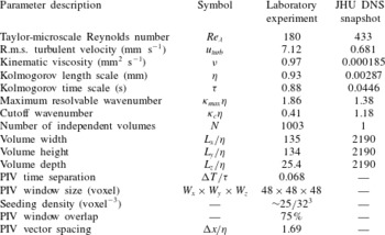
Reference Li, Perlman, Wan, Yang, Meneveau, Burns, Chen, Szalay and Eyink2008). Relevant parameters of both datasets are described in table 1.
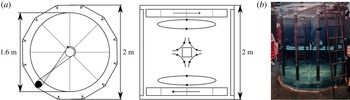
Schematic (a) and photograph (b) of the French washing machine facility.

Relevant parameters for the laboratory experiment and numerical simulation.

3.1. The French washing machine experiment
A brief description of the experimental method is necessary: a full exposition is available in Lawson & Dawson (Reference Lawson and Dawson2014). A hybrid scanning tomographic particle image velocimetry (PIV) system was developed and used to acquire 1003 independent, volumetric, time-series measurements at the centre of a large dodecagonal water tank that was stirred by two counter-rotating impellers in an arrangement commonly known as a ‘French washing machine’. The facility is illustrated in figure 1. The apparatus is 2 m tall and 2 m in diameter. Since the impellers turn slowly, the large scales and therefore the Kolmogorov scales are big and slow, making spatially and temporally resolved measurements possible at reasonably high Reynolds numbers.
At the centre of the tank, the turbulence generated by the impellers and the baffles becomes homogeneous, although there is a secondary, axisymmetric, induced straining flow, which is quite weak in comparison to the turbulence. This large-scale anisotropy persists to the fine scales, where ratios of second-order moments of velocity gradients are consistent with local axisymmetry rather than isotropy (Lawson & Dawson Reference Lawson and Dawson2014).
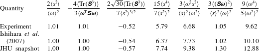
To benchmark the experimental data, a selection of second-, third- and fourth-order moment ratios are provided in table 2. Under homogeneity, the first two ratios should be unity (Betchov Reference Betchov1956), which the experiment satisfies closely. The remaining ratios are the skewness and flatness factors. Comparison to isotropic turbulence data (
 $Re_{{\it\lambda}}=173$
,
 ${\it\kappa}_{\mathit{max}}{\it\eta}=2$
) provided in Ishihara et al. (Reference Ishihara, Kaneda, Yokokawa, Itakura and Uno2007) shows that the experimental data compare quite well, despite the presence of anisotropy. However, the skewness and flatness factors are likely to be slightly underestimated. The ratios for the numerical dataset are also provided.
Ratios of second-, third- and fourth-order moments of velocity gradients for the French washing machine experiment, compared to data from Ishihara et al. (Reference Ishihara, Kaneda, Yokokawa, Itakura and Uno2007) and the snapshot of data taken from the JHU database.

There are 1003 independent, volumetric time-series recordings, which correspond to short movies lasting 600 ms (
 ${\sim}0.68{\it\tau}$
). Each yields a time series of 10 vector fields, separated by a PIV time interval
 ${\rm\Delta}T$
of 60 ms (
 ${\sim}0.068{\it\tau}$
), which determines the temporal resolution. These were post-processed to obtain the pressure field and to reduce measurement noise. Each velocity field was corrected to remove the bias error introduced by scanning (Lawson & Dawson Reference Lawson and Dawson2014). Simulated passive tracers, which advect without slip as
 $\dot{\boldsymbol{X}}(t)=\boldsymbol{u}(\boldsymbol{X}(t),t)$
, are tracked numerically through the volume, starting from grid collocation points
 $\boldsymbol{X}(0)=\boldsymbol{x}_{0}$
. The tracking is performed forwards (up to
 $t=4.5{\rm\Delta}T$
, the tenth vector field in the time series) and backwards in time (to
 $t=-4.5{\rm\Delta}T$
, the first vector field) using a predictor–corrector scheme. The Taylor series expansion of a tracer’s displacement is given as
 $$\begin{eqnarray}{\bf\delta}(\boldsymbol{x}_{0},t)=\boldsymbol{X}(t)-\boldsymbol{X}(0)=\boldsymbol{u}(\boldsymbol{x}_{0},0)t+\left.\frac{\text{D}\boldsymbol{u}}{\text{D}t}\right|_{\boldsymbol{x}_{0},0}\frac{t^{2}}{2}+O(t^{3}).\end{eqnarray}$$
Extracting the odd and even terms of this series and neglecting viscous forces in the material acceleration (as their effect is negligible in comparison to measurement noise), one obtains
 $$\begin{eqnarray}\left.\begin{array}{@{}c@{}}{\bf\delta}^{o}(\boldsymbol{x}_{0},t)={\displaystyle \frac{{\it\delta}(\boldsymbol{x}_{0},t)-{\it\delta}(\boldsymbol{x}_{0},-t)}{2}}=\boldsymbol{u}(\boldsymbol{x}_{0},0)t+O(t^{3}),\\ {\bf\delta}^{e}(\boldsymbol{x}_{0},t)={\displaystyle \frac{{\it\delta}(\boldsymbol{x}_{0},t)+{\it\delta}(\boldsymbol{x}_{0},-t)}{2}}=-\boldsymbol{{\rm\nabla}}p(\boldsymbol{x}_{0},0){\displaystyle \frac{t^{2}}{2}}+O(t^{4}).\end{array}\right\}\end{eqnarray}$$
A set of velocity
 $\boldsymbol{u}(\boldsymbol{x},0)$
and pressure
 $p(\boldsymbol{x},0)$
fields is then determined by applying a least-squares fit of this truncated expression to the Lagrangian time-series data. This process helps to reduce noise in both the velocity and pressure fields, since the acceleration field is expressed as a scalar potential. Tracking tracers requires interpolation: piecewise cubic polynomial interpolation is employed to interpolate in time, and linear interpolation is used to interpolate in space. The grid collocation points
 $\boldsymbol{x}_{0}$
are spaced
 ${\sim}0.85{\it\eta}$
apart, which is twice the PIV resolution, so this process actually upsamples the velocity field in space (making subsequent spatial interpolation more accurate), as well as providing access to the pressure field.
Velocity gradients are calculated using the scheme described by Tokgoz et al. (Reference Tokgoz, Elsinga, Delfos and Westerweel2012): this numerical scheme has a spatial filtering effect, which helps to remove high-wavenumber artefacts introduced by the upsampling process. The pressure gradient field
 $\boldsymbol{{\rm\nabla}}p$
is similarly differentiated to yield experimental measurements of the pressure Hessian. This is certainly a difficult quantity to measure, and one may be concerned about noise and spatial resolution. However, all statistics of the pressure Hessian reported presently have been checked against the numerical dataset: there is good agreement. It is hard to quantify the error in the pressure Hessian measurement, but these checks against the numerical dataset show that the conclusions are unaffected by any such error.
The post-processing routine helps to reduce noise: the r.m.s. dilatation
 $(\langle (\boldsymbol{{\rm\nabla}}\boldsymbol{\cdot }\boldsymbol{u})^{2}\rangle )^{1/2}$
is reduced from 0.089 to
 $0.036~\text{s}^{-1}$
, and the mean of the divergence parameter
 ${\it\xi}$
(3.3),
 $$\begin{eqnarray}{\it\xi}=\frac{(\partial u_{i}/\partial x_{i})^{2}}{(\partial u_{1}/\partial x_{1})^{2}+(\partial u_{2}/\partial x_{2})^{2}+(\partial u_{3}/\partial x_{3})^{2}},\end{eqnarray}$$
is reduced from 0.156 to 0.031. This compares favourably to other experimental turbulence datasets (Mullin & Dahm Reference Mullin and Dahm2006; Ganapathisubramani et al.
Reference Ganapathisubramani, Lakshminarasimhan and Clemens2008), where values of
 $\langle {\it\xi}\rangle$
of 0.12 and 0.18, respectively, are reported.
Table 3 lists the dissipation rate
 $\langle {\it\epsilon}\rangle$
estimated from fits to second- and third-order structure functions and that calculated directly using the relation
 $\langle {\it\epsilon}\rangle =2{\it\nu}\langle S_{ij}S_{ij}\rangle$
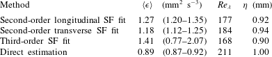
. The 95 % confidence intervals, shown in brackets, were obtained using the bootstrap procedure. Corresponding estimates of the Taylor-microscale Reynolds number and Kolmogorov scale are also shown. The second-order structure function fits have been based on the longitudinal and transverse, isotropic components extracted using the SO(3) symmetry group decomposition (Biferale & Procaccia Reference Biferale and Procaccia2005), taking the Kolmogorov constant to be 2.12 (Sreenivasan Reference Sreenivasan1995). The exact result of Nie & Tanveer (Reference Nie and Tanveer1999) was used to recalculate the dissipation from the third-order structure function: this calculation has been revised from Lawson & Dawson (Reference Lawson and Dawson2014) after an error was discovered in the solid-angle averaging procedure.
Estimates of dissipation rate (brackets show bootstrapped 95 % confidence intervals) made from fits to second- and third-order structure functions and compared to the direct estimate from velocity gradients.

The estimates from the second-order structure function fits approximately agree. The nominal value of the dissipation rate estimated from the third-order structure function is larger, but there is substantial statistical uncertainty in this estimate. The direct estimate is the smallest by some margin: it has been underestimated by 25–37 %, depending on the estimate to which it is compared. Given the statistical uncertainty in the third-order structure function estimate, the authors believe it is more likely that the true figure is closer to the second-order structure function estimates. To within the statistical uncertainty, the indirect estimates are all consistent with a dissipation rate in the range
 $1.20{-}1.25~\text{mm}^{2}~\text{s}^{-3}$
, which gives
 $Re_{{\it\lambda}}\simeq 180$
and the Kolmogorov scales noted in table 1.
The underestimation of the dissipation rate by the direct method raises some questions about spatial resolution: the PIV measurement evidently has some filtering effect at the small scales. A conservative estimate, based on the averaging effect of the interrogation window, puts the non-dimensional cutoff frequency at
 ${\it\kappa}_{c}{\it\eta}=2.8{\it\eta}/W_{x}=0.41$
(Foucaut, Carlier & Stanislas Reference Foucaut, Carlier and Stanislas2004). This is of some concern, since it is the fine-scale quantities that are of interest here. On the other hand, as will become evident in § 4, the influence of this filtering does not appear to be too drastic, because the experimental data remain in good agreement with the numerical simulation. Nonetheless, the authors urge caution in interpreting the experimental data.
3.2. The JHU turbulence database
The numerical dataset from the JHU turbulence database consists of a
 $1024^{3}$
snapshot of the velocity field from a simulation of isotropic, forced turbulence. Following the procedure of Wilczek & Meneveau (Reference Wilczek and Meneveau2014), velocity gradient quantities were computed spectrally after dealiasing with a low-pass filter which cut off wavenumbers above
 ${\it\kappa}_{c}=0.85{\it\kappa}_{\mathit{max}}$
. The pressure Hessian was also computed spectrally, without filtering.
3.3. Comparison to Gaussian fields
Exact results for the Gaussian fields were obtained using some results and procedures outlined in appendices B and C of Wilczek & Meneveau (Reference Wilczek and Meneveau2014). The coefficient functions
 $c_{j}(r)$
are obtained from the appropriate linear combination
 $b_{j}(r)$
, whose exact relation to the longitudinal autocorrelation function
 $f(r)$
and its derivatives can be found in their appendix B. A model spectrum is required to compute
 $f(r)$
. The results presented in this paper use the form outlined in Pope (Reference Pope2000), for
 $Re_{{\it\lambda}}=433$
with
 $C=1.5$
,
 ${\it\beta}=5.2$
,
 $c_{{\it\eta}}=0.40$
and
 $c_{L}=6.33$
. Multiple model spectra were tested, including spectra obtained directly from the JHU database: there are some subtle differences, but these do not affect the main results.
4. Results
4.1. Stochastic estimation
The autocorrelation of
 $Q$
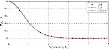
(2.36) is shown in figure 2. This has been calculated for the case of a random, Gaussian velocity field as well as the experimental and numerical datasets. The experimental and numerical datasets are in good agreement when scaled by
 $L_{Q}$
(2.37) and also show agreement with the Gaussian result. The length scale
 $L_{Q}$
is of the order of the Kolmogorov scale, but the ratio
 $L_{Q}/{\it\eta}$
varies slightly between the three cases (see table 4). The spatial resolution of the experiment probably contributes to the larger experimental value of
 $L_{Q}/{\it\eta}$
; Reynolds-number effects may also be at play, since the distribution of radii of intense vortices has a Reynolds-number dependence (Jiménez & Wray Reference Jiménez and Wray1998).
Solid-angle-averaged autocorrelation of
 $Q$
, computed for numerical and DNS datasets and Gaussian random field.

Closure coefficients obtained from various datasets. Superscript prime distinguishes the reversible, enhanced Gaussian closure coefficients from the present, second-order, closure.

It is surprising that there is good agreement between the Gaussian and experimental results, since
 $Q$
is an intermittent quantity, which are generally poorly approximated by Gaussian fields. A distinction will become evident upon comparison of the conditional
 $Q$
field. One might suspect that some degree of cancellation is occurring between
 ${\it\omega}^{2}$
and
 $s^{2}$
to reduce the effect of intermittency upon
 $R_{Q}$
. This observation has precedent: Nelkin (Reference Nelkin1994) notes that some cancellations must occur between
 ${\it\omega}^{2}$
and
 $s^{2}$
to reduce intermittency effects in the pressure spectrum. However, further explanation is beyond the scope of this article.
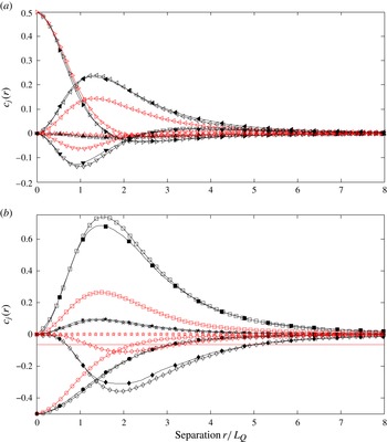
The coefficient functions
 $c_{j}$
are presented in figure 3. These may be interpreted as a set of two-point correlation functions obtained from a multiple-variable linear regression. There is good agreement between the experiment and DNS data, which suggests that the fine-scale structure in both datasets is similar, despite the Reynolds-number difference. Despite the rescaling to match the turbulence data, the Gaussian result is distinct from the experimental and numerical cases: it shows a much more rapid decorrelation of local
 $Q$
field with
 $\unicode[STIX]{x1D63C}$
.
Comparison of coefficient functions
 $c_{j}$
between Gaussian field (unfilled markers, red lines), experiment (unfilled markers, solid lines) and DNS (filled markers, solid lines): (a) terms associated with
 ${\it\tau}_{0}^{-2}$
(
 $c_{1}$
, ▵),
 ${\it\omega}^{2}/2$
(
 $c_{2}$
, ▹),
 $({\bf\omega}\boldsymbol{\cdot }\hat{\boldsymbol{r}})^{2}/2$
(
 $c_{3}$
, ◃) and
 $\hat{\boldsymbol{r}}^{\text{T}}(\unicode[STIX]{x1D64E}\unicode[STIX]{x1D652}-\unicode[STIX]{x1D652}\unicode[STIX]{x1D64E})\hat{\boldsymbol{r}}$
(
 $c_{8}$
, ▿); and (b) terms associated with
 ${\it\tau}_{0}^{-1}\hat{\boldsymbol{r}}^{\text{T}}\unicode[STIX]{x1D64E}\hat{\boldsymbol{r}}$
(
 $c_{4}$
,
 $\star$
),
 $s^{2}$
(
 $c_{5}$
, ○),
 $\hat{\boldsymbol{r}}^{\text{T}}\unicode[STIX]{x1D64E}^{2}\hat{\boldsymbol{r}}$
(
 $c_{6}$
, ▫) and
 $(\hat{\boldsymbol{r}}^{\text{T}}\unicode[STIX]{x1D64E}\hat{\boldsymbol{r}})^{2}$
(
 $c_{7}$
, ♢).

Figure 3(a) shows how vorticity correlates with the local
 $Q$
field. Elevated vorticity at a point correlates with an increase in
 $Q$
in the immediate vicinity (
 $c_{2}$
is positive up to
 ${\sim}1.6L_{Q}$
), with a more pronounced increase in the direction of the vorticity vector, since correlation with
 $({\bf\omega}\boldsymbol{\cdot }\hat{\boldsymbol{r}})^{2}$
(
 $c_{3}$
) persists over a longer distance. Orthogonal to this direction, there is some negative correlation with
 $Q$
, as
 $c_{2}<0$
for
 $r\geqslant 1.6L_{Q}$
, indicating an association with nearby strain-dominated regions. This effectively describes a vortex tube, whose radius is of the order of the Kolmogorov scale. This is consistent with widely reported observations of turbulence ‘worms’. In contrast, the Gaussian result shows that elevated vorticity at a point is associated with more blob-like features. Comparing
 $c_{3}$
shows that the correlation between
 $Q$
and
 $({\bf\omega}\boldsymbol{\cdot }\hat{\boldsymbol{r}})^{2}$
is weaker in the Gaussian case, whilst comparing
 $c_{2}$
shows the correlation between
 $Q$
and
 ${\it\omega}^{2}$
is stronger. In all cases, in comparison to the other terms, the magnitude of
 $c_{1}$
is small, but not vanishing.
Figure 3(b) shows how straining influences the conditional
 $Q$
field, which is embodied by the terms in
 $c_{4}{\it\tau}_{0}^{-1}\hat{\boldsymbol{r}}^{\text{T}}\unicode[STIX]{x1D64E}\hat{\boldsymbol{r}}$
,
 $c_{5}s^{2}$
,
 $c_{6}\hat{\boldsymbol{r}}^{\text{T}}\unicode[STIX]{x1D64E}^{2}\hat{\boldsymbol{r}}$
and
 $c_{7}(\hat{\boldsymbol{r}}^{\text{T}}\unicode[STIX]{x1D64E}\hat{\boldsymbol{r}})^{2}$
. The term in
 $s^{2}$
is sensitive to total strain in an isotropic way, in contrast to the remaining terms. The terms
 $\hat{\boldsymbol{r}}^{\text{T}}\unicode[STIX]{x1D64E}\hat{\boldsymbol{r}}$
and
 $(\hat{\boldsymbol{r}}^{\text{T}}\unicode[STIX]{x1D64E}\hat{\boldsymbol{r}})^{2}$
are sensitive to normal strain, whilst
 $\hat{\boldsymbol{r}}^{\text{T}}\unicode[STIX]{x1D64E}^{2}\hat{\boldsymbol{r}}=(\unicode[STIX]{x1D64E}\hat{\boldsymbol{r}})^{2}$
is sensitive to the total rate of deformation in the
 $\hat{\boldsymbol{r}}$
direction.
Examination of
 $c_{5}$
shows that straining motion is generally associated with negative
 $Q$
in the vicinity of that point (i.e. a strain-dominated region). This strain-dominated region is not spherical, but rather extends outwards towards the direction(s) where the normal strain is large (see
 $c_{7}$
). However, towards the directions of largest deformation (i.e. normal strain and shearing), there is a strong, positive correlation with
 $Q$
, which reaches its peak around
 $1.5L_{Q}$
away from the conditioning point (see
 $c_{6}$
). This indicates the presence of vortices embedded in sheet- or tube-like regions of strain-dominated flow, depending on the configuration of strain eigenvalues.
The term in
 $c_{4}$
is associated with the leading-order effects of irreversibility. In the Gaussian case,
 $c_{4}=0$
, so the closure of the pressure Hessian (2.16) is reversible. However, in the more general case,
 $c_{4}\neq 0$
, and the closure (2.28) is not reversible. This shows that some distinction between compressive and extensional normal strain is felt by the conditional
 $Q$
field. The preference is for regions of positive
 $Q$
(rotation-dominated flow) to appear in the direction of extensional strain rather than compressive strain, although this preference is relatively weak.
The last term (
 $c_{8}$
) is a measure of the correlation between
 $Q$
and the locally induced shearing motion. To see this, note that one can rewrite
 $F_{8}$
as
 ${\bf\omega}\boldsymbol{\cdot }(\hat{\boldsymbol{r}}\times \unicode[STIX]{x1D64E}\hat{\boldsymbol{r}})$
. The vector quantity
 $\hat{\boldsymbol{r}}\times \unicode[STIX]{x1D64E}\hat{\boldsymbol{r}}$
is a measure of the shear experienced by an element pointed in the
 $\hat{\boldsymbol{r}}$
direction and points normal to the plane of shearing. The case where
 ${\bf\omega}$
is aligned with this vector may be described as a shear layer. The
 $F_{8}$
term is therefore strongest in the directions of strongest shear. The associated coefficient function
 $c_{8}(r)$
(figure 3
a) indicates that there is a weak correlation over a nearby region (up to around
 $2L_{Q}$
) with negative (strain-dominated flow) in the direction normal to the shear layer and a positive correlation in the direction along the shear layer.
The closure coefficients
 ${\it\alpha}$
,
 ${\it\beta}$
,
 ${\it\gamma}$
and
 ${\it\delta}$
are presented in table 4. Again, there is good agreement between the experimental and numerical datasets, but the Gaussian closure differs substantially. Additionally,
 ${\it\alpha}^{\prime }$
,
 ${\it\beta}^{\prime }$
and
 ${\it\gamma}^{\prime }$
have been computed according to (2.31), to permit comparison to the EGC. These agree with the values reported by Wilczek & Meneveau (Reference Wilczek and Meneveau2014) to within the margin of error that they report (‘a few per cent’). The neglect of the first-order irreversible term does not affect the calculation of
 ${\it\gamma}^{\prime }$
, so this is the same as
 ${\it\gamma}$
. Further, the values of
 ${\it\alpha}$
and
 ${\it\beta}$
are not too different from
 ${\it\alpha}^{\prime }$
and
 ${\it\beta}^{\prime }$
, so it appears that the implicit reversibility of the EGC does not make much difference to these terms. On the other hand, the experimental and numerical data indicate that the reversible behaviour cannot be quite right, since
 ${\it\delta}\neq 0$
.
When modelling (2.1), introducing the linear (irreversible) term in (2.28) implies that vorticity is damped more strongly than strain in the revised Langevin model (4.1) for (2.5) and (2.7) (Wilczek & Meneveau Reference Wilczek and Meneveau2014):
 $$\begin{eqnarray}\left.\begin{array}{@{}c@{}}\text{d}{\mathcal{S}}^{\star }=\left[-(1+{\it\alpha})\left({\mathcal{S}}^{\star 2}-\frac{1}{3}\text{Tr}({\mathcal{S}}^{\star 2})\unicode[STIX]{x1D644}\right)-(1+{\it\beta})\left({\mathcal{W}}^{\star 2}-\frac{1}{3}\text{Tr}({\mathcal{W}}^{\star 2})\unicode[STIX]{x1D644}\right)\right.\\ -\left.{\it\gamma}({\mathcal{S}}^{\star }{\mathcal{W}}^{\star }-{\mathcal{W}}^{\star }{\mathcal{S}}^{\star })+({\it\zeta}-{\it\delta}){\mathcal{S}}^{\star }\right]\,\text{d}t^{\star }+\text{d}\boldsymbol{F}_{S}^{\star },\\ \text{d}{\bf\omega}^{\star }=[{\mathcal{S}}^{\star }{\bf\omega}^{\star }+{\it\zeta}{\bf\omega}^{\star }]\,\text{d}t^{\star }+\text{d}\boldsymbol{F}_{{\bf\omega}}^{\star }.\end{array}\right\}\end{eqnarray}$$
In (4.1), the superscript
 $\star$
denotes normalisation by
 ${\it\tau}$
;
 $\text{d}\boldsymbol{F}_{S}$
and
 $\text{d}\boldsymbol{F}_{{\bf\omega}}$
represent stochastic forcing. The terms in
 ${\it\zeta}$
model viscous forces as a linear damping. The vorticity equation remains unmodified, but introduction of the linear term in (2.28) changes the damping coefficient for the strain. Based on the derivative skewness
 $S_{3}$
,
 ${\it\zeta}=7S_{3}/6\sqrt{15}\simeq -0.17$
to
 $-0.15$
, which largely cancels with
 ${\it\delta}$
. The effect of this correction upon the model’s performance will be the subject of future work.
4.2. Comparison of conditional structure
Using the procedure outlined in § 2.4, the average
 $Q$
field
 $\langle Q(\boldsymbol{x}+\unicode[STIX]{x1D651}\boldsymbol{r})|{\mathcal{Q}},{\mathcal{R}}\rangle$
is found in a frame of reference aligned with the principal strains, for different conditions on
 $Q$
and
 $R$
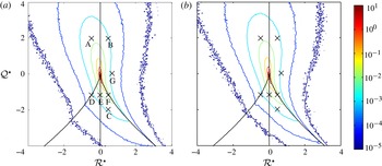
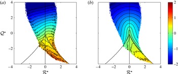
. These are marked in figure 4, which shows the joint p.d.f. of
 $Q$
and
 $R$
, where the axes
 ${\mathcal{R}}^{\star }=R/\langle {\it\omega}^{2}\rangle ^{3/2}$
and
 ${\mathcal{Q}}^{\star }=Q/\langle {\it\omega}^{2}\rangle$
have been normalised with the mean enstrophy. In effect, this is a normalisation by the Kolmogorov time scale, when calculated directly from velocity gradients. The tent-like curve marks the line of zero discriminant
 $D=0$
, known as the Vieillefosse line. The experiment reproduces the characteristic tearing-drop shape of the p.d.f., which reflects the fidelity of the data. The conditional average of
 $\widetilde{A}_{ij}\widetilde{A}_{kl}$
has also been calculated, which is used to calculate the equivalent conditional average using stochastic estimation,
 $\langle \widehat{Q}(\boldsymbol{x}+\unicode[STIX]{x1D651}\boldsymbol{r})|{\mathcal{Q}},{\mathcal{R}}\rangle$
.
Logarithmically spaced contours of joint p.d.f.
 $P({\mathcal{Q}}^{\star },{\mathcal{R}}^{\star })$
, based on (a) numerical and (b) experimental data. Conditions A–G are marked with crosses.

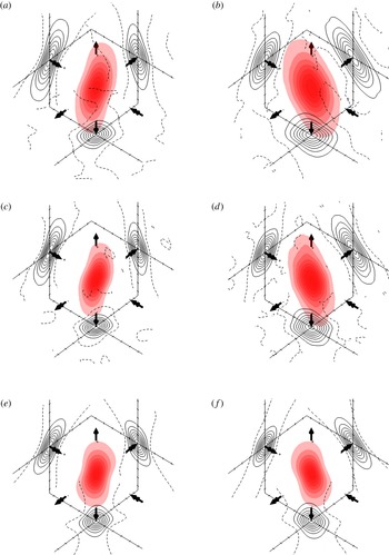
For conditions A–G indicated in figure 4, visualisations have been made of the conditional
 $Q$
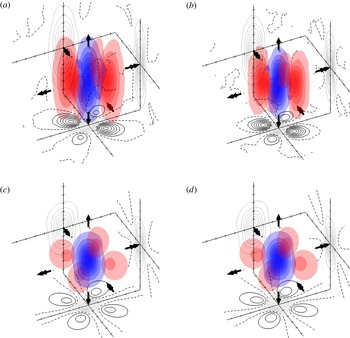
field in figures 5–8. These are somewhat complicated figures, so some description is in order. Large, black arrows indicate the compressive (double-headed arrow pointing inwards), extensional (double-headed arrow outwards) and intermediate (single-headed arrow) straining directions. Translucent isosurfaces of
 $Q^{\prime }>0$
are shown in red, whilst
 $Q^{\prime }<0$
is shown in blue. In the background, contours of
 $Q^{\prime }$
are shown for slices taken through planes
 $\boldsymbol{r}\boldsymbol{\cdot }\boldsymbol{e}_{i}=0$
. Isosurfaces and contours are spaced
 $0.25\langle {\it\omega}^{2}\rangle$
apart, with solid contours corresponding to
 $Q^{\prime }>0$
, dashed contours to
 $Q^{\prime }=0$
and dotted contours to
 $Q^{\prime }<0$
. Finally, to provide a scale, the tick marks in the background are spaced
 $L_{Q}$
apart.
Isosurfaces and contours of conditional
 $Q$
field aligned with strain frame, for conditions A (a,c,e) and B (b,d,f) shown in figure 4: (a,b) correspond to DNS dataset; (c,d) experimental dataset; (e,f) stochastic estimation for experimental dataset.

Condition A (figure 5 a,c,e) corresponds to a fluid in an SF/S topology. Conditional averages for the numerical (figure 5 a) and experimental (figure 5 c) datasets reveal footprints of tube-like rotation-dominated structures, which stochastic estimation also captures (figure 5 e). The axis of the tube is aligned orthogonal to the compressive direction, with some intermediate alignment between the extensional and intermediate straining directions. This is consistent with orientation of the vorticity with respect to the principal axes for this condition. The tubes are surrounded by weakly strain-dominated flow, which mostly falls below the lowest contour level. Conditional average structures from DNS and experiment show good agreement. The stochastic estimation underestimates the length of the rotation-dominated region, as can be identified from the cross-sections, but the phenomenology is the same. This may loosely be described as the footprint left in the pressure field by a collection of stretched vortex tubes. This picture is consistent with that of ‘vortex worms’ and the findings of Nomura & Post (Reference Nomura and Post1998).
Condition B, shown in figure 5(b,d,f), corresponds to fluid in a UF/C topology of the same magnitude as A. There is still an elongated region of rotation-dominated flow, but it is aligned orthogonal to the extensional direction and somewhere between the intermediate and compressive directions. This remains consistent with the conditional mean alignment between vorticity and the strain eigenvectors. The footprint is fatter and distinctly asymmetric in cross-section. The stochastic estimation (figure 5 f) shows a similar picture, but the footprint is shorter and narrower in circumference.
Isosurfaces and contours of conditional
 $Q$
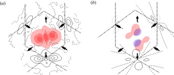
field aligned with strain frame, for condition C shown in figure 4: (a,c) correspond to DNS data and (b,d) to experimental data; (a,b) show true conditional average and (c,d) the stochastic estimation.

Condition C, shown in figure 6, shows a structure representative of that around points in SN/S/S topologies. The footprint left in the
 $Q$
field is substantially different from that surrounding rotation-dominated points. True conditional averages from both datasets (figure 6
a,b) show rotation-dominated regions surrounding a central region of strain-dominated flow. The entire structure is elongated in the
 $\boldsymbol{e}_{2}$
direction. The four rotation-dominated regions are misaligned at approximately
 $45^{\circ }$
to the principal axes. One pair is substantially stronger, aligned with the direction of strongest shearing. This picture is consistent with the (unconditional mean) picture identified by Elsinga & Marusic (Reference Elsinga and Marusic2010b
), who found that, in a reference frame aligned with the principal strains, the predominant flow pattern evidenced in the velocity field is that of a pair of co-rotating vortices aligned in the direction of strongest shear. It is also consistent with the qualitative picture identified in numerous studies (Moisy & Jiménez Reference Moisy and Jiménez2004; Ganapathisubramani et al.
Reference Ganapathisubramani, Lakshminarasimhan and Clemens2008; Bermejo-Moreno et al.
Reference Bermejo-Moreno, Pullin and Horiuti2009) of sheet- or ribbon-like regions of high dissipation near clusters of vortices, with thicknesses of the order of the dissipation scale.
The picture shown by stochastic estimation is similar, but has distinct qualitative differences. As before, rotation-dominated flow sandwiches a central region of strain-dominated flow, which is elongated in the
 $\boldsymbol{e}_{2}$
direction. However, the structure has approximate mirror symmetry about all principal planes
 $\boldsymbol{r}\boldsymbol{\cdot }\boldsymbol{e}_{i}=0$
, i.e. it fails to capture the magnitude of the asymmetry of the rotation-dominated regions (there is asymmetry, but it is quite weak). It is this aspect which results in the model’s failure to correctly capture non-locally induced rotation of the principal strain axes, as will be shown in § 4.4. Furthermore, the entire structure is larger in scale than that identified by the conditional average and the strength of the rotation-dominated regions is underestimated.
As with rotation-dominated structures, the conditional structure identified in figure 6 shows some dependence upon
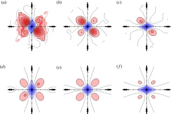
 $R$
. This is evidenced in figure 7, where a projection of the structures corresponding to conditions D–F (figure 4) is shown in the
 $(\boldsymbol{e}_{1},\boldsymbol{e}_{3})$
plane (i.e. viewed from the
 $\boldsymbol{e}_{2}$
direction). The three conditions correspond (approximately) to three limiting configurations of strain eigenvalues: axisymmetric compression (
 ${\it\sigma}_{2}\simeq {\it\sigma}_{3}$
, condition D), plane strain (
 ${\it\sigma}_{2}\simeq 0$
, condition E) and axisymmetric extension (
 ${\it\sigma}_{2}\simeq {\it\sigma}_{1}$
, condition F). The asymmetry of the rotation-dominated regions is most pronounced in condition D, and it is clear that it acts in the wrong sense. As
 $R$
increases, the asymmetry and strength of the rotation-dominated regions decrease and the central, strain-dominated region moves from being more elongated in the compression direction, towards being more elongated in the extensional direction. The stochastic estimation captures the change in shape of the strain-dominated region, but does not correctly capture the changes in the surrounding rotation-dominated regions.
Isosurfaces and contours of conditional
 $Q$
field aligned with strain frame, for conditions D (a,d), E (b,e) and F (c,f) shown in figure 4: (a–c) correspond to true conditional average from experiment and (d–f) their stochastic estimation.

The stochastic estimation deviates substantially from the true conditional average near the right-hand edge of the tearing drop, where neither strain nor rotation may be said to dominate. Figure 8, corresponding to condition G of figure 4, illustrates this point. The average footprint (figure 8
a) resembles that surrounding strain-dominated points, but there is no central strain-dominated region. The stochastic estimation fails to capture this structure (figure 8
b). Examination of the surrounding conditional enstrophy and strain fields (not shown) indicates that there is not, in fact, an absence of rotational and straining motion near the origin. Instead, the strain balances rotation here. This footprint may correspond to an intermediate state between compressed vortex tubes (condition B) and shear layers (condition C). Further conditional averages along the
 $Q=0$
line show a similar structure, even for
 $R<0$
.
Isosurfaces and contours of conditional
 $Q$
field aligned with strain frame, for condition G shown in figure 4: (a) corresponds to true conditional average from experiment and (b) stochastic estimation.

The intention here has not been to catalogue every possible variant of conditional structure. Instead, it has been to broaden the description of the current phenomenology and to identify the most important features. Rotation-dominated points (
 $Q>0$
) tend to be surrounded by long rotation-dominated regions, elongated in the direction of vorticity, although they are not always axisymmetric. Strain-dominated points (
 $D<0$
) are surrounded by clusters of rotation-dominated regions, which are misaligned and show asymmetry with respect to the principal strain axes. Their features tend to be elongated in the intermediate straining direction. There is consistency between the footprint left by turbulent structure in both datasets and with observations of turbulent structure reported elsewhere. Furthermore, stochastic estimation replicates some major qualitative features of this structure, even for relatively extreme conditioning events. Comparison to true conditional averages identifies features that stochastic estimation does not capture.
It is important to note that there is no requirement that conditional averages should map to instantaneous realisations of turbulent structure: conditional averaging reflects the collective footprint left by many structures, grouped under the same condition. However, the consistency of these footprints with previous reports of both instantaneous and averaged flow structures lends some credibility to interpreting these as prototypical structures. On the other hand, this interpretation cannot be strictly true, since the full gamut of turbulent structure cannot just be encoded by single-point measurements of
 $\unicode[STIX]{x1D63C}$
. For example, since large-scale features make a relatively small contribution to
 $\unicode[STIX]{x1D63C}$
, their presence is likely to be averaged out: large-scale clustering of vortex tubes is not evident in these conditional averages, but has been evidenced instantaneously (Leung et al.
Reference Leung, Swaminathan and Davidson2012; Hunt et al.
Reference Hunt, Ishihara, Worth and Kaneda2014). Nonetheless, in the context of single-point statistics of
 $\unicode[STIX]{x1D63C}$
, (2.13) shows that only averages conditional upon
 $\unicode[STIX]{x1D63C}$
matter, so in this case the distinction is not too important.
4.3. Structure and alignments of the pressure Hessian
To understand the role of structure in velocity gradient dynamics, it is useful to take a detour through the alignment statistics of the pressure Hessian with velocity gradients. Alignments between eigenvectors of the pressure Hessian, strain and vorticity have previously been characterised in numerical simulations of isotropic turbulence (Nomura & Post Reference Nomura and Post1998; Kalelkar Reference Kalelkar2006) and compressible turbulence (Suman & Girimaji Reference Suman and Girimaji2013). The discussion here builds upon these results and, as will be shown, provides a structural explanation for the alignment picture.
The argument boils down to how the structures identified in § 4.2 influence the eigenvalues
 $|{\it\pi}_{1}|\geqslant |{\it\pi}_{2}|\geqslant |{\it\pi}_{3}|$
and eigenvectors
 $\boldsymbol{f}_{i}$
of the pressure Hessian
 ${\it\bf\Pi}$
, which it shares with its deviatoric part. The ordering of the eigenvalues
 ${\it\eta}_{i}$
of
 $\unicode[STIX]{x1D643}$
then follows from the ordering of
 ${\it\pi}_{i}$
. To describe the orientation of
 $\boldsymbol{f}_{i}$
with respect to the vorticity and strain eigenvectors, a decomposition in spherical polar coordinates is used, which is illustrated in figure 9(a,b). The polar and azimuthal angles
 $({\it\theta}_{{\it\omega}},{\it\phi}_{{\it\omega}})$
describe the orientation of the vorticity vector with respect to the pressure Hessian eigenvectors. In a similar manner, polar and azimuthal angles
 ${\it\theta}_{i}$
and
 ${\it\phi}_{i}$
describe the orientation of the pressure Hessian eigenvectors
 $\boldsymbol{f}_{i}$
with respect to the principal strain basis.
Definition of polar and azimuthal angles (a)
 ${\it\theta}_{{\it\omega}}$
and
 ${\it\phi}_{{\it\omega}}$
, which describe the orientation of the vorticity with respect to the pressure Hessian eigenvectors, and (b)
 ${\it\theta}_{i}$
and
 ${\it\phi}_{i}$
, which describe the orientation of the pressure Hessian eigenvectors with respect to the strain basis.

Consider the rotation-dominated regions: their footprints are elongated (figure 5) in the direction of the vorticity vector. Consequently, for these regions, one expects the vorticity to tend to align with
 $\boldsymbol{f}_{3}$
(the direction of weakest pressure curvature) and orthogonal to
 $\boldsymbol{f}_{1}$
and
 $\boldsymbol{f}_{2}$
. This is the argument advanced by previous works, which focused on rotation-dominated regions (Ohkitani & Kishiba Reference Ohkitani and Kishiba1995; Nomura & Post Reference Nomura and Post1998). The conditional joint p.d.f. of
 $\cos ({\it\theta}_{{\it\omega}})$
and
 ${\it\phi}_{{\it\omega}}$
for rotation-dominated regions (
 $Q>0$
) is shown in figure 10, calculated from the experimental data. If there were no alignment preference, the joint p.d.f. would take a uniform value of
 $1/4{\rm\pi}$
. Instead, figure 10 shows strong peaks around
 ${\it\phi}_{{\it\omega}}=\pm {\rm\pi}/2$
and
 $\cos ({\it\theta}_{{\it\omega}})=0$
, i.e. the vorticity tends to be parallel to
 $\boldsymbol{f}_{3}$
.
Conditional joint probability density
 $P({\it\theta}_{{\it\omega}},{\it\phi}_{{\it\omega}})$
of polar and azimuthal angles
 ${\it\theta}_{{\it\omega}}$
and
 ${\it\phi}_{{\it\omega}}$
, describing orientation of vorticity with respect to pressure Hessian eigenvectors
 $\boldsymbol{f}_{i}$
, for rotation-dominated regions (
 $Q>0$
) of experimental dataset.

For the strain-dominated regions, structures are elongated in the intermediate strain direction and appear to be broadly symmetric about the
 $\boldsymbol{r}\boldsymbol{\cdot }\boldsymbol{e}_{2}=0$
plane (figure 6). Mirror symmetry in this plane implies
 $\widetilde{H}_{12}=\widetilde{H}_{23}=0$
, which implies that
 $\boldsymbol{e}_{2}$
is an eigenvector of
 $\unicode[STIX]{x1D643}$
. Thus, one expects a tendency for
 $\boldsymbol{e}_{2}$
to align with an eigenvector of
 $\unicode[STIX]{x1D643}$
. Because the structures are elongated in the
 $\boldsymbol{e}_{2}$
direction, it is likely to be the eigenvector associated with least pressure curvature,
 $\boldsymbol{f}_{3}$
. This is evident in the conditional alignment p.d.f. for
 $\boldsymbol{f}_{3}$
with the strain basis (figure 11
c) for strain-dominated regions, which shows a preference for alignment with
 $\boldsymbol{e}_{2}$
(
 $\cos ({\it\theta}_{3})=\pm 1$
).
Conditional joint probability density
 $P({\it\theta}_{i},{\it\phi}_{i})$
of polar and azimuthal angles
 ${\it\theta}_{i}$
and
 ${\it\phi}_{i}$
, describing the orientation of pressure Hessian eigenvectors (a)
 $\boldsymbol{f}_{1}$
, (b)
 $\boldsymbol{f}_{2}$
and (c)
 $\boldsymbol{f}_{3}$
with respect to the strain basis, for strain-dominated regions (
 $D<0$
) of the experimental dataset.

The surrounding rotation-dominated regions are misaligned with the principal axes, towards the direction of strongest shear. Consequently, one expects the directions of strongest pressure curvature,
 $\boldsymbol{f}_{1}$
and
 $\boldsymbol{f}_{2}$
, to point towards the rotation-dominated structures (i.e. towards
 $\boldsymbol{e}_{1}+\boldsymbol{e}_{3}$
or
 $\boldsymbol{e}_{1}-\boldsymbol{e}_{3}$
). As it is associated with the strongest curvature, it is more probable that
 $\boldsymbol{f}_{1}$
is aligned with the strongest pair of rotation-dominated structures, i.e. with the
 $\boldsymbol{e}_{1}-\boldsymbol{e}_{3}$
direction. This is evident in figure 11(a), which shows a strong preference for
 $\boldsymbol{f}_{1}$
to be aligned with
 $\boldsymbol{e}_{1}-\boldsymbol{e}_{3}$
, with a secondary, weaker preference for
 $\boldsymbol{e}_{1}+\boldsymbol{e}_{3}$
. This may occur when
 ${\it\pi}_{1}$
and
 ${\it\pi}_{2}$
are similar in magnitude. Likewise, one expects
 $\boldsymbol{f}_{2}$
to align with the weaker pair, which is evident in figure 11(b). However, alignment statistics for
 $\boldsymbol{f}_{2}$
show the weakest alignment preference, as the joint p.d.f. does not deviate much from uniformity. This may be because
 ${\it\pi}_{2}$
is most likely to switch places with
 ${\it\pi}_{3}$
or
 ${\it\pi}_{1}$
.
One should note that the preceding arguments rely upon interpreting the conditionally averaged structures identified in § 4.2 as prototypes of instantaneous structures, about which the concluding caveat raised concerns. Obviously, instantaneous realisations of structures will deviate from the conditional average, so alignment configurations predicted by the conditional averages are not absolute. The argument therefore rests on how representative the conditional structures are of their instantaneous counterparts, at least with regard to the pressure Hessian, which is most strongly influenced by nearby fluid. The evidence of §§ 4.1 and 4.2 shows that the
 $Q$
field is indeed strongly correlated with
 $\unicode[STIX]{x1D63C}$
(and to a greater extent than the Gaussian case), especially at short distances. Since there is consistency between the alignment statistics of
 $\unicode[STIX]{x1D643}$
and those predicted by the conditional averages, it seems that the distinction does not matter too much in this context.
Figure 12 summarises the alignment configuration of pressure Hessian eigenvectors which predominates at rotation-dominated (figure 12
a) and strain-dominated (figure 12
b) points. For rotation-dominated flow, the vorticity aligns with the direction of weakest pressure curvature
 $\boldsymbol{f}_{3}$
, with any alignment preference with respect to the strain basis dependent upon the degree of vortex stretching or compression. Around strain-dominated points, shear layer structures are largely organised in the extensional–compressive plane and elongated in the intermediate strain direction, resulting in alignment of
 $\boldsymbol{e}_{2}$
and
 $\boldsymbol{f}_{3}$
. The strongest pressure curvature exists in the direction across the strongest pair of vortex cores, so
 $\boldsymbol{f}_{1}$
aligns with
 $(\boldsymbol{e}_{1}-\boldsymbol{e}_{3})$
. The second largest curvature aligns orthogonal to
 $\boldsymbol{f}_{1}$
and
 $\boldsymbol{f}_{2}$
, towards other pairs of cores (if present).
Schematic representation of the typical configuration of vorticity, pressure Hessian and strain eigenvectors in (a) rotation-dominated regions and (b) strain-dominated regions.

4.4. Relation of structure to velocity gradient dynamics
As discussed in § 2.1, the action of non-local effects upon velocity gradient dynamics is directly manifest through the generation of strain (2.5) and only indirectly affects vorticity. Thus, the consequences of structure are presently examined through its effect upon strain production by the deviatoric pressure Hessian
 $\unicode[STIX]{x1D643}$
, which is contrasted to the action of local effects.
The discussion begins with the rotation-dominated regions (
 $Q>0$
), which were shown in § 4.2 to be characterised by elongated vortical structures, where vorticity is aligned with the direction of least pressure curvature
 $\boldsymbol{f}_{3}$
. This configuration persists regardless of the orientation of
 ${\bf\omega}$
with respect to the strain frame. Weak pressure curvature in the
 $\boldsymbol{e}_{{\it\omega}}$
direction implies that
 $H_{{\it\omega}{\it\omega}}\equiv \boldsymbol{e}_{{\it\omega}}^{\text{T}}\unicode[STIX]{x1D643}\boldsymbol{e}_{{\it\omega}}$
scales in proportion to
 $-Q$
. This quantity is shown in figure 13(a), which confirms this scaling. Thus, non-local effects produce extensional strain along the axis of the vortex, since
 $H_{{\it\omega}{\it\omega}}$
is negative. A corollary is that compressive strain is generated in directions orthogonal to the vortex core. If one compares the SF/S and UF/C regions of figure 13(a), it is also apparent that compressed vortices tend to generate less extensional strain along their axis. This is associated with their tendency to be fatter (see figure 5).
Conditional average non-local production of normal strain in
 $\boldsymbol{e}_{{\it\omega}}$
direction by (a) pressure Hessian
 $\langle \boldsymbol{e}_{{\it\omega}}^{\text{T}}\unicode[STIX]{x1D643}\boldsymbol{e}_{{\it\omega}}|{\mathcal{Q}},{\mathcal{R}}\rangle$
and (b) its stochastic estimation
 $\langle \boldsymbol{e}_{{\it\omega}}^{\text{T}}\widehat{\unicode[STIX]{x1D643}}\boldsymbol{e}_{{\it\omega}}|{\mathcal{Q}},{\mathcal{R}}\rangle$
, for experimental dataset. All quantities have been normalised by the appropriate power of
 $\langle {\it\omega}^{2}\rangle$
.

The conditional average of the prediction made by stochastic estimation
 $\widehat{H}_{{\it\omega}{\it\omega}}$
(4.2) differs. This is shown in figure 13(b). It underestimates strain production and fails to reflect differences between stretched and compressed vortices. One can rewrite the expression for
 $\widehat{H}_{{\it\omega}{\it\omega}}$
as
 $$\begin{eqnarray}\widehat{H}_{{\it\omega}{\it\omega}}\equiv \boldsymbol{e}_{{\it\omega}}^{\text{T}}\widehat{\unicode[STIX]{x1D643}}\boldsymbol{e}_{{\it\omega}}={\it\alpha}\left(s_{{\it\omega}}^{2}-\frac{1}{3}s^{2}\right)+\frac{{\it\beta}}{6}{\it\omega}^{2}+\frac{{\it\delta}}{{\it\tau}_{0}}{\it\sigma}_{{\it\omega}},\end{eqnarray}$$
where
 ${\it\sigma}_{{\it\omega}}\equiv \boldsymbol{e}_{{\it\omega}}\unicode[STIX]{x1D64E}\boldsymbol{e}_{{\it\omega}}$
and
 $s_{{\it\omega}}^{2}\equiv \boldsymbol{e}_{{\it\omega}}\unicode[STIX]{x1D64E}^{2}\boldsymbol{e}_{{\it\omega}}$
are measures of the normal strain and the total rate of deformation in the vorticity direction. The term in
 ${\it\beta}$
dominates, which results in strain production scaling with enstrophy (
 ${\it\omega}^{2}$
) and not
 $Q$
. Qualitatively, this is broadly correct: stronger vortices (larger enstrophy) have stronger pressure curvature and therefore more strain generation. Quantitatively, this is incorrect, since strain also plays a role here. The difference in strain production is also manifest in the differences in structure between stochastic estimation and true conditional averages (figure 5). Because stochastic estimation underestimates the spatial coherence of the vortex structures, it predicts shorter cores and consequently less strain production along their axis.
Weighted conditional mean alignment cosines between vorticity and strain eigenvectors
 $\langle ({\bf\omega}\boldsymbol{\cdot }\boldsymbol{e}_{i})^{2}|{\mathcal{Q}},{\mathcal{R}}\rangle /\langle {\it\omega}^{2}|{\mathcal{Q}},{\mathcal{R}}\rangle$
, for experimental data: (a) extensional direction (b) intermediate direction and (c) compressive direction.

When examined on the basis of principal strains, the picture is also consistent with elongated vortices. Consider the production of principal strain by the diagonal entries of
 $\widetilde{\unicode[STIX]{x1D643}}$
(figure 15) in conjunction with the (weighted) conditional mean alignment cosines between the vorticity and principal strains (figure 14). In the SF/S region, the vorticity is largely orthogonal to the compressive direction (figure 14
c), which leads to generation of compressive strain (
 $\widetilde{H}_{33}>0$
, figure 15
e), in proportion to the strength of the vortex. Likewise, in the UF/C region, the vorticity tends to align orthogonal to
 $\boldsymbol{e}_{1}$
(figure 14
a), which similarly leads to the depletion of extensional strain (
 $\widetilde{H}_{11}>0$
, figure 15
a). Whenever vorticity aligns with a principal direction (figure 14), it tends to make the corresponding diagonal entry of
 $\unicode[STIX]{x1D643}$
negative (figure 15), as
 $H_{{\it\omega}{\it\omega}}$
is negative.
Conditional averages (a,c,e) and their stochastic estimation (b,d,f) of on-diagonal components of the pressure Hessian, taken in the strain frame. Components shown are (a,b)
 $\widetilde{H}_{11}$
, (c,d)
 $\widetilde{H}_{22}$
and (e,f)
 $\widetilde{H}_{33}$
. All quantities are non-dimensionalised by the appropriate power of
 $\langle {\it\omega}^{2}\rangle$
.

Conditional averages (a,c,e) and stochastic estimation (b,d,f) of off-diagonal components of the deviatoric pressure Hessian, taken in the strain frame. Components shown are (a,b)
 $\widetilde{H}_{12}$
, (c,d)
 $\widetilde{H}_{13}$
and (e,f)
 $\widetilde{H}_{23}$
. All quantities are non-dimensionalised by the appropriate power of
 $\langle {\it\omega}^{2}\rangle$
.

Conditional averages of the off-diagonal elements of
 $\widetilde{\unicode[STIX]{x1D643}}$
, which act to rotate the strain basis, are shown in figure 16. They show consistency with the predominance of elongated vortices. In the SF/S region, vortex cores (and vorticity) are misaligned with the extensional and intermediate directions and orthogonal to the compressive direction (figure 14), leading to large negative values of
 $\widetilde{H}_{12}$
(figure 16
a) and small values of
 $\widetilde{H}_{13}$
and
 $\widetilde{H}_{23}$
(figure 16
c,e). Likewise, in the UF/C region, vortices tend to align orthogonally to the extensional direction, leading to small values of
 $\widetilde{H}_{12}$
and
 $\widetilde{H}_{13}$
and large negative values of
 $\widetilde{H}_{23}$
.
The stochastic estimation captures the non-local dynamics in the strain basis well, as evidenced by the panels on the right-hand side of figures 15 and 16. In rotation-dominated regions, the
 $\unicode[STIX]{x1D652}^{2}$
term dominates in the expression for
 $\widehat{\unicode[STIX]{x1D643}}$
(2.4). Its least eigenvalue is
 ${\it\beta}{\it\omega}^{2}/6$
and the associated eigenvector is
 $\boldsymbol{e}_{{\it\omega}}$
, whilst the remaining two repeated eigenvalues
 $-{\it\beta}{\it\omega}^{2}/12$
are both positive and their eigenvectors are orthogonal to the vorticity. This is precisely the configuration of eigenvectors outlined in § 4.3. This means it is able to correctly capture the orientation of the vortex cores with respect to the strain basis, which determines the production of principal strain in this region. However, it underestimates the magnitude of this strain production, which leads to the quantitative differences in principal strain production.
Consider the action of local effects upon strain production in rotation-dominated regions. The local production of strain by
 $\unicode[STIX]{x1D647}$
(2.6) is also dominated by the term in
 $\unicode[STIX]{x1D652}^{2}$
. This means that the eigenvectors of
 $\unicode[STIX]{x1D647}$
share a similar configuration to that of
 $\unicode[STIX]{x1D643}$
, but its eigenvalues are of opposite sign and different magnitude. As before, one eigenvector of
 $\unicode[STIX]{x1D647}$
is aligned with
 $\boldsymbol{e}_{{\it\omega}}$
, but its eigenvalue is positive and scales (approximately) as
 ${\it\omega}^{2}/6$
. The remaining two eigenvalues are similar in magnitude and scale as
 $-{\it\omega}^{2}/12$
. In other words, local effects produce compressive strain along the axis of the vortex and extensional strain orthogonal to it. It follows that, for rotation-dominated regions, it is the predominance of vortex tubes that leads non-local effects to counteract local production of strain.
The discussion now turns to the strain-dominated regions. Whilst Nomura & Post (Reference Nomura and Post1998) suggested that there was an absence of distinct structure in strain-dominated regions, the conditional averages reported presently contradict this. One only needs to review their figure 9 to see that, although intense strain-dominated regions are less regular in shape, they are clustered around strong, rotation-dominated regions, which is the important phenomenology reported here.
In strain-dominated regions, alignment statistics and structural features have shown that
 $\boldsymbol{f}_{3}$
, associated with the weakest pressure curvature, tends to align with
 $\boldsymbol{e}_{2}$
. The two remaining eigenvalues of
 ${\it\bf\Pi}$
are negative, associated with the pressure maximum induced in the
 $(\boldsymbol{e}_{1},\boldsymbol{e}_{3})$
plane, so
 ${\it\pi}_{3}$
should be the greatest eigenvalue (
 ${\it\pi}_{3}\geqslant {\it\pi}_{2}$
and
 ${\it\pi}_{3}\geqslant {\it\pi}_{1}$
). Thus
 ${\it\eta}_{3}$
and therefore
 $\widetilde{H}_{22}$
should be large and positive. The conditional averages of
 $\widetilde{H}_{22}$
show that this is indeed the case (figure 15). Furthermore, the conditional averages of
 $\widetilde{H}_{12}$
and
 $\widetilde{H}_{23}$
are small (figure 16), which is consistent with
 $\boldsymbol{e}_{2}$
being aligned with an eigenvector of
 $\unicode[STIX]{x1D643}$
.
The behaviour of
 $\widetilde{H}_{11}$
and
 $\widetilde{H}_{33}$
can be understood by considering the relative strengths of pressure curvature in each principal direction. The component
 $\widetilde{{\it\Pi}}_{22}$
is always the least, but because the shape of the central strain-dominated region depends upon
 $R$
(figure 7), the relative size of
 $\widetilde{{\it\Pi}}_{11}$
and
 $\widetilde{{\it\Pi}}_{33}$
change. Towards the right branch of the Vieillefosse line, this central strain-dominated region is elongated in the extensional direction and thin in the compressive direction, so
 $\widetilde{{\it\Pi}}_{33}$
is larger. As a result,
 $\widetilde{H}_{33}$
is the largest (most negative) diagonal entry. The inverse applies towards the left branch of the Vieillefosse line.
The shear layer structures play a role in turning the strain eigenframe, which is distinct from that of local effects. The vortex structures are misaligned with respect to the compressive–extensional directions (figure 6), which is reflected in the alignment of pressure Hessian eigenvectors with the strain frame (figure 11
a,b). This leads to a misalignment, which implies that
 $\widetilde{H}_{13}$
becomes positive, which is confirmed by figure 16(c). The local rotation by
 $\widetilde{{\it\omega}}_{1}\widetilde{{\it\omega}}_{3}$
is not very active in the strain-dominated regions, because the component in the compressive direction is weak (figure 14
c). This is further confirmed through examination of the stochastic estimation of
 $\widetilde{H}_{13}$
(figure 16
d): the
 ${\it\gamma}$
term tends to average out to zero, whilst the
 ${\it\beta}$
term, which is proportional to
 $\widetilde{{\it\omega}}_{1}\widetilde{{\it\omega}}_{3}$
, is small. The
 ${\it\delta}$
term makes no contribution to the off-diagonals.
Stochastic estimation only partially reproduces the non-local dynamics detailed here. The dominance of the
 $\unicode[STIX]{x1D64E}^{2}$
term in (2.28) implies that the eigenvectors of
 $\widehat{\unicode[STIX]{x1D643}}$
align with those of
 $\unicode[STIX]{x1D64E}$
. This is correct for
 $\boldsymbol{f}_{3}$
: it aligns with
 $\boldsymbol{e}_{2}$
and makes a large positive contribution to
 $\widetilde{H}_{22}$
of the form
 ${\it\alpha}(2{\it\sigma}_{2}^{2}-{\it\sigma}_{1}^{2}-{\it\sigma}_{3}^{2})/3$
. It is not correct for
 $\boldsymbol{f}_{1}$
and
 $\boldsymbol{f}_{2}$
, which are misaligned with
 $\boldsymbol{e}_{i}$
, as they point towards the cores of the rotation-dominated structures. However, it still manages to capture the behaviour of
 $\widetilde{H}_{11}$
and
 $\widetilde{H}_{33}$
, because it correctly reproduces the change in shape of the central, strain-dominated region with
 $R$
(figure 7). The term in
 ${\it\delta}\unicode[STIX]{x1D64E}$
only makes a small contribution to
 $\widehat{\unicode[STIX]{x1D643}}$
(even in strain-dominated regions); for the same reason, it also fails to capture the anomalous alignment statistics.
Stochastic estimation fails to represent the non-local rotation of the strain frame, which results from a misalignment between the eigenvectors of
 $\unicode[STIX]{x1D64E}$
and
 $\unicode[STIX]{x1D643}$
. The two terms in
 $\widehat{\unicode[STIX]{x1D643}}$
capable of representing such a misalignment are those in
 ${\it\beta}$
and
 ${\it\gamma}$
, but these play a relatively small role in strain-dominated regions. This is a consequence of the leading-order approximation of
 $\langle Q^{\prime }|{\mathcal{A}}\rangle$
: extra terms are necessary to capture the misalignment. Wilczek & Meneveau (Reference Wilczek and Meneveau2014) suggested representing such higher-order terms by making the coefficients functions of the invariants of
 ${\mathcal{A}}$
. Through the use of the Cayley–Hamilton theorem, one can show that this represents some, but not all, of the higher-order terms which arise from higher-order truncations of (2.19). Augmenting
 ${\it\alpha}$
or
 ${\it\delta}$
would not alter the eigenvectors of their respective terms and therefore would not address the issue that the eigenvectors of
 $\unicode[STIX]{x1D64E}$
and
 $\unicode[STIX]{x1D643}$
are misaligned. Thus, one would have to substantially modify the
 ${\it\beta}$
or
 ${\it\gamma}$
terms, or introduce extra terms into
 $\widehat{\unicode[STIX]{x1D643}}$
, to capture the alignment configuration.
In strain-dominated regions, the
 $\unicode[STIX]{x1D64E}^{2}$
term of
 $\unicode[STIX]{x1D647}$
dominates the local production of strain. The eigenvectors of
 $\unicode[STIX]{x1D647}$
therefore tend to align with those of
 $\unicode[STIX]{x1D64E}$
, which the above discussion has shown have a systematic alignment with respect those of
 $\unicode[STIX]{x1D643}$
. If one orders the eigenvalues
 ${\it\lambda}_{i}$
and associated eigenvectors
 $\boldsymbol{l}_{i}$
of
 $\unicode[STIX]{x1D647}$
as
 ${\it\lambda}_{1}\geqslant {\it\lambda}_{2}\geqslant {\it\lambda}_{3}$
, one finds that
 $\boldsymbol{l}_{3}$
tends to align with
 $\boldsymbol{e}_{2}$
. Since
 ${\it\lambda}_{3}\leqslant 0$
, local effects produce extensional strain in the
 $\boldsymbol{e}_{2}$
direction (2.10), which therefore acts in opposition to non-local effects (figure 15
c). Owing to continuity, the mean action of
 $\widetilde{L}_{11}$
and
 $\widetilde{L}_{33}$
is to generate compressive strain in the remaining principal directions; similarly, this counters the production of extensional strain by non-local effects in the extensional and compressive directions.
The competition between local and non-local influences upon velocity gradient dynamics is more readily seen when one considers the conditional dynamics of
 $Q$
and
 $R$
. Figure 17 compares the local (a) and non-local (b) contributions to
 $\langle \dot{Q}|{\mathcal{R}},{\mathcal{Q}}\rangle$
and
 $\langle {\dot{R}}|{\mathcal{R}},{\mathcal{Q}}\rangle$
. Whilst the action of the local terms is (by definition) identical for both datasets, there is also excellent agreement across datasets for the non-local contribution (figure 17
b). This is consistent with the notion that the fine-scale structure underlying the observed dynamics is the same in both datasets. Moreover, to the authors’ knowledge, this is the first quantitative comparison of the inviscid, non-local
 $(R,Q)$
plane dynamics between experiment and simulation.
Contribution of (a) local effects (
 $-3R$
and
 $-2/3Q^{2}$
terms) and (b) inviscid non-local effects (
 $\langle \text{Tr}(\unicode[STIX]{x1D63C}\unicode[STIX]{x1D643})|{\mathcal{R}},{\mathcal{Q}}\rangle$
and
 $\langle \text{Tr}(\unicode[STIX]{x1D63C}^{2}\unicode[STIX]{x1D643})|{\mathcal{R}},{\mathcal{Q}}\rangle$
terms) to
 $\langle {\dot{R}}|{\mathcal{R}},{\mathcal{Q}}\rangle$
and
 $\langle \dot{Q}|{\mathcal{R}},{\mathcal{Q}}\rangle$
. Conditional mean vectors from the experimental dataset are shown in red, and from the numerical dataset in blue. All quantities are non-dimensionalised by the appropriate power of
 $\langle {\it\omega}^{2}\rangle$
and both panels use the same scale.

The general tendency is for the non-local terms to oppose local terms, which is well established (Ooi et al.
Reference Ooi, Martin, Soria and Chong1999). A notable exception occurs in the UF/C region for small
 $Q$
, where non-local effects become substantially less active and neither strain nor rotation may be called dominant. This state corresponds to condition G, where there is only weak anisotropy of the flow structure with respect to the principal strain basis (figure 8), which explains why non-local effects become less active here.
It is instructive to express the non-local contributions to
 $\dot{Q}$
and
 ${\dot{R}}$
(2.14) as
 $$\begin{eqnarray}\displaystyle & \dot{Q}^{nl}={\it\eta}_{1}\boldsymbol{f}_{1}^{\text{T}}\unicode[STIX]{x1D64E}\boldsymbol{f}_{1}+{\it\eta}_{2}\boldsymbol{f}_{2}^{\text{T}}\unicode[STIX]{x1D64E}\boldsymbol{f}_{2}+{\it\eta}_{3}\boldsymbol{f}_{3}^{\text{T}}\unicode[STIX]{x1D64E}\boldsymbol{f}_{3}, & \displaystyle\end{eqnarray}$$
 $$\begin{eqnarray}\displaystyle & {\dot{R}}^{nl}={\it\eta}_{1}\boldsymbol{f}_{1}^{\text{T}}\unicode[STIX]{x1D64E}^{2}\boldsymbol{f}_{1}+{\it\eta}_{2}\boldsymbol{f}_{2}^{\text{T}}\unicode[STIX]{x1D64E}^{2}\boldsymbol{f}_{2}+{\it\eta}_{3}\boldsymbol{f}_{3}^{\text{T}}\unicode[STIX]{x1D64E}^{2}\boldsymbol{f}_{3}+{\displaystyle \frac{{\it\omega}^{2}}{4}}H_{{\it\omega}{\it\omega}}, & \displaystyle\end{eqnarray}$$
 $-3R$
and
 $2Q^{2}/3$
to
 $\dot{Q}$
and
 ${\dot{R}}$
, respectively (2.14).
Non-local effects influence
 $Q$
by increasing or decreasing total strain
 $s^{2}$
(4.3). In rotation-dominated regions, because
 ${\it\eta}_{3}$
is negative and the remaining eigenvalues are positive and of similar magnitude, the sign of
 $\dot{Q}^{nl}$
depends upon the normal strain in each eigendirection
 $\boldsymbol{f}_{i}^{\text{T}}\unicode[STIX]{x1D64E}\boldsymbol{f}_{i}$
. Because
 $\boldsymbol{f}_{3}$
aligns with vorticity, enstrophy production determines the sign of the
 ${\it\eta}_{3}$
term, since
 $\boldsymbol{f}_{3}\unicode[STIX]{x1D64E}\boldsymbol{f}_{3}\simeq \boldsymbol{e}_{{\it\omega}}^{\text{T}}Se_{{\it\omega}}$
. For stretched (respectively, compressed) vortices, the term in
 ${\it\eta}_{3}$
is negative (positive), whilst continuity implies that the sum of the remaining terms should also be negative (positive). Vortex stretching prevails when
 $R<0$
, whilst compression prevails when
 $R>0$
, so the effect counteracts the local term. Because enstrophy production is the most significant contribution to
 $R$
, the term in
 ${\it\omega}^{2}$
dominates its evolution (4.4). Since the vortices are elongated,
 $H_{{\it\omega}{\it\omega}}$
is negative, so the dominant contribution to
 ${\dot{R}}^{nl}$
is negative, which is also in opposition to local effects.
In strain-dominated regions, because
 $\boldsymbol{f}_{1}$
and
 $\boldsymbol{f}_{2}$
both tend to align at approximately
 $45^{\circ }$
to the principal strains, the normal strain in either direction is weak. Since
 $\boldsymbol{{\it\eta}}_{3}$
is large, positive and its eigenvector is aligned with
 $\boldsymbol{e}_{2}$
,
 $\dot{Q}^{nl}$
is dominated by the
 ${\it\eta}_{3}$
term, whose sign will depend on whether positive or negative
 ${\it\sigma}_{2}$
predominates or (equivalently) the sign of the local self-amplification of strain
 ${\it\sigma}_{1}{\it\sigma}_{2}{\it\sigma}_{3}$
. Consequently, the non-local contribution to the production of total strain opposes local effects, which is reflected in
 $\dot{Q}^{nl}$
. Regarding
 ${\dot{R}}^{nl}$
, the terms in
 $\unicode[STIX]{x1D64E}^{2}$
dominate, but
 $\boldsymbol{f}_{3}^{\text{T}}\unicode[STIX]{x1D64E}^{2}\boldsymbol{f}_{3}$
is the least in magnitude since
 $\boldsymbol{f}_{3}$
aligns with
 $\boldsymbol{e}_{2}$
. Because of the alignment of
 $\boldsymbol{f}_{1}$
and
 $\boldsymbol{f}_{2}$
,
 $\boldsymbol{f}_{1}^{\text{T}}\unicode[STIX]{x1D64E}^{2}\boldsymbol{f}_{1}$
and
 $\boldsymbol{f}_{2}^{\text{T}}\unicode[STIX]{x1D64E}^{2}\boldsymbol{f}_{2}$
are of similar magnitude. Thus, the contributions of the first two terms dominate and tend to be negative, in opposition to local effects.
4.5. Implications for future stochastic models
Having established the reproducibility of the conditional structure and its connection to the inviscid dynamics, the authors suggest that improved models of the pressure Hessian may benefit from capturing the conditional structure more faithfully. This has already led to one small modification of the EGC: the introduction of irreversibility. The impact of this upon the closure will be quantified in future work. Beyond this, another option is to include higher-order terms in (2.19), but this would introduce many additional terms and numerical concerns and little physical insight.
As an alternative, one might consider introducing conditional averaging into the stochastic estimation process. For example, since the radii of the vortex filaments identified in § 4.2 have a dependence on the axial stretching
 ${\it\sigma}_{{\it\omega}}$
(Jiménez & Wray Reference Jiménez and Wray1998), conditioning on this quantity may better represent the differences between compressed and stretched vortices. The differences between the stochastic and direct estimation of conditional structure are more pronounced in strain-dominated regions. In this case, one may be able to avoid the constraints imposed by the isotropic form of
 $\langle Q^{\prime }|{\mathcal{A}}\rangle$
by modelling
 $\langle Q(\boldsymbol{x}+\unicode[STIX]{x1D651}\boldsymbol{r})|\widetilde{{\mathcal{A}}}\rangle$
. However, such approaches must be treated with caution, since one runs the risk of over-fitting the data. In this regard, some additional constraints are required to justify any further sophistication.
5. Conclusion
In this paper, efforts have been made towards the description and modelling of fine-scale turbulent structure and its consequences for velocity gradient dynamics. This has been motivated by the need for a closure of the pressure Hessian term in dynamical models of velocity gradients, which could lead to better turbulence models. Its conclusions are supported by both experimental (
 $Re_{{\it\lambda}}\simeq 180$
) and numerical (
 $Re_{{\it\lambda}}\simeq 433$
) datasets of homogeneous turbulence. The approach has been to examine the footprints left by structure in the
 $Q$
field, conditional upon the state of the velocity gradient tensor, which have been obtained using two complementary techniques. This permits a correspondence to be made between velocity gradient dynamics and kinematic features of the flow.
Towards the modelling aspect of the problem, the isotropic form for the stochastic estimation of
 $\langle Q^{\prime }|{\mathcal{A}}\rangle$
is derived, retaining terms to second order. It consists of eight coefficient functions, seven of which are independent in homogeneous flows, obtained from two-point correlations of
 $Q$
and
 $\unicode[STIX]{x1D63C}$
. The result strongly resembles the enhanced Gaussian closure (Wilczek & Meneveau Reference Wilczek and Meneveau2014), but makes clear the link between structure and the closure coefficients, explicitly prescribes how they should be calculated and incorporates the effect of irreversibility. Coefficient functions computed for both datasets show good agreement and the closure coefficients also agree closely. This contrasts with the result for a random Gaussian velocity field, which is dissimilar and shows a much weaker and more spatially localised correlation between
 $\unicode[STIX]{x1D63C}$
and the surrounding
 $Q$
field. Stochastic estimation indicates that rotation-dominated regions are organised as thin tubes and surrounded by weaker, strain-dominated flow, consistent with the phenomenology described by previous literature. It further indicates that strain-dominated regions are surrounded by clusters of rotation-dominated regions.
A direct comparison is made between true conditional averages of the
 $Q$
field in both datasets and the stochastic estimation. To reduce the dimension of the conditioning, the conditional
 $Q$
field is evaluated in a reference frame aligned with the principal strain basis and conditional averages are projected in the
 $(R,Q)$
phase plane. Upon comparison, it is seen that vortex tubes remain the dominant feature of rotation-dominated regions for the Reynolds numbers studied, with good agreement between datasets. Furthermore, stochastic estimation educes similar structures with the same alignment properties, although it misrepresents their shape and spatial coherence. This confirms that stretched or compressed vortex tubes dominate the non-local dynamics in the SF/S and UF/C regions. In strain-dominated regions, both datasets confirm that sheet- or tube-like regions of strain-dominated flow are surrounded by regions of intense rotation-dominated flow, which are misaligned with the principal strain axes. These resemble the footprint of the predominant shear layer structures identified by Elsinga & Marusic (Reference Elsinga and Marusic2010b
) in unconditional averages. The stochastic estimation captures most of these features, but fails to correctly capture asymmetry in the distribution of these rotation-dominated regions. These observations provide insight for further model development.
Conditional alignment statistics of the vorticity and the pressure Hessian eigenvectors confirm that, in rotation-dominated regions, the vorticity aligns with the direction of weakest pressure curvature, i.e. along vortex cores. For strain-dominated regions, the alignment configuration of pressure Hessian eigenvectors with respect to the strain basis is consistent with the predominance of shear layer structures. Specifically, the direction of least pressure curvature aligns parallel to the intermediate strain direction
 $\boldsymbol{e}_{2}$
, whilst the direction of strongest pressure curvature is aligned with the direction of shear (
 $\boldsymbol{e}_{1}-\boldsymbol{e}_{3}$
).
Non-local effects directly influence velocity gradient dynamics through strain production. The presence of structure, which has a systematic organisation with respect to the strain and vorticity, is shown to explain why non-local strain production counters that induced locally.
For rotation-dominated regions, owing to the predominance of vortex tubes,
 $\unicode[STIX]{x1D643}$
has two positive eigenvalues and one negative eigenvalue, whose eigenvector points along the axis of the tube. Because of their spatial coherence, the vorticity is aligned with the tube. When tubes point along a given direction, they promote the generation of extensional strain in that direction and compressive strain in directions orthogonal to its axis. Combined with conditional alignment statistics of the vorticity, this explains the qualitative behaviour of strain production and frame rotation by non-local effects. The production of strain by local effects shares this configuration of eigenvectors, but has a different set of eigenvalues, which are of opposite sign: as a consequence, they act in opposition to non-local effects.
The predominant shear layer structures of strain-dominated regions have a geometry which implies that non-local effects favour the production of compressive (negative) intermediate strain. This configuration promotes either the growth or depletion of total strain
 $s^{2}$
, depending on the sign of the intermediate strain eigenvalue, and therefore is in opposition to the dominant local contribution to strain production. This leads the configuration to oppose the self-amplification of strain. These two predominant flow patterns therefore represent a substantial simplification of the role of turbulent structure in the dynamics of velocity gradients.
Acknowledgements
This research was funded by the EPSRC under research grant no. EP/I005879/1. The experimental dataset is freely available to the public or research community and can be obtained by contacting the authors.
Appendix A
In this appendix, the relation is derived between the stochastic estimation of the
 ${\it\alpha}$
,
 ${\it\beta}$
and
 ${\it\gamma}$
parameters and those described by Wilczek & Meneveau (Reference Wilczek and Meneveau2014) in their enhanced Gaussian model. They used the following relations for the coefficients, which are distinguished from the present definition with a superscript prime:
 $$\begin{eqnarray}\displaystyle & {\it\alpha}^{\prime }={\displaystyle \frac{\langle \text{Tr}(\unicode[STIX]{x1D652}^{2}\widetilde{\unicode[STIX]{x1D652}^{2}})\rangle \langle \text{Tr}(\unicode[STIX]{x1D64E}^{2}\unicode[STIX]{x1D643})\rangle -\langle \text{Tr}(\unicode[STIX]{x1D64E}^{2}\widetilde{\unicode[STIX]{x1D652}^{2}})\rangle \langle \text{Tr}(\unicode[STIX]{x1D652}^{2}\unicode[STIX]{x1D643})\rangle }{\langle \text{Tr}(\unicode[STIX]{x1D64E}^{2}\widetilde{\unicode[STIX]{x1D64E}^{2}})\rangle \langle \text{Tr}(\unicode[STIX]{x1D652}^{2}\widetilde{\unicode[STIX]{x1D652}^{2}})\rangle -\langle \text{Tr}(\unicode[STIX]{x1D64E}^{2}\widetilde{\unicode[STIX]{x1D652}^{2}})\rangle \langle \text{Tr}(\unicode[STIX]{x1D652}^{2}\widetilde{\unicode[STIX]{x1D64E}^{2}})\rangle }}, & \displaystyle\end{eqnarray}$$
 $$\begin{eqnarray}\displaystyle & {\it\beta}^{\prime }={\displaystyle \frac{\langle \text{Tr}(\unicode[STIX]{x1D64E}^{2}\widetilde{\unicode[STIX]{x1D64E}^{2}})\rangle \langle \text{Tr}(\unicode[STIX]{x1D652}^{2}\unicode[STIX]{x1D643})\rangle -\langle \text{Tr}(\unicode[STIX]{x1D652}^{2}\widetilde{\unicode[STIX]{x1D64E}^{2}})\rangle \langle \text{Tr}(\unicode[STIX]{x1D64E}^{2}\unicode[STIX]{x1D643})\rangle }{\langle \text{Tr}(\unicode[STIX]{x1D64E}^{2}\widetilde{\unicode[STIX]{x1D64E}^{2}})\rangle \langle \text{Tr}(\unicode[STIX]{x1D652}^{2}\widetilde{\unicode[STIX]{x1D652}^{2}})\rangle -\langle \text{Tr}(\unicode[STIX]{x1D64E}^{2}\widetilde{\unicode[STIX]{x1D652}^{2}})\rangle \langle \text{Tr}(\unicode[STIX]{x1D652}^{2}\widetilde{\unicode[STIX]{x1D64E}^{2}})\rangle }}, & \displaystyle\end{eqnarray}$$
 $$\begin{eqnarray}\displaystyle & {\it\gamma}^{\prime }={\displaystyle \frac{\langle \text{Tr}(\unicode[STIX]{x1D64E}\unicode[STIX]{x1D652}\unicode[STIX]{x1D643})\rangle }{\langle \text{Tr}(\unicode[STIX]{x1D64E}\unicode[STIX]{x1D652}(\unicode[STIX]{x1D64E}\unicode[STIX]{x1D652}-\unicode[STIX]{x1D652}\unicode[STIX]{x1D64E}))\rangle }}. & \displaystyle\end{eqnarray}$$
In (A 1) and (A 2), the short-hand
 $\widetilde{\unicode[STIX]{x1D652}^{2}}=\unicode[STIX]{x1D652}^{2}-\unicode[STIX]{x1D644}\,\text{Tr}(\unicode[STIX]{x1D652}^{2})/3$
and
 $\widetilde{\unicode[STIX]{x1D64E}^{2}}=\unicode[STIX]{x1D64E}^{2}-\unicode[STIX]{x1D644}\,\text{Tr}(\unicode[STIX]{x1D64E}^{2})/3$
has been applied. Wilczek & Meneveau (Reference Wilczek and Meneveau2014) note that this procedure relates the parameter estimates for the pressure Hessian to the flatness factors of the strain and vorticity field, although a more physial explanation is lacking. With the four fourth-order invariants
 $I_{j}$
of
 $\unicode[STIX]{x1D63C}$
(2.34) these relations become
 $$\begin{eqnarray}\displaystyle & {\it\alpha}^{\prime }={\displaystyle \frac{6I_{4}\langle \text{Tr}(\unicode[STIX]{x1D64E}^{2}\unicode[STIX]{x1D643})\rangle +12(I_{2}-3I_{3})\langle \text{Tr}(\unicode[STIX]{x1D652}^{2}\unicode[STIX]{x1D643})\rangle }{I_{1}I_{4}-(I_{2}-3I_{3})^{2}}}, & \displaystyle\end{eqnarray}$$
 $$\begin{eqnarray}\displaystyle & {\it\beta}^{\prime }={\displaystyle \frac{12(I_{2}-3I_{3})\langle \text{Tr}(\unicode[STIX]{x1D64E}^{2}\unicode[STIX]{x1D643})\rangle +24I_{1}\langle \text{Tr}(\unicode[STIX]{x1D652}^{2}\unicode[STIX]{x1D643})\rangle }{I_{1}I_{4}-(I_{2}-3I_{3})^{2}}}, & \displaystyle\end{eqnarray}$$
 $$\begin{eqnarray}\displaystyle & {\it\gamma}^{\prime }={\displaystyle \frac{2\langle \text{Tr}((\unicode[STIX]{x1D64E}\unicode[STIX]{x1D652}-\unicode[STIX]{x1D652}\unicode[STIX]{x1D64E})\unicode[STIX]{x1D643})\rangle }{2I_{2}-3I_{3}}}. & \displaystyle\end{eqnarray}$$
The various contractions with
 $\unicode[STIX]{x1D643}$
can be obtained through substitution of (2.4), application of solid-angle averaging and the definitions of
 $\unicode[STIX]{x1D60D}_{j}$
(2.23). After some algebra, the result is
 $$\begin{eqnarray}\displaystyle & \langle \text{Tr}(\unicode[STIX]{x1D64E}^{2}\unicode[STIX]{x1D643})\rangle =\displaystyle \lim _{{\it\epsilon}\rightarrow 0}\int _{{\it\epsilon}}^{\infty }\left(2\overline{\langle F_{5}Q^{\prime }\rangle }-6\overline{\langle F_{6}Q^{\prime }\rangle }\right)\frac{\text{d}r}{r}, & \displaystyle\end{eqnarray}$$
 $$\begin{eqnarray}\displaystyle & \langle \text{Tr}(\unicode[STIX]{x1D652}^{2}\unicode[STIX]{x1D643})\rangle =\displaystyle \lim _{{\it\epsilon}\rightarrow 0}\int _{{\it\epsilon}}^{\infty }\left(\overline{\langle F_{2}Q^{\prime }\rangle }-3\overline{\langle F_{3}Q^{\prime }\rangle }\right)\frac{\text{d}r}{r}, & \displaystyle\end{eqnarray}$$
 $$\begin{eqnarray}\displaystyle & \langle \text{Tr}((\unicode[STIX]{x1D64E}\unicode[STIX]{x1D652}-\unicode[STIX]{x1D652}\unicode[STIX]{x1D64E})\unicode[STIX]{x1D643})\rangle =\displaystyle \lim _{{\it\epsilon}\rightarrow 0}\int _{{\it\epsilon}}^{\infty }-6\overline{\langle F_{8}Q^{\prime }\rangle }\,\frac{\text{d}r}{r}, & \displaystyle\end{eqnarray}$$
 $F_{8}=\hat{\boldsymbol{r}}^{\text{T}}(\unicode[STIX]{x1D64E}\unicode[STIX]{x1D652}-\unicode[STIX]{x1D652}\unicode[STIX]{x1D64E})\hat{\boldsymbol{r}}$
.
The integrals on the right-hand sides of (A 7)–(A 9) can be simplified by noting that
 $$\begin{eqnarray}\lim _{{\it\epsilon}\rightarrow 0}\int _{{\it\epsilon}}^{\infty }\overline{\unicode[STIX]{x1D60D}_{j}Q^{\prime }}\,\frac{\text{d}r}{r}=\overline{\unicode[STIX]{x1D60D}_{j}\unicode[STIX]{x1D60D}_{k}}C_{k},\end{eqnarray}$$
which follows from the definition of
 $C_{j}$
(2.29). One can therefore obtain expressions for the contractions in
 $\unicode[STIX]{x1D643}$
in terms of
 $\langle \overline{\unicode[STIX]{x1D60D}_{j}\unicode[STIX]{x1D60D}_{k}}\rangle$
and
 $C_{j}$
. The solid-angle-averaged moments
 $\langle \overline{\unicode[STIX]{x1D60D}_{j}\unicode[STIX]{x1D60D}_{k}}\rangle$
can be expressed in terms of the second-, third- and fourth-order invariants of
 $\unicode[STIX]{x1D63C}$
. This is a tedious process, so the result was calculated using symbolic algebra software. By combining the various expressions for
 $\langle \overline{\unicode[STIX]{x1D60D}_{j}\unicode[STIX]{x1D60D}_{k}}\rangle$
, (A 10) and (2.29a−d
) with (A 7)–(A 9), one obtains
 $$\begin{eqnarray}\displaystyle & \langle \text{Tr}(\unicode[STIX]{x1D64E}^{2}\unicode[STIX]{x1D643})\rangle =\displaystyle \frac{{\it\alpha}}{6}I_{1}-\frac{{\it\beta}}{12}(I_{2}-3I_{3})+\frac{{\it\delta}}{{\it\tau}_{0}}T_{1}, & \displaystyle\end{eqnarray}$$
 $$\begin{eqnarray}\displaystyle & \langle \text{Tr}(\unicode[STIX]{x1D652}^{2}\unicode[STIX]{x1D643})\rangle =\displaystyle \frac{{\it\beta}}{24}I_{4}-\frac{{\it\alpha}}{12}(I_{2}-3I_{3})+\frac{{\it\delta}}{4{\it\tau}_{0}}T_{2}, & \displaystyle\end{eqnarray}$$
 $$\begin{eqnarray}\displaystyle & \langle \text{Tr}((\unicode[STIX]{x1D64E}\unicode[STIX]{x1D652}-\unicode[STIX]{x1D652}\unicode[STIX]{x1D64E})\unicode[STIX]{x1D643})\rangle =\displaystyle {\textstyle \frac{1}{2}}(2I_{2}-3I_{3}){\it\gamma}. & \displaystyle\end{eqnarray}$$
The terms in
 $\langle {\it\omega}^{2}\rangle$
and
 $\langle s^{2}\rangle$
from
 $\langle \overline{\unicode[STIX]{x1D60D}_{j}\unicode[STIX]{x1D60D}_{k}}\rangle$
conveniently cancel after substitution into (A 7)–(A 9). Upon substitution of (A 11)–(A 13) into (A 1)–(A 3), one finds
 $$\begin{eqnarray}\displaystyle & {\it\alpha}^{\prime }=\displaystyle {\it\alpha}-{\it\delta}\frac{3}{{\it\tau}_{0}}\frac{T_{2}(I_{2}-3I_{3})+2I_{4}T_{1}}{(I_{2}-3I_{3})^{2}-I_{1}I_{4}}, & \displaystyle\end{eqnarray}$$
 $$\begin{eqnarray}\displaystyle & {\it\beta}^{\prime }=\displaystyle {\it\beta}-{\it\delta}\frac{6}{{\it\tau}_{0}}\frac{2T_{1}(I_{2}-3I_{3})+I_{1}T_{1}}{(I_{2}-3I_{3})^{2}-I_{1}I_{4}}, & \displaystyle\end{eqnarray}$$
 $$\begin{eqnarray}\displaystyle & {\it\gamma}^{\prime }={\it\gamma}, & \displaystyle\end{eqnarray}$$