1. Introduction
Recently, unmanned aerial vehicle (UAV) swarms, incorporating hundreds, even thousands of UAVs, have rapidly received much attention in solving multiple tasks in a cooperative manner, such as aerial light shows and cooperative aerial mapping (Coppola et al., Reference Coppola, McGuire, De Wagter and de Croon2020).
Relative navigation is indispensable to provide individual UAVs with reliable and precise navigation information relative to other UAVs for autonomous swarm flight (Xiong et al., Reference Xiong, Xiong, Cheong, Xu, Yu and Dempster2020). Global navigation satellite system (GNSS)-based relative navigation solutions have enabled impressive cooperative missions on UAV swarms in long-range outdoor environments, for example various commercial aerial light shows by Intel and EHang (Chung et al., Reference Chung, Paranjape, Dames, Shen and Kumar2018) and self-organised swarming in confined environments (Vásárhelyi et al., Reference Vásárhelyi, Virágh, Somorjai, Nepusz, Eiben and Vicsek2018). However, these solutions cannot work well with occlusion or multipath scenarios, and cannot work in GNSS-denied environments.
To expand the application scenario of UAV swarms in long-range outdoor environments, a relative navigation method additionally equipped with onboard sensors (e.g. visual sensor, range sensor, inertial measurement units (IMU)) as an alternative approach has also been widely studied (Chung et al., Reference Chung, Paranjape, Dames, Shen and Kumar2018). With this type of multi-sensor-based solution, Kalman filter (KF)- or extended Kalman filter (EKF)-based multi-agent information fusion algorithms, extended from multi-sensor fusion framework on a single agent, are well understood and widely used models for such multi-agent information fusion problems, for example Vision/Range/IMU-based UAV formation flights (Yuan et al., Reference Yuan, Yang, Zhang and Liang2011), visual inertial odometry swarms (Weinstein et al., Reference Weinstein, Cho, Loianno and Kumar2018) and camera/IMU-based collaborative state estimations (Jung et al., Reference Jung, Brommer and Weiss2020). These relative navigation methods enable UAV swarms to operate in denied environments, as they are independent of the need for external sensors. However, KF/EKF-based algorithms may inadvertently lose rich low-level measuring information representing the nodes’ relative states due to the linearisation procedure; these algorithms rely on detailed geometrical models, which results in these algorithms not being able to handle well sensing uncertainties due to unpredictable measurement bias errors or challenging environments.
By contrast, mammals have evolved reliable and precise absolute/relative navigation ability in challenging environments, especially the highly social bats. Bats can accurately fly in narrow and unstructured caves as well as in visually dark environments in a close and large-scale formation manner (with thousands to millions of individuals) (Genzel et al., Reference Genzel, Yovel and Yartsev2018). Decades of research on hippocampal formation in the mammalian brain have revealed various spatially selective neurons underlying the neural basis of absolute navigation, such as head direction cells, place cells and gird cells. Based on the neurodynamics of these neurons regarding navigation, several impressive brain-inspired navigation models have been proposed and used to perform localisation, mapping and navigation for a single robot, displaying potential robust and flexible navigation performance in challenging environments (Guanella et al., Reference Guanella, Kiper and Verschure2007; Milford and Wyeth, Reference Milford and Wyeth2008, Reference Milford and Wyeth2010; Yuan et al., Reference Yuan, Tian, Shim, Tang and Li2015; Yu et al., Reference Yu, Shang, Hu and Milford2019). Therefore, it is necessary to explore brain-inspired solutions to alleviate problems in multi-agent information fusion algorithms.
Recently, social place cells discovered in the hippocampus (Danjo et al., Reference Danjo, Toyoizumi and Fujisawa2018; Omer et al., Reference Omer, Maimon, Las and Ulanovsky2018) and grid cells in the entorhinal cortex (Bellmund et al., Reference Bellmund, Gärdenfors, Moser and Doeller2018; Schafer and Schiller, Reference Schafer and Schiller2018) are believed to be the neural basis underlying relative navigation of conspecifics, which provide new ideas to find brain-inspired solutions to tackle the problems of the KF/EKF-based relative navigation outlined previously. More recently, Noguchi et al. (Reference Noguchi, Iizuka, Taguchi and Yamamoto2019) implemented the initial idea of a social place cell-based spatial representation model of another individual in a 2D small-scale virtual environment by using a superposition neural network. However, how to implement a neural basis of relative navigation on a robotic system working in a 3D large-scale actual environment remains unclear, particularly in the coordination of movement.
Given this context, based on the neurodynamics of social place cells and grid cells and inspiration from the brain navigation framework of a single robot (Yu et al., Reference Yu, Shang, Hu and Milford2019), we propose a new brain-inspired relative navigation model for collective UAVs. Our contributions:
• Firstly, we develop a novel brain-inspired relative navigation model in a large-scale 3D environment based on neurodynamics of a social place cell-grid cell circuit, which is, to the best of our knowledge, the first work to do so.
• We propose a new 3D isotropic Gaussian function-based cube social place cell network (cube-SPCNet) for encoding an inter-UAV ranging measurement.
• We present a new 3D continuous attractor neural network-based cube grid cell network (cube-GCNet) for integrating relative-motion signals and fusing multi-sensor information from multiple agents.
The rest of the paper is structured as follows: Section 2 provides a brief overview of the social place cell- and grid cell-based neural basis underlying relative navigation; Section 3 describes the proposed brain-inspired relative navigation model in detail; Section 4 presents a potential application scenario of the proposed approach on a UAV swarm flight task (Figure 6), followed by the experimental results and discussions. Section 5 presents the results of the study and reveals the insights of future work.
2. Neural mechanism underlying relative navigation
Along with knowing self-location in space, tracking the vectorial distances of nearby neighbours is a crucial skill for social animals, such as bats and rats, when navigating in groups to perform hunting missions, escape a predator, etc.
Decades of research on hippocampal formation in the mammalian brain have revealed various spatially selective neurons underlying the neural basis of self-navigation in absolute-space coordinates (Moser et al., Reference Moser, Moser and McNaughton2017). At the heart of those neurons is the place cell network in the hippocampus (O'Keefe and Dostrovsky, Reference O'Keefe and Dostrovsky1971; Wohlgemuth et al., Reference Wohlgemuth, Chao and Moss2018) and the grid cell network in the entorhinal cortex (Torkel et al., Reference Torkel, Marianne, Sturla, May-Britt and Moser2005; Kim and Maguire, Reference Kim and Maguire2019). Certain place cells become active when an animal is located in a particular place in an environment. Certain grid cells periodically fire when an animal is in a triangular lattice of physical locations.
A widely held view is that grid cell networks integrate self-motion signal (vectorial velocity) to generate updated estimates of distance relative to a starting point, whereas place cell networks are highly sensitive to changes in landmarks and place cells specifying location input to the grid cell network and anchor grids to environmental cues; the pre-defined associations of place cells to grid cells allow correction of accumulated error due to path integration of the grid cell network (Moser et al., Reference Moser, Moser and McNaughton2017), which has continuously inspired impressive implications in robotic self-navigation (Guanella et al., Reference Guanella, Kiper and Verschure2007; Milford and Wyeth, Reference Milford and Wyeth2008; Yuan et al., Reference Yuan, Tian, Shim, Tang and Li2015; Yu et al., Reference Yu, Shang, Hu and Milford2019).
Recently, increasing evidence suggests a role for encoding the locations of other individuals in the place cell–grid cell circuit in rat, bat and human brains. A part of place cells, identified so-called social place cells also fire in response to the vectorial distances of a conspecific (Danjo et al., Reference Danjo, Toyoizumi and Fujisawa2018; Omer et al., Reference Omer, Maimon, Las and Ulanovsky2018) (see Figure 1). Place cells and grid cells can also contribute to mapping continuous social information in physical space, where nearby positions for similar stimuli to the place-grid cell network and greater distances between dissimilar stimuli (Bellmund et al., Reference Bellmund, Gärdenfors, Moser and Doeller2018; Schafer and Schiller, Reference Schafer and Schiller2018).
Hippocampal–entorhinal cells encode the spatial position of conspecifics: (a and b) social place cells in hippocampus of rat and bat brain fire selectively according to the location in space of another individual. (photo adapted from Duvelle and Jeffery, Reference Duvelle and Jeffery2018); (c and d) place and grid cells map continuous social space. (photo adapted from Bellmund et al., Reference Bellmund, Gärdenfors, Moser and Doeller2018)

We combine the self-navigation processing mechanisms in the place cell–grid cell circuit with the new evidence encoding other's location to propose a spatial representation paradigm, the social place cell–grid cell circuit, for the relative navigation model (Section 3). Grid cells integrate relative-motion signals (relative vectorial velocity) to generate recursive estimates of distance relative to a starting relative distance. Social place cells selectively fire in response to measuring 3D vectorial distances relative to nearby neighbours, and signal to grid cells to calibrate accumulated error through pre-learned connections.
3. Brain-inspired relative navigation for collective UAVs
Relative navigation determines positions relative to other UAVs in a specific relative navigation frame. As shown in Figure 2, the relative navigation process typically consists of two phases (Wymeersch et al., Reference Wymeersch, Lien and Win2009; Yuan et al., Reference Yuan, Yang, Zhang and Liang2011). The first phase is the wireless sensor network measurement in a set of internetworked UAVs, with each UAV equipped with an IMU (measuring angular rate and acceleration), a visual sensor (measuring relative yaw and pitch) and an ultra-wide band (UWB) transceiver (real-time measuring of relative distances relative to other UAVs in the network, while concurrently supporting two-way communication). During this phase, each UAV measures its angular rate and acceleration and figures out its real-time velocity using its own IMU; obtains yaw and pitch relative to its neighbours in sight through its visual sensor; and receives real-time readouts of the velocity of its neighbours and distance relative to its neighbours via UWB, while concurrently emitting its velocity result and distance label (used for relative distance measurement by neighbours) via UWB. The second phase is multi-agent information fusion, during which UAVs infer their own positions relative to other UAVs based on the internal state measurements (self and others) and relative direction and distance measurements using a multi-agent information fusion algorithm.
Schematic diagram of brain-inspired relative navigation for collective UAVs: (a) hierarchical brain-inspired relative navigation framework between UAVi and any other UAV in the swarm; (b) relative navigation frame

This paper focuses on brain-inspired relative navigation by replacing the conventional multi-agent information fusion algorithm (e.g. EKF) with its brain-inspired counterpart – neurodynamics of the postulated social place cell–grid cell circuit.
3.1 Principle of brain-inspired relative navigation
Figure 2 shows the framework of the proposed brain-inspired relative navigation model for the UAV swarm, which is concretised according to its biological counterpart – the postulated social place cell–grid cell circuit (Section 2).
A pair of coupled social place cell–grid cell networks is deployed on UAVi to support relative navigation between UAVi and UAVj. To support simultaneous relative navigation between UAVi and more than one UAV (e.g. more than 10 UAVs), hierarchical pairs of such coupled networks can be deployed on UAVi, with each corresponding to relative navigation between UAVi and any other UAV in the swarm. Each pair of the coupled network consists of three core parts: the social place cell network, grid cell network and neural decoding module.
The social place cell network (using a 3D isotropic Gaussian function) receives relative distance (from UWB) and relative angles (relative yaw and pitch derived from visual sensor) between UAVi and UAVj and then converts these measurements into firing rates of all social place cells in the network (Equation (1)), where each social place cell encodes a pre-defined tuple of relative distance, relative yaw and relative pitch (specifying a particular 3D relative position). The firing rate of each social place cell indicates the probability that the current relative state (relative distance, relative yaw and relative pitch) between UAVi and UAVj is the relative state encoded by that social place cell.
Grid cell network receives relative velocity (derived from a pair of IMUi and IMUj) between UAVi and UAVj. Then, it integrates the relative velocity into the firing rates of all grid cells in the network, where each grid cell encodes a pre-defined 3D relative position between UAVi and UAVj. Similarly, the firing rate of each grid cell indicates the probability that the current relative state (3D relative position) between UAVi and UAVj is the relative state encoded by that grid cell. In addition, specific grid cells also receive firing rates from the corresponding social place cells through the pre-learned connection weights between these two networks (Hebbian learning, Equation (7)). Then, the firing rates of all grid cells will quickly evolve to a stable state through the neurodynamic of the grid cell network (Equations (10)–(16)).
The neural decoding module is the sum of all the 3D relative positions encoded by grid cells, weighted by the corresponding stable firing activity of these cells (Equation (17)). The weighted sum is just the decoded 3D relative positions between UAVi and UAVj.
3.2 Social place cell encoding relative position
This section uses 3D isotropic Gaussian function to model the cube social place cell network (cube-SPCNet). As shown in Figure 3, the $I\times J \times K$ social place cells are arranged in a cube; each cell in the cube is responsible for representing a pre-defined relative tuple $(\varphi ,\theta ,r)$
 (relative yaw, relative pitch, relative distance, respectively), specifying a certain vectorial relative position, obtained from the relative distance/relative yaw and pitch measurement; the most active cells also form a bump; the projection values of the centre of gravity of the bump on the three axes denote the relative tuple at the current moment.
3D isotropic Gaussian function-based social place cell network architecture and response; colour represents the firing rate: light colour corresponds to vanishing rate

The bump in the cube-SPCNet will be driven by relative tuple input obtained from the relative distance /relative yaw and pitch measurement to perform encoding of relative position. The cube-SPCNet is given by

where ${\boldsymbol{S}_{\varphi ,\theta ,r}}$ is $I \times J \times K$
 activity matrix of the cube-SPCNet with each element ${s_{i,j,k}}$
 describing the firing rate of the ${(i,j,k)^{th}}$
 social place cell ranging between 0 and 1; ${\hat{\boldsymbol{S}}_{\varphi ,\theta ,r}}$
 is the normalised activity matrix; $({\varphi _i},{\theta _j},{r_k})$
 is the preferred relative tuple of the ${(i,j,k)^{th}}$
 social place cell; $(\varphi ,\theta ,r)$
 is the relative yaw, relative pitch, relative distance measured from the 3D relative distance surveying unit, respectively.
3.3 Grid cell integrating relative-motion velocity
In this section, we use a 3D continuous attractor neural network to model the cube grid cell network (cube-GCNet). As shown in Figure 4, the cube-GCNet contains $L \times M \times N$ grid cells arranged in a cube, where each cell is interconnected with all the other cells through excitatory and inhibitory weights (Equation (11)). Each cell in the cube-GCNet represents a particular 3D relative position vector; the most active cells form a bump; the projection values of the centre of gravity of the bump on the three axes denote the vectorial relative position at the current moment.
3D continuous attractor neural network-based cube grid cell network architecture and response; colour represents the firing rate: light colour corresponds to vanishing rate

The bump in the cube-GCNet will be first driven to shift by relative-velocity input obtained from a pair of UAVs to perform relative-motion integration:

where $\boldsymbol{S}_{x,y,z}$ is $L \times M \times N$
 activity matrix of the cube-GCNet, with each element describing the firing rate of a grid cell ranging between 0 and 1; $\boldsymbol{S}_{x,y,z}^{\boldsymbol{\prime}}$
 is the activity matrix after integration; $\varDelta x$
 ,$\varDelta y$
 ,$\varDelta z$
 are the rounded down integer offsets along x, y, z directions, respectively (Equation (2)); $\beta$
 represents residue component (Equations (4)–(6)):


where ${v_x}$ ,${v_y}$
 ,${v_z}$
 are vectorial relative-velocity inputs between a pair of UAVs; ${k_x}$
 ,${k_y}$
 ,${k_z}$
 are all constants; $|\!{\underline {\, {} \,}} \cdot {\underline {\, {} \,}}\! |$
 denotes a rounding-down function.
3.4 Information fusion on grid cells
As mentioned in Section 2, there exists accumulated error when the grid cell network integrates vectorial relative-velocity inputs between a pair of UAVs, and calibration from the social place cell network should necessarily be signalled to the grid cell network for information fusion.
This procedure can be successively implemented as social place cell injection and information fusion via attractor dynamics of the cube-GCNet.
Calibration information from the social place cell network will first be injected into the grid cell network through the learned associations between social place cells and grid cells.
The association matrix $\boldsymbol{C}$ is set once at the beginning, through Hebbian learning, in one simulated run over the maximum possible relative distance with noise-free grid cell and social place cell activation.

where ${c_{(i,j,k)(l,m,n)}}$ designates association weight between the ${(i,j,k)^{th}}$
 social place cell and the ${(l,m,n)^{th}}$
 grid cell; ${\hat{s}_{i,j,k}}$
 is the normalised firing rate of the ${(i,j,k)^{th}}$
 social place cell; ${\hat{s}_{l,m,n}}$
 is the normalised firing rate of the ${(l,m,n)^{th}}$
 grid cell; $\eta$
 is the Hebbian learning rate.
The calibration information from the social place cell network can be generated as:

where $\Delta \boldsymbol{S}_{x,y,z}^s$ is the $I \times J \times K$
 injection energy matrix into the cube-GCNet with each element $\Delta s_{l,m,n}^s$
 describing the injection energy into the ${(l,m,n)^{th}}$
 grid cell; $\mu$
 is the injection threshold; ${\hat{s}_{i,j,k}}$
 is the normalised firing rate of the ${(i,j,k)^{th}}$
 social place cell. We define grid cell activity matrix after obtaining the injection energy matrix $\boldsymbol{S}^{\boldsymbol{\prime\prime}}_{x,y,z}$
 following:

Attractor dynamics of cube-GCNet, constituting local excitation and dynamic inhibition, will be next used to fuse the two parts of grid cell activity (injection and integration) in Equation (9). The local excitation can be implemented as

where $\Delta \boldsymbol{S}_{x,y,z}^e$ is the excitatory variable matrix; ${w_{x,y,z}}$
 is the excitatory weight matrix and is created by using a 3D Gaussian distribution. The distribution is calculated by

where ${\delta _x}$ , ${\delta _y}$
 , ${\delta _z}$
 are the constants representing the variance of 3D spatial distributions; ${g_x}$
 ,${g_y}$
 , ${g_z}$
 correspond to the distances between cells in x, y, z direction, respectively. These distances can be calculated as

where $(l^{\prime},m^{\prime},n^{\prime})$ ,$(l^{\prime\prime},m^{\prime\prime},n^{\prime\prime})$
 denote the ${(l^{\prime},m^{\prime},n^{\prime})^{th}}$
 ,${(l^{\prime\prime},m^{\prime\prime},n^{\prime\prime})^{th}}$
 grid cell.
We define the grid cell activity matrix after local excitation $\boldsymbol{S}^{\boldsymbol{\prime\prime\prime}}_{x,y,z}$ following

Then, dynamic inhibition will be next implemented as

where $\Delta \boldsymbol{S}_{x,y,z}^i$ is the locally inhibitory variable matrix; $\gamma$
 denotes the level of global inhibition.
We define grid cell activity matrix after dynamic inhibition $\boldsymbol{S}^{\boldsymbol{\prime\prime\prime}}_{x,y,z}$ following

To keep the sum of activation in the grid cell activity matrix at one, grid cell activity matrix in Equation (13), the normalisation procedure should be necessarily implemented as

where ${\hat{\boldsymbol{S}}_{x,y,z}}$ denotes the normalised grid cell activity matrix; $\max []$
 represent the maximum function.
To produce a 3D relative-position vector $\boldsymbol{r}$ , a centre-of-mass decoder will decode the normalised grid cell activity matrix:

where ${\hat{s}_l}$ , ${\hat{s}_m}$
 , ${\hat{s}_n}$
 are the firing rates of the ${l^{th}}$
 , ${m^{th}}$
 , ${n^{th}}$
 grid cell in the x, y and z direction; ${x_l}$
 , ${y_m}$
 , ${z_n}$
 are the preferred coordinate values of the ${l^{th}}$
 , ${m^{th}}$
 , ${n^{th}}$
 grid cell in the x, y and z direction, respectively.
4. Results and discussions
4.1 Experimental setup
We designed and implemented simulation experiments on MATLAB (2018a) for algorithm validation and performance evaluation using a high-fidelity synthetic dataset. In this section, we describe the flight scenario design, synthetic dataset acquisition, model parameter setting, and evaluation criteria and metric.
(1) Flight scenario design
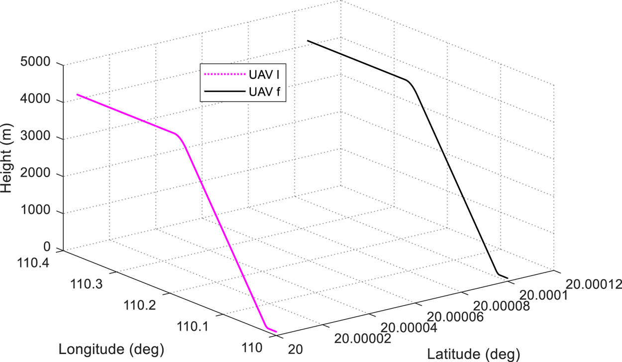
We evaluated our approach on a UAV swarm flight task from Yuan et al. (Reference Yuan, Yang, Zhang and Liang2011), where n UAVs fly in a leader–follower formation flight manner. Since the proposed method is general and scalable to a large number of UAVs, without losing generality, we verified the proposed brain-inspired relative navigation method on one example leader UAV (termed ‘UAVl’) followed by one example follower UAV (termed ‘UAVf’) at a fixed relative distance (Figure 5). The relative flight scenario is structured as follows:
(1) UAVl (UAVf) takes off from 110 ⋅ 0°E, 20 ⋅ 0°N, 100 ⋅ 0 m (110 ⋅ 0002°E, 20 ⋅ 0001°N, 80 ⋅ 0 m) and flies in the east direction at a fixed acceleration and height.
(2) Then, UAVl (UAVf) climbs a slope in the east direction at a fixed acceleration and pitch.
(3) When UAVl (UAVf) rises to 4,350 ⋅ 267 m (4,330 ⋅ 267 m) in height, then UAVl (UAVf) continues to fly in the east direction at a fixed acceleration and height.
(4) Finally, UAVl (UAVf) reaches the terminal position 110 ⋅ 3764°E, 20 ⋅ 0000°N, 4350 ⋅ 267 m (110 ⋅ 3766°E, 20 ⋅ 0001°N, 4330 ⋅ 267 m). The whole flight time lasts for 100 s.
(2) The synthetic dataset is acquired.
Simulation scenario and flight trajectories of two example simulated UAVs

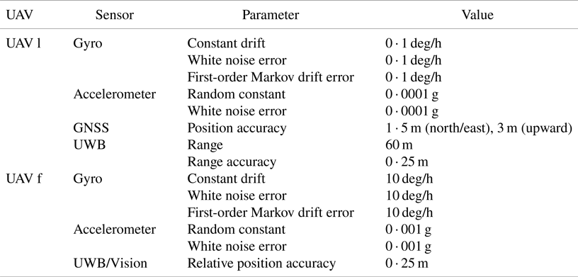
The leader UAV(UAVl) carries a high-precision IMU and GNSS receiver as well as UWB; the follower UAV(UAVf) is equipped with a low-precision IMU and visual sensor as well as UWB; all UAVs in the swarm interconnect with each other within the UWB range. The sensor configuration and the parameters used in the synthetic dataset are listed in Table 1.
Sensor configuration and simulation parameters

Based on these sensor configurations, UAVl and UAVf fly in a leader–follower manner as described in the flight scenario, and output both noised and noise-free sensor date and flight trajectory (real total distance of UAVl or UAVf is 39,918.8 m).
(3) Evaluation criteria and metric
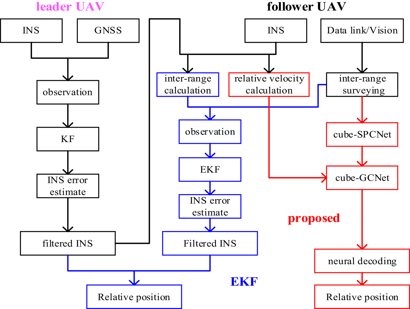
We compare the proposed brain-inspired relative navigation (termed ‘Proposed’) with the widely used EKF-based counterpart (termed ‘EKF’) (Yuan et al., Reference Yuan, Yang, Zhang and Liang2011). The relative navigation frame is an earth-centred earth-fixed frame (ECEF) (Figure 2a). The data flow diagram of these two methods is shown in Figure 6 (Yuan et al., Reference Yuan, Yang, Zhang and Liang2011).
• EKF: UAVl uses KF to fuse its IMU and GNSS data and output the filtered absolute navigation information (filtered INS); UAVf takes the difference between the calculated relative distance (derived from its INS and the INS of UAVl) and the measured relative distance (UWB of UAVf) between itself and UAVl as the observation to correct its INS as its final absolute navigation information by using EKF; the relative position in ECEF between the leader and the UAVf can then be derived from these two filtered INS systems (Figure 6).
• Proposed: The cube-GCNet (grid cell network) of UAVf receives the relative velocity in ECEF (derived from INS of UAVl and INS of UAVf); cube-SPCNet (social place cell network) of UAVf receives the relative distance (from UWB of UAVf) and relative angles in ECEF (relative yaw and pitch from visual sensor of UAVf) between UAVf and UAVl.
(4) Model parameter setting.
Illustration of the comparison of the EKF-based method (black and blue parts) and the proposed method (black and red parts)

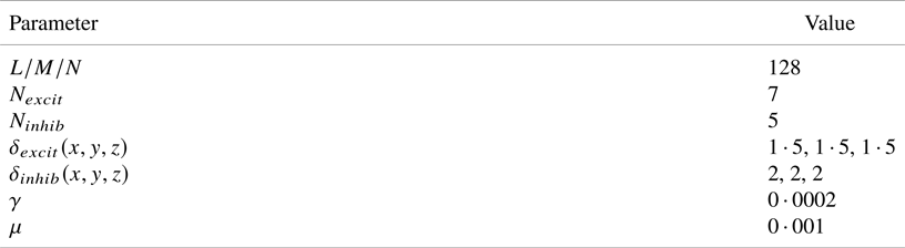
The primary model parameters and their values regarding the proposed method are listed in Table 2 (grid cell network) and Table 3 (social place cell network).
Parameter setting of grid cell network

Parameter setting of social place cell network

The network size (i.e. L/M/N for the grid cell network, I/J/K for the social place cell network) is comprehensively determined according to the relative motion range (line/angular motion) and the desired resolution that each cell can encode. The mathematical formula is

where ${n_c}$ is the network size (L, M, N, I, J, K), ${r_{\max }}$
 (${r_{\min }}$
 ) is the maximum (minimum) value of the relative motion range (line/angular motion), $\lambda$
 is the desired resolution that each cell can encode.
${N_{excit}}$ (${N_{inhib}}$
 ) is the number of nearby cells which each grid cell excites (inhibits) using the excitatory (inhibitory form of the excitatory) weight matrix from Equation (11). ${\delta _{excit}}(x,y,z)$
 (${\delta _{inhib}}(x,y,z)$
 ) controls the magnitude of the excitatory (inhibitory) weight; the larger value indicates a higher excitatory (inhibitory) weight. $\gamma$
 denotes the level of global inhibition; the larger value indicates the stronger inhibition to the firing rate of the grid cell. $\mu$
 is the injection threshold (Equation (8)); the larger value indicates the larger confidence of the relative distance encoded by the social place cell.
${\delta _\varphi }$ (${\delta _\theta }$
 , ${\delta _r}$
 ) is variance constant, which controls the width of the bump of social place cell in the $\varphi$
 ($\theta$
 , $r$
 ) axis; the larger value indicates the larger uncertainty of the relative distance measurement.
4.2 Results and discussions
(1) Results
We first verified the encoding performance of our cube-SPCNet to the input relative distance/relative yaw and pitch measurement between UAV l and UAV f, and the integrating/attractor dynamics-based information fusion performance of our cube-GCNet to relative-motion velocity/calibration (injection energy) from cube-SPCNet.
Figure 7 shows a sequence of snapshots of social place cell activity matrices (a-1 to a-4) and the corresponding grid cell activity matrices (b-1 to b-4) during an information fusion event.
Sequence of snapshots activity in the social place cell matrix (a-1 to a-4) and grid cell matrix (b-1 to b-4) during a certain information fusion event, and the coordinates of the centre of the bumps indicate the current values of relative yaw, relative pitch and relative distance in (a-1 to a-4), relative position after information fusion on grid cells in (a-1 to a-4)

From a-1 to a-4, we find that cube-SPCNet can encode continuous inputs of relative distance/relative yaw and pitch measurements to a sequence of bumps, with each specifying the corresponding vectorial relative positions (as shown on the X, Y, and Z axials, respectively), which suggests that the cube-SPCNet can exactly encode the low-level original measurements to the desired relative navigation information without distorting the original measurements.
From b-1 to b-4, we find that cube-GCNet first integrates relative-motion velocity before receiving injection energy from cube-SPCNet (b-1 to b-2); at b-3, the grid cell activity matrix obtains an injection energy matrix from the social place cell matrix, causing a competing bump (the smaller one) to appear above the existing bump in the grid cell matrix. The attractor dynamics of cube-GCNet fuse the two bumps and produce a new bump centred over the two original bumps. These results suggest the cube-GCNet can perform accurate integration and self-calibration via attractor dynamics.
We also compared our approach with the baseline counterpart – EKF, on the aforementioned UAV swarm flight task to demonstrate the accuracy and robustness of performance.
Figure 8 shows the 3D relative position results of the theoretical one, the EKF-based and the proposed method on the foregoing synthetic dataset, respectively. Figure 9 shows the estimated error of EKF and the proposed method in the X, Y and Z direction in ECEF over time, respectively. Table 4 shows the RMSE of EKF and the proposed method.
Relative position estimate in ECEF: (a) the theoretical relative position in ECEF; (b) the EKF-based relative position in ECEF; (c) the proposed relative position in ECEF

Comparison of relative position estimate error in ECEF

RMSE values of EKF and the proposed method

From these results, we see that:
• The proposed brain-inspired relative navigation method outperforms its conventional counterpart – the EKF-based relative navigation method – in accuracy.
• The proposed method has a stronger ability to self-calibrate cumulative errors than the conventional EKF-based method.
• The proposed method displays a stronger robustness to the jump of the INS inputs.
These results prove a potential application scenario of the proposed brain-inspired relative navigation method for low-cost IMU-based relative navigation enhancement in robustness and accuracy.
(2) Discussions
The conventional KF/EKF-based relative navigation method mainly takes the difference between the relative distance derived from a pair of INS and the relative distance from the relative distance surveying (e.g. UWB) as the observation (Figure 6) to correct INS error. However, this process involves a linearisation procedure, resulting in loss of useful low-level relative distance surveying information. In addition, EKF will have a good effect when the state or observation equation is a closer linear system, and subjects to zero indicate Gaussian noise.
In contrast, the brain-inspired method establishes the calibration of relative distance surveying-based observation to the INS-based relative state through machine learning (Hebbian learning) without a linearisation procedure. In addition, attractor dynamics in the brain-inspired method can well eliminate white noise, constant error, outliers and other unknown types of noise. These two factors enable performance improvement in this brain-inspired method.
For computational efficiency, we conducted experiments with a large-scale social place cell network (128 × 128 × 128) and grid cell network (128 × 128 × 128) using MATLAB (2018a) deployed on a conventional PC platform (ThinkPad T580). The cells-based method is computationally inefficient in terms of computing delay and computing resources compared to a traditional EKF method when using the same hardware platform. With a larger network size, these problems might be more serious.
The principal reason is that the cells-based method uses many neuron nodes and synaptic weights to mimic the neural architecture of the social place cell-grid cell circuit in the brain. Deploying large-scale cell networks on conventional von Neumann hardware will inevitably lead to high computing delay and high occupancy of computing resources.
The cells-based method is specifically designed for neuromorphic hardware, such as Intel's neuromorphic chip – Loihi 2 – which integrates 1 million electronic neuron nodes and 120 million electronic synapses (Mike, Reference Mike2021). Deploying the cells-based method on the neuromorphic hardware by mapping every mathematical neuron node and synapse to the corresponding electronic nodes and synapses will greatly improve the computational efficiency, with lower latency and energy compared to conventional approaches. This we will do in future work.
5. Conclusions
In this paper, we proposed a new brain-inspired relative navigation model for collective UAVs, based on neurodynamics of social place cells and grid cells. The proposed model can achieve better accuracy performance of relative navigation for collective UAVs compared to its conventional counterpart, which loses rich low-level measuring information and sensitive to unpredictable measurement disturbance. It was also, to the best of our knowledge, the first brain-inspired relative navigation model in a large-scale 3D environment.
Future work, including the addition of the online learning rules for achieving association matrix between a social place cell network and grid cell network, coupling of grid cell networks encoding different individuals (Mosheiff and Burak, Reference Mosheiff and Burak2019), the use of graph neural network for swarm optimisation (Khan et al., Reference Khan, Tolstaya, Ribeiro and Kumar2020) and introducing more neural mechanism of spatial cognition and navigation of social animals (Bellmund et al., Reference Bellmund, Gärdenfors, Moser and Doeller2018; Genzel et al., Reference Genzel, Yovel and Yartsev2018), are likely to achieve further performance and capability improvements, and may also yield a new promising paradigm – neuromorphic swarm navigation via conversion from rate-based dynamics to spiking communications (Kreiser et al., Reference Kreiser, Pienroj, Renner and Sandamirskaya2018).
Funding statement
This work was supported by the Basic Science Center Program of the National Natural Science Foundation of China (grant number 62388101); the Application Innovation Program of the Equipment Development Department; the National Natural Science Foundation of China (grant number 61873125); National Defense Basic Research Program (grant number JCKY2020605C009), and the China Scholarship Council (grant number 201906830055).