

INTRODUCTION
The importance of space
Epidemiological models are used by researchers and policy makers alike to explore the processes affecting disease dynamics and to guide the development of disease mitigation strategies. By definition, all pathogens must have some mechanism to ensure their transmission from one host to the next, either through direct contact between infectious and susceptible hosts or via a vector. In both cases, there must be some degree of spatial overlap between hosts, or between hosts and vectors to facilitate transmission. The factors driving the pattern of this overlap, e.g. landscape, climate, habitat, will contribute to the spatial transmission dynamics of the disease.
One common approach to including spatial variation in epidemiological models is to produce large-scale predictive risk maps using geographical information systems (GIS). These typically combine knowledge of host and vector habitat and climate requirements with satellite-imaged data. This has recently been achieved for many diseases, including some tick-borne diseases (TBDs) (e.g. Randolph, Reference Randolph2000; Guerra et al. Reference Guerra, Walker, Jones, Paskewitz, Cortinas, Stancil, Beck, Bobo and Kitron2002; Daniel et al. Reference Daniel, Kolar and Zeman2004; Foley et al. Reference Foley, Queen, Sacks and Foley2005). However, these models are examples of empirical, environmental niche modelling, rather than based on mechanistic processes, because in many cases the causal relationships are poorly understood (e.g. Brownstein et al. Reference Brownstein, Holford and Fish2003). In addition, the host distribution is often ignored, and disease risk predicted on the basis of the vector distribution, rather than of infected vectors (e.g. Guerra et al. Reference Guerra, Walker, Jones, Paskewitz, Cortinas, Stancil, Beck, Bobo and Kitron2002; Brownstein et al. Reference Brownstein, Holford and Fish2003). Most TBDs can infect several different host species, and individual ticks may feed on more than one host species. Therefore, disease transmission depends on the composition, density and spatial distribution of the hosts. Notably, increasing the proportion of hosts with low or no susceptibly will lead to a reduction in disease prevalence – the ‘dilution effect’ (Norman et al. Reference Norman, Bowers, Begon and Hudson1999; Ostfeld and Keesing, Reference Ostfeld and Keesing2000; LoGiudice et al. Reference Brisson, Dykhuizen and Ostfeld2003). Improved risk maps for TBDs therefore need to be compiled by taking into account the complexities of the interactions between hosts, vectors, habitat and climate.
Louping-ill virus
Louping-ill virus (LIV) is a tick-borne flavivirus closely related to the tick-borne encephalitis virus (TBE) found in mainland Europe (Hubalek et al. Reference Hubalek, Pow, Reid and Hussain1995; McGuire et al. Reference McGuire, Holmes, Gao, Reid and Gould1998). It is a widespread disease of domestic livestock in the British Isles, where the primary vector is the sheep tick Ixodes ricinus L. Seroprevalences of up to 90% can be found in untreated sheep (Hudson, Reference Hudson1992). In endemic areas, sheep mortality ranges from 5 to 10%, although it may be as high as 60% in newly introduced individuals (Hudson, Reference Hudson1992). In upland ecosystems, LIV can also infect red grouse Lagopus lagopus scoticus Lath., and has induced 78% mortality in individuals infected by direct inoculation (Reid, Reference Reid and Wild1978). Seroprevalences of up to 80% have been recorded amongst wild red grouse (Laurenson et al. Reference Laurenson, Norman, Gilbert, Reid and Hudson2003).
The ecology of LIV transmission in the Scottish uplands is particularly interesting because it involves complex host-vector-pathogen relationships. Small mammals are relatively scarce on Scottish moorland, and their role in LIV transmission appears to be relatively unimportant (Gilbert et al. Reference Gilbert, Jones, Hudson, Gould and Reid2000). The main tick hosts in this system are sheep, red deer Cervus elaphus L., mountain hares Lepus timidus L. and red grouse. These hosts differ in (a) disease susceptibility, (b) allowing virus transmission and (c) the frequency with which adult reproductive ticks feed upon them. However, it is assumed that sheep can largely be removed from the transmission system by vaccination and/or treatment with acaracides (Laurenson et al. Reference Laurenson, Norman, Reid, Pow, Newborn and Hudson2000), leaving only red grouse as competent for the pathogen. Moreover, red grouse alone cannot support the tick population, since adult ticks are rarely able to feed on them. Although mountain hares do not produce louping-ill viraemia, they do support its transmission via co-feeding ticks (Jones et al. Reference Jones, Gaunt, Hails, Laurenson, Hudson, Reid, Henbest and Gould1997). Red deer do not produce viraemia or allow co-feeding transmission (Jones et al. Reference Jones, Gaunt, Hails, Laurenson, Hudson, Reid, Henbest and Gould1997), but they may still make a significant contribution to the disease dynamics owing to their ability to amplify the tick population (Gilbert et al. Reference Gilbert, Norman, Laurenson, Reid and Hudson2001; Laurenson et al. Reference Laurenson, Norman, Gilbert, Reid and Hudson2003). In contrast to other flaviviruses, including TBE, it appears that LIV is not transmitted transovarially (Hudson et al. Reference Hudson, Gould, Laurenson, Gaunt, Reid, Jones, Norman, MacGuire and Newborn1997).
Attempts to model LIV transmission are still in their infancy. SIR models may not be ideal in all respects, but they are commonly used for modelling disease; whilst the existing LIV models make certain questionable assumptions, they have nevertheless provided good insights. Thus, in the absence of process-based models of the LIV system, we have chosen to develop the SIR approach further. The SIR model of Gilbert et al. (Reference Gilbert, Norman, Laurenson, Reid and Hudson2001) was developed to determine the thresholds at which LIV and the tick population persist in a number of 3-host scenarios, and showed that in the absence of mountain hares, LIV can persist at several combinations of red deer and red grouse densities. However, the virus required increasing grouse density in order to persist as deer densities became increasingly high (c 20 animals km−2 and above), demonstrating a dilution effect through ‘wasted’ tick bites on a non-viraemic host. Laurenson et al. (Reference Laurenson, Norman, Gilbert, Reid and Hudson2003) demonstrated the reduction in LIV at one site following intensive reduction of the mountain hare population. Laurenson et al. (Reference Laurenson, Norman, Gilbert, Reid and Hudson2003) also used the model to support the suggestion that the presence of LIV could contribute to making red grouse harvests economically unviable, although this was challenged by Cope et al. (Reference Cope, Iason and Gordon2004). These influential papers have been used to guide the development of disease management strategies, including culling of hares, on Scottish grouse moors.
In this paper we investigate the limitations of the existing non-spatial SIR model of LIV dynamics by challenging it with new data collected from study areas in Scotland. We then demonstrate the importance of spatial effects, such as host movement, in the system dynamics by extending the original model to a two-patch system, in which one host (red deer) is permitted to move between neighbouring patches.
MATERIALS AND METHODS
Study sites and host density
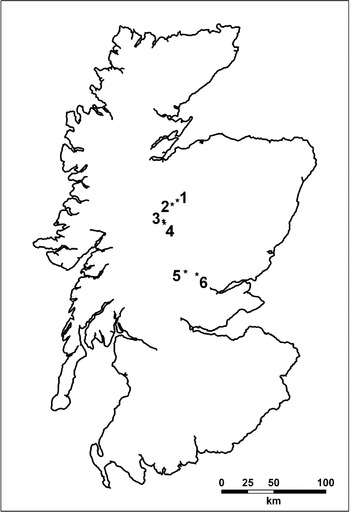
Data were collected from 6 sites in the Scottish Highlands (here numbered 1 to 6, and lying within the region 56°25′–57°5′N, 3°40′–4°15′W; Fig. 1), each comprising 1 km2 of managed grouse moor between 350 and 550 m altitude. Sites were chosen on the basis of having the full complement of hosts (red grouse, sheep, mountain hare and red deer), though varying in their relative abundance, and a heterogeneous moorland habitat maintained through burning. Grouse and hare densities were estimated in summer 2005 from counts using trained pointer dogs. Deer densities were estimated from estate records. Sheep management on all sites was similar and included acaricide and LIV vaccination.
Outline map of Scotland showing the locations of the 6 moorland sites used in this study.

Tick density
An index of tick density was obtained by blanket dragging at 100 points at 100 m intervals on a regular grid within each site (Gray and Lohan, Reference Gray and Lohan1982). The drag comprised a 1 m2 square of pale woollen blanket material, which was pulled across the vegetation for 10 m at each point. Ticks collected were stored in 90% ethanol until later processing. Sites were sampled monthly from May to September in 2004 and 2005, and the exact position of the 10 m×1 m drag was moved each time to avoid re-sampling the same patch. An annual index of tick numbers at each site was obtained by summing the number of ticks counted over all months and drag locations.
Louping-ill virus detection
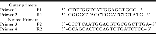
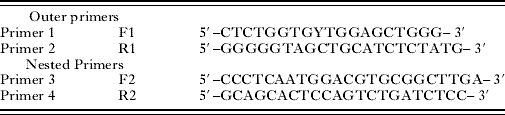
Individual ticks were tested for the presence of LIV RNA using reverse transcriptase polymerase chain reactions (RT-PCR). RNA was extracted from individually homogenized ticks using the RNAgents Total RNA Isolation System (Promega). The presence of LIV RNA was detected using a nested RT-PCR adapted from that used by Gaunt et al. (Reference Gaunt, Jones, Laurenson, Hudson, Reid and Gould1997) and employing different nested primers. Two sets of primers (Table 1) were used to amplify a region of the viral envelope protein RNA. Ten μl of the second PCR product were separated using electrophoresis in ethidium bromide stained agarose gels (1% agarose in 0·5x TAE buffer) and visualized by ultraviolet light transillumination. Samples giving bands of approximately 680 bp were considered to be positive for LIV. A sample of the positive ticks was sequenced to ensure that there had been no cross-contamination from the positive control.
Primer sequences used in the louping-ill nested RT-PCR
(Y denotes a C/T substitution point.)
Where possible, limited samples of hosts were taken from the management ‘beats’ in which the squares were located (a wider area than the 1 km2 itself). These comprised 28 red grouse around site 2 and 40 around site 5 shot in 2004, and 9 mountain hares around site 3 and 14 around site 4 shot in 2005. LIV prevalence in hosts was measured by taking blood samples from culled hosts and conducting haemagglutination-inhibiting antibody tests on the sera.
One patch model
The original model (Gilbert et al. Reference Gilbert, Norman, Laurenson, Reid and Hudson2001; here corrected following Laurenson et al. Reference Laurenson, Norman, Gilbert, Reid and Hudson2003) describes the grouse-hare-deer-tick-LIV system with the following equations:

G, T, H and D are total grouse, tick, hare and deer populations respectively per unit area (here taken to be 1 km2); hare and deer are assumed constant. G i, G s, G z are infected, susceptible and immune grouse populations and T s and T i are susceptible and infected tick populations. s g is a measure of red grouse density dependence, given by the relationship:

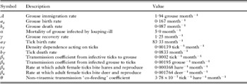
where r is the grouse population growth rate (a g−b g) and K g is the grouse carrying capacity (taken to be the maximum summer count, but see discussion of grouse demography below). Other parameter descriptions and values taken from Gilbert et al. (Reference Gilbert, Norman, Laurenson, Reid and Hudson2001) are given in Table 2. A sensitivity analysis of this model was conducted in order to identify the parameters which could most benefit from improved estimation in future (see Appendix).
Parameter descriptions and values for the one-patch model

This model was implemented in Berkeley Madonna (version 8.3.9) and run for each of the 6 study sites to test its predictions of tick abundance and louping-ill prevalence. Models were run until equilibrium was reached (8–50 years).
Two-patch model
Although the one-patch model was parameterized to represent a relatively large area, the 1 km2 areas studied do not exist in isolation from surrounding moorland which, owing to differences in habitat or management policies, may have a different host composition and/or LIV prevalence. With the exception of allowing constant red grouse immigration, the model acts as though it is a closed system. In reality, there is likely to be a certain degree of host movement between sites, particularly by red deer.
We extended the one-patch model to create a two-patch variant by allowing the movement of red deer (and the ticks they carry) between the two 1 km2 patches, such that:

where v x refers to a variable/parameter of patch X (X=[1,2]) and v y refers to one of patch Y (Y=[2,1], Y≠X), δ is a measure of red deer dispersal (the proportion of deer moving between patches) and β5 is the probability of a nymphs biting a deer. β5 was included in order to allow deer to carry nymphs between the sites and was calculated by the same method (the ratio of nymphs per deer to nymphs per grouse) as the other β terms using the data published in Gilbert et al. (Reference Gilbert, Norman, Laurenson, Reid and Hudson2001). There was a mean of 345 nymphs biting red deer, compared with 9·3 nymphs per grouse, so β5=345β/9·3=37·1β (β=0·0002).
The two-patch model was also implemented in Berkeley Madonna and run to equilibrium as described above for a number of scenarios. (1) We replicated the site C scenario of Gilbert et al. (Reference Gilbert, Norman, Laurenson, Reid and Hudson2001), in which hares were absent (and D=10, K g=30, A=0), adjacent to an otherwise identical site on which hares could be present; the two sites were linked by symmetrical deer movement. (2) Two hypothetical identical sites (having H=3, D=5, K g=24) were linked by asymmetrical deer movement. This could arise in a number of situations, such as sink–source dynamics (Pulliam, Reference Pulliam1988), where deer naturally move from an area of higher net reproductive rate to one of lower net reproductive rate, or where deer movement is driven by differences in culling effort. (3) Our sites 3 and 4 lay on the same sporting estate approximately 1 km apart, but under different management regimes. Although in reality there was a deer-fence separating them, deer may occasionally have been able to move between the sites (e.g. during heavy snow cover or through temporary gaps in the fence). The possibility that such movement could account for the discrepancy between the one-patch model's prediction of no louping-ill persistence at site 3 and the observed prevalence there was therefore examined by coupling these two sites by varying degrees of deer movement between them.
RESULTS
One-patch model
The model tended to underestimate the extent of LIV presence at the study sites. LIV was detected in ticks from all 6 field sites (but did not differ between them: χ2=4·1, d.f.=5, P=0·54), whereas the model predicted its persistence in only 3 of the sites (Table 3a). However, the model apparently overestimated the louping-ill seroprevalence in red grouse. It was estimated as 35% in the area surrounding site 5, which was lower than the predicted prevalence of 62% for the site, and none of 28 red grouse tested around site 2, was seropositive, compared to the model prediction of 85%.
(a) Estimated host densities (mountain hares, red deer and red grouseFootnote a) on 6 Scottish upland grouse moor sites, together with the predicted prevalence of the louping-ill virus from the one-patch model, the observed prevalence determined by detection of viral RNA from samples of red grouse, mountain hares and ticks Ixodes ricinus (adult females and nymphs combined), and the predicted and observed rank order of tick counts

a the summer count of red grouse, made by the local game-keepers, and taken by us to be the only available estimate of grouse carrying capacity for modelling purposes;
‘→0’ indicates that the predicted prevalence tended towards zero; ‘—’ indicates no data were available.
(b) If the grouse carrying capacity K g (here we use the highest values reported by Gilbert et al. Reference Gilbert, Norman, Laurenson, Reid and Hudson2001) and immigration rate A were adjusted for sites 2, 4 and 5 to give approximately their observed grouse densities at equilibrium G*, then the rank order predictions of the number of ticks and LI prevalence in ticks were not altered, but the actual predicted LI prevalence values increased considerably

The model predictions showed a good agreement with the empirical data for the relative number of ticks per site, given the year-to-year variation in the rank order of sites (Table 3a). The only substantial discrepancy in the model rankings was for site 2, where the relative number of ticks was underestimated by the model. The ability of the model to predict LIV prevalence in ticks was much more limited (Table 3a), although interpretation of this finding is more difficult given the high degree of observed annual variation at sites 2 and 3. Moreover, the predicted prevalence was sensitive to the grouse population variables. Table 3a uses the observed grouse density as the carrying capacity, which is unsatisfactory for the sites where louping-ill was predicted to be present (sites 2, 4 and 5), as the predicted equilibrium grouse density was much lower than the observed. Increasing the grouse carrying capacity for these sites, even to double the maximum value reported by Gilbert et al. (Reference Gilbert, Norman, Laurenson, Reid and Hudson2001), did not increase the equilibrium grouse density sufficiently. Increasing the grouse immigration rate did so (Table 3b), but only by applying highly unrealistic values (A=11 equates to 132 immigrant grouse km−2 year−1).
Two-patch model
Scenario 1 – symmetrical deer movement
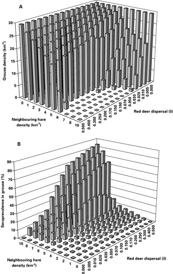
If hares were absent from the neighbouring site or there was no deer movement between sites, the two-patch model behaved as the one-patch model, maintaining a high grouse population and no louping-ill on the focal site. Increasing the hare density on the neighbouring site up to about 5 km−2 had only a very limited effect on the system, unless there was substantial deer movement between sites, in which case the grouse density was reduced by up to about 40% (Fig. 2). However, at greater neighbouring hare densities, even a low level of deer movement between sites led to a rapid decline in the grouse population (Fig. 2A) linked to a sharp rise in louping-ill seroprevalence (Fig. 2B), such that the grouse population could not persist above rates of deer movement between sites ranging from about 3 to 10% per month. Note that apparent fluctuations with increasing deer movement at intermediate hare densities were due to the model's exhibiting extremely long-wavelength damped oscillations under these conditions, which had not quite reached equilibrium even after running the model for 100 years.
The effect on modelled (A) equilibrium red grouse density and (B) louping-ill seroprevalence in red grouse at the focal site of increasing the density of mountain hares on a neighbouring site and the degree of red deer dispersal between the focal site and the neighbouring site. Both sites had grouse carrying capacity of 30 km−2, no grouse immigration and deer density of 10 km−2. Hares were absent from the focal site. Note that the values along the hare density and deer movement axes are categorical rather than continuous, and that the axes' directions are reversed in (B) for clarity.

Doubling the deer density on the two sites to 20 km−2 made very little difference to the qualitative behaviour of the system; it simply increased the threshold neighbouring hare density for grouse persistence from 5 to about 6 km−2 (data not shown). However, the combined effects of high neighbouring hare density and high deer movement on grouse survival could at least be partially overcome by allowing immigration of susceptible grouse (here set at 2 month−1, data not shown).
Scenario 2 – asymmetrical deer movement
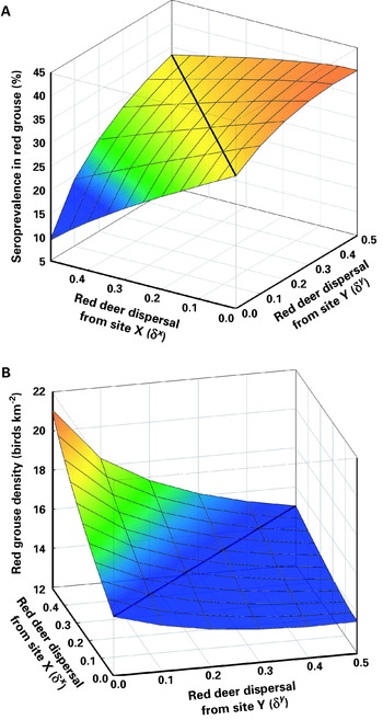
As the disparity between the rates of movement between otherwise identical sites increased, the greater became the difference in louping-ill prevalence in grouse (Fig. 3a), which were always higher on the site where immigration outweighed emigration. A similar response occurred for the prevalence in ticks (not shown). Correspondingly, red grouse density was relatively high only if there was high deer emigration from the site and no compensatory immigration (Fig. 3b). This result seems intuitive, and is in agreement with the predictions of the one-patch model.
The effect of asymmetrical red deer dispersal between 2 otherwise identical sites (H=3, D=5, K g=24) on the predicted (A) louping-ill prevalence in the red grouse population and (B) the equilibrium grouse density at one site X (the second site Y is a mirror image). The heavy lines show where dispersal is symmetrical and the response is constant and equal at the two sites.

Scenario 3 – linking two neighbouring study sites
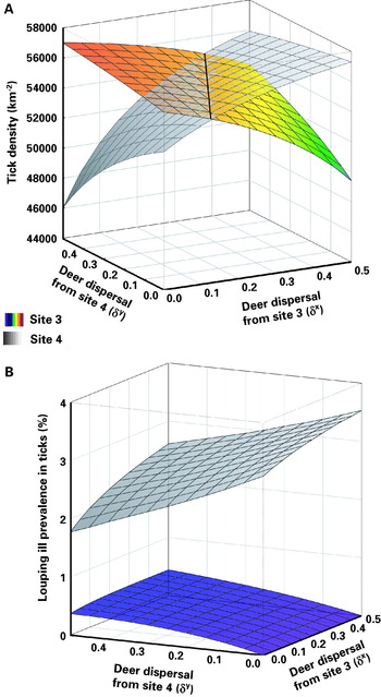
Site 3, which was predicted by the one-patch model to have no louping-ill, actually had a similar proportion of infected nymphs and a far greater proportion of infected hares than site 4 (Table 3a). When modelled red deer movement was symmetrical (δx=δy), increasing the rate of deer movement resulted in a decrease in the number of ticks at site 3 and an increase in tick numbers at site 4 (Fig. 4a). The change in tick numbers was greater at site 4 than at site 3, owing to the fact that the deer moving from site 3 carried more ticks than those moving from site 4. Tick numbers were equal at both sites for δ≈0·26. Also, with increasing red deer dispersal, LIV prevalence in ticks fell slightly at site 4 and rose from zero to low levels at site 3 (Fig. 4b). However, even when deer mixing was at its highest (δx=δy=0·5), the predicted LIV prevalence was still much higher at site 4 than at site 3.
The effect of increasing red deer mixing between 2 sites with different host ratios on (A) the number of ticks and (B) the prevalence of louping-ill virus in ticks, at the two sites. The heavy line in (A) shows where the tick density is equal at the two sites.

Asymmetric red deer movement had a greater effect on site 4 than on site 3 in terms of both tick numbers and disease prevalence (Fig. 4). Tick numbers at each site were maximized when red deer immigration was high and emigration was low. There was a much greater effect of influx of red deer from site 4 (δy) on tick numbers at site 3 when dispersal from site 3 (δx) was high compared to when it was low. Tick density would be equal at the two sites where the planes cross. As empirical data showed that there were more ticks at site 3 than at site 4, the model suggests that the true dispersal parameters should lie to the left of this line. The greater effect of red deer dispersal on tick LIV prevalence at site 4 than at site 3 (Fig. 4b) was due to the fact that the number of mountain hares present has a greater effect on prevalence than the number of red deer does. Therefore, although LIV can be introduced to a site by ticks on roaming red deer, it cannot then reach high levels unless other factors are also acting.
Applying asymmetric red deer dispersal of just 1% from site 4 to site 3 (δy=0·01, δx=0) was enough to maintain the presence of LIV in ticks at site 3. This is equivalent to 1 deer every 4·2 months or just less than 3 deer per year.
DISCUSSION
Importance of spatial effects
The results of the two-patch model demonstrated here indicate how incorporating the effects of spatial variation in SIR models may influence the conclusions drawn. In this case, the inclusion of spatial variation in host abundance and movement of a host between patches allowed the virus to persist where otherwise it would not have, and also resulted in more accurate prediction of the disease vector's abundance. Similar insights have recently been obtained regarding the effect of deer exclosures on Ixodes ricinus densities and TBE prevalence (Pugliese and Rosà, Reference Pugliese and Rosà2008) and for nematode parasites of ungulates (Morgan et al. Reference Morgan, Medley, Torgerson, Shaikenov and Milner-Gulland2007). These findings have significant implications for the development of GIS-based risk maps, and highlight the importance of including host demography and ranging behaviour if such maps are to provide meaningful predictions under various environmental change scenarios.
Implications of effect of host movement on management strategies
These findings can have very important implications for management strategies. The results of the one-patch model suggest that LIV would not persist in a red deer–red grouse system when grouse density falls below 30 km−2 (Gilbert et al. Reference Gilbert, Norman, Laurenson, Reid and Hudson2001). However, our field data showed that not to be the case. Allowing a small proportion of the red deer population to move between a site having moderately high hare density and a site having no hares was enough to allow the LIV to persist at the hare-free site, even at very low deer densities. Laurenson et al. (Reference Laurenson, Norman, Gilbert, Reid and Hudson2003) successfully demonstrated at a single site that LIV prevalence in red grouse could be reduced by the suppression of the mountain hare population where red deer numbers were very low. However, anecdotal evidence suggests that this is not always the case. The two-patch model shows that at a site where red deer are largely absent, even the presence of a small number of deer roaming through the area from a neighbouring site may be enough to maintain a higher than expected level of LIV, which would prevent the culling of hares from having the expected effect on LIV prevalence.
However, it has been argued (e.g. Ruxton, Reference Ruxton1996; Law et al. Reference Law, Murrell and Dieckmann2003) that differential equation models are unsuitable for modelling ecological systems in which spatial structure is important, as they assume free mixing within the population(s) of interest, and that spatially-explicit models would be more appropriate. The louping-ill system incorporates several inherent scales of spatial structure. At the smallest, larval ticks are highly overdispersed owing to their extremely limited dispersal from the single oviposition site. Red grouse are territorial for much of the year (Jenkins et al. Reference Jenkins, Watson and Miller1963), although not so during the summer brood-rearing period (Palmer and Bacon, Reference Palmer and Bacon2001). Hare populations may possibly impose less spatial structure, as hares have been reported as having quite large home ranges (Hewson and Hinge, Reference Hewson and Hinge1990). Sheep and deer, although also ranging widely, may introduce spatial structure by their flocking/herding behaviour. Moreover, these levels of spatial structure are themselves influenced by habitat heterogeneity at a number of scales (e.g. Palmer et al. Reference Palmer, Hester, Elston, Gordon and Hartley2003).
Discrepancies between the one-patch model and empirical data
The one-patch model (Gilbert et al. Reference Gilbert, Norman, Laurenson, Reid and Hudson2001) was shown to be a reasonable predictor of the rankings of tick numbers over a range of sites, although it was less able to predict the LIV prevalence accurately. In part, this may be because the input host densities were inaccurate. Of particular concern are the grouse densities, as, in the absence of any other information, we had to use them to represent the grouse carrying capacity. If they were, indeed, too low, by virtue of the grouse numbers being at the low point of a cyclic fluctuation at a particular site, then that could lead to prediction of louping-ill absence (sites 1, 3 or 6) when actually it should be predicted as present. Moreover, as host densities were provided to us lacking estimates of uncertainty, we cannot say how likely it is that it was the model or the data which caused the discrepancies.
However, adding a second patch to the model could also go some way to explaining the discrepancies between the one-patch model predictions and field data. Although it was possible to inflate the predicted LIV prevalence at a given site through the movement of red deer between adjacent sites, it was not possible to manufacture a scenario where the LIV prevalence, either in ticks or red grouse, actually attained the levels measured at those sites. That may be because the two-patch model remains spatially simplistic; in reality the moorland ecosystem comprises many patches all interacting with their neighbours through the spatial behaviour of all the host species. Perhaps more importantly, however, although the structural simplicity of the differential equation SIR model renders it appropriate to the examination of generic patterns, its inherent assumptions lead to serious shortcomings when it is applied to specific scenarios. We now consider how these problems might be addressed in future modelling developments.
Potential improvements to the SIR model
Temporal dynamics
In differential equation SIR models, the processes occur in continuous time, and it is typically implicitly assumed that the parameters are temporally and spatially constant. Whether this is appropriate for any temperate ecosystem, especially one where host and vector activity show considerable seasonal variation, is cause for some debate. The seasonal dynamics of ticks have been studied extensively (e.g. MacLeod, Reference MacLeod1939; Randolph, Reference Randolph2004 and references therein). Although the precise nature of the seasonality in tick activity may vary with location, it is generally much reduced during winter. The assumption of an unvarying red grouse birth rate is also clearly over-simplistic, as grouse reproduction is highly seasonal. This is potentially very important, as the period of infection of grouse as chicks is actually quite limited. Furthermore, predicted temperature increases will accelerate tick development rates (Randolph, Reference Randolph2004), which may have a substantial impact on the ability of ticks to quest for a host during this crucial period. For this reason, it could be more appropriate to model the system in discrete time and allow variable parameters to reflect the seasonal dynamics of the system.
Tick demography and viral transmission
Infection rates of ticks by different infective hosts are currently assumed to be independent and additive. This probably does not matter much provided that infection rates remain low, but it would do so if they were high. An Ixodid tick can bite only a single host at a given stage of its life-cycle (Randolph, Reference Randolph2004); hence we really need to model the probability that a susceptible tick bites an infective host (of a given species) within a specified time-step and likewise the probability that it bites a non-infective host (Brisson et al. Reference Brisson, Dykhuizen and Ostfeld2008). If it fails to do either within 1 year (according to the assumption made by Gilbert et al. Reference Gilbert, Norman, Laurenson, Reid and Hudson2001), then it dies. This would remove the need for a specific tick death rate parameter, the least well known of tick demographic parameters, to which we have shown the model to be highly sensitive (see Appendix). As considerable assumptions were made in the estimation of the tick demography parameters (Gilbert et al. Reference Gilbert, Norman, Laurenson, Reid and Hudson2001), their refinement should be a matter of priority.
Inaccurate prediction of the percentage of ticks infected at equilibrium could arise because the life-stages of the tick are not distinguished in the model. If considering habitat-specific spatial effects, it could be important to do so, as larvae will be far more over-dispersed than nymphs or adult ticks. Moreover, the time-delays between each stage questing for a host are likely to have important consequences for the system dynamics (Hancock and Godfray, Reference Hancock and Godfray2007). The potential impact of alternative routes of infection on louping-ill dynamics, e.g. if grouse chicks consume infected ticks (Gilbert et al. Reference Gilbert, Jones, Laurenson, Gould, Reid and Hudson2004), is also yet to be explored.
Grouse demography
The imposition of a grouse carrying capacity, to which the model was sensitive (see Appendix), runs contrary to their propensity to exhibit cyclic fluctuations (Moss and Watson, Reference Moss and Watson1991; Hudson et al. Reference Hudson, Newborn and Dobson1992; Cope et al. Reference Cope, Iason and Gordon2004). Even if a carrying capacity truly exists, it cannot be measured in the presence of LIV-induced mortality. Moreover, as no explicit distinction is made between adults and chicks, the density-dependent constraint on grouse fecundity operates unrealistically as a function of the total grouse population. In the absence of high infestations of Trichostrongylus tenuis, density-dependent effects operate principally during autumn recruitment (Moss and Watson, Reference Moss and Watson1991; Watson et al. Reference Watson, Moss, Parr, Mountford and Rothery1994), not during nesting. LIV-induced chick mortality should therefore occur prior to density-dependent recruitment. Furthermore, the per capita grouse death rate used by Gilbert et al. (Reference Gilbert, Norman, Laurenson, Reid and Hudson2001) was presumably estimated from moors with no LIV mortality (Hudson, Reference Hudson1992), and incorporates density-dependent effects. It cannot necessarily be assumed to be additive to pathogen-induced mortality. If many chicks die as a result of louping-ill infection, then there will be fewer potential new recruits in the autumn, adult cocks may be more likely to retain their territories and thus suffer lower over-winter mortality.
A possible solution to the first problem would be to introduce additional chick mortality due to louping-ill infection into an existing grouse submodel. This will present an additional interesting question: how prevalent does louping-ill infection need to be in order to prevent grouse cycles? This approach has already been attempted by Cope et al. (Reference Cope, Iason and Gordon2004), using the model of Dobson and Hudson (Reference Dobson and Hudson1992), but their findings have been criticized by Laurenson et al. (Reference Laurenson, Norman, Gilbert, Reid and Hudson2004). As louping-ill is principally a major issue in Scotland, where the gut parasite Trichostrongylus tenuis is of less importance than in England, it would be more appropriate to use a kin-selection model as the starting point (e.g. Matthiopoulos et al. Reference Matthiopoulos, Moss and Lambin1998).
Habitat use by hosts
The probability of attachment of a questing tick to a host before death due to lipid loss and the host's identity will be functions of seasonally-varying host numbers and habitat use. At intermediate temporal and spatial scales (weeks and 10–1000 m), the relative probabilities of attachment to each host could have important consequences for the system dynamics. Indeed, the one-patch model was shown to be highly sensitive to changes in the densities of hares and deer when at relatively low densities (see Appendix).
Territorial grouse prefer heather Calluna vulgaris (L.) Hull to grassy areas during winter and spring (Palmer and Bacon, Reference Palmer and Bacon2001). On a managed grouse moor, grouse and deer were shown to make similar use of heather stands, but hares showed the opposite pattern (Hewson, Reference Hewson1976). In contrast, young grouse broods showed a preference for heather-grass mosaics and edges (Palmer and Bacon, Reference Palmer and Bacon2001), and it has also been shown that heather edges tend to be grazed preferentially by sheep and deer (Hester and Baillie, Reference Hester and Baillie1998; Palmer et al. Reference Palmer, Hester, Elston, Gordon and Hartley2003). Thus there may be positive spatial correlation between grouse broods and large ungulates, leading to enhanced rates of pathogen transmission. Improved understanding of the detailed spatio-temporal dynamics of tick attachment to hosts is therefore desirable.
Implications of spatio-temporal dynamics
The impacts of including seasonality, time delays and spatial heterogeneity in viral transmission models have yet to be fully explored. Although there are examples of spatio-temporal models of more dynamically simple insect-borne diseases such as West Nile virus (Theophilides et al. Reference Theophilides, Ahearn, Grady and Merlino2003) and dengue fever (Peterson et al. Reference Peterson, Martinez-Campos, Nakazawa and Martinez-Meyer2005), which have been shown to improve the accuracy of disease mapping, the inclusion of spatio-temporal variation into models of the louping-ill system has not yet been attempted. If management decisions are to be based on the predictions of simulation models, particularly with reference to the effects of predicted climate change, then the incorporation of spatio-temporal effects into these models is a matter of importance.
We thank the Virus Surveillance Unit at the Moredun Research Institute, Edinburgh for conducting haemagglutination-inhibiting antibody tests on host sera, and Miles Nunn, Steffi Schafer and Ernie Gould of NERC CEH Oxford for advice on the molecular diagnostics of LIV in ticks. We are grateful to three anonymous referees for their comments on previous versions of the paper. E. J. W. was in receipt of a Natural Environment Research Council Studentship.
APPENDIX – SENSITIVITY ANALYSIS OF THE ONE-PATCH MODEL
Methods
The one-patch model was implemented in the simulation package Simile (v3.1) (Muetzelfeldt and Massheder, Reference Muetzelfeldt and Massheder2003) and run for each of the 4 study sites (M1, C, P and M2) of Gilbert et al. (Reference Gilbert, Norman, Laurenson, Reid and Hudson2001) using the same 100 randomized parameters sets for each site. Within each parameter set, the 12 parameters were independently drawn from a uniform distribution ranging from 1% below to 1% above the published value (Gilbert et al. Reference Gilbert, Norman, Laurenson, Reid and Hudson2001). The values of the grouse population and the percentage seroprevalence at equilibrium after 20 years were correlated separately to each of the parameters and to first-order interactions within 3 parameter groups, namely those controlling grouse demography, tick demography and viral transmission coefficients. This method was adopted in order to determine the model's sensitivity to its parameters locally to their fitted values and to allow for possible correlations between parameter estimates (Elston, Reference Elston1992).
In contrast, in order to determine the magnitude of the model's response to individual parameters and input values (grouse carrying capacity, grouse immigration rate, hare density and deer density), if these were substantially wrong, we fitted the model varying each parameter / input value individually in turn by ±5% for each of the 4 sites. The proportional effects on the equilibrium grouse population and seroprevalence after 20 years were recorded in each case.
Results
Correlation of outputs to parameter values
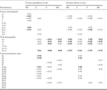
In general terms, the model was more sensitive to parameters controlling tick demography than to those controlling grouse demography or viral transmission coefficients (Table A1). Only for site M1, where the grouse population was low and seroprevalence was high, was there a consistent influence of grouse demographic parameters and their interactions. However, for site C, the effect of increasing the pathogen-induced death rate (α) was to increase the grouse population; although this appears counter-intuitive, it arises because the increased death rate leads to a lower tick infection rate and hence lower numbers of grouse infected and a higher equilibrium grouse density.
Significant effects (Pearson's correlation coefficient, P<0·01) of varying one-patch model system parameters (Table 2) by up to ±1%, including first-order interactions (parameter1×parameter2) within parameter groups (grouse demography, tick demography, viral transmission rates), on the equilibrium grouse population and seroprevalence at 4 study sites reported by Gilbert et al. (Reference Gilbert, Norman, Laurenson, Reid and Hudson2001)
(Bold: accounts for >20% of the variance in the response.)

The model outputs were sensitive to tick demographic parameters at all sites with the exception of the low equilibrium grouse population at site M1. In particular, there were consistently high correlations between model outputs and the interaction between tick death rates and the density-dependent constraint. Viral transmission parameters only had a substantial effect for site C, where there were no hares and very low infection of grouse.
Magnitude of sensitivity to parameters
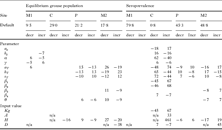
Varying the 3 grouse demographic parameters b g, α and γ had slightly disproportionate effects on the equilibrium grouse population at site M1, where it was low and seroprevalence was high, but otherwise the effects of all grouse demographic parameters were less than proportional (Table A2). The apparently extreme effects of all parameters on seroprevalence at site C are in fact trivial, as its equilibrium value was less than 1%, and any small variation is proportionally large.
The percentage change in the equilibrium grouse population and seroprevalence at four study sites (not reported if <5%) of individually varying one-patch model parameters (Table 2) and input variables by –5% (decr) and +5% (incr). K g grouse carrying capacity, A grouse immigration rate, H hare density, D red deer density
(n/a – default input was zero and could not be decreased – the corresponding increases were A=0·20 and H=1 at site C, D=1 at sites M1 and M2.)
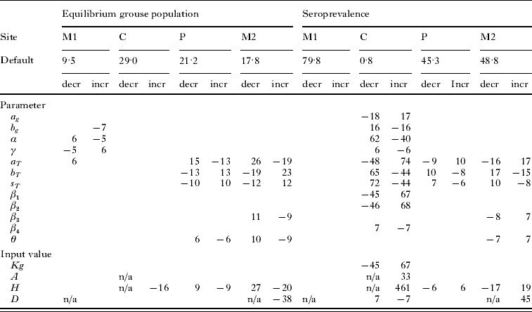
At sites P and M2, all three tick demographic parameters had substantially disproportionate effects on the outputs, particularly at M2, possibly because the grouse carrying capacity was lower or the hare density was higher (or both). Likewise, the effect of varying the non-viraemic transmission coefficient θ was disproportionally high for sites P and M2, but the rate at which adult ticks bite hares and reproduce, β3, had a disproportional effect only at M2. Although the tick-grouse transmission coefficients (β1 and β2) had highly significant effects on the grouse population at site C (Table A1), they were of negligible magnitude (Table A2), presumably because the population was constrained by being close to its carrying capacity.
Magnitude of sensitivity to model inputs
The model was relatively insensitive to changes in the grouse carrying capacity for 3 of the 4 reference sites (Table A2). The exception was for site C, where the very low seroprevalence, but not the grouse population, showed a highly disproportionate response. A similar result was observed for the grouse immigration rate.
In contrast, the model exhibited considerable sensitivity to the densities of hares and deer, especially when hares were increased from zero to 1 km−2 at site C and when deer were increased likewise at site M2, although that was not so at site M1. This sensitivity to a very low host density was apparent not only in terms of increased seroprevalence, but also in substantially reduced grouse populations. These responses merit further investigation, as distinguishing reliably between a very low density and a true absence of a mammalian host over substantial spatial areas in the field can be very difficult, if not impossible.
Changes in hare density of 5% led to moderate changes in the equilibrium grouse population and seroprevalence for site P, and substantial changes for site M2. However, varying the low deer population at site P had very little effect.