Introduction
In recent times, several kinds of pulsed Doppler radio frequency (PDRF) sensor systems have received much attention from researchers because of their wide variety of applications such as long-distance RFID (radio frequency identification) readers, air traffic control [Reference Ghadaki and Dizaji1], meteorology [Reference Doviak, Zrnic and Sirmans2], airborne radio frequency (RF) seekers [Reference Björklund3] and many more. The fundamental working principle of any RF sensor is to detect a target radar cross section (RCS) by means of transmitting RF signal and receiving return signal that consists of target properties and clutter spectral spread. Spectral purity of transmitted signal primarily used to be imperative constraint that limits attainable performance of PDRF sensor applications. In addition to that, spectral spread of clutter returns also degraded phase noise also contributes in raising overall system noise floor. Stage wise signal phase noise flow of pulsed Doppler (PD) radar transmit or receive (Tx/Rx) mode in presence of thermal noise and clutter is discussed in [Reference Leeson4–Reference Robbins6]. Realization of lower phase noise at close-in frequency offsets around fundamental carrier is a tedious task limited by material technology. Phase noise level at close-in frequency offsets is crucial factor in processing of signal flooded with clutter for slow-moving targets and “tail chase” mode in airborne radar applications [Reference Aubry, Carotenuto and Farina7]. Therefore, research on minimization of these stringent low frequency offsets phase noise specifications via signal processing or advanced modeling without compromising system performance is always a challenging task.
Over the years, there have been multiple attempts to model the different aspects of the RF sensor design. The derivation of phase noise theory and a design equation for the phase noise level in PD radar is discussed in [Reference Leeson4, Reference Guo5]. The development of a new design equation for the phase noise level in frequency‐modulated continuous wave (FMCW) radar and its validation with real data is reported in [Reference Siddiq, Watson, Pennock, Avery, Poulton and Martins8]. In previous works dealing with the phase noise analysis of PDRF sensor, the aspects of range correlation effect and inline flicker contribution on residual phase noise is either ignored, or treated in a very implementation-oriented fashion [Reference Li, Wan, Miao and Yang9]. Droitcour et al, analyzed interrogation range of an UHF RFID system based on measurements of the range correlation effect of the transmitter’s leakage signal [Reference Droitcour, Lubecke, Lubecke, Lin and Kovacs10]. However, it does not improve system performance and provide accurate phase noise modeling. A signal level simulator consisting of algorithms for the simulation of raw radar return signals is discussed in [Reference Beasley11, Reference Mikhemar, Murphy, Mirzaei and Darabi12].
Present literature lacks a highly accurate RF sensor phase noise modeling method, which considers both actual operational scenario and design architecture together. Generally, phase noise requirements in wireless communication systems are expressed derivatively by a reciprocal mixing process of interference signal [Reference Mikhemar, Murphy, Mirzaei and Darabi12–Reference Siddiq, Hobden, Pennock and Watson15]. However, for PDRF sensors based on principle of reciprocal mixing phase noise it must get model by considering aspects of phase-noise reduction at lower frequency offsets using range correlation effect and precise inclusion of inline flicker contribution. To the best of our knowledge, there have been no past reports about range correlation effect in reciprocal mixing and inline components flicker contribution in modeling PDRF sensor’s phase noise requirements. The proposed work eliminates the limitations of conventional phase noise modeling for RF sensor. In this article, a qualitative work has been carried out to analyze oscillator’s phase noise modeling used for airborne PDRF sensor in look down mode application with its experimental validation. This work also covers practical design example of a PDRF sensor phase noise requirement using improved modeling in comparison with conventional approach. It offers benefit in reduction of stringent phase noise specifications by using range correlation effect and precise inclusion of inline flicker contribution. This work can be used for mitigating phase noise degradation at close-in frequency offsets due to platform motion or unintentional cause.
The section “Theoretical background” describes range correlation effect, spectral of flicker noise and phase noise in PDRF sensor. Section “Phase noise modeling” explains theoretic approach to model the phase noise of airborne PD radar in lookdown mode considering both range correlation based reciprocal mixing and precise inclusion of inline flicker noise contribution. Section “Experimental investigation of the proposed modeling” covers the experimental verification along with linking its valuable applicability. Finally, at last section “Conclusion” concludes the proposed work.
Theoretical background
Pulsed Doppler RF sensor
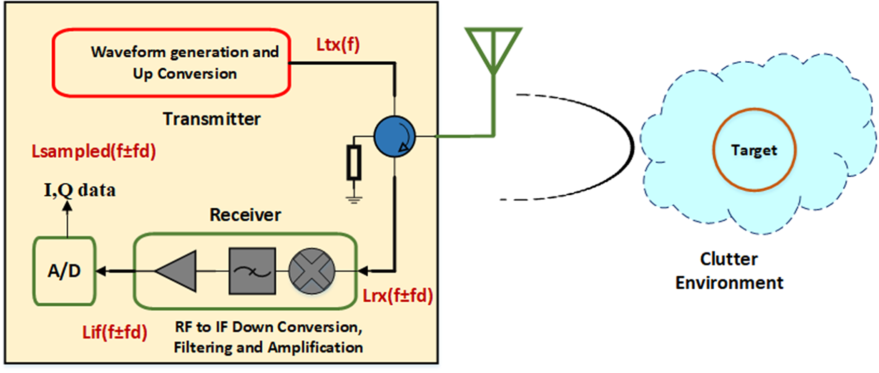
In PDRF sensor, a local oscillator (LO) is normally used for purpose of signal frequency translation in transmit mode and down-conversion operation during receive mode. During receive mode, the phase noise of the received signal is correlated with that of the LO signal. Sequential flow of phase noise analysis in PD sensor Tx/Rx mode signal flooded with noise/clutter environment is shown in Fig. 1.
Flow of phase noise analysis in pulsed Doppler RF sensor transmit and receive mode signal flooded with noise and clutter environment.

Range correlation and inline flicker
Generally, correlation level is inversely proportional to the time difference between the transmitted and received signals in RF sensor. Range-correlation phenomenon in PDRF sensor describes the method to reduce amplitude and phase noise variance which affects the baseband noise spectrum after reciprocal mixing. In PD radar track mode, round around time difference is very small (few nano-sec). Due to this phase noise because of synchronization in coherent receiver will reduce the power spectral density (PSD) dramatically.
Flicker noise is a type of electronic noise which characteristically has a Gaussian distribution and is time-irreversible. Phase noise for bandwidth (B) in Hz at any carrier offset  ${f_0}$+
 ${f_m}$ produces a phase deviation, given by [Reference Robbins6].
 \begin{equation}\Delta {V_{RMS}} = \frac{1}{{\sqrt 2 }}\sqrt {\frac{{FkBT}}{{{P_{av}}}}} \end{equation}
where Δ ${V_{RMS}}$ is RMS value of voltage of the flicker noise, T = Temperature (degree kelvin), B = bandwidth (Hz),
 ${P_{av}}$ = average power in resonator, F = Noise factor and k = Boltzmann constant. Equation (1) can be written as
 \begin{equation}{S_v}\left( {{f_m}} \right) = \Delta V_{RMS}^2 = {{{\text{FkTB}}} \mathord{\left/
{\vphantom {{{\text{FkTB}}} {{P_{av}}}}} \right.
} {{P_{av}}}}\end{equation}
 ${S_v}$(
 ${f_m}$) is spectral purity of the carrier affected by the device generated flicker noise at frequencies close to the carrier frequency and shows a 1/f component with a corner frequency as
 ${f_c}$. The spectral phase noise can be defined as follows [Reference Ghadaki and Dizaji1].
 \begin{equation}{S_v}\left( {{f_m}} \right) = \frac{{FkTB}}{{{P_{av}}}}\left( {1 + \frac{{{f_c}}}{{{f_{}}}}} \right)\end{equation}
where f c = Flicker corner frequency (Hz) and  ${f_m}$= carrier frequency offset (Hz)
In PDRF sensor design architecture, there is an additional effect of additive inline flicker noise (in signal flow path) from active components (i.e. amplifier, mixer, detector etc.) riding on basic oscillator phase noise that further gets translates to final transmitter signal. Phase noise degradation due to additive inline flicker at particular frequency offsets  $\Delta {L^\prime}$(
 ${f_{offset}}$) needs to be considered for improved modeling of operational requirements [Reference Beasley11, Reference Mikhemar, Murphy, Mirzaei and Darabi12].
Phase noise in pulsed Doppler radar
The phase noise at the input to an amplifier in case of oscillator is likely to be bandwidth limited and determined by the quality factor (Q) of the resonator ( ${\omega _0}$), which can be modeled as an amplifier with feedback. Closed loop response of the phase feedback is given by (4) [Reference Robbins6, Reference Hajimiri and Lee13].
 \begin{equation}\Delta {V_{out}}\left( {{f_m}} \right) = \left( {1 + \frac{{{\omega _0}}}{{j2{Q_l}{\omega _m}}}} \right) \cdot \Delta {V_{in}}\left( {{f_m}} \right)\end{equation}
where Δ ${V_{out}}$ is closed loop output signal voltage flicker, Δ
 ${V_{in}}$ is input signal voltage fluctuations in feedback loop.
The power transfer becomes the phase spectral density
 \begin{equation}{S_{out}}\left( {{f_m}} \right) = \left[ {1 + \frac{1}{{f_m^2}}{{\left( {\frac{{{f_0}}}{{2{Q_l}}}} \right)}^2}} \right] \cdot {S_{in}}\left( {{f_m}} \right)\end{equation}
Finally,
 \begin{equation}L\left( {{f_m}} \right) = \frac{1}{2}\left[ {1 + \frac{1}{{f_m^2}}{{\left( {\frac{{{f_0}}}{{2{Q_l}}}} \right)}^2}} \right] \cdot {S_{in}}\left( {{f_m}} \right)\end{equation}
or
 \begin{equation}L\left( {{f_m}} \right) = \frac{1}{2} \cdot \left[ {1 + \frac{1}{{f_m^2}}{{\left( {\frac{{{f_0}}}{{2{Q_l}}}} \right)}^2}} \right] \cdot \frac{{FkTB}}{{{P_{av}}}} \cdot \left( {1 + \frac{{{f_c}}}{{{f_m}}}} \right)\end{equation}
Here,L(f m) = phase noise level (dBc/Hz) at carrier frequency offset ( ${f_m}$)
 ${Q_l}$ = loaded quality factor (Q)
f0 = carrier frequency (Hz)
Finally, equation (7) leads to the Leeson equation for single sided phase noise density in dBc/Hz [Reference Björklund3].
 \begin{align}L\left( {{f_m}} \right) &= 10\,Lo{g_{10}}\left\{ {\frac{{FkT}}{{2{P_{av}}}} \,{\cdot}\, \left[ {1 + \frac{{{f_c}}}{{{f_m}}} + {{\left( {\frac{{{f_0}}}{{2{f_m}{Q_l}}}} \right)}^2} \,{\cdot}\, {\text{ }}\left( {1 + \frac{{{f_c}}}{{{f_m}}}} \right)} \right]} \right\}\nonumber\\ &\quad\times {\text{dBc}}/{\text{Hz}}\end{align}
It may be noted that although the equation (8) indicates an increment in noise density below the cutoff frequency (fc) of 6 dB/octave, some devices may have a greater exponential characteristic, e.g., fc2, with 12 dB/octave or greater increment in noise density below the cutoff frequency.
In the next section, first reciprocal mixing effect without range correlation is examined, and derived typical phase noise equation. Then, a modified phase noise equation considering range correlation and inline flicker contribution effect is derived in PD radar system.
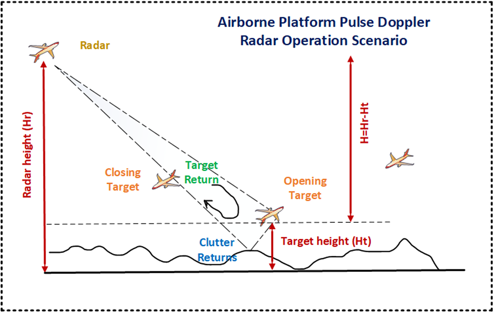
The simplest method for calculating the phase noise for a general communication system is to use reciprocal mixing with adjacent interference signal [Reference Doviak, Zrnic and Sirmans2]. PD radar receiver are typically designed to maximize the target return signal strength and minimize the clutter, resulting in a signal-to-clutter ratio (SCR) adequate for detection and tracking of intended targets. SCR is the ratio of the power received from target RCS to power received from clutter (stationary objects or foliage). Explanatory representation of target tracking scenario (in tail chase mode) in presence of collocated target and clutter is shown in Fig. 2. For an airborne PD radar, operation in “look down” mode at targets above a surface (ex: floor of a desert) having reflectivity characteristics and area confined, SCR can be defined as (9) [Reference Guo5, Reference Aubry, Carotenuto and Farina7].
 \begin{equation}SCR = \frac{{{\sigma _t}}}{{\left[ {\frac{{{\sigma ^0} \cdot \left( {R \cdot \theta } \right) \cdot \left( {C{\text{ }} \cdot \Gamma } \right)}}{2} \cdot \sec \left( \varphi \right)} \right]}}\end{equation}
where  ${\sigma _t}$ = target radar cross section
Airborne RF sensor tracking (look down mode) scenario with target in presence of co-located clutter.

 ${\sigma ^0}$ = clutter average reflectivity
R = target range
 $\theta $ = beam width (in degree)
 $\Gamma $ = pulse width
 $\varphi $ = depression angle.
For such operational scenario, the required single side band (SSB) phase noise at any offset frequency of interest can be found using equation (10). Here, the phase noise is assumed to be flat across the band of interest at a certain offset frequency (Δfc) from the carrier.
 \begin{equation}L\left( {{f_{offset}}} \right) = {\text{SCR}}\left( {{\text{dB}}} \right)\,{\text{ - }}\,{B_d}\left( {{\text{dBHz}}} \right)\,{\text{ - }}\,{\text{SI}}{R_{reqd}}\left( {{\text{dB}}} \right)\end{equation}
where  ${B_d}$ = Doppler filter bandwidth (dBHz)
SI ${R_{reqd}}$ = signal to interference required (dB)
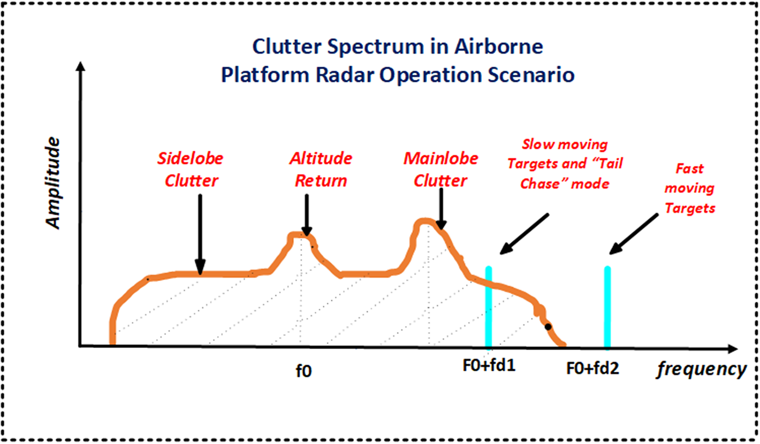
Plugging in the corresponding system requirement values in the equation (10) results in a phase noise requirement of minimum L dBc/Hz down at any Doppler frequency of interest. Airborne radar received signal spectrum consisting of target (in slow moving condition or “tail chase” mode) along with clutter and leakage is shown in Fig. 3.
Clutter spectrum competing with reflected target signal.

The spectrum at a moving platform receiver is different from ground applications because of the relative velocity of the platform ( ${f_0} = \frac{{2{v_p}}}{\lambda }$) to the interceptor, but the same components are present. The time-gating of the pulsed radar can be combined with the frequency discrimination of a CW Doppler to reduce the effects of leakage. Basic transmitted signal of radar system, A(t) can be represented by equation (11) [14].
 \begin{equation}\begin{array}{*{20}{c}}
{A\left( t \right) = {A_0} \cdot {\text{ }}{e^{ - j\left( {2\pi {f_0}t + \varphi \left( t \right)} \right)}}\,{\text{or}}} \\
{{A_0} \cdot {\text{ }}\cos \left( {2{{\pi }}{f_0}t + \varphi \left( t \right)} \right)}
\end{array}\end{equation}
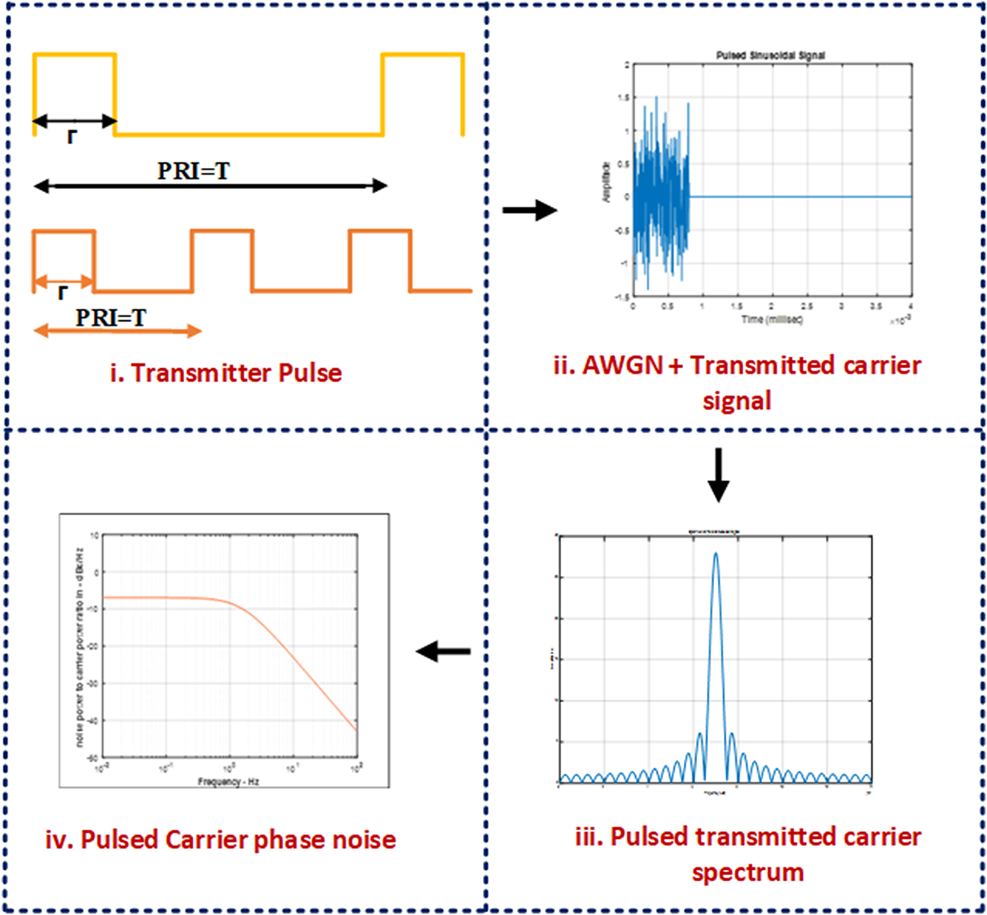
where  ${f_0}$ is the transmitter carrier frequency and φ(t) is a random phase perturbation that is referred to as the phase noise on the carrier signal. Transmitted signal suffers from phase noise and white Gaussian noise (AWGN) level dependent on the system bandwidth. PRI controlled pulsed sinusoidal signal having AWGN and phase noise characteristics as shown in Fig. 4 will be transmitted via impedance transforming device to the environment. Noisy characteristics of transmitted signal getting back scatter by target RCS and unwanted high level clutter strength produces target processing challenging in spite of having time gating advantage.
RF sensor carrier (pulse) anguish with additive white Gaussian noise (AWGN) and phase noise.

Phase noise modeling
Range correlation relation with variance
As mentioned earlier, range-correlation phenomenon in PD radar describes the method to reduce amplitude and phase noise variance which affects the baseband noise spectrum. A quantitative characterization of the relation between range and phase noise can be done in the frequency domain in term of PSD. Variance ( ${\sigma ^2}$) as a measure of dispersion is more preferred to algebraic manipulation than other measures of dispersion such as the expected absolute deviation. The variance can also be thought of as the covariance of a random variable A with itself, or symbolically as
 ${\sigma ^2}$ as shown in equation (12) [Reference Siddiq, Hobden, Pennock and Watson15, Reference Kulpa16].
 \begin{equation}{\sigma ^2} = \operatorname{var} \left( {\text{A}} \right) = {\text{Cov}}\left( {{\text{A,}}\;{\text{A}}} \right)\end{equation}
Variance of a random variable is the expected value of the squared deviation from the mean of A,
 \begin{equation}{{\mu }} = {\text{E}}\left[ {\text{A}} \right]\end{equation}
 \begin{equation}{\text{Var}}\left( {\text{A}} \right) = {\text{E}}\left[ {{{\left( {{\text{A}} - {{\mu }}} \right)}^2}} \right]\end{equation}
 \begin{equation}\begin{aligned}
{\text{Var}}\left( {\text{A}} \right) &= {\text{E}}\left[ {{{\left( {{\text{A}} - {\text{E}}\left[ {\text{A}} \right]} \right)}^2}} \right] \\
& = {\text{E}}\left[ {\left( {{A^2} - 2 \cdot A \cdot E\left[ A \right] + {\text{E}}{{\left[ {\text{A}} \right]}^2}} \right)} \right] \\
& = {\text{E}}\left[ {\left( {{{\left[ A \right]}^2} - 2 \cdot {\text{E}}\left[ {\text{A}} \right] \cdot {\text{E}}\left[ {\text{A}} \right] + {\text{E}}{{\left[ {\text{A}} \right]}^2}} \right)} \right] \\
\end{aligned} \end{equation}
 \begin{equation}{\text{Var}}\left( {\text{A}} \right) = {\text{E}}\left[ {{A^2}} \right]\; - \;{\text{E}}{\left[ {\text{A}} \right]^2}\end{equation}
Reciprocal mixing
Mixing operation is unique with respect to phase noise analysis because they have typically two or more input signal frequencies. Reciprocal mixing may cause the receiving system to lose sensitivity when there is a strong signal near the frequency of “tail chase” mode airborne encounter (air to air). The effect is due to the phase noise of the LO modulating the carrier of the strong signal. The carrier is spread in frequency by the phase noise modulation, which results in a PSD that is proportional to the LO’s SSB phase noise. When the receiver is tuned to a frequency near the strong carrier, the power density in the strong carrier’s noise sidebands may exceed the noise floor of the receiver. If it does exceed the noise floor, then the receiver sensitivity is limited by reciprocal mixing [Reference Cooper17, Reference Rezaei and Mohammadpour18].
Product of statistically dependent variables
If two variables A and B are statistically dependent, then the variance of their product is given by equation (17):
 \begin{equation}\begin{gathered}
{\text{Var}}\left( {{\text{AB}}} \right) = {\text{E}}\left[ {{A^2}{B^2}} \right] - {\text{E}}{\left[ {\left( {{\text{AB}}} \right)} \right]^2} \\
= {\text{Cov}}\left( {{A^2},{B^2}} \right) + {\text{E}}\left( {{A^2}} \right) \cdot {\text{E}}\left( {{B^2}} \right) - {\text{E}}{\left[ {\left( {{\text{AB}}} \right)} \right]^2} \\
= {\text{Cov}}\left( {{A^2},{B^2}} \right) + \left( {\text{Var}}\left( {\text{A}} \right) + {\left[ {{\text{E}}\left( {\text{A}} \right)} \right]}^{2} \right) \cdot \big( {\text{Var}}\left( {\text{B}} \right) \\ + {{\left[ {{\text{E}}\left( {\text{B}} \right)} \right]}^2} \big) - {\left[ {{\text{Cov}}\left( {{\text{A,B}}} \right) + {\text{E}}\left( {\text{A}} \right){\text{E}}\left( {\text{B}} \right)} \right]^2} \\
\end{gathered} \end{equation}
Similarly, multiplication of statistically dependent variables variances in receiver of LO and received echo in PD radar leads to the product of noise spectral surrounded by the LO and reflected signal.
Multiplication of variances in non-coherent signals
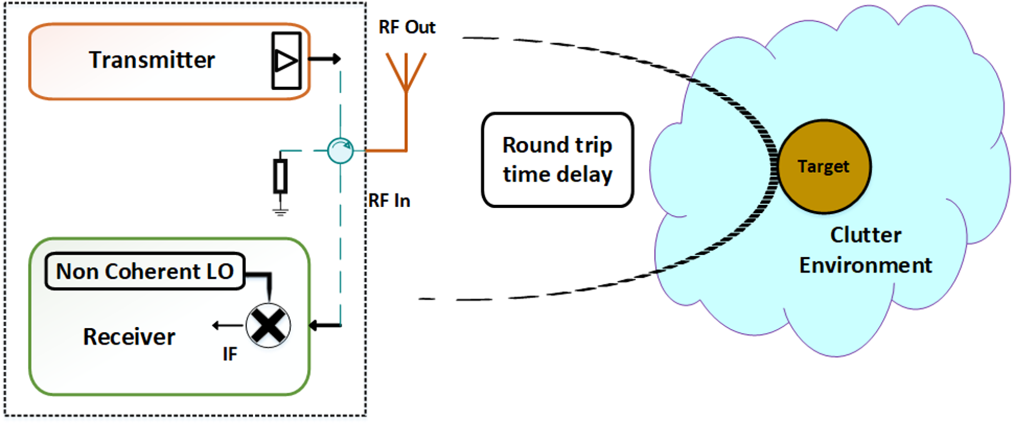
Simplest PD radar system can be described in three simple blocks transmitter/receiver section, target, and environmental channel. If LO in receiver is non-synchronized with transmitter signal as situation occurs in non-coherent radar processing, condition will be multiplication of statistically independent variables variances. This mathematical phenomenon in non-coherent heterodyne PDRF sensor architecture is represented in Fig. 5.
 \begin{equation*}Var (AB)=var(A) \,X\, var(B);\text{ }statistically\text{ }independent\text{ } variables\end{equation*}
Non-coherent heterodyne RF sensor operation and processing architecture.

Multiplication of variances in coherent signals
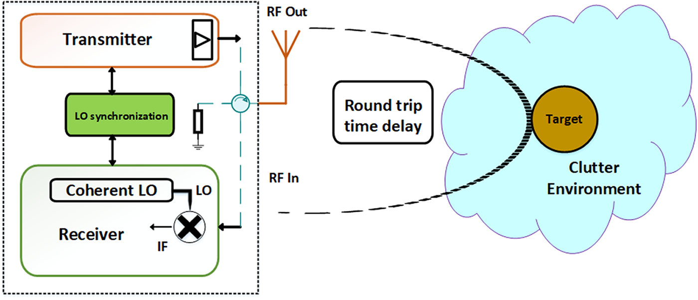
If LO in receiver is synchronized with transmitter signal as situation occurs in coherent radar processing, condition will be multiplication of statistically independent variables variances. This mathematical phenomenon coherent heterodyne PDRF sensor architecture is represented in Fig. 6.
 \begin{equation*}Var (AA)=var(A) \,X\, var(A);\text{ } statistically\text{ } dependent\text{ } variables\end{equation*}
This parameter is related to commonly used phase noise specification. By integrating through the bandwidth of the baseband filter, we can calculate the variance of the phase noise relating to the range correlation effect.
Coherent heterodyne RF sensor operation and processing architecture.

Analysis of time delay reflected echo
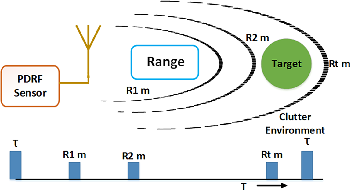
In presence of target within unambiguous range of radar, echo from target will be received on transmitted chain of pulses in different range bins as shown in Fig. 7. If the signal is reflected by a target at a nominal distance d, the received signal can be found by equation (18).
 \begin{equation}R\left( t \right) = {A_d}\left( t \right) \cdot \cos \left( {2\pi f({\text{t}} - \frac{{2d}}{c}) + \varphi ({\text{t}} - \frac{{2d}}{c})} \right)\end{equation}
where R(t) is the back-scattered signal of the target from range d meter and φ (t −  $\frac{{2d}}{c}$) is phase change due to round trip delay.
Round trip delayed signals in range bins during receive ‘ON’ time.

The received signal is multiplied by a LO signal that is derived from the same source as the transmitted signal. When the received and LO signals are mixed in receiver, the output becomes a low-pass filtered signal. The resulting baseband signal is represented by equation (19).
 \begin{equation}{R_{info}}\left( t \right) = {A_d}\left( t \right) \cdot \cos \left( {\frac{{4\pi d}}{\lambda }) + \Delta \varphi ({\text{t}})} \right)\end{equation}
where Δφ(t) = φ(t) − φ (t −  $\frac{{2d}}{c}$) is the residual phase noise.
Range-correlation in receiver describes the method to residual phase noise ∆φ(t) which affects the baseband noise spectrum. The corresponding phase noise can be expressed as described in equation (20).
 \begin{equation}{L_{\Delta \varphi }}(\Delta {f_c}) = L(\Delta {f_c}).[4si{n^2}(2\pi \frac{{d\Delta {f_c}}}{c})]\end{equation}
 \begin{equation}\text{Imp Factor} = 10*\log_{10}(2-2\cos{\left(\frac{{4\pi R\Delta {f_c}}}{c}\right)})\end{equation}
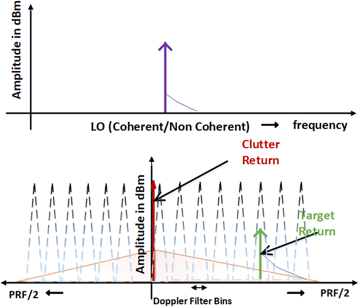
Imp Factor in Equation (21) suggests significant advantage at lower offsets frequency. At larger offset frequency, the signal purity can be achieved easily. Advantage of accurate phase noise modeling in low offset frequencies demands clock synchronization and system coherency. This is crucial factor in processing of slow-moving targets with closer Doppler offsets and “tail chase” mode encounters in airborne applications flooded with clutter cloud. Doppler processing in presence of clutter backscatters in coherent or non-coherent condition is shown in Fig. 8.
Doppler processing in presence of clutter backscatters.

Improvement factor in low offset frequency range is achieved through range correlation in coherent receiver topology. The improvement factor helps to relax the requirement of stringent phase noise specifications. Equation (10) can be reconfigured to account improvement factor in close in offsets to redefine needs as described in equation (22). At higher offsets beyond 1 KHz phase coherency perishes down and same is verified through experimentation in section 4.
 \begin{align}
L'({f_{offset}}) & = {\text{SCR(dB)}} - {B_d}({\text{dBHz}}) - {\text{S}}{{{IR}}_{{{reqd}}}}({\text{dB}}) \nonumber \\
& \quad + 10 Log_{10}{\text{ }}\left(2 - 2\cos\left(\frac{{4\pi R\Delta {f_c}}}{c}\right)\right) \nonumber \\
& \;\;\;\;\;\;\;:\left\{ {\Delta {f_c} \leq 1KHz} \right\}\nonumber \\
& = {\text{SCR\,(dB)}} - {B_d}\,\left({\text{{dBHz}}} \right) - \text{SI}{R_{reqd}}\,\left( {dB} \right)\nonumber \\
& \;\;\;\;\;\;\;:
\left\{ \Delta {f_c} \gt 1KHz\right\} \end{align}
where  $L{^{\prime}}$(foffset) is the phase noise level (dBc/Hz) at carrier frequency offset within
 ${B_d}$.
 ${B_d}$ = Doppler filter bandwidth (dBHz)
SI ${R_{reqd}}$ = Signal to interference required (dB)
SCR = Ratio of the power received from target to power received from clutter.
Practically in RF sensor design there is additive effects of additive inline flicker noise (in signal flow path) arising from active components (i.e., amplifier, mixer, detector etc.). The flicker noise is superposed on basic oscillator phase noise that further translates to final transmitter signal. Any phase noise degradation due to additive inline flicker at particular frequency offsets  $\Delta {L^\prime}$(
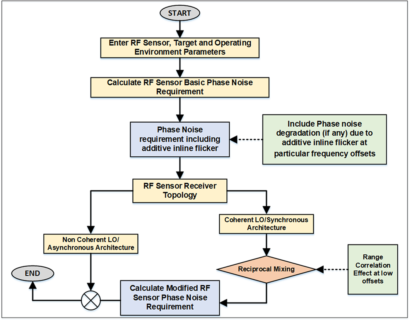
 ${f_{offset}}$) further need to consider while computing overall requirements in agreement with equation (22) as dominant noise signal. Considering the flicker noise the equation (22) is modified which is expressed by equation (23). Complete method flow diagram for calculating modified RF sensor phase noise requirement is shown in Fig. 9.
 \begin{align}
L\prime \left( {{f_{offset}}} \right) & = {\text{SCR}}\left( {{\text{dB}}} \right) - {B_d}\left( {{\text{dBHz}}} \right) - {\text{SI}}{R_{reqd}}\left( {{\text{dB}}} \right) \nonumber \\
& \quad + 10Lo{g_{10}}\left( {2 - 2\cos \left( {\frac{{4\pi R\Delta {f_c}}}{c}} \right)} \right) - \Delta L\prime \left( {{f_{offset}}} \right) \nonumber \\
& \;\;\;\;\;\;\;:\left\{ {\Delta {f_c} \leqslant 1KHz} \right\} \nonumber \\
& = {\text{SCR}}\left( {{\text{dB}}} \right) - {B_d}\left( {{\text{dBHz}}} \right) - {\text{SI}}{R_{reqd}}\left( {{\text{dB}}} \right) - \Delta L\prime \left( {{f_{offset}}} \right) \nonumber \\
& \;\;\;\;\;\;\;:\left\{ {\Delta {f_c} \gt 1KHz} \right\}
\end{align}
Flowchart for calculating modified RF sensor phase noise.

where  $L{^{\prime}}$(foffset) is the phase noise level (dBc/Hz) at carrier frequency offset within
 ${B_d}$.
 ${B_d}$ = Doppler filter bandwidth (dBHz)
SI ${R_{reqd}}$ = Signal to interference required (dB)
 $\Delta {L^\prime}$(
 ${f_{offset}}$) = Phase noise degradation due to additive inline flicker at particular frequency offsets.
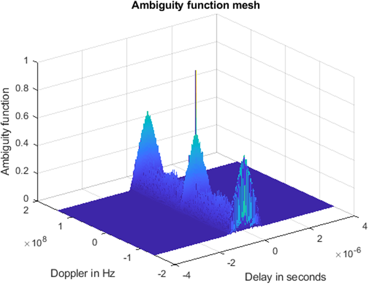
Reflected signal processing in ambiguity function having delayed by time  $\frac{{2d}}{c}$ and shifted in Doppler
 ${f_d}$ is shown in Fig. 10. It represents auto-correlated output used for Doppler information extraction. Information processing demands for high-cost oscillator phase noise requirements in close offsets as per generally used equation (10). Effects of precise and improved modeling taking effects of range correlation together with coherent architecture offers innovative way to model phase noise requirements. This encompasses added advantage in low Doppler offset frequencies (slow moving target processing) without much hardware restrictions and additive active components flicker noise contribution if it dominates in signal flow track at any stage [Reference Ayhan, Scherr, Bhutani, Fischbach, Pauli and Zwick19–Reference Jahangir21].
Ambiguity function of RF sensor’s reflected signal in time-Doppler map.

Vibration phenomenon in system applications causes lattice disturbance in piezoelectric physical components that causes phase variations. In general, the effect is more prominent in higher-frequency oscillators due to increased signal phase sensitivity to mechanical deformation and decreased resonator quality factor. Reference crystal sensitivity to vibration is traditionally characterized by acceleration/vibration sensitivity, which is normalized frequency change per unit gravitational acceleration g. In random vibration test, amplitude of vibration level is defined in terms of PSD. Level shift of phase noise ( $L\left( {{f_v}} \right))\,$at particular offset from fundamental carrier frequency is shown in equation (24) [Reference Howe, Lanfranchi, Cutsinger, Hati and Nelson22–Reference Kumar24].
 \begin{equation}L\left( {{f_v}} \right) = 20 \times log{\text{ }}{\left(\frac{{\bar \Gamma {A_{peak}}{f_0}}}{{2{f_v}}}\right)}{\text{ }}dB\end{equation}
 \begin{equation}\bar \Gamma = \frac{{2.{f_v}}}{{{A_{peak}}.{f_0}}}{10^{\frac{{L\left( {{f_v}} \right)}}{{20}}}}{\text{ }}Hz/g\end{equation}
Here,  $L\left( {{f_v}} \right)$ is level shift of phase noise at particular offset from fundamental carrier frequency,
 ${A_{peak}}$ =
 $\sqrt {2 \times PSD} $ is peak g-sensitivity,
 $\bar \Gamma $ is acceleration sensitivity,
 ${f_o}$ is the fundamental frequency of reference crystal and
 ${f_v}$ is the offset from fundamental frequency.
 $\bar \Gamma $ of any Reference crystal is dependent on PSD and vibration spectrum. It is defined here in (25) [25, Reference Hati, Nelson and Howe26].
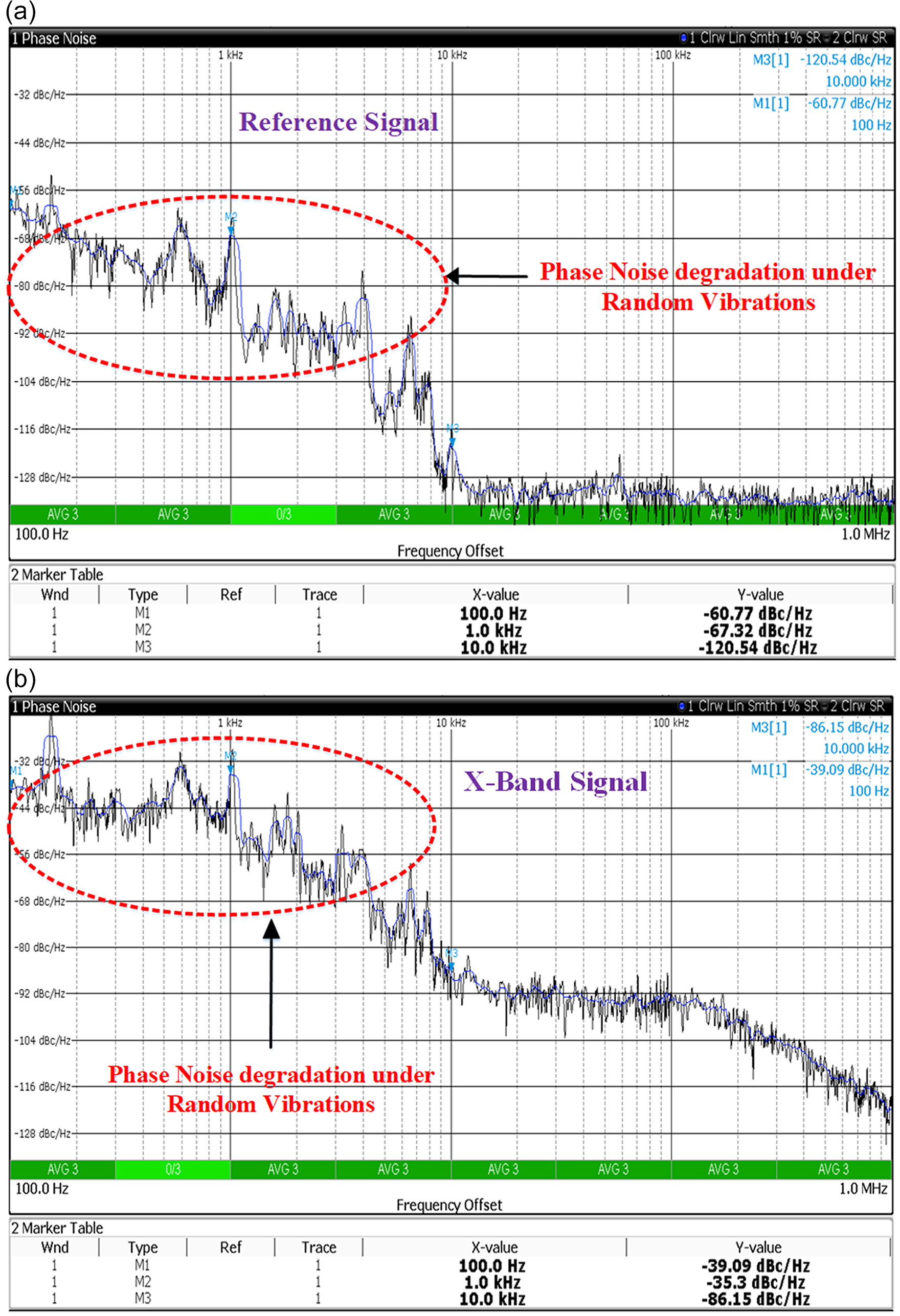
For experimental validation, random vibration test has been carried out with X-band frequency source mounted on shaker using a custom test fixture designed for this purpose. Phase noise performance degradation examined using phase noise measurement application of real-time spectrum (RTS) analyzer under high magnitude random vibration test at low offset frequencies of 100 Hz, 1 KHz and 10 KHz for 100 MHz and X-band signals are shown in Fig. 11(a) and (b) respectively. Phase noise performance significantly degrades under ambient conditions at low offsets of 100 Hz and 1 KHz by ∼50 dBc and ∼45 dBc, respectively. Close in phase noise degradation can be mitigated with utilizing precise phase noise modeling as per equation (23). It helps in meeting stringent requirements in spite of slight degradation due to platform motion and unintentional causes which generally use to be prominent in closer offsets or close to carrier frequency pickups.
Phase noise degradation: (a) basic reference signal, (b) x-band signal.

Experimental investigation of the proposed modeling
Experimental setup description
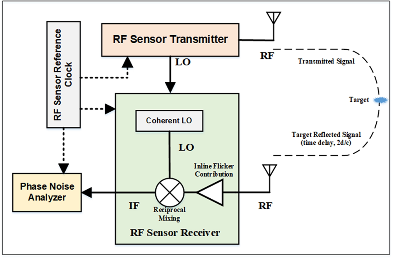
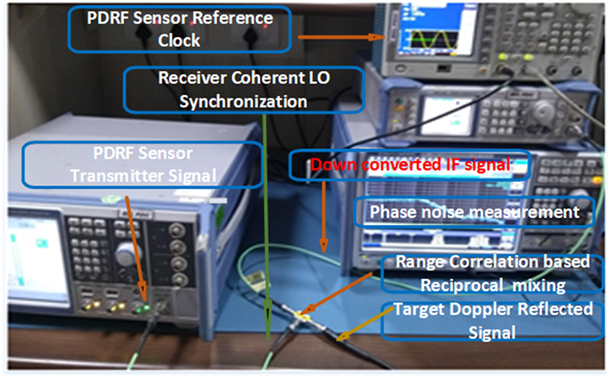
Block diagram of RF sensor test setup illustrating the experimental setup’s key components and signal flow is shown in Fig. 12.
Block diagram of RF sensor phase noise measurement test setup.

Experimental setup with coherence PD radar architecture and operational scenario to study improvement for lower (close in) Doppler offsets is shown in Fig. 13. In this experimental setup LO provides two identical frequency signals, one for the transmitter and the other for the receiver. Assuming that the amplitude noise is so small as to be ignored. The transmitter signal is amplified by power amplifier (PA), feeds into the transmitting antenna, and is radiated into the air. Simultaneously, the receiving antenna also receives backscattered signals from the target. At the receiver, the backscattered signal and the LO signal are mixed, and the output is low-pass filtered.
Practical experimentation and validation of phase noise modeling at lower frequency offsets.

The residual phase noise of the received signal depends on the time delay, 2d/c. When the time delay is short, the correlation effect greatly reduces the noise spectrum at the baseband. The transmitter signal was time delayed using a delay line cable and connected to the MarkiM2H0220LA passive mixer. The LO signal was connected to the LO port of the mixer. The baseband output of the mixer was measured with an FSW43 signal analyzer. To eliminate the dc offset due to transmitter leakage, the phase shifter was tuned until the dc component of the baseband signal, as viewed on an oscilloscope, was zero. The loss through the cables and phase shifter was compensated with inline-amplifier. Demodulation of phase noise effects necessities-controlled condition with adequate filtering to present actual situation.
Measured results and verification of phase noise modeling
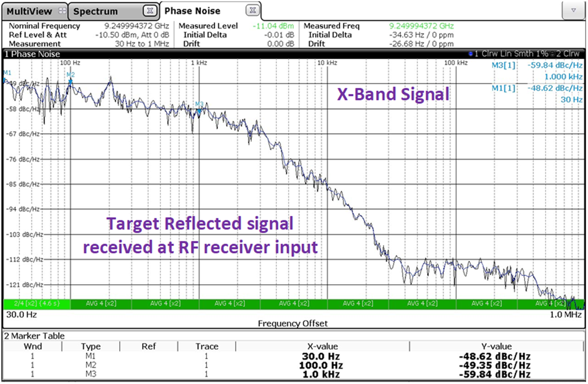
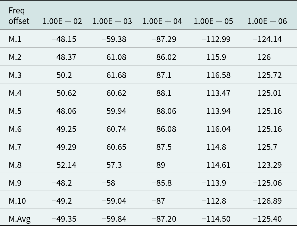
Here, analytical and experimental results of the PD radar system performance considering the range correlation effect on the phase noise are presented. Phase noise measurement requires a significant care due to the low measurement levels and possible interference from the electromagnetic environment. In line with theoretical analysis experimental verification is carried out to support the study. In order to evaluate the phase noise reduction effect caused by the range correlation, the PSD for different offset frequencies is measured and compared with calculated value using (23). Figure 14 presents the measured phase noise of reflected RF signal from desired target and undesired interferences within confined area of illumination. Phase noise can be done in the frequency domain in term of PSD. For consistent statistical measurement, the PSD and Variance ( ${\sigma ^2}$) from 100 Hz to 1 MHz was measured and averaged over ten measurements and has been noted as charted in Table 1. RF phase noise is measured by the conventional method using a RTS phase noise measurement mode.
Monitored phase noise of reflected signal in RF sensor operating environment.

Phase noise variance measurement from 100 Hz to 1 MHz

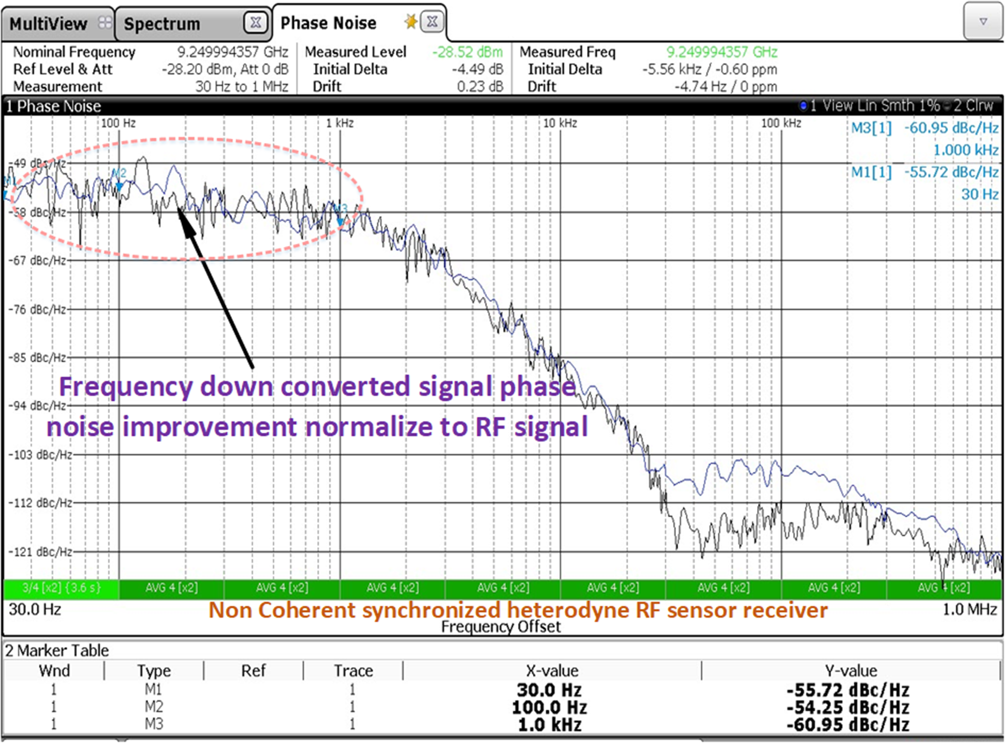
The intended return signal from desired target has to compete with strong stationary clutters or undesired moving targets by factor of  ${R^4}$ due to two-way transmission. Effects of theoretical investigation in regions of close in Doppler processing improvement in under different of receiver condition are monitored. Results are indicative no improvements is occurred if coherency and timing synchronization is not maintained while processing in receiver of radar.
Experimental result of normalized RF to IF of non-coherent time delay reflected echo condition is shown in Fig. 15. In such operating condition added advantage of improved phase noise modeling cannot be utilized effectively. Quantification of additive phase noise degradation or active component flicker contribution over any particular frequency offsets  $\Delta {L^\prime}$(
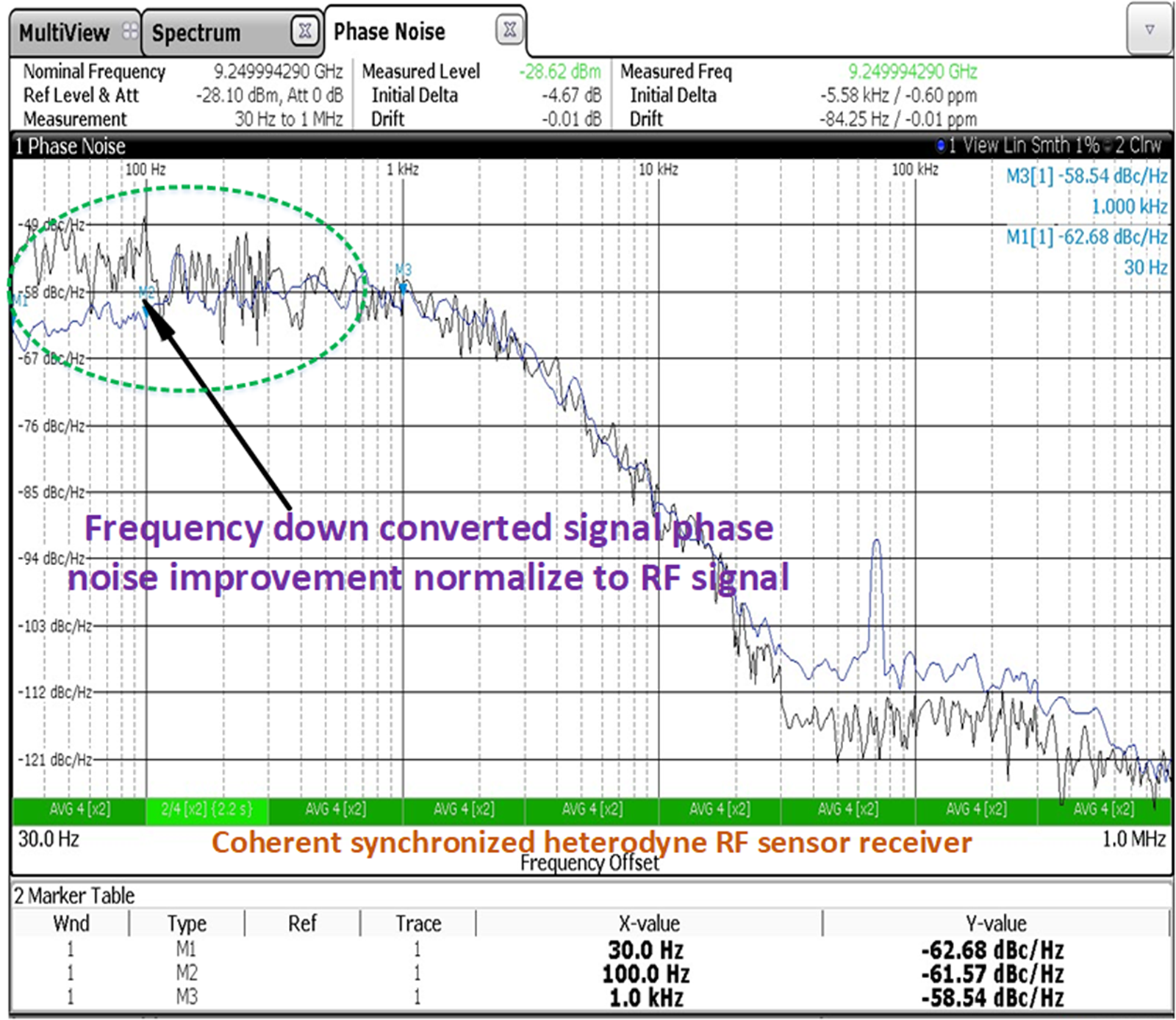
 ${f_{offset}}$) can easily be equated with ideal (expected). Quite good improvement in results is noted if coherency and timing synchronization is properly maintained while processing at receiver. Experimental result of normalized RF to IF of coherent time delay reflected echo condition is shown in Fig. 16 highlighting phase noise improvement in low offset frequencies (lesser than 1 KHz).
Practical experimentation results of phase noise in non-coherent heterodyne RF sensor receiver.

Practical experimentation results of phase noise in coherent synchronized heterodyne RF sensor receiver.

Improved PN modeling comparison with conventional modeling
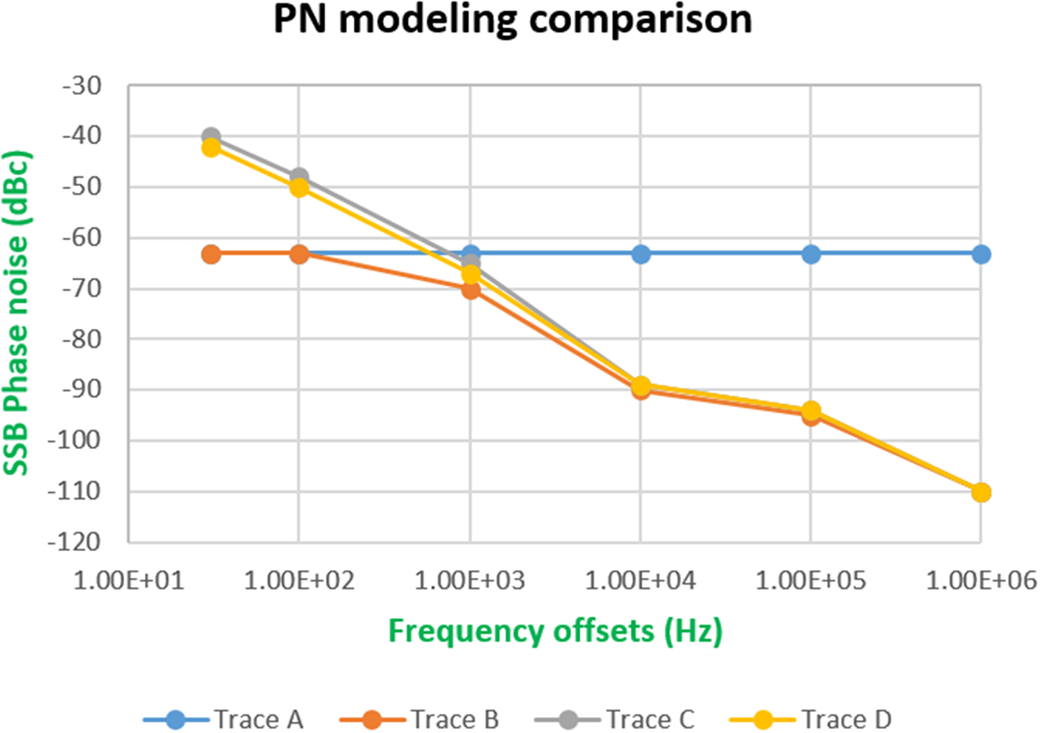
Considering a typical scenario of airborne-PD sensor, with its parameters and operational conditions resulting in SCR of −30 dB typically. For operation dwell time of 10 ms, resultant Doppler filter bandwidth is 100 Hz (20 dBHz). For reliable detection with Pd = 90% and Pfa =  ${10^{ - 6}}$ requires minimum SIR of about 13 dB. Then, the minimum required SSB phase noise at any offset frequency of interest is at least −63 dBc/Hz derived from equation (10) plotted in trace A of Fig. 17 [Reference Leeson4]. As per conventional modeling method, this value must hold at all frequency offsets. As mentioned earlier, realization of ultra low phase noise at close-in frequency offsets around fundamental carrier is a tedious task limit by present material technology available. For a signal source design PLL generated signal phase noise is collectively dependent on PLL, loop filter design, VCO and charge pump. A typical pattern of PLL generated signal source’s phase noise at multiple offsets is plotted in trace B of Fig. 17. As stated and verified, improvement factor at lower frequency offset can be achieved through range correlation in coherent receiver topology. This improvement factor helps to relaxing the stringent phase noise specifications as per equation (21). Equation (10) can be modified to account this improvement factor at close-in offsets and to redefine requirements as per equation (22). At higher offsets beyond 1 KHz phase coherency perishes down and same is verified through experimentation also. Precise SSB phase noise requirement at multiple offset frequencies of interest can be found from equation (22). In agreement with improved and efficient modeling signal phase noise at multiple offsets is plotted in trace C of Fig. 17. Effect of additive inline flicker noise occurring in signal flow path is superposed on basic oscillator phase noise, which finally gets translate to transmitted RF signal. Phase noise degradation due to additive inline flicker at all frequency offsets
 $\Delta {L^{\text{'}}}$(
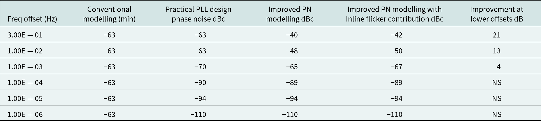
 ${f_{offset}}$) is further considered while computing overall requirements as per equation (23) shown in trace D of Fig. 17. Table 2 Summarizes and compare practical design example of a PLL based signal source requirement using improved phase noise modeling compared with conventional modeling. At higher offsets beyond 1 KHz phase coherency perishes down as per equation (22).
Improved phase noise modeling comparison with conventional modeling.

Signal source phase noise requirement

NS = not significant, PN = phase noise
Work offers benefit in reduction of stringent phase noise specifications by using range correlation effect and precise inclusion of inline flicker contribution. It can be used for mitigating phase noise degradation at close-in frequency offsets due to platform motion or unintentional cause via prior assessment of vibrational environment using equation (24).
Experimental data authenticates proposed phase noise modeling technique. Therefore, proposed precise and accurate phase noise modeling redefines the stringent requirements in PD radar system. It suggests efficient and reliable way of reframing design requirements accounting phase noise degradations due to active flicker if persists dominates in signal flow track at any stage. Figure 16 shows a comparison of theoretical exertion with practical measurement results. Following (9) to (23), we can compute the importance of range correlation effects in defining phase noise requirements in heterodyne based coherent PD RF sensor for defined SCR and additive precise flicker contribution at particular offsets.
Conclusion
Phase noise level at close-in frequency offsets is crucial factor in processing of signal flooded with clutter for slow-moving targets and “tail chase” mode in airborne radar applications. Minimization of these stringent low frequency offsets phase noise specifications via signal processing or advanced modeling without compromising system performance is important. In this study, the effects of range correlation on the phase noise of PDRF sensor signal have been investigated. Precise airborne PD radar phase noise requirement for lookdown mode is modeled considering both range correlation effect during reciprocal mixing and inline components flicker contribution An improved equation has been proposed for accurate phase noise estimation. Improved modeling offers benefit in reducing the stringent RF sensor phase noise specifications at close-in frequency offsets using range correlation effect and precise inclusion of inline flicker contribution. Design example of a PDRF sensor phase noise requirements using improved modeling has been presented. Work can be used to mitigate random vibration effects at close-in phase noise offsets avoiding complex stabilization practices and stringent oscillator design phase noise specification. The proposed model has been experimentally validated also.
Availability of data and material
Authors declare the transparency of the data used in their articles.
Acknowledgements
The authors would like to people who had given valuable suggestions. The authors would like to specially thank Mr. Manjunath R Sr. DGM and Mr. Sivakumar R DGM for support during this work.
Author contributions
All authors contributed to the study's conception, design, circuit preparation, experimentation and draft preparation of the manuscript.
Funding
No funding was received for carrying out this research work.
Conflict of interests
The authors declare that there is no conflict of interests regarding this publication of this article. Necessary permission to publish this article has been obtained from TP/CO department of Bharat Electronics Limited.

Vipin Kumar received B. Tech degree in Electronics and Communication Engineering and M. Tech degree in RF and Microwave Engineering from GGSIPU, New Delhi, India in 2012 and 2015, respectively. He is UGC-NET and GATE qualified. From April 2016, he has been working as RF Design Engineer in Bharat Electronics Limited (BEL) in domain of radar system design engineering, frequency synthesizer and microwave modules for airborne and ground base applications. He has authored technical publications in SCI indexed Journals and reputed IEEE conferences, filed patent and copyright applications at Indian patent office. He is recipient of Best Paper Award in IEEE International Conference on Microwave Integrated Circuits, Photonics and Wireless Networks (IMICPW) 2019 held at NIT Trichy. His current research interests include radar system engineering, RF and microwave circuit design and noise analysis.

Jayanta Ghosh received the M.E. and Ph.D. degrees in electronics and communication engineering from the Birla Institute of Technology, Mesra, India, in 2005 and 2012, respectively. He is currently an Associate Professor with the Department of Electronics and Communication Engineering, National Institute of Technology Patna, India. His research interests include antennas, artificial materials and MICs. He is a senior member of IEEE and Member of IE(I). He is a reviewer of several journals of international repute, i.e., IET Microwaves, Antennas and Propagation, IEEE Antennas and Wireless Propagation Letters, IEEE Transactions on Antennas and Propagation.