2.1 Optimisation problem

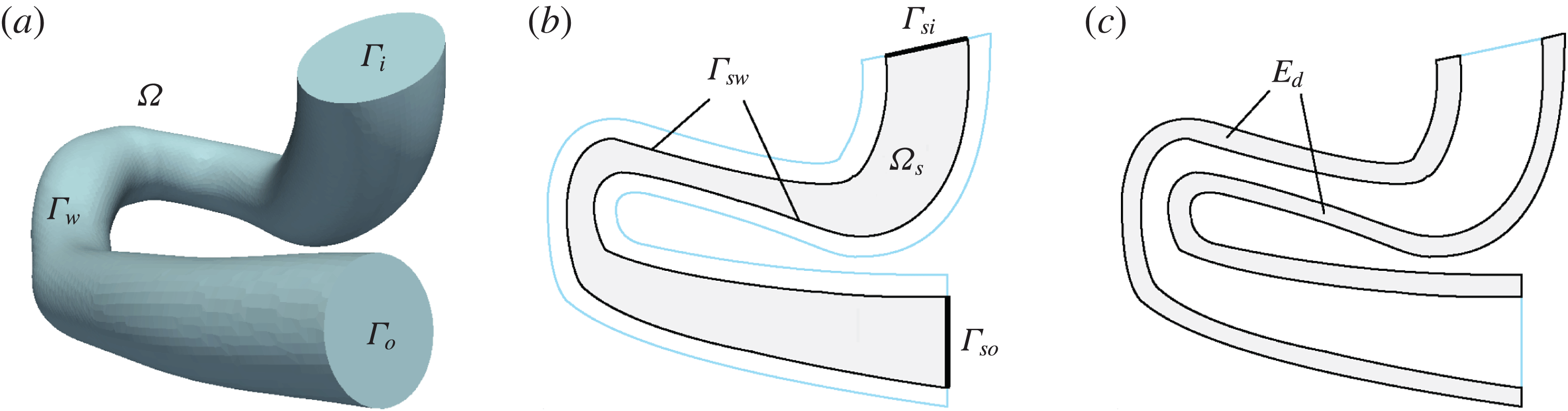
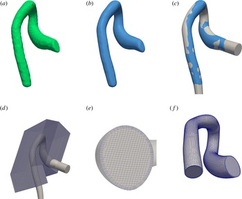
Let us define a bounded Lipschitz domain $\unicode[STIX]{x1D6FA}\subset \mathbb{R}^{3}$ along with its boundary $\unicode[STIX]{x2202}\unicode[STIX]{x1D6FA}=\unicode[STIX]{x1D6E4}_{i}\cup \unicode[STIX]{x1D6E4}_{o}\cup \unicode[STIX]{x1D6E4}_{w}$ , where $\unicode[STIX]{x1D6E4}_{i},\unicode[STIX]{x1D6E4}_{o},\unicode[STIX]{x1D6E4}_{w}\subset \mathbb{R}^{3}$ stand for the inlet, outlet and arterial wall boundaries respectively. Figure 1(a) illustrates such a domain resembling an aortic vascular geometry (to be used later in § 5). We further define a contracted subdomain $\unicode[STIX]{x1D6FA}_{s}\subset \unicode[STIX]{x1D6FA}$ with boundary $\unicode[STIX]{x2202}\unicode[STIX]{x1D6FA}_{s}=\unicode[STIX]{x1D6E4}_{si}\cup \unicode[STIX]{x1D6E4}_{so}\cup \unicode[STIX]{x1D6E4}_{sw}$ , where $\unicode[STIX]{x1D6E4}_{si}\subset \unicode[STIX]{x1D6E4}_{i}$ and $\unicode[STIX]{x1D6E4}_{so}\subset \unicode[STIX]{x1D6E4}_{o}$ (see figure 1 b). The incompressible steady flow of a Newtonian fluid is considered in $\unicode[STIX]{x1D6FA}$ . The inflow at $\unicode[STIX]{x1D6E4}_{i}$ is prescribed by the function $\boldsymbol{g}=\boldsymbol{g}(\boldsymbol{x})\boldsymbol{ : }\unicode[STIX]{x1D6E4}_{i}\rightarrow \mathbb{R}^{3}$ , whereas the density and dynamic viscosity of the fluid are represented by $\unicode[STIX]{x1D70C}$ and $\unicode[STIX]{x1D707}$ respectively. At the outflow, $\unicode[STIX]{x1D6E4}_{o}$ , a traction-free boundary (i.e. a homogeneous Neumann BC) is considered. This hypothesis is exact when the flow is fully developed, and it is physiologically reasonable in the present context. We highlight the fact that the function $\boldsymbol{g}$ is such that $\boldsymbol{g}|_{\unicode[STIX]{x1D6FE}_{i}}=0$ , where $\unicode[STIX]{x1D6FE}_{i}$ is the boundary of surface $\unicode[STIX]{x1D6E4}_{i}$ . In what follows, $L^{2}(\unicode[STIX]{x1D6FA})$ stands for the space of square integrable scalar functions in $\unicode[STIX]{x1D6FA}$ , while $\boldsymbol{H}^{1}(\unicode[STIX]{x1D6FA})$ is the space of square integrable vector functions whose first derivatives are also square integrable functions in $\unicode[STIX]{x1D6FA}$ . The blood flow velocity, , with

(2.1) $$\begin{eqnarray}\boldsymbol{{\mathcal{U}}}^{\ast }=\{\boldsymbol{v}\in \boldsymbol{H}^{1}(\unicode[STIX]{x1D6FA})\mid \operatorname{div}\boldsymbol{v}=0,\boldsymbol{v}|_{\unicode[STIX]{x1D6E4}_{w}}=\mathbf{0},\boldsymbol{v}|_{\unicode[STIX]{x1D6E4}_{i}}=\boldsymbol{g}\},\end{eqnarray}$$

is a solution of the steady-state Navier–Stokes equations, which are written in variational form as follows:

(2.2)

where the strain rate tensor is defined as $\unicode[STIX]{x1D735}^{s}(\cdot )=[\unicode[STIX]{x1D735}(\cdot )+(\unicode[STIX]{x1D735}(\cdot ))^{\text{T}}]/2$ and

(2.3)

Figure 1.

The computational domain. (a) The domain $\unicode[STIX]{x1D6FA}$ along with boundaries $\unicode[STIX]{x1D6E4}_{i}$ , inlet, $\unicode[STIX]{x1D6E4}_{o}$ , outlet, and $\unicode[STIX]{x1D6E4}_{w}$ , wall. (b) The flow-matching domain $\unicode[STIX]{x1D6FA}_{s}\subset \unicode[STIX]{x1D6FA}$ with boundaries $\unicode[STIX]{x2202}\unicode[STIX]{x1D6FA}_{s}=\unicode[STIX]{x1D6E4}_{si}\cup \unicode[STIX]{x1D6E4}_{so}\cup \unicode[STIX]{x1D6E4}_{sw}$ , which is at a distance $s$ (mm) from $\unicode[STIX]{x1D6E4}_{w}$ . (c) The error measurement domain $E_{d}$ , which is within $d$ (mm) distance of $\unicode[STIX]{x1D6E4}_{w}$ .

The constraints $\operatorname{div}\boldsymbol{u}=0$ and $\boldsymbol{u}|_{\unicode[STIX]{x1D6E4}_{i}}=\boldsymbol{g}$ can be relaxed using the corresponding Lagrange multipliers $p$ and $\boldsymbol{r}$ . Further, we introduce the space $\boldsymbol{{\mathcal{U}}}=\{\boldsymbol{v}\in \boldsymbol{H}^{1}(\unicode[STIX]{x1D6FA})\mid \boldsymbol{v}|_{\unicode[STIX]{x1D6E4}_{w}}=\mathbf{0}\}$ and the space $\boldsymbol{H}^{-1/2}(\unicode[STIX]{x1D6E4}_{i})$ , which is the dual space of $\boldsymbol{H}^{1/2}(\unicode[STIX]{x1D6E4}_{i})$ (in the sense given by the pairing $\langle \boldsymbol{r},\boldsymbol{u}\rangle _{\boldsymbol{H}^{-1/2}(\unicode[STIX]{x1D6E4}_{i})\times \boldsymbol{H}^{1/2}(\unicode[STIX]{x1D6E4}_{i})}=\int _{\unicode[STIX]{x1D6E4}_{i}}\boldsymbol{r}\boldsymbol{\cdot }\boldsymbol{u}\,\text{d}\unicode[STIX]{x1D6E4}$ ). The problem (2.2) now becomes

(2.4) $$\begin{eqnarray}\displaystyle & & \displaystyle \mathscr{P}_{\unicode[STIX]{x1D6FA}}:\text{find }(\boldsymbol{u},p,\boldsymbol{r})\in \boldsymbol{{\mathcal{U}}}\times L^{2}(\unicode[STIX]{x1D6FA})\times \boldsymbol{H}^{-1/2}(\unicode[STIX]{x1D6E4}_{i})\text{ such that}\nonumber\\ \displaystyle & & \displaystyle \quad \int _{\unicode[STIX]{x1D6FA}}[\unicode[STIX]{x1D70C}(\unicode[STIX]{x1D735}\boldsymbol{u})\boldsymbol{u}\boldsymbol{\cdot }\hat{\boldsymbol{u}}+2\unicode[STIX]{x1D707}\unicode[STIX]{x1D735}^{s}\boldsymbol{u}\boldsymbol{\cdot }\unicode[STIX]{x1D735}^{s}\hat{\boldsymbol{u}}-p\operatorname{div}\hat{\boldsymbol{u}}-\hat{p}\operatorname{div}\boldsymbol{u}]\,\text{d}\unicode[STIX]{x1D6FA}\nonumber\\ \displaystyle & & \displaystyle \qquad =\int _{\unicode[STIX]{x1D6E4}_{i}}\hat{\boldsymbol{r}}\boldsymbol{\cdot }(\boldsymbol{u}-\boldsymbol{g})\,\text{d}\unicode[STIX]{x1D6E4}+\int _{\unicode[STIX]{x1D6E4}_{i}}(\boldsymbol{r}\boldsymbol{\cdot }\hat{\boldsymbol{u}})\,\text{d}\unicode[STIX]{x1D6E4},\quad \forall \,(\hat{\boldsymbol{u}},\hat{p},\hat{\boldsymbol{r}})\in \boldsymbol{{\mathcal{U}}}\times L^{2}(\unicode[STIX]{x1D6FA})\times \boldsymbol{H}^{-1/2}(\unicode[STIX]{x1D6E4}_{i}).\qquad\end{eqnarray}$$

For the control flow problem, we assume that some observations $\tilde{\boldsymbol{u}}^{t}\in \unicode[STIX]{x1D6FA}$ are available. We want to find a velocity field $\boldsymbol{u}$ such that it better matches the observations and, at the same time, is constrained to be a solution of problem $\mathscr{P}_{\unicode[STIX]{x1D6FA}}$ . In what follows, $\unicode[STIX]{x1D735}_{\unicode[STIX]{x1D749}}$ denotes the surface gradient, whereas $\unicode[STIX]{x1D6FD}$ and $\unicode[STIX]{x1D6FD}_{1}$ are arbitrary parameters for a Tikhonov regularisation and $\unicode[STIX]{x1D6FC}$ is a positive real number. The parameters $\unicode[STIX]{x1D6FC}$ , $\unicode[STIX]{x1D6FD}$ and $\unicode[STIX]{x1D6FD}_{1}$ will often be denoted as optimisation parameters. Based on a user-defined cost function, $\mathscr{O}$ , the aforementioned flow-matching problem can be cast as a mathematical optimisation problem, which reads as

(2.5) $$\begin{eqnarray}\displaystyle & & \displaystyle \mathscr{P}_{M}:\text{ find }\boldsymbol{g}\text{ that minimises }\mathscr{O}(\boldsymbol{g})=\mathscr{O}^{\ast }(\boldsymbol{u}(\boldsymbol{g}),\boldsymbol{g},\tilde{\boldsymbol{u}}^{t})\text{ such that }\mathscr{P}_{\unicode[STIX]{x1D6FA}}\text{ holds, where}\nonumber\\ \displaystyle & & \displaystyle \mathscr{O}(\boldsymbol{g})=\frac{\unicode[STIX]{x1D6FC}}{2}\left(\int _{\unicode[STIX]{x1D6FA}_{s}}|\boldsymbol{u}(\boldsymbol{g})-\tilde{\boldsymbol{u}}^{t}|^{2}\,\text{d}\unicode[STIX]{x1D6FA}+\int _{\unicode[STIX]{x1D6E4}_{si}}|\boldsymbol{u}(\boldsymbol{g})-\tilde{\boldsymbol{u}}^{t}|^{2}\,\text{d}\unicode[STIX]{x1D6E4}+\int _{\unicode[STIX]{x1D6E4}_{so}}|\boldsymbol{u}(\boldsymbol{g})-\tilde{\boldsymbol{u}}^{t}|^{2}\,\text{d}\unicode[STIX]{x1D6E4}\right)\nonumber\\ \displaystyle & & \displaystyle \quad \qquad +\,\frac{\unicode[STIX]{x1D6FD}}{2}\int _{\unicode[STIX]{x1D6E4}_{i}}|\boldsymbol{g}|^{2}\,\text{d}\unicode[STIX]{x1D6E4}+\frac{\unicode[STIX]{x1D6FD}_{1}}{2}\int _{\unicode[STIX]{x1D6E4}_{i}}|\unicode[STIX]{x1D735}_{\unicode[STIX]{x1D749}}~\boldsymbol{g}|^{2}\,\text{d}\unicode[STIX]{x1D6E4}.\end{eqnarray}$$

The flow-matching metric is defined on $\unicode[STIX]{x1D6FA}_{s}$ , $\unicode[STIX]{x1D6E4}_{si}$ and $\unicode[STIX]{x1D6E4}_{so}$ , which are considered as the trust region of experimental observations (see figure 1 b). The well-posedness of the problem $\mathscr{P}_{M}$ has been addressed by Guerra, Sequeira & Tiago (Reference Guerra, Sequeira and Tiago2015). The user-defined cost function contains two types of terms, those to enforce the matching between the model prediction and the available observations, and those to deliver a regularised mathematical problem. Concerning (2.5), the first three terms are responsible for the flow matching, while the latter two terms provide a penalisation for the control function not to grow unboundedly, and, at the same time, to force a certain regularity over the control. The choices of these terms were also motivated by Gunzburger & Manservisi (Reference Gunzburger and Manservisi2000).

2.2 Optimality conditions

To obtain the necessary optimality conditions for the optimisation problem $\mathscr{P}_{M}$ , and to avoid the calculation of the derivative of the velocity field with respect to the function $\boldsymbol{g}$ , it is convenient to recast the problem of constrained optimisation as a saddle point problem. Correspondingly, we then construct the Lagrangian functional to relax the dependence of $\boldsymbol{u}$ on $\boldsymbol{g}$ as follows:

(2.6) $$\begin{eqnarray}\displaystyle & & \displaystyle \mathscr{L}(\boldsymbol{g},\boldsymbol{u},p,\boldsymbol{r},\unicode[STIX]{x1D740}_{\boldsymbol{u}},\unicode[STIX]{x1D740}_{p},\unicode[STIX]{x1D740}_{\boldsymbol{r}})=\mathscr{O}^{\ast }(\boldsymbol{u},\boldsymbol{g},\tilde{\boldsymbol{u}}^{t})-\int _{\unicode[STIX]{x1D6E4}_{i}}\unicode[STIX]{x1D740}_{\boldsymbol{r}}\boldsymbol{\cdot }(\boldsymbol{u}-\boldsymbol{g})\,\text{d}\unicode[STIX]{x1D6E4}-\int _{\unicode[STIX]{x1D6E4}_{i}}\boldsymbol{r}\boldsymbol{\cdot }\unicode[STIX]{x1D740}_{\boldsymbol{u}}\,\text{d}\unicode[STIX]{x1D6E4}\nonumber\\ \displaystyle & & \displaystyle \qquad \quad +\,\int _{\unicode[STIX]{x1D6FA}}[\unicode[STIX]{x1D70C}(\unicode[STIX]{x1D735}\boldsymbol{u})\boldsymbol{u}\boldsymbol{\cdot }\unicode[STIX]{x1D740}_{\boldsymbol{u}}+2\unicode[STIX]{x1D707}\unicode[STIX]{x1D735}^{s}\boldsymbol{u}\boldsymbol{\cdot }\unicode[STIX]{x1D735}^{s}\unicode[STIX]{x1D740}_{\boldsymbol{u}}-p\operatorname{div}\unicode[STIX]{x1D740}_{\boldsymbol{u}}-\unicode[STIX]{x1D706}_{p}\operatorname{div}\boldsymbol{u}]\,\text{d}\unicode[STIX]{x1D6FA},\end{eqnarray}$$

with $(\boldsymbol{g},\boldsymbol{u},p,\boldsymbol{r},\unicode[STIX]{x1D740}_{\boldsymbol{u}},\unicode[STIX]{x1D706}_{p},\unicode[STIX]{x1D740}_{\boldsymbol{r}})\in \boldsymbol{H}_{00}^{1/2}(\unicode[STIX]{x1D6E4}_{i})\times \boldsymbol{{\mathcal{U}}}\times L^{2}(\unicode[STIX]{x1D6FA})\times \boldsymbol{H}^{-1/2}(\unicode[STIX]{x1D6E4}_{i})\times \boldsymbol{{\mathcal{U}}}\times L^{2}(\unicode[STIX]{x1D6FA})\times \boldsymbol{H}^{-1/2}(\unicode[STIX]{x1D6E4}_{i})$ , where $\boldsymbol{H}_{00}^{1/2}(\unicode[STIX]{x1D6E4}_{i})$ is the space of traces over $\unicode[STIX]{x1D6E4}_{i}$ of $\boldsymbol{H}^{1}(\unicode[STIX]{x1D6FA})$ functions that are zero over $\unicode[STIX]{x1D6FE}_{i}$ , the boundary of surface $\unicode[STIX]{x1D6E4}_{i}$ . Further, let us consider the perturbations $\hat{(\cdot )}$ to the fields $(\cdot )$ above as $(\cdot )+\unicode[STIX]{x1D70F}\hat{(\cdot )}$ (where $\unicode[STIX]{x1D70F}$ is a real number that aids in the calculation of the Gâteaux derivative but that is ultimately immaterial for the result), that is,

(2.7) $$\begin{eqnarray}\displaystyle & \displaystyle \boldsymbol{g}\rightarrow \boldsymbol{g}+\unicode[STIX]{x1D70F}\hat{\boldsymbol{g}},\quad \boldsymbol{g},\hat{\boldsymbol{g}}\in \boldsymbol{H}_{00}^{1/2}(\unicode[STIX]{x1D6E4}_{i}), & \displaystyle\end{eqnarray}$$

(2.8) $$\begin{eqnarray}\displaystyle & \displaystyle \boldsymbol{u}\rightarrow \boldsymbol{u}+\unicode[STIX]{x1D70F}\hat{\boldsymbol{u}},\quad \boldsymbol{u},\hat{\boldsymbol{u}}\in \boldsymbol{{\mathcal{U}}}, & \displaystyle\end{eqnarray}$$

(2.9) $$\begin{eqnarray}\displaystyle & \displaystyle p\rightarrow p+\unicode[STIX]{x1D70F}\hat{p},\quad p,\hat{p}\in L^{2}(\unicode[STIX]{x1D6FA}), & \displaystyle\end{eqnarray}$$

(2.10) $$\begin{eqnarray}\displaystyle & \displaystyle \boldsymbol{r}\rightarrow \boldsymbol{r}+\unicode[STIX]{x1D70F}\hat{\boldsymbol{r}},\quad \boldsymbol{r},\hat{\boldsymbol{r}}\in \boldsymbol{H}^{-1/2}(\unicode[STIX]{x1D6E4}_{i}), & \displaystyle\end{eqnarray}$$

(2.11) $$\begin{eqnarray}\displaystyle & \displaystyle \unicode[STIX]{x1D740}_{\boldsymbol{u}}\rightarrow \unicode[STIX]{x1D740}_{\boldsymbol{u}}+\unicode[STIX]{x1D70F}\hat{\unicode[STIX]{x1D740}}_{\boldsymbol{u}},\quad \unicode[STIX]{x1D740}_{\boldsymbol{u}},\hat{\unicode[STIX]{x1D740}}_{\boldsymbol{u}}\in \boldsymbol{{\mathcal{U}}}, & \displaystyle\end{eqnarray}$$

(2.12) $$\begin{eqnarray}\displaystyle & \displaystyle \unicode[STIX]{x1D706}_{p}\rightarrow \unicode[STIX]{x1D706}_{p}+\unicode[STIX]{x1D70F}\hat{\unicode[STIX]{x1D706}}_{p},\quad \unicode[STIX]{x1D706}_{p},\hat{\unicode[STIX]{x1D706}}_{p}\in L^{2}(\unicode[STIX]{x1D6FA}), & \displaystyle\end{eqnarray}$$

(2.13) $$\begin{eqnarray}\displaystyle & \displaystyle \unicode[STIX]{x1D740}_{\boldsymbol{r}}\rightarrow \unicode[STIX]{x1D740}_{\boldsymbol{r}}+\unicode[STIX]{x1D70F}\hat{\unicode[STIX]{x1D740}}_{\boldsymbol{r}},\quad \unicode[STIX]{x1D740}_{\boldsymbol{r}},\hat{\unicode[STIX]{x1D740}}_{\boldsymbol{r}}\in \boldsymbol{H}^{-1/2}(\unicode[STIX]{x1D6E4}_{i}). & \displaystyle\end{eqnarray}$$

The Gâteaux derivative of the Lagrangian functional is denoted as follows:

(2.14) $$\begin{eqnarray}\left\langle \frac{\unicode[STIX]{x2202}\mathscr{L}}{\unicode[STIX]{x2202}a},\hat{a}\right\rangle =\left.\frac{\text{d}}{\text{d}\unicode[STIX]{x1D70F}}\mathscr{L}(\ldots ,a+\unicode[STIX]{x1D70F}\hat{a},\ldots )\right|_{\unicode[STIX]{x1D70F}=0}.\end{eqnarray}$$

Our goal is to compute the Gâteaux derivative of $\mathscr{O}$ with respect to perturbation in $\boldsymbol{g}$ ,

(2.15) $$\begin{eqnarray}\left\langle \frac{\unicode[STIX]{x2202}\mathscr{O}}{\unicode[STIX]{x2202}\boldsymbol{g}},\hat{\boldsymbol{g}}\right\rangle =\left.\frac{\text{d}}{\text{d}\unicode[STIX]{x1D70F}}\mathscr{O}(\boldsymbol{g}+\unicode[STIX]{x1D70F}\hat{\boldsymbol{g}})\right|_{\unicode[STIX]{x1D70F}=0}.\end{eqnarray}$$

The critical points of the Lagrangian (2.6) contain information on the aforementioned Gâteaux derivative (2.15), and are characterised by

(2.16a-c ) $$\begin{eqnarray}\left\langle \frac{\unicode[STIX]{x2202}\mathscr{L}}{\unicode[STIX]{x2202}(\unicode[STIX]{x1D740}_{\boldsymbol{u}},\unicode[STIX]{x1D740}_{p},\unicode[STIX]{x1D740}_{\boldsymbol{r}})},\left(\begin{array}{@{}c@{}}\hat{\unicode[STIX]{x1D740}}_{\boldsymbol{u}}\\ \hat{\unicode[STIX]{x1D740}}_{p}\\ \hat{\unicode[STIX]{x1D740}}_{\boldsymbol{r}}\end{array}\right)\right\rangle =\mathbf{0},\quad \left\langle \frac{\unicode[STIX]{x2202}\mathscr{L}}{\unicode[STIX]{x2202}(\boldsymbol{u},p,\boldsymbol{r})},\left(\begin{array}{@{}c@{}}\hat{\boldsymbol{u}}\\ \hat{p}\\ \hat{\boldsymbol{r}}\end{array}\right)\right\rangle =\mathbf{0},\quad \left\langle \frac{\unicode[STIX]{x2202}\mathscr{L}}{\unicode[STIX]{x2202}\boldsymbol{g}},\hat{\boldsymbol{g}}\right\rangle =0.\end{eqnarray}$$

Equations (2.16 a) and (2.16 b) describe the direct and the so-called adjoint equations to solve for the state variables $(\boldsymbol{u},p,\boldsymbol{r})$ and the adjoint variables $(\unicode[STIX]{x1D740}_{\boldsymbol{u}},\unicode[STIX]{x1D740}_{p},\unicode[STIX]{x1D740}_{\boldsymbol{r}})$ respectively. Finally, (2.16 c) provides the optimality condition of the cost functional with respect to perturbations in $\boldsymbol{g}$ . In particular, it also follows that

(2.17) $$\begin{eqnarray}\left\langle \frac{\unicode[STIX]{x2202}\mathscr{O}}{\unicode[STIX]{x2202}\boldsymbol{g}},\hat{\boldsymbol{g}}\right\rangle =\left.\left\langle \frac{\unicode[STIX]{x2202}\mathscr{L}}{\unicode[STIX]{x2202}\boldsymbol{g}},\hat{\boldsymbol{g}}\right\rangle \right|_{\substack{ (\boldsymbol{u},p,\boldsymbol{r})\,\mathit{solution\,of\,direct\,problem} \\ (\unicode[STIX]{x1D740}_{\boldsymbol{u}},\unicode[STIX]{x1D706}_{p},\unicode[STIX]{x1D740}_{\boldsymbol{r}})\,\mathit{solution\,of\,adjoint\,problem}}}.\end{eqnarray}$$

Let us now compute the Gâteaux derivatives (2.16). We first obtain the direct problem by taking the derivative with respect to the variables $(\unicode[STIX]{x1D740}_{\boldsymbol{u}},\unicode[STIX]{x1D706}_{p},\unicode[STIX]{x1D740}_{\boldsymbol{r}})$ . Then, the following problem is obtained:

(2.18) $$\begin{eqnarray}\displaystyle & & \displaystyle \mathscr{P}_{sta}(\boldsymbol{g}):\text{ for }\boldsymbol{g}\in \boldsymbol{H}_{00}^{1/2}(\unicode[STIX]{x1D6E4}_{i}),\text{ determine }(\boldsymbol{u},p,\boldsymbol{r})\in \boldsymbol{{\mathcal{U}}}\times L^{2}(\unicode[STIX]{x1D6FA})\times \boldsymbol{H}^{-1/2}(\unicode[STIX]{x1D6E4}_{i})\text{ such that}\nonumber\\ \displaystyle & & \displaystyle \left\langle \frac{\unicode[STIX]{x2202}\mathscr{L}}{\unicode[STIX]{x2202}\unicode[STIX]{x1D740}_{\boldsymbol{u}}},\hat{\unicode[STIX]{x1D740}}_{\boldsymbol{u}}\right\rangle =\int _{\unicode[STIX]{x1D6FA}}[\unicode[STIX]{x1D70C}(\unicode[STIX]{x1D735}\boldsymbol{u})\boldsymbol{u}\boldsymbol{\cdot }\hat{\unicode[STIX]{x1D740}}_{\boldsymbol{u}}+2\unicode[STIX]{x1D707}\unicode[STIX]{x1D735}^{s}\boldsymbol{u}\boldsymbol{\cdot }\unicode[STIX]{x1D735}^{s}\hat{\unicode[STIX]{x1D740}}_{\boldsymbol{u}}-p\operatorname{div}\hat{\unicode[STIX]{x1D740}}_{\boldsymbol{u}}]\,\text{d}\unicode[STIX]{x1D6FA}\nonumber\\ \displaystyle & & \displaystyle \qquad \quad -\,\int _{\unicode[STIX]{x1D6E4}_{i}}\boldsymbol{r}\boldsymbol{\cdot }\hat{\unicode[STIX]{x1D740}}_{\boldsymbol{u}}\,\text{d}\unicode[STIX]{x1D6E4}=0,\quad \forall \,\hat{\unicode[STIX]{x1D740}}_{\boldsymbol{u}}\in \boldsymbol{{\mathcal{U}}},\end{eqnarray}$$

(2.19) $$\begin{eqnarray}\displaystyle & \displaystyle \left\langle \frac{\unicode[STIX]{x2202}\mathscr{L}}{\unicode[STIX]{x2202}\unicode[STIX]{x1D706}_{p}},\hat{\unicode[STIX]{x1D706}}_{p}\right\rangle =-\int _{\unicode[STIX]{x1D6FA}}\hat{\unicode[STIX]{x1D706}}_{p}\operatorname{div}\boldsymbol{u}\,\text{d}\unicode[STIX]{x1D6FA}=0,\quad \forall \,\hat{\unicode[STIX]{x1D706}}_{p}\in L^{2}(\unicode[STIX]{x1D6FA}), & \displaystyle\end{eqnarray}$$

(2.20) $$\begin{eqnarray}\displaystyle & \displaystyle \left\langle \frac{\unicode[STIX]{x2202}\mathscr{L}}{\unicode[STIX]{x2202}\unicode[STIX]{x1D740}_{\boldsymbol{r}}},\hat{\unicode[STIX]{x1D740}}_{\boldsymbol{r}}\right\rangle =-\int _{\unicode[STIX]{x1D6E4}_{i}}\hat{\unicode[STIX]{x1D740}}_{\boldsymbol{r}}\boldsymbol{\cdot }(\boldsymbol{u}-\boldsymbol{g})\,\text{d}\unicode[STIX]{x1D6E4}=0,\quad \forall \,\hat{\unicode[STIX]{x1D740}}_{\boldsymbol{r}}\in \boldsymbol{H}^{-1/2}(\unicode[STIX]{x1D6E4}_{i}). & \displaystyle\end{eqnarray}$$

The Euler–Lagrange equations associated with (2.18)–(2.20) are the classical Navier–Stokes equations, which read as follows:

(2.21) $$\begin{eqnarray}\displaystyle & \displaystyle \unicode[STIX]{x1D70C}(\unicode[STIX]{x1D735}\boldsymbol{u})\boldsymbol{u}-\unicode[STIX]{x1D707}\unicode[STIX]{x0394}\boldsymbol{u}+\unicode[STIX]{x1D735}p=\mathbf{0}\quad \text{in }\unicode[STIX]{x1D6FA}, & \displaystyle\end{eqnarray}$$

(2.22) $$\begin{eqnarray}\displaystyle & \displaystyle \operatorname{div}\boldsymbol{u}=0\quad \text{in }\unicode[STIX]{x1D6FA}, & \displaystyle\end{eqnarray}$$

(2.23) $$\begin{eqnarray}\displaystyle & \displaystyle \boldsymbol{u}=\mathbf{0}\quad \text{on }\unicode[STIX]{x1D6E4}_{w}, & \displaystyle\end{eqnarray}$$

(2.24) $$\begin{eqnarray}\displaystyle & \displaystyle \boldsymbol{u}=\boldsymbol{g}\quad \text{on }\unicode[STIX]{x1D6E4}_{i}, & \displaystyle\end{eqnarray}$$

(2.25) $$\begin{eqnarray}\displaystyle & \displaystyle (-p\boldsymbol{I}+2\unicode[STIX]{x1D707}\unicode[STIX]{x1D735}^{s}\boldsymbol{u})\boldsymbol{n}=\boldsymbol{r}\quad \text{on }\unicode[STIX]{x1D6E4}_{i}, & \displaystyle\end{eqnarray}$$

(2.26) $$\begin{eqnarray}\displaystyle & \displaystyle (-p\boldsymbol{I}+2\unicode[STIX]{x1D707}\unicode[STIX]{x1D735}^{s}\boldsymbol{u})\boldsymbol{n}=\mathbf{0}\quad \text{on }\unicode[STIX]{x1D6E4}_{o}. & \displaystyle\end{eqnarray}$$

Second, we obtain the adjoint problem by taking the derivative of the Lagrangian (2.6) with respect to the state variables $(\boldsymbol{u},p,\boldsymbol{r})$ . The adjoint problem then reads as

(2.27) $$\begin{eqnarray}\displaystyle & & \displaystyle \mathscr{P}_{adj}(\boldsymbol{u},\tilde{\boldsymbol{u}}^{t}):\text{ for }\tilde{\boldsymbol{u}}^{t}~\text{and}~\boldsymbol{u},~\text{solution of}~(2.21)-(2.26),\nonumber\\ \displaystyle & & \displaystyle \qquad \qquad \;\text{determine }(\unicode[STIX]{x1D740}_{\boldsymbol{u}},\unicode[STIX]{x1D706}_{p},\unicode[STIX]{x1D740}_{\boldsymbol{r}})\in \boldsymbol{{\mathcal{U}}}\times L^{2}(\unicode[STIX]{x1D6FA})\times \boldsymbol{H}^{-1/2}(\unicode[STIX]{x1D6E4}_{i})\text{ such that}\nonumber\\ \displaystyle & & \displaystyle \left\langle \frac{\unicode[STIX]{x2202}\mathscr{L}}{\unicode[STIX]{x2202}\boldsymbol{u}},\hat{\boldsymbol{u}}\right\rangle =\int _{\unicode[STIX]{x1D6E4}_{o}\cup \unicode[STIX]{x1D6E4}_{i}}[\unicode[STIX]{x1D6FC}\,(\unicode[STIX]{x1D712}_{\unicode[STIX]{x1D6E4}_{so}}+\unicode[STIX]{x1D712}_{\unicode[STIX]{x1D6E4}_{si}})(\boldsymbol{u}-\tilde{\boldsymbol{u}}^{t})\boldsymbol{\cdot }\hat{\boldsymbol{u}}]\,\text{d}\unicode[STIX]{x1D6E4}-\int _{\unicode[STIX]{x1D6E4}_{i}}(\unicode[STIX]{x1D740}_{\boldsymbol{r}}\boldsymbol{\cdot }\hat{\boldsymbol{u}})\,\text{d}\unicode[STIX]{x1D6E4}\nonumber\\ \displaystyle & & \displaystyle \qquad \quad +\,\int _{\unicode[STIX]{x1D6FA}}[\!\unicode[STIX]{x1D6FC}\,\unicode[STIX]{x1D712}_{\unicode[STIX]{x1D6FA}_{s}}(\boldsymbol{u}-\tilde{\boldsymbol{u}}^{t})\boldsymbol{\cdot }\hat{\boldsymbol{u}}+\unicode[STIX]{x1D70C}(\unicode[STIX]{x1D735}\hat{\boldsymbol{u}})\boldsymbol{u}\boldsymbol{\cdot }\unicode[STIX]{x1D740}_{\boldsymbol{u}}+\unicode[STIX]{x1D70C}(\unicode[STIX]{x1D735}\boldsymbol{u})\hat{\boldsymbol{u}}\boldsymbol{\cdot }\unicode[STIX]{x1D740}_{\boldsymbol{u}}\nonumber\\ \displaystyle & & \displaystyle \qquad \quad +\,2\unicode[STIX]{x1D707}\unicode[STIX]{x1D735}^{s}\hat{\boldsymbol{u}}\boldsymbol{\cdot }\unicode[STIX]{x1D735}^{s}\unicode[STIX]{x1D740}_{\boldsymbol{u}}-\unicode[STIX]{x1D706}_{p}\operatorname{div}\hat{\boldsymbol{u}}\!]\,\text{d}\unicode[STIX]{x1D6FA}=0,\quad \forall \,\hat{\boldsymbol{u}}\in \boldsymbol{{\mathcal{U}}},\end{eqnarray}$$

(2.28) $$\begin{eqnarray}\displaystyle & \displaystyle \left\langle \frac{\unicode[STIX]{x2202}\mathscr{L}}{\unicode[STIX]{x2202}p},\hat{p}\right\rangle =-\int _{\unicode[STIX]{x1D6FA}}\hat{p}\operatorname{div}\unicode[STIX]{x1D740}_{\boldsymbol{u}}\,\text{d}\unicode[STIX]{x1D6FA}=0,\quad \forall \,\hat{p}\in L^{2}(\unicode[STIX]{x1D6FA}), & \displaystyle\end{eqnarray}$$

(2.29) $$\begin{eqnarray}\displaystyle & \displaystyle \left\langle \frac{\unicode[STIX]{x2202}\mathscr{L}}{\unicode[STIX]{x2202}\boldsymbol{r}},\hat{\boldsymbol{r}}\right\rangle =-\int _{\unicode[STIX]{x1D6E4}_{i}}\hat{\boldsymbol{r}}\boldsymbol{\cdot }\unicode[STIX]{x1D740}_{\boldsymbol{u}}\,\text{d}\unicode[STIX]{x1D6E4}=0,\quad \forall \,\hat{\boldsymbol{r}}\in \boldsymbol{H}^{-1/2}(\unicode[STIX]{x1D6E4}_{i}), & \displaystyle\end{eqnarray}$$

where we considered the following indicator functions:

(2.30a-c ) $$\begin{eqnarray}\unicode[STIX]{x1D712}_{\unicode[STIX]{x1D6FA}_{s}}=\left\{\begin{array}{@{}ll@{}}1\quad & \text{in }\unicode[STIX]{x1D6FA}_{s},\\ 0\quad & \text{in }\unicode[STIX]{x1D6FA}\setminus \unicode[STIX]{x1D6FA}_{s},\end{array}\right.\quad \unicode[STIX]{x1D712}_{\unicode[STIX]{x1D6E4}_{si}}=\left\{\begin{array}{@{}ll@{}}1\quad & \text{in }\unicode[STIX]{x1D6E4}_{si},\\ 0\quad & \text{in }\unicode[STIX]{x1D6E4}_{i}\setminus \unicode[STIX]{x1D6E4}_{si},\end{array}\right.\quad \unicode[STIX]{x1D712}_{\unicode[STIX]{x1D6E4}_{so}}=\left\{\begin{array}{@{}ll@{}}1\quad & \text{in }\unicode[STIX]{x1D6E4}_{so},\\ 0\quad & \text{in }\unicode[STIX]{x1D6E4}_{o}\setminus \unicode[STIX]{x1D6E4}_{so}.\end{array}\right.\end{eqnarray}$$

Application of standard variational arguments for (2.27)–(2.29) delivers the associated Euler–Lagrange equations, as follows:

(2.31) $$\begin{eqnarray}\displaystyle & \displaystyle \unicode[STIX]{x1D6FC}\,\unicode[STIX]{x1D712}_{\unicode[STIX]{x1D6FA}_{s}}(\boldsymbol{u}-\tilde{\boldsymbol{u}}^{t})-\unicode[STIX]{x1D70C}(\unicode[STIX]{x1D735}\unicode[STIX]{x1D740}_{\boldsymbol{u}})\boldsymbol{u}+\unicode[STIX]{x1D70C}(\unicode[STIX]{x1D735}\boldsymbol{u})^{\text{T}}\unicode[STIX]{x1D740}_{\boldsymbol{u}}-\unicode[STIX]{x1D707}\unicode[STIX]{x0394}\unicode[STIX]{x1D740}_{\boldsymbol{u}}+\unicode[STIX]{x1D735}\unicode[STIX]{x1D706}_{p}=\mathbf{0}\quad \text{in }\unicode[STIX]{x1D6FA}, & \displaystyle\end{eqnarray}$$

(2.32) $$\begin{eqnarray}\displaystyle & \displaystyle \operatorname{div}\unicode[STIX]{x1D740}_{\boldsymbol{u}}=0\quad \text{in }\unicode[STIX]{x1D6FA}, & \displaystyle\end{eqnarray}$$

(2.33) $$\begin{eqnarray}\displaystyle & \displaystyle \unicode[STIX]{x1D740}_{\boldsymbol{u}}=\mathbf{0}\quad \text{on }\unicode[STIX]{x1D6E4}_{w}, & \displaystyle\end{eqnarray}$$

(2.34) $$\begin{eqnarray}\displaystyle & \displaystyle \unicode[STIX]{x1D740}_{\boldsymbol{u}}=\mathbf{0}\quad \text{on }\unicode[STIX]{x1D6E4}_{i}, & \displaystyle\end{eqnarray}$$

(2.35) $$\begin{eqnarray}\displaystyle & \displaystyle \unicode[STIX]{x1D6FC}\,\unicode[STIX]{x1D712}_{\unicode[STIX]{x1D6E4}_{si}}(\boldsymbol{u}-\tilde{\boldsymbol{u}}^{t})+(-\unicode[STIX]{x1D706}_{p}\boldsymbol{I}+2\unicode[STIX]{x1D707}\unicode[STIX]{x1D735}^{s}\unicode[STIX]{x1D740}_{\boldsymbol{u}})\boldsymbol{n}=\unicode[STIX]{x1D740}_{\boldsymbol{r}}\quad \text{on }\unicode[STIX]{x1D6E4}_{i}, & \displaystyle\end{eqnarray}$$

(2.36) $$\begin{eqnarray}\displaystyle & \displaystyle \unicode[STIX]{x1D6FC}\,\unicode[STIX]{x1D712}_{\unicode[STIX]{x1D6E4}_{so}}(\boldsymbol{u}-\tilde{\boldsymbol{u}}^{t})+\unicode[STIX]{x1D70C}(\boldsymbol{u}\boldsymbol{\cdot }\boldsymbol{n})\unicode[STIX]{x1D740}_{\boldsymbol{u}}+(-\unicode[STIX]{x1D706}_{p}\boldsymbol{I}+2\unicode[STIX]{x1D707}\unicode[STIX]{x1D735}^{s}\unicode[STIX]{x1D740}_{\boldsymbol{u}})\boldsymbol{n}=\mathbf{0}\quad \text{on }\unicode[STIX]{x1D6E4}_{o}. & \displaystyle\end{eqnarray}$$

Finally, let us compute the optimality condition, which states

(2.37) $$\begin{eqnarray}\displaystyle & & \displaystyle \mathscr{P}_{opt}(\unicode[STIX]{x1D740}_{\boldsymbol{r}}):\text{ for }\unicode[STIX]{x1D740}_{\boldsymbol{r}},\text{ solution of }(2.31)-(2.36),\text{ determine }\boldsymbol{g}\in \boldsymbol{H}_{00}^{1/2}(\unicode[STIX]{x1D6E4}_{i})\text{ such that}\nonumber\\ \displaystyle & & \displaystyle \qquad \left\langle \frac{\unicode[STIX]{x2202}\mathscr{L}}{\unicode[STIX]{x2202}\boldsymbol{g}},\hat{\boldsymbol{g}}\right\rangle =\int _{\unicode[STIX]{x1D6E4}_{i}}[\unicode[STIX]{x1D6FD}\boldsymbol{g}\boldsymbol{\cdot }\hat{\boldsymbol{g}}+\unicode[STIX]{x1D6FD}_{1}\unicode[STIX]{x1D735}_{\unicode[STIX]{x1D749}}\boldsymbol{g}\boldsymbol{\cdot }\unicode[STIX]{x1D735}_{\unicode[STIX]{x1D749}}\hat{\boldsymbol{g}}+\unicode[STIX]{x1D740}_{\boldsymbol{r}}\boldsymbol{\cdot }\hat{\boldsymbol{g}}]\,\text{d}\unicode[STIX]{x1D6E4}=0,\quad \forall \,\hat{\boldsymbol{g}}\in \boldsymbol{H}^{1/2}(\unicode[STIX]{x1D6E4}_{i}).\end{eqnarray}$$

The Euler–Lagrange equations associated with (2.37) are the following:

(2.38) $$\begin{eqnarray}\displaystyle & \displaystyle \unicode[STIX]{x1D6FD}\boldsymbol{g}-\unicode[STIX]{x1D6FD}_{1}\triangle _{\unicode[STIX]{x1D749}}\boldsymbol{g}=-\unicode[STIX]{x1D740}_{\boldsymbol{r}}\quad \text{on }\unicode[STIX]{x1D6E4}_{i}, & \displaystyle\end{eqnarray}$$

(2.39) $$\begin{eqnarray}\displaystyle & \displaystyle \boldsymbol{g}=\mathbf{0}\quad \text{on }\unicode[STIX]{x1D6FE}_{i}, & \displaystyle\end{eqnarray}$$

where $\unicode[STIX]{x1D740}_{\boldsymbol{r}}$ is solution of the adjoint problem $\mathscr{P}_{adj}$ .

The well-posedness of the fully coupled nonlinear system of necessary conditions given by (2.18)–(2.20), (2.27)–(2.29) and (2.37) has not yet been addressed in the literature to the best of the authors’ knowledge. In this regard, we rely on the well-posedness result reported by Guerra et al. (Reference Guerra, Sequeira and Tiago2015) for the minimisation problem expressed in (2.5).

2.3 Gradient descent algorithm

The procedure to solve the optimality conditions at once amounts to solving the nonlinear system of coupled variational equations $\mathscr{P}_{sta}$ , $\mathscr{P}_{adj}$ and $\mathscr{P}_{opt}$ (or their corresponding Euler–Lagrange equations (2.21)–(2.26), (2.31)–(2.36) and (2.38)–(2.39)). This problem is highly nonlinear, and a possible way to find the stationary point for the optimisation problem $\mathscr{P}_{M}$ is to evaluate the Gâteaux derivative (2.17) to drive a descent-like iterative algorithm. In this case, first, given a guess $\boldsymbol{g}$ , the forward problem, $\mathscr{P}_{sta}$ , is solved to obtain the state variables, $(\boldsymbol{u},p,\boldsymbol{r})$ . Second, the adjoint problem, $\mathscr{P}_{adj}$ , is evaluated using the solution, $\boldsymbol{u}$ , from the direct problem. Then, using the adjoint variable, $\unicode[STIX]{x1D740}_{\boldsymbol{r}}$ , obtained from the adjoint problem, the gradient of the objective function with respect to the parameter $\boldsymbol{g}$ can be calculated from (2.37) as follows:

(2.40) $$\begin{eqnarray}\displaystyle \frac{D\mathscr{O}(\boldsymbol{g})}{D\boldsymbol{g}}=\unicode[STIX]{x1D6FD}\boldsymbol{g}-\unicode[STIX]{x1D6FD}_{1}\triangle _{\unicode[STIX]{x1D749}}\boldsymbol{g}+\unicode[STIX]{x1D740}_{\boldsymbol{r}}\quad \text{on }\unicode[STIX]{x1D6E4}_{i}. & & \displaystyle\end{eqnarray}$$

To ensure an acceptable converging solution of the algorithm, it is usual to start by solving the forward problem based on some initial guess, $(\boldsymbol{u})_{0}$ , for the flow field. Therefore, we introduce a proper linearisation, $\mathscr{P}_{sta}^{lin}$ , of the forward problem, $\mathscr{P}_{sta}$ , as

(2.41) $$\begin{eqnarray}\displaystyle & & \displaystyle \mathscr{P}_{sta}^{lin}(\boldsymbol{u}^{\ast },\boldsymbol{g}^{\ast })\boldsymbol{ : }\text{ for }\boldsymbol{u}^{\ast }\text{and }\boldsymbol{g}^{\ast },\text{ determine }(\boldsymbol{u},p,\boldsymbol{r})\text{ such that}\nonumber\\ \displaystyle & & \displaystyle \int _{\unicode[STIX]{x1D6FA}}\big[\unicode[STIX]{x1D70C}(\unicode[STIX]{x1D735}\boldsymbol{u})\boldsymbol{u}^{\ast }\boldsymbol{\cdot }\hat{\unicode[STIX]{x1D740}}_{\boldsymbol{u}}+2\unicode[STIX]{x1D707}\unicode[STIX]{x1D735}^{s}\boldsymbol{u}\boldsymbol{\cdot }\unicode[STIX]{x1D735}^{s}\hat{\unicode[STIX]{x1D740}}_{\boldsymbol{u}}-p\operatorname{div}\hat{\unicode[STIX]{x1D740}}_{\boldsymbol{u}}\big]\,\text{d}\unicode[STIX]{x1D6FA}\nonumber\\ \displaystyle & & \displaystyle \qquad \quad -\,\int _{\unicode[STIX]{x1D6E4}_{i}}\boldsymbol{r}\boldsymbol{\cdot }\hat{\unicode[STIX]{x1D740}}_{\boldsymbol{u}}\,\text{d}\unicode[STIX]{x1D6E4}=0,\quad \forall \,\hat{\unicode[STIX]{x1D740}}_{\boldsymbol{u}}\in \boldsymbol{{\mathcal{U}}},\end{eqnarray}$$

(2.42) $$\begin{eqnarray}\displaystyle & & \displaystyle \qquad \quad -\,\int _{\unicode[STIX]{x1D6FA}}\hat{\unicode[STIX]{x1D706}}_{p}\operatorname{div}\boldsymbol{u}\,\text{d}\unicode[STIX]{x1D6FA}=0,\quad \forall \,\hat{\unicode[STIX]{x1D706}}_{p}\in L^{2}(\unicode[STIX]{x1D6FA}),\end{eqnarray}$$

(2.43) $$\begin{eqnarray}\displaystyle & & \displaystyle \qquad \quad -\,\int _{\unicode[STIX]{x1D6E4}_{i}}\hat{\unicode[STIX]{x1D740}}_{\boldsymbol{r}}\boldsymbol{\cdot }(\boldsymbol{u}-\boldsymbol{g}^{\ast })\,\text{d}\unicode[STIX]{x1D6E4}=0,\quad \forall \,\hat{\unicode[STIX]{x1D740}}_{\boldsymbol{r}}\in \boldsymbol{H}^{-1/2}(\unicode[STIX]{x1D6E4}_{i}).\end{eqnarray}$$

The optimality condition, (2.37), ensures that the derivative of the objective functional with respect to the control parameters vanishes at the critical point. In the gradient descent algorithm, however, the optimality condition is not satisfied until the algorithm converges. That procedure is described in algorithm 1 below. The fields $(\cdot )^{k}$ correspond to the fields $(\cdot )$ at the $k$ th iteration. The parameter $\unicode[STIX]{x1D70E}$ represents the step size, which is adjusted dynamically. To test convergence, a small parameter $\unicode[STIX]{x1D709}$ is prescribed as a tolerance to potentially exit the algorithm, if necessary.

2.4 Numerical methods

The direct and adjoint problems were approximated using the finite volume method. The linearised problem, $\mathscr{P}_{sta}^{lin}$ , was solved using the SIMPLE algorithm described by Patankar & Spalding (Reference Patankar and Spalding1972). According to this, the momentum equation (2.21) is solved (after proper linearisation and discretisation), starting with an initial guess for pressure. In addition, a pressure correction equation is derived from the continuity equation (2.21), obtaining the pressure correction field, which is then used to update both the pressure and the velocity. To solve the discretised momentum equation, we applied the Gauss–Seidel method. Then, the discretised pressure correction equation was solved using a generalised geometric–algebraic multigrid (GAMG) solver using Gauss–Seidel iterations. The adjoint equations (2.31)–(2.36) were discretised and solved in a similar way, following the SIMPLE algorithm and using the same solvers as described for the solution of the direct problem. That is, Gauss–Seidel iterations were used to solve the adjoint momentum equation (2.31) (after its corresponding discretisation) and GAMG was used to solve the discretised adjoint pressure correction derived from the adjoint continuity equation (2.32). The entire optimisation algorithm including the direct and adjoint solvers was implemented using the open source CFD library OpenFOAM (Weller et al. Reference Weller, Tabor, Jasak and Fureby1998).

3.1 Noise detection

A variation of the usual median test, proposed by Westerweel & Scarano (Reference Westerweel and Scarano2005) and initially applied to PIV, was implemented and applied to the MRI data, $\boldsymbol{u}_{\boldsymbol{m}\boldsymbol{r}\boldsymbol{i}}$ , to detect the spurious vectors in the measurements. The method utilises a normalisation to the original median test and considers the local fluctuations of the flow field. For a wide variety of documented flow cases, Westerweel & Scarano (Reference Westerweel and Scarano2005) verified the generality of the method for Reynolds numbers ranging from $10^{-1}$ to $10^{7}$ .

For a more formal description of the method, let us first introduce a set of $3$ -tuples,

(3.1) $$\begin{eqnarray}N_{R}=\{(i,j,k)\in \mathbb{Z}\mid -R\leqslant i,j,k\leqslant R\wedge R\in \mathbb{N}\}\setminus \{(0,0,0)\}.\end{eqnarray}$$

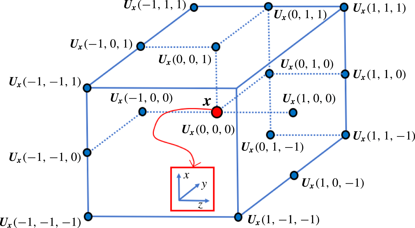
Second, we define $\boldsymbol{U}_{\boldsymbol{x}}=\boldsymbol{U}_{\boldsymbol{x},\left(0,0,0\right)}\in \mathbb{R}^{n}$ to be the displacement vector at pixel position $\boldsymbol{x}$ , and $\boldsymbol{U}_{\boldsymbol{x},N_{R}}$ is the set of its $[\left(2R+1\right)^{3}-1]$ neighbours. Figure 2 illustrates the neighbourhood for $R=1$ . Additionally, let $\boldsymbol{U}_{\boldsymbol{x},med}$ be the median of $\boldsymbol{U}_{\boldsymbol{x},N_{R}}$ . The classical median test value is defined as $\left(\text{MT}\right)_{\boldsymbol{x},N_{R}}=\Vert \boldsymbol{U}_{\boldsymbol{x},med}-\boldsymbol{U}_{\boldsymbol{x}}\Vert$ , which is passed if it is smaller than a user-defined threshold value $\unicode[STIX]{x1D716}_{t}$ . Furthermore, we define the set of residuals, $r_{\boldsymbol{x},N_{R}}$ , as

(3.2) $$\begin{eqnarray}r_{\boldsymbol{x},N_{R}}=\{r\in \mathbb{R}\mid r=\Vert \boldsymbol{U}-\boldsymbol{U}_{\boldsymbol{x},med}\Vert \wedge \boldsymbol{U}\in \boldsymbol{U}_{\boldsymbol{x},N_{R}}\},\end{eqnarray}$$

and, similarly, $r_{\boldsymbol{x},med}$ is defined to be the median of $r_{\boldsymbol{x},N_{R}}$ , which is used to normalise the usual median test,

(3.3) $$\begin{eqnarray}\left(\text{NMT}\right)_{\boldsymbol{x},N_{R}}=\frac{\Vert \boldsymbol{U}_{\boldsymbol{x},med}-\boldsymbol{U}_{\boldsymbol{x}}\Vert }{r_{\boldsymbol{x},med}+\unicode[STIX]{x1D716}}<\unicode[STIX]{x1D716}_{t}.\end{eqnarray}$$

Figure 2.

For $R=1$ , the set $\boldsymbol{U}_{\boldsymbol{x},N_{1}}$ is shown with the $26$ neighbours of $\boldsymbol{U}_{\boldsymbol{x}}$ (not all neighbours illustrated). It should be noted that $N_{R}$ does not contain the tuple $(0,0,0)$ ; hence, $\boldsymbol{U}_{\boldsymbol{x}}=\boldsymbol{U}_{\boldsymbol{x},(0,0,0)}$ is not included in $\boldsymbol{U}_{\boldsymbol{x},N_{1}}$ .

Under uniform flow conditions, the main normalisation factor $r_{\boldsymbol{x},med}$ tends to yield zero; hence, a small and acceptable local fluctuation level $\unicode[STIX]{x1D716}$ is applied to compensate for a potential division by zero and to account for remaining velocity fluctuations obtained from cross-correlation analysis. In practice, $\unicode[STIX]{x1D716}$ values between $0.1$ and $0.2$ might be used (Westerweel & Scarano Reference Westerweel and Scarano2005; Raffel et al. Reference Raffel, Willert, Wereley and Kompenhans2007; Garcia Reference Garcia2011). In our case, $\unicode[STIX]{x1D716}=0.2$ performed well for the available MR flow data. Furthermore, $\unicode[STIX]{x1D716}_{t}=2.25$ is used as the validation threshold. Once the latter parameter is detected from numerical experiments, it can be used for other data in similar flow regimes with the same imaging modality.

Prior to the application of noise detection, the observations $\boldsymbol{u}_{\boldsymbol{m}\boldsymbol{r}\boldsymbol{i}}$ obtained from MRI measurements are initially already divergence-free. This is ensured by the constraints applied during the reconstruction process of the MRI data, which is out of the scope of this work. After denoising, however, the detected spurious vectors are erased from the data, which results in a flow field $\boldsymbol{u}_{\boldsymbol{m}\boldsymbol{r}\boldsymbol{i}}^{\circ }$ with gaps at certain positions within the observations. This clearly violates the divergence-free property of the observed data $\boldsymbol{u}_{\boldsymbol{m}\boldsymbol{r}\boldsymbol{i}}$ . One possible way to fill in the gaps would be the use of some interpolation scheme. However, such schemes will not necessarily ensure a solenoidal flow field. Therefore, we rely on the application of a projection over a divergence-free space at a later stage (see § 3.4) to automatically fill in the aforementioned gaps and to recover back the divergence-free property of the flow field.

3.2 Segmentation and registration

After the removal of outliers, the arterial structures, in which the analysis is to be performed, are segmented from both the artificially generated flow data as well as the acquired MR measurements. The experimental MRI data comprise the anatomical structures and the velocity field data (Markl et al. Reference Markl, Frydrychowicz, Kozerke, Hope and Wieben2012), whereas the artificial flow data consist of the flow field generated either in a cylindrical geometry or in the geometry of the phantom aorta. For validation studies in the simplified domain, the flow data were used for segmentation of the cylindrical geometry (see § 4), whereas for experimental and complementary validation studies, the anatomical data from MR images were used to extract the vascular geometry from the aorta replica (see § 5). The segmentation was performed using the snake evolution method available in ITK-SNAP (http://www.itksnap.org) and was smoothed using the tools available in the VMTK library (http://www.vmtk.org). This procedure is expected to suffer from the low resolution and partial volume effects of flow MRI data.

For the comparison with experimental MRI data, high-resolution aortic surface data were already available from the $3$ -D print of the glass replica. The latter were used to generate the computational mesh for the exact geometry. However, after image acquisition and segmentation, the flow data are misaligned with the exact geometry of the replica. Therefore, a registration step was necessary to align the measured flow field with the exact geometry of the replica. The rigid registration was performed using the iterative closest point (ICP) algorithm, which aims to minimise the distance between two sets of points. The numbers of available points in the point clouds of both the exact and the segmented geometries were approximately 1600 000 and 12 000 respectively. Prior to the registration process, 5000 points were randomly sampled from each geometry, which were then used as the two point input clouds for the ICP algorithm. The root-mean-square error between the registered point clouds was 0.001. In the case of the artificially generated flow data in the cylindrical domain, no registration step was required, since the geometry was already aligned with the segmented domain.

3.3 Mapping in the computational mesh

For both cases, the analytical geometry (cylinder) and the experimental geometry (glass replica of aorta), the available exact geometries were used to generate the computational mesh domain, which was used for the flow simulations. For both datasets, a hexahedral mesh was created using OpenFOAM’s snappyHexMesh procedure. In the case of the experimental geometry, the mesh was rigidly transformed into its corresponding segmentation using the mapping obtained from the registration step. After mesh generation, the velocities, $\boldsymbol{u}_{\boldsymbol{m}\boldsymbol{r}\boldsymbol{i}}^{\circ }$ , from the denoised phase difference images (obtained from $4$ -D flow MRI and denoised with the universal outlier detection scheme) with limited resolution (i.e. in a coarse observational domain) were mapped into the fine hexahedral mesh (computational domain for CFD simulations with high resolution) using the linear interpolation method available in ITK (Johnson et al. Reference Johnson, Mccormick and Ibáñez2013). As a result of the combination of the linear interpolation and the previous noise detection process, the final flow field (denoted by $\bar{\boldsymbol{u}}_{\boldsymbol{m}\boldsymbol{r}\boldsymbol{i}}$ ) in the CFD mesh was not divergence-free. The divergence-free property was then recovered with the projection over a divergence-free space applied to the velocity field in the CFD mesh, as explained next.

3.4 Projection into divergence-free space

Let $\bar{\boldsymbol{u}}_{\boldsymbol{m}\boldsymbol{r}\boldsymbol{i}}\in (L^{2}(\unicode[STIX]{x1D6FA}))^{3}$ be a given observation, projected into a bounded Lipschitz domain $\unicode[STIX]{x1D6FA}\in \mathbb{R}^{3}$ with boundary $\unicode[STIX]{x2202}\unicode[STIX]{x1D6FA}$ . According to Helmholtz–Hodge decomposition (HHD), the velocity field can be decomposed into the sum of its divergence-free, curl-free and gradient of harmonic components, if the velocity is known at the boundary (Denaro Reference Denaro2003; Harouna & Perrier Reference Harouna, Perrier, Boissonnat, Chenin, Cohen, Gout, Lyche, Mazure and Schumaker2012; Bhatia et al. Reference Bhatia, Norgard, Pascucci and Bremer2013). In this work, we reconstruct the divergence-free flow field by removing the gradient of the harmonic component and solving the following problem:

(3.4) $$\begin{eqnarray}\left.\begin{array}{@{}c@{}}\mathscr{P}_{\bot }(\bar{\boldsymbol{u}}_{\boldsymbol{m}\boldsymbol{r}\boldsymbol{i}})\boldsymbol{ : }\text{ given }\bar{\boldsymbol{u}}_{\boldsymbol{m}\boldsymbol{r}\boldsymbol{i}},\text{ find }\tilde{\boldsymbol{u}}^{\star }=\bar{\boldsymbol{u}}_{\boldsymbol{m}\boldsymbol{r}\boldsymbol{i}}-\unicode[STIX]{x1D735}q\text{ such that}\\ \unicode[STIX]{x0394}q=\unicode[STIX]{x1D735}\boldsymbol{\cdot }\bar{\boldsymbol{u}}_{\boldsymbol{m}\boldsymbol{r}\boldsymbol{i}}\text{ in }\unicode[STIX]{x1D6FA}\\ q=0\text{ on }\unicode[STIX]{x1D6E4}_{w}\quad \text{ and }\quad \unicode[STIX]{x1D735}q\boldsymbol{\cdot }\boldsymbol{n}=0\text{ on }\unicode[STIX]{x2202}\unicode[STIX]{x1D6FA}\backslash \unicode[STIX]{x1D6E4}_{w}.\end{array}\right\}\end{eqnarray}$$

The problem $\mathscr{P}_{\bot }$ differs from the HHD in terms of the applied BCs, but under certain modifications the HHD can be recovered. Although the problem $\mathscr{P}_{\bot }$ does not directly correspond to the HHD, it still represents a projection over a space of divergence-free flow fields.

The observations, $\bar{\boldsymbol{u}}_{\boldsymbol{m}\boldsymbol{r}\boldsymbol{i}}$ , are assumed to be already modified by the application of the universal outlier detection scheme (as described in § 3.1) prior to its projection in the CFD mesh. The projection ( $\boldsymbol{u}_{\boldsymbol{m}\boldsymbol{r}\boldsymbol{i}}^{\circ }\rightarrow \bar{\boldsymbol{u}}_{\boldsymbol{m}\boldsymbol{r}\boldsymbol{i}}$ ) is performed by linear interpolation. Problem $\mathscr{P}_{\bot }$ is solved using OpenFOAM’s (Weller et al. 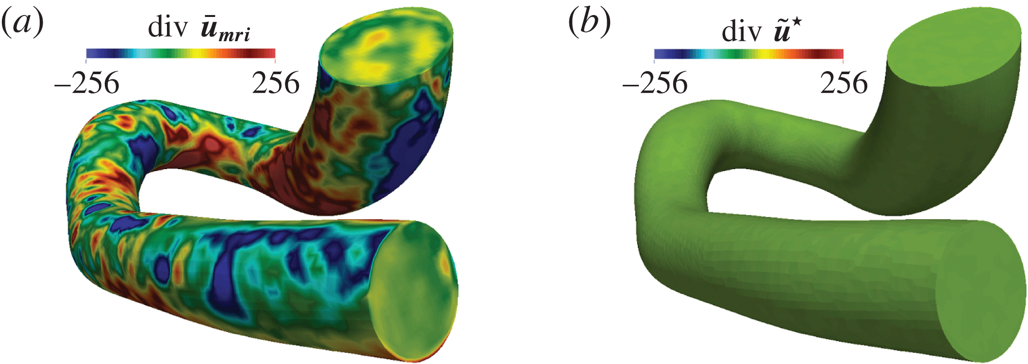Reference Weller, Tabor, Jasak and Fureby1998) conjugate gradient solver (PCG) with simplified diagonal-based incomplete Cholesky preconditioner (DIC). Figure 3 illustrates that the projection into the space of divergence-free vector fields (in the phantom replica of the human aorta) recovers the divergence-free property of the flow field to a great extent.

Figure 3.

The divergence of the flow field in a phantom of a human aorta acquired with MRI: (a) raw data, before the application of the divergence-free projection operator, $\mathscr{P}_{\bot }$ ; (b) the divergence-free flow field, after the application of $\mathscr{P}_{\bot }$ .

4.1 Poiseuille flow

We consider the fully developed laminar flow of a Newtonian fluid in a cylinder of length $L$ , constant cross-sectional area $A$ and diameter $D$ ( $R=D/2$ is the pipe radius). The solution of the Navier–Stokes equations in this case yields

(4.1) $$\begin{eqnarray}\boldsymbol{u}_{\boldsymbol{e}\boldsymbol{x}\boldsymbol{t}}(r)=\frac{\unicode[STIX]{x0394}PD^{2}}{16\unicode[STIX]{x1D708}\unicode[STIX]{x1D70C}L}\left(1-\frac{r^{2}}{R^{2}}\right).\end{eqnarray}$$

From (4.1), and calling $\boldsymbol{U}_{\boldsymbol{a}\boldsymbol{v}\boldsymbol{r}}$ the average velocity, it can be derived that $\boldsymbol{u}_{\boldsymbol{e}\boldsymbol{x}\boldsymbol{t}}(r)=2\boldsymbol{U}_{\boldsymbol{a}\boldsymbol{v}\boldsymbol{r}}(1-r^{2}/R^{2})$ . Finally, taking $Re=D\boldsymbol{U}_{\boldsymbol{a}\boldsymbol{v}\boldsymbol{r}}/\unicode[STIX]{x1D708}$ , the analytical solution can be given in terms of the Reynolds number and kinematic viscosity as

(4.2) $$\begin{eqnarray}\boldsymbol{u}_{\boldsymbol{e}\boldsymbol{x}\boldsymbol{t}}(r)=\frac{2\unicode[STIX]{x1D708}Re}{D}\left(1-\frac{r^{2}}{R^{2}}\right).\end{eqnarray}$$

4.2 Evaluation of analytical solution

During the MRI acquisition process, the velocities are spatially averaged. To simulate such a framework, the exact solution from (4.2) needs to be spatially averaged to the desired MRI voxel size. Since it is not possible to calculate the exact solution for an infinite number of points, its evaluation was performed on each cell centre of a fine hexahedral mesh with $3693\,600$ cells. 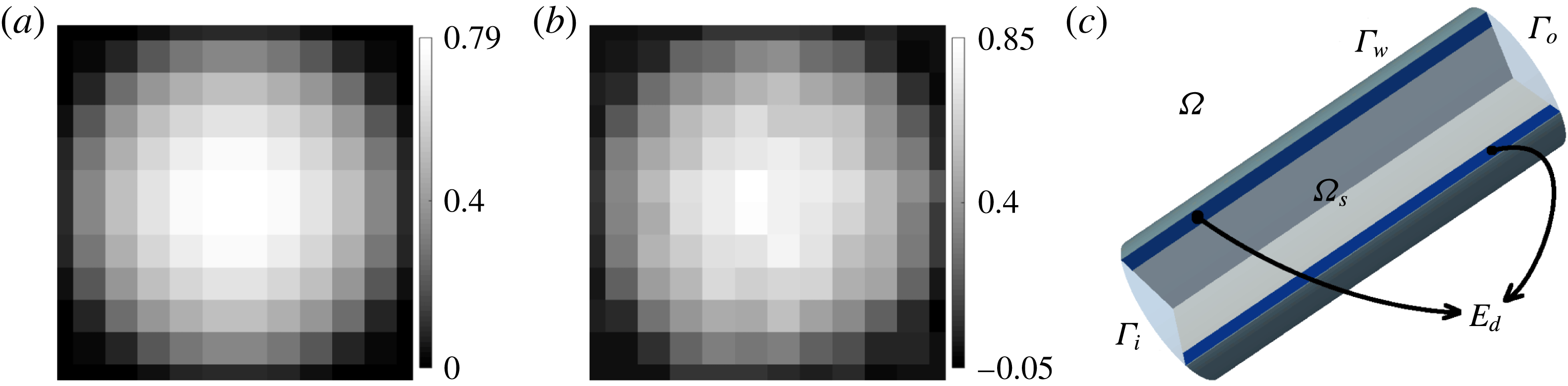The cylinder radius was $R=1.2$ cm (diameter $D=2.4$ cm) and the length was $L=6$ cm (see figure 4 c). As the solution described by the Hagen–Poiseuille equation (4.1) is valid for laminar flow, the Reynolds number was chosen to be $2000$ . Finally, as a reasonable approximation of blood viscosity in the human aorta, the kinematic viscosity was chosen to be $\unicode[STIX]{x1D708}=4.8$ cP. Under these conditions, the maximum flow velocity in the aforementioned cylinder approximately results in $|\boldsymbol{u}|_{max}\approx 0.8~\text{m}~\text{s}^{-1}$ .

Figure 4.

Artificially generated velocity images ( $2$ mm isotropic voxel size) of both (a) the exact solution and (b) the integrated noise with an SNR of 20, before their mapping into (c) the computational flow domain.

4.3 Generation of artificial MRI data

The acquired velocities with flow MRI are proportional to the phase shift in the signal of spins moving along a magnetic gradient field. Since the phase of a signal is limited to $2\unicode[STIX]{x03C0}$ radians, so is also the range of velocities that can be detected uniquely. The highest velocity that is likely to be encountered within the region of interest is held within a user-defined velocity encoding (VENC). For velocity magnitudes higher than the VENC, the so-called velocity aliasing effect (or phase wrap-around artefact) occurs, which prevents the unique assignment of the velocities. The quality of flow MRI suffers from velocity noise, which is proportional to the velocity encoding and inversely associated with the signal-to-noise ratio (SNR) in the related phase difference images (Pelc et al. Reference Pelc, Herfkens, Shimakawa and Enzmann1991). As described by Pelc et al. (Reference Pelc, Herfkens, Shimakawa and Enzmann1991), the standard deviation of the velocity can be approximated as

(4.3) $$\begin{eqnarray}\unicode[STIX]{x1D70E}_{u}\approx (0.45\ast \text{VENC})/\text{SNR}.\end{eqnarray}$$

Gudbjartsson & Patz (Reference Gudbjartsson and Patz1995) showed that in the existence of noise, the image intensity in phase-contrast MRI is governed by the Rician distribution. For SNR greater than two, the noise distribution is shown to be nearly Gaussian. The analytical solution evaluated in the fine mesh was first averaged into an MRI grid of $2$  mm voxel size in each direction, as shown in figure 4(a). Gaussian white noise was added thereafter on the averaged velocities, as shown in figure 4(b). The VENC was chosen to be $120~\text{cm}~\text{s}^{-1}$ in the longitudinal direction ( $z$ ), whereas it was $20~\text{cm}~\text{s}^{-1}$ in the remaining directions ( $x$ and $y$ ). The standard deviation of the velocity was chosen such that the noise amplitude corresponded to an SNR of $20$ . As the cylinder is user-defined, the acquired flow field is already registered with the exact geometry. After the addition of artificial noise, the thus-simulated MRI data follow the preprocessing pipeline (with the exception of the registration stage), as described in § 3, before starting the CFD simulation. In what follows, $\boldsymbol{u}_{\boldsymbol{s}\boldsymbol{n}\boldsymbol{r}}$ will represent the noisy MRI measurements, which are mapped into the computational domain and for which a decomposition is applied to project the field over a divergence-free space, as described in §§ 3.3 and 3.4. The cylindrical computational domain is illustrated in figure 4(c).

4.4 Optimisation with exact solution as target flow

First, we consider one case where the optimisation starts with a noisy flow field and is performed against the exact solution. That is, the target flow field $\tilde{\boldsymbol{u}}^{t}$ in the objective function (2.5) corresponds to $\boldsymbol{u}_{\boldsymbol{e}\boldsymbol{x}\boldsymbol{t}}$ given by (4.2). In addition, the initial condition, $(\boldsymbol{u})_{0}=\boldsymbol{u}^{0}$ , corresponds to the artificially generated divergence-free flow field, $\boldsymbol{u}_{\boldsymbol{s}\boldsymbol{n}\boldsymbol{r}}$ , as described in § 4.3. Thus, algorithm 1 is executed with the input parameters $(\boldsymbol{u}_{\boldsymbol{s}\boldsymbol{n}\boldsymbol{r}},\boldsymbol{g}_{\boldsymbol{s}\boldsymbol{n}\boldsymbol{r}},\boldsymbol{u}_{\boldsymbol{e}\boldsymbol{x}\boldsymbol{t}})$ , where $\boldsymbol{g}_{\boldsymbol{s}\boldsymbol{n}\boldsymbol{r}}=\boldsymbol{u}_{\boldsymbol{s}\boldsymbol{n}\boldsymbol{r}}$ on $\unicode[STIX]{x1D6E4}_{i}$ . In what follows, we will denote $\boldsymbol{u}_{\boldsymbol{o}\boldsymbol{p}\boldsymbol{t}}=\boldsymbol{u}_{\boldsymbol{o}\boldsymbol{p}\boldsymbol{t}}^{k}$ as the solution returned by the optimisation process after $k$ iterations of algorithm 1. The mesh is set up with $118\,800$ cells including $114\,840$ hexahedras and $3960$ prisms. The size of the mesh is suitable to obtain satisfactory results. Flow-matching domains, $\unicode[STIX]{x1D6FA}_{s}$ , $\unicode[STIX]{x1D6E4}_{si}$ and $\unicode[STIX]{x1D6E4}_{so}$ (see figure 4 c), cover the lumen, including both inlet and outlet boundaries. In what follows, we will give a meaning to the subscript, $s$ , in the flow-matching domain, $\unicode[STIX]{x1D6FA}_{s}$ . The subscript $s$ prescribes the extent of contraction of the whole domain $\unicode[STIX]{x1D6FA}$ in millimetres (mm), as follows:

(4.4) $$\begin{eqnarray}\unicode[STIX]{x1D6FA}_{s}=\{\boldsymbol{x}\in \unicode[STIX]{x1D6FA}\mid \Vert \boldsymbol{x}-\boldsymbol{y}\Vert \geqslant s(\text{mm})\,\forall \boldsymbol{y}\in \unicode[STIX]{x1D6E4}_{w}\}.\end{eqnarray}$$

In this set-up, we set $s=2$ . That is, the flow-matching domain $\unicode[STIX]{x1D6FA}_{s}$ is a contracted domain of $\unicode[STIX]{x1D6FA}$ such that the distance to $\unicode[STIX]{x1D6E4}_{w}$ is at least $2$ mm. Figure 4(c) shows the example of $\unicode[STIX]{x1D6FA}_{s}$ in the cylinder. Furthermore, the optimisation parameters are $\unicode[STIX]{x1D6FC}=0.15$ , $\unicode[STIX]{x1D6FD}=10^{-4}$ and $\unicode[STIX]{x1D6FD}_{1}=10^{-8}$ . 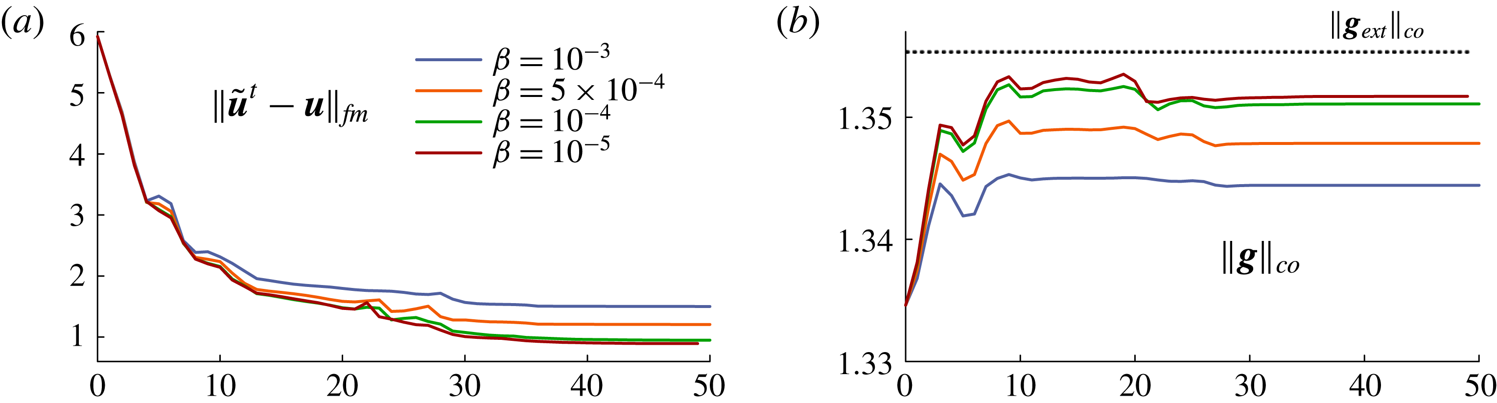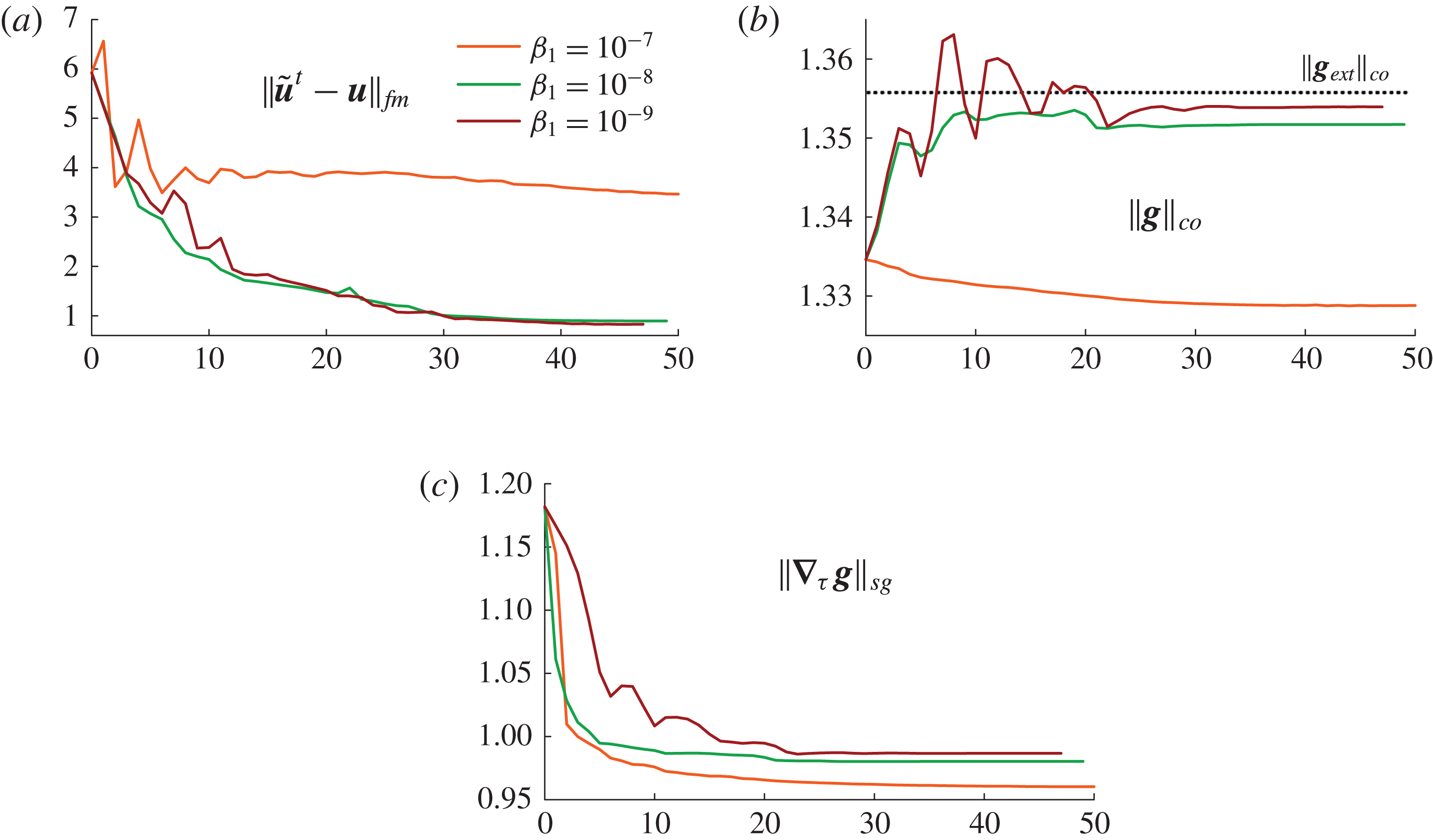Figure 5(a–c) illustrates the norms of the flow matching, $\Vert \tilde{\boldsymbol{u}}^{t}-\boldsymbol{u}\Vert _{fm}$ , the control, $\Vert \boldsymbol{g}\Vert _{co}$ , and the surface gradient of the control, $\Vert \unicode[STIX]{x1D735}_{\unicode[STIX]{x1D749}}~\boldsymbol{g}\Vert _{sg}$ , which are defined as follows:

(4.5) $$\begin{eqnarray}\displaystyle & \displaystyle \Vert \tilde{\boldsymbol{u}}^{t}-\boldsymbol{u}\Vert _{fm}=\left(\frac{100}{\underset{\unicode[STIX]{x1D6FA}}{\text{avr}}|\tilde{\boldsymbol{u}}^{t}|}\right)\sqrt{\frac{1}{V_{\unicode[STIX]{x1D6FA}}}\int _{\unicode[STIX]{x1D6FA}}|\tilde{\boldsymbol{u}}^{t}-\boldsymbol{u}|^{2}\,\text{d}\unicode[STIX]{x1D6FA}}, & \displaystyle\end{eqnarray}$$

(4.6) $$\begin{eqnarray}\displaystyle & \displaystyle \Vert \boldsymbol{g}\Vert _{co}=\left(\frac{1}{\underset{\unicode[STIX]{x1D6E4}_{i}}{\text{avr}}|\tilde{\boldsymbol{u}}^{t}|}\right)\sqrt{\frac{1}{A_{\unicode[STIX]{x1D6E4}_{i}}}\int _{\unicode[STIX]{x1D6E4}_{i}}|\boldsymbol{g}|^{2}\,\text{d}\unicode[STIX]{x1D6E4}}, & \displaystyle\end{eqnarray}$$

(4.7) $$\begin{eqnarray}\displaystyle & \displaystyle \Vert \unicode[STIX]{x1D735}_{\unicode[STIX]{x1D749}}~\boldsymbol{g}\Vert _{sg}=\left(\frac{1}{\underset{\unicode[STIX]{x1D6E4}_{i}}{\text{avr}}|\unicode[STIX]{x1D735}_{\unicode[STIX]{x1D749}}\tilde{\boldsymbol{u}}^{t}|}\right)\sqrt{\frac{1}{A_{\unicode[STIX]{x1D6E4}_{i}}}\int _{\unicode[STIX]{x1D6E4}_{i}}|\unicode[STIX]{x1D735}_{\unicode[STIX]{x1D749}}\boldsymbol{g}|^{2}\,\text{d}\unicode[STIX]{x1D6E4}}, & \displaystyle\end{eqnarray}$$

where $V_{\unicode[STIX]{x1D6FA}}$ is the volume of the entire domain and $A_{\unicode[STIX]{x1D6E4}_{i}}$ is the area at the inlet. The norms are normalised against the average magnitude of the target velocity or its surface gradient.

Figure 5.

The norms from optimisation with parameters $\unicode[STIX]{x1D6FC}=0.15$ , $\unicode[STIX]{x1D6FD}=10^{-4}$ and $\unicode[STIX]{x1D6FD}_{1}=10^{-8}$ . The norms are plotted against the number of iterations on the horizontal axis. (a) Flow matching, (b) control, (c) surface gradient of control.

As can be seen in figure 5(b), the norm of the control, $\Vert \boldsymbol{g}\Vert _{co}$ , rapidly grows at the beginning, forcing the noisy vectors towards their desired position and remaining almost constant after a while. In figure 5(c), the sudden decrease in the norm of the velocity surface gradient, $\Vert \unicode[STIX]{x1D735}_{\unicode[STIX]{x1D749}}~\boldsymbol{g}\Vert _{sg}$ , shows the denoising process at the inlet. Once a good approximation is reached, the velocities at the inlet are only being adjusted slightly during the rest of the iterations. This is continued until a sufficient flow matching is achieved in the entire domain, as illustrated in figure 5(a).

Let us now focus on the results in the domain close to the cylinder wall. To confirm the presented results also with respect to the accuracy in the near-wall regions, we calculated both the root-mean-square error, $\text{nRMSE}_{d}=\text{nRMSE}_{d}(\boldsymbol{u}_{\boldsymbol{e}\boldsymbol{x}\boldsymbol{t}},\boldsymbol{u}_{\boldsymbol{o}\boldsymbol{p}\boldsymbol{t}})$ , and the flow direction error, $\text{FDE}_{d}=\text{FDE}_{d}(\boldsymbol{u}_{\boldsymbol{e}\boldsymbol{x}\boldsymbol{t}},\boldsymbol{u}_{\boldsymbol{o}\boldsymbol{p}\boldsymbol{t}})$ , defined by

(4.8) $$\begin{eqnarray}\displaystyle & \displaystyle \text{nRMSE}_{d}(\boldsymbol{u}_{t},\boldsymbol{u}_{c})=\left(\frac{100}{\underset{E_{d}}{\text{avr}}|\boldsymbol{u}_{t}|}\right)\sqrt{\frac{1}{V_{d}}\int _{E_{d}}|\boldsymbol{u}_{t}-\boldsymbol{u}_{c}|^{2}\,\text{d}E_{d}}, & \displaystyle\end{eqnarray}$$

(4.9) $$\begin{eqnarray}\displaystyle & \displaystyle \text{FDE}_{d}(\boldsymbol{u}_{t},\boldsymbol{u}_{c})=\sqrt{\frac{1}{V_{d}}\int _{E_{d}}\left(1-\frac{\boldsymbol{u}_{t}\boldsymbol{\cdot }\boldsymbol{u}_{c}}{|\boldsymbol{u}_{t}||\boldsymbol{u}_{c}|}\right)^{2}\,\text{d}E_{d}}. & \displaystyle\end{eqnarray}$$

In what follows, the subscript $d$ stands for the evaluation of the error within the contracted subdomain $E_{d}\subset \unicode[STIX]{x1D6FA}$ with volume $V_{d}$ , which is defined as

(4.10) $$\begin{eqnarray}E_{d}=\{\boldsymbol{x}\in \unicode[STIX]{x1D6FA}\mid \exists \boldsymbol{y}\in \unicode[STIX]{x1D6E4}_{w},\Vert \boldsymbol{x}-\boldsymbol{y}\Vert <d\text{ (mm)}\}.\end{eqnarray}$$

That is, we want to evaluate the errors in the domain $E_{d}$ at near-wall regions (this domain is not meant to be included in the flow-matching domain $\unicode[STIX]{x1D6FA}_{s}$ ), where the nearest Euclidean distance of all points in $E_{d}$ is at most $d$ mm apart from the wall, $\unicode[STIX]{x1D6E4}_{w}$ . Figure 4(c) features the contracted domain in the cylinder. It should be noted that both errors, (4.8) and (4.9), are evaluated between the exact solution, $\boldsymbol{u}_{\boldsymbol{e}\boldsymbol{x}\boldsymbol{t}}$ , and the results obtained from the proposed optimisation strategy, $\boldsymbol{u}_{\boldsymbol{o}\boldsymbol{p}\boldsymbol{t}}$ , in the contracted region $E_{d}$ . In addition, the error $\text{nRMSE}_{d}$ is normalised against the average velocity magnitude of the observations in $E_{d}$ .

For $d=2$ , the initial errors $\text{nRMSE}_{2}(\boldsymbol{u}_{\boldsymbol{e}\boldsymbol{x}\boldsymbol{t}},\boldsymbol{u}_{\boldsymbol{s}\boldsymbol{n}\boldsymbol{r}})$ and $\text{FDE}_{2}(\boldsymbol{u}_{\boldsymbol{e}\boldsymbol{x}\boldsymbol{t}},\boldsymbol{u}_{\boldsymbol{s}\boldsymbol{n}\boldsymbol{r}})$ between the exact solution, $\boldsymbol{u}_{\boldsymbol{e}\boldsymbol{x}\boldsymbol{t}}$ , and noisy observations, $\boldsymbol{u}_{\boldsymbol{s}\boldsymbol{n}\boldsymbol{r}}$ , were $26.65\,\%$ and $1.1\times 10^{-2}$ respectively. After optimal control, the root-mean-square error, as a percentage of the average velocity magnitude, was reduced to $\text{nRMSE}_{2}(\boldsymbol{u}_{\boldsymbol{e}\boldsymbol{x}\boldsymbol{t}},\boldsymbol{u}_{\boldsymbol{o}\boldsymbol{p}\boldsymbol{t}})=3.53\,\%$ , and the flow direction error was $\text{FDE}_{2}(\boldsymbol{u}_{\boldsymbol{e}\boldsymbol{x}\boldsymbol{t}},\boldsymbol{u}_{\boldsymbol{o}\boldsymbol{p}\boldsymbol{t}})=3.5\times 10^{-5}$ .

4.4.1 Sensitivity analyses with respect to changes in optimisation parameters

There have been some reported discussions in the literature concerning the choice of the optimisation parameters for related control problems, mostly based on simplified 2-D geometries. In Lee (Reference Lee2011), the penalisation value was set to $10^{-10}$ for a Neumann boundary control and validations were performed for a flow problem in a 2-D square case. In Guerra, Tiago & Sequeira (Reference Guerra, Tiago and Sequeira2014), a 2-D geometry for a stenosed vessel was considered, where the parameter related to the surface gradient term (denoted as $\unicode[STIX]{x1D6FD}_{1}$ in this work) was set to $10^{x}$ , with $x\in \{-5,-4,-2,-1,0,1\}$ , whereas the other optimisation parameters were maintained constant. Further works have also reported on the choice of regularisation parameters in the related field (Fursikov, Gunzburger & Hou Reference Fursikov, Gunzburger and Hou1998; D’Elia et al. Reference D’Elia, Mirabella, Passerini, Perego, Piccinelli, Vergara, Veneziani, Ambrosi, Quarteroni and Rozza2012a ; Bertagna et al. Reference Bertagna, D’Elia, Perego, Veneziani, Bodnár, Galdi and Nečasová2014; Guerra et al. Reference Guerra, Sequeira and Tiago2015).

In this work, the parameter $\unicode[STIX]{x1D6FC}$ was chosen on a trial and error basis. It was observed that $\unicode[STIX]{x1D6FC}$ should be between 0.15 and 0.5 depending on the data being used. Values larger than 0.5 enforce a more stringent flow matching, and the optimiser already stops at very early stages of the iterations. For values smaller than 0.15, the optimiser performs more iterations because the flow-matching term is more relaxed. In the latter case, as expected, the final solution gets further away from the observations.

The differences in the response as a consequence of changes in the optimisation parameters, $\unicode[STIX]{x1D6FD}$ and $\unicode[STIX]{x1D6FD}_{1}$ , were examined in this work for the 3D case. First of all, we set $\unicode[STIX]{x1D6FC}=0.15$ , which was experimentally found to be an appropriate parameter for this use case and was then used in the sensitivity analyses with respect to changes in $\unicode[STIX]{x1D6FD}$ and $\unicode[STIX]{x1D6FD}_{1}$ . Second, we kept $\unicode[STIX]{x1D6FD}_{1}=10^{-8}$ fixed and modified $\unicode[STIX]{x1D6FD}$ . Figure 6(a,b) shows the flow-matching norm, $\Vert \tilde{\boldsymbol{u}}^{t}-\boldsymbol{u}\Vert _{fm}$ , and the control norm, $\Vert \boldsymbol{g}\Vert _{co}$ , for different $\unicode[STIX]{x1D6FD}$ values. In addition, figure 6(b) also contains the constant norm, $\Vert \boldsymbol{g}_{\boldsymbol{e}\boldsymbol{x}\boldsymbol{t}}\Vert _{co}$ , of the exact solution. We observed that for larger values, such as $\unicode[STIX]{x1D6FD}>10^{-4}$ , there was not enough control and the flow matching was poor. This is because the objective function was rapidly penalised at early stages of the optimisation, where the optimiser needs larger controls in order to reduce the error. For smaller $\unicode[STIX]{x1D6FD}$ values, however, there was no hard penalisation and the optimiser could apply larger controls, as illustrated in figure 6(b). In general, the values $10^{-4}$ and $10^{-5}$ delivered satisfactory results, and $\unicode[STIX]{x1D6FD}=10^{-5}$ was observed to be the best choice. Furthermore, we fixed $\unicode[STIX]{x1D6FD}$ at $10^{-5}$ and ran the optimiser with $\unicode[STIX]{x1D6FD}_{1}$ set to $10^{-7}$ , $10^{-8}$ and $10^{-9}$ (smaller values of $\unicode[STIX]{x1D6FD}_{1}$ rendered unacceptable solutions because of the lack of smoothing effect on noisy measurements). For different $\unicode[STIX]{x1D6FD}_{1}$ values, figure 7(a,c) shows the plots for the flow-matching norm, $\Vert \tilde{\boldsymbol{u}}^{t}-\boldsymbol{u}\Vert _{fm}$ , and the surface gradient norm, $\Vert \unicode[STIX]{x1D735}_{\unicode[STIX]{x1D749}}~\boldsymbol{g}\Vert _{sg}$ . Let us first analyse the results between the values $10^{-7}$ and $10^{-8}$ for $\unicode[STIX]{x1D6FD}_{1}$ . It can be observed that the norm of the surface gradient is further reduced for $\unicode[STIX]{x1D6FD}_{1}=10^{-8}$ over the successive iterations, and better flow matching is achieved. This can be explained by further investigation of the control norm, $\Vert \boldsymbol{g}\Vert _{co}$ , along with the norm of the exact solution, $\Vert \boldsymbol{g}_{\boldsymbol{e}\boldsymbol{x}\boldsymbol{t}}\Vert _{co}$ , in figure 7(b). We can observe that there is not enough control for $\unicode[STIX]{x1D6FD}_{1}=10^{-7}$ . This shows that even if we are able to remove the noise at the inlet (which is explained by the reduction in the value of the surface gradient for $\unicode[STIX]{x1D6FD}_{1}=10^{-7}$ ), the controls are small and hence the velocities cannot be properly controlled. Second, let us consider the results for $\unicode[STIX]{x1D6FD}_{1}$ values of $10^{-8}$ and $10^{-9}$ . Figure 7(a) shows that the flow matching is achieved with an almost equally good quality. In figure 7(b), however, fluctuations along the iterations can be observed in the norm of controls for $\unicode[STIX]{x1D6FD}_{1}=10^{-9}$ . In addition, figure 7(c) shows that the fluctuations also have an effect on the norm of the surface gradient, which is not as greatly reduced in early iterations as is the case for $\unicode[STIX]{x1D6FD}_{1}=10^{-8}$ . Finally, our interpretations are also confirmed quantitatively in near-wall regions. Table 1 summarises the results from the sensitivity analysis comparing the root-mean-square errors, $\text{nRMSE}_{2}$ , and the flow direction errors, $\text{FDE}_{2}$ , for varied optimisation parameters. Our conclusion is that a value of $\unicode[STIX]{x1D6FD}_{1}=10^{-8}$ delivers sufficiently accurate results, and this value will be used hereafter.

Table 1.

Dimensionless root-mean-square ( $\text{nRMSE}_{2}(\boldsymbol{u}_{\boldsymbol{e}\boldsymbol{x}\boldsymbol{t}},\boldsymbol{u}_{\boldsymbol{o}\boldsymbol{p}\boldsymbol{t}})$ ) and flow direction ( $\text{FDE}_{2}(\boldsymbol{u}_{\boldsymbol{e}\boldsymbol{x}\boldsymbol{t}},\boldsymbol{u}_{\boldsymbol{o}\boldsymbol{p}\boldsymbol{t}})$ ) errors measured within the near-wall ( $2$ mm) domain ( $E_{2}$ ).

Figure 6.

Alteration in norms of (a) flow matching and (b) control (solid lines in a,b) with respect to changes in $\unicode[STIX]{x1D6FD}$ , along with the constant norm of the exact solution (dashed line in b), where $\unicode[STIX]{x1D6FC}=0.15$ and $\unicode[STIX]{x1D6FD}_{1}=10^{-8}$ . The norms are plotted against the number of iterations on the horizontal axis.

Figure 7.

Alteration in norms of (a) flow matching, (b) control and (c) control surface gradient (solid lines in a–c) with respect to changes in $\unicode[STIX]{x1D6FD}_{1}$ , along with the constant norm of the exact solution (dashed line in b), where $\unicode[STIX]{x1D6FC}=0.15$ and $\unicode[STIX]{x1D6FD}=10^{-5}$ . The norms are plotted against the number of iterations on the horizontal axis.

4.5 Optimisation with noisy solution as target flow

So far, we have been able to validate the proposed approach using an analytical solution. Actually, an exact solution is not available or cannot be provided by measurements or experiments. Here, the performance of the optimisation framework was evaluated considering the artificially generated noisy measurements as the target flow. That is, we set $\tilde{\boldsymbol{u}}^{t}=\boldsymbol{u}_{\boldsymbol{s}\boldsymbol{n}\boldsymbol{r}}$ in the objective function (2.5). In order to avoid lack of control, the initial flow field was low-pass filtered with a cutoff frequency of $0.5$ . The low-pass filtered field is just a smoothed version of the measurements. It reduces the edge contents and results in a blurred image. The degree of the smoothness is proportional to the chosen cutoff frequency. Use of a blurred (smoothed or low-pass filtered) version of the measurements as initial condition is not mandatory. However, the motivation behind using it was the fact that, preferably, the flow-matching term in the objective function (first term in (2.5)) should not result in a null value at the very first iteration (e.g. by the application of the measurements directly as initial condition). Moreover, the choice of such an initial condition enables us to start with a guess close (in some sense) to the measurements (as opposed to the case of, e.g., potentially applying a zero field as initial condition) to avoid a significantly large number of iterations until the convergence. The resulting flow field is represented by $\boldsymbol{u}_{\boldsymbol{l}\boldsymbol{p}\boldsymbol{f}}$ in $\unicode[STIX]{x1D6FA}$ , and algorithm 1 was executed with the input parameters $(\boldsymbol{u}_{\boldsymbol{l}\boldsymbol{p}\boldsymbol{f}},\boldsymbol{g}_{\boldsymbol{l}\boldsymbol{p}\boldsymbol{f}},\boldsymbol{u}_{\boldsymbol{s}\boldsymbol{n}\boldsymbol{r}})$ , where $\boldsymbol{g}_{\boldsymbol{l}\boldsymbol{p}\boldsymbol{f}}=\boldsymbol{u}_{\boldsymbol{l}\boldsymbol{p}\boldsymbol{f}}$ on $\unicode[STIX]{x1D6E4}_{i}$ . Motivated by the findings of the previous section, parameters $\unicode[STIX]{x1D6FD}$ and $\unicode[STIX]{x1D6FD}_{1}$ were set to $10^{-5}$ and $10^{-8}$ respectively. As before, the flow matching was performed in $\unicode[STIX]{x1D6FA}_{s}$ with $s=2$ . The parameter $\unicode[STIX]{x1D6FC}$ was adjusted to $0.5$ for this set-up. Under these conditions, the quantitative results yielded $4.85\,\%$ and $5.8\times 10^{-5}$ for $\text{nRMSE}_{2}$ and $\text{FDE}_{2}$ respectively.

4.5.1 Sensitivity analyses with respect to changes in the flow-matching domain

As described in § 4.3, the addition of artificial noise follows the same procedure at each location in the flow domain and does not depend on the velocity magnitudes. Hence, the near-wall regions with very low velocities contain almost no relevant signal, but mostly noise. Moreover, near-wall regions also contain further errors due to partial volume effects. Hence, such locations should rather be avoided in the flow-matching domain, $\unicode[STIX]{x1D6FA}_{s}$ . Therefore, a further contraction in the subdomain was considered in addition. To account for it, we performed a sensitivity analysis with respect to changes in the flow-matching domain $\unicode[STIX]{x1D6FA}_{s}$ using the same parameters as specified above. The simulations were performed with $s$ varying from $1.5$ to $4$ .

The norms of the control are shown in figure 8(a) for different values of $s$ . It can be observed that larger controls result for $s=2.5$ . The magnitude of the control $\boldsymbol{g}$ decreases if $\unicode[STIX]{x1D6FA}_{s}$ is further contracted or extended. This can be also confirmed by $\text{nRMSE}_{d}$ in figure 8(b), where the $x$ -axis represents $s$ . The errors in near-wall regions are further decreased for $s=2.5$ . In addition, figure 8(b) illustrates the error measurements ( $y$ -axis) for different values of $d$ represented in different colours. It can be observed that in all cases, the optimisation framework delivers accurate results at locations of the domain close to the lateral boundary (the wall). This is especially interesting for the evaluation of WSSs, some of the most important parameters for diagnostic purposes in the cardiovascular field. Table 2 summarises the results in the near-wall domains $E_{d}$ defined for different distances from the wall (with $d$ values ranging from $3$  mm to $0.5$  mm) for varying flow-matching domains $\unicode[STIX]{x1D6FA}_{s}$ with $s$ varying from $1.5$ to $4$ . For example, for a flow-matching domain $\unicode[STIX]{x1D6FA}_{2.5}$ , which is $2.5$  mm apart from the wall $\unicode[STIX]{x1D6E4}_{w}$ , the root-mean-square error $\text{nRMSE}_{2}$ , which is evaluated within $2$  mm distance of the wall $\unicode[STIX]{x1D6E4}_{w}$ , is 4.52 %, and $\text{FDE}_{0.5}$ is $5.0\times 10^{-5}$ . This improves the accuracy in comparison with the results from the previous section, where the flow-matching domain was chosen to be $\unicode[STIX]{x1D6FA}_{2}$ . For $s\geqslant 3$ , the accuracy also starts to drop. This is a remarkable finding for the choice of $\unicode[STIX]{x1D6FA}_{s}$ . In addition, contraction of the flow-matching domain also in the longitudinal direction (e.g. exclusion of the locations at and near the inlet/outlet boundaries from $\unicode[STIX]{x1D6FA}_{s}$ ) also results in loss of accuracy. In this case, the errors (achieved from the contractions in the longitudinal direction) increase to a similar extent to that already given in table 2 for the radial contractions. In general, the flow-matching domain should be constructed such that it contains almost all available information about the flow field in the luminal area (reaching from inlet to outlet), whereas it should avoid using the information at near-wall locations. We have shown that it is a very good choice to keep the flow-matching domain $2.5$ (mm) away from the vessel wall for this case.

Table 2.

Dimensionless root-mean-square ( $\text{nRMSE}_{d}(\boldsymbol{u}_{\boldsymbol{e}\boldsymbol{x}\boldsymbol{t}},\boldsymbol{u}_{\boldsymbol{o}\boldsymbol{p}\boldsymbol{t}})$ ), and flow direction ( $\text{FDE}_{d}(\boldsymbol{u}_{\boldsymbol{e}\boldsymbol{x}\boldsymbol{t}},\boldsymbol{u}_{\boldsymbol{o}\boldsymbol{p}\boldsymbol{t}})$ ), errors measured within the near-wall ( $d$ (mm)) domain, $E_{d}$ , for varying flow-matching domains $\unicode[STIX]{x1D6FA}_{s}$ ( $s$ (mm) apart from the wall).

Figure 8.

Illustration of (a) norms of control (for different $s$ ) with respect to changes in the flow-matching domain, $\unicode[STIX]{x1D6FA}_{s}$ , and (b) root-mean-square errors (plotted against $s$ for different $d$ ) in the near-wall domain, $E_{d}$ . The norms are plotted against the number of iterations in the horizontal axis.

4.5.2 Comparison against classical CFD

Finally, the ability of the boundary control approach to the measured flow field in the entire domain was compared against the results delivered from the classical CFD strategy. The latter is based on a single forward simulation, with Dirichlet BCs, applied (as usual) at the inlet boundary. Then, the classical CFD implies solution of the problem $\mathscr{P}_{sta}$ , as stated by the variational equations (2.18)–(2.20). Thus, using the initial guess $\boldsymbol{u}_{\boldsymbol{s}\boldsymbol{n}\boldsymbol{r}}$ and the BC $\boldsymbol{u}=\boldsymbol{u}_{\boldsymbol{s}\boldsymbol{n}\boldsymbol{r}}$ on $\unicode[STIX]{x1D6E4}_{i}$ , the linearised problem $\mathscr{P}_{sta}^{lin}(\boldsymbol{u}_{\boldsymbol{s}\boldsymbol{n}\boldsymbol{r}},\boldsymbol{g}_{\boldsymbol{s}\boldsymbol{n}\boldsymbol{r}})$ was solved with $\boldsymbol{g}_{\boldsymbol{s}\boldsymbol{n}\boldsymbol{r}}=\boldsymbol{u}_{\boldsymbol{s}\boldsymbol{n}\boldsymbol{r}}$ on $\unicode[STIX]{x1D6E4}_{i}$ , iteratively until convergence was achieved. In what follows, the solution obtained from a classical CFD approach will be denoted as $\boldsymbol{u}_{\boldsymbol{c}\boldsymbol{f}\boldsymbol{d}}$ . Motivated by the conclusion in § 4.5.1, the optimisation algorithm was employed to deliver the optimised solution $\boldsymbol{u}_{\boldsymbol{o}\boldsymbol{p}\boldsymbol{t}}$ for parameters $\unicode[STIX]{x1D6FC}=0.5,\unicode[STIX]{x1D6FD}=10^{-5},\unicode[STIX]{x1D6FD}_{1}=10^{-8}$ and $s=2.5$ . Furthermore, the optimisation was performed against the noisy solution as target flow and initialised with the low-pass filtered flow field, as described in § 4.5. We want to emphasise that, during the optimisation procedure, there is no knowledge available about the exact solution at all.

Flow patterns were first inspected visually to obtain a qualitative interpretation. Figure 9 shows the flow patterns in the domain, obtained from the artificially generated noisy measurements, $\boldsymbol{u}_{\boldsymbol{s}\boldsymbol{n}\boldsymbol{r}}$ , the computations via the traditional CFD method, $\boldsymbol{u}_{\boldsymbol{c}\boldsymbol{f}\boldsymbol{d}}$ , the computations from the proposed optimisation framework, $\boldsymbol{u}_{\boldsymbol{o}\boldsymbol{p}\boldsymbol{t}}$ , and finally the exact solution, $\boldsymbol{u}_{\boldsymbol{e}\boldsymbol{x}\boldsymbol{t}}$ . It can be appreciated that the optimised flow is the one that better resembles the exact solution. Especially, it features excellent qualitative agreement with the exact solution at the inlet boundary and at locations near to the inlet, where the traditional CFD approach suffers from inaccuracy, caused by the noisy BC.

Figure 9.

Flow patterns for the fields $\boldsymbol{u}_{\boldsymbol{s}\boldsymbol{n}\boldsymbol{r}}$ , $\boldsymbol{u}_{\boldsymbol{c}\boldsymbol{f}\boldsymbol{d}}$ , $\boldsymbol{u}_{\boldsymbol{o}\boldsymbol{p}\boldsymbol{t}}$ and $\boldsymbol{u}_{\boldsymbol{e}\boldsymbol{x}\boldsymbol{t}}$ illustrated at the inlet ( $\unicode[STIX]{x1D6E4}_{i}$ ), the outlet ( $\unicode[STIX]{x1D6E4}_{o}$ ) and a curved surface (A) immersed in the lumen. The colours representing the velocity magnitudes are scaled to the range of $0$ and $0.8$ , whereas the corresponding maximum velocities are $|\boldsymbol{u}_{\boldsymbol{s}\boldsymbol{n}\boldsymbol{r}}|_{max}\approx 0.853$ , $|\boldsymbol{u}_{\boldsymbol{c}\boldsymbol{f}\boldsymbol{d}}|_{max}\approx 0.777$ , $|\boldsymbol{u}_{\boldsymbol{o}\boldsymbol{p}\boldsymbol{t}}|_{max}\approx 0.784$ and $|\boldsymbol{u}_{\boldsymbol{e}\boldsymbol{x}\boldsymbol{t}}|_{max}\approx 0.8$ .

To confirm the previous qualitative assessment, the simulation results from both the classical CFD and the control approaches were quantitatively compared against the exact solution. First, we evaluated $\text{nRMSE}_{d}$ and $\text{FDE}_{d}$ in the near-wall domain $E_{d}$ for the values $d=2$ , $d=1$ and $d=0.5$ . Table 3 shows that the velocity field was reconstructed by the optimisation algorithm much more accurately at the wall boundary, in comparison with the classical CFD approach. Noisy observations, $\boldsymbol{u}_{\boldsymbol{s}\boldsymbol{n}\boldsymbol{r}}$ , deliver almost no relevant signal near the boundaries, which can be observed by the huge and increasing errors for decreasing $d$ values. In contrast, however, $\text{nRMSE}_{d}$ is more rapidly decreased when applying the optimisation algorithm to obtain $\boldsymbol{u}_{\boldsymbol{o}\boldsymbol{p}\boldsymbol{t}}$ , as we get closer to wall boundary. This shows the feasibility of the optimisation approach, especially for its accuracy at the boundaries. Furthermore, the flow direction errors are decreased to a much greater extent for the optimised flow in comparison with the classical CFD method. This also shows clearly that the noise at the inlet boundary is removed to a great extent by the application of the control. In addition, it can be seen that $\text{FDE}_{d}$ is not further decreased as we get close to the walls. This is expected, since the optimisation procedure itself is a trade-off between decreasing the flow-matching errors in terms of magnitudes and the flow direction errors based on the surface gradient. Both terms are included in the objective function and are affected by the choice of parameters.

Table 3.

Dimensionless root-mean-square ( $\text{nRMSE}_{d}(\boldsymbol{u}_{\boldsymbol{e}\boldsymbol{x}\boldsymbol{t}},\boldsymbol{y})$ ) and flow direction ( $\text{FDE}_{d}(\boldsymbol{u}_{\boldsymbol{e}\boldsymbol{x}\boldsymbol{t}},\boldsymbol{y})$ ) errors for $\boldsymbol{y}=\{\boldsymbol{u}_{\boldsymbol{s}\boldsymbol{n}\boldsymbol{r}},\boldsymbol{u}_{\boldsymbol{c}\boldsymbol{f}\boldsymbol{d}},\boldsymbol{u}_{\boldsymbol{o}\boldsymbol{p}\boldsymbol{t}}\}$ , measured within the near-wall ( $d$  mm) domain ( $E_{d}$ ). Optimisation is performed using measurements in the flow-matching volume ( $\unicode[STIX]{x1D6FA}_{s}$ ), which is $s=2.5$  mm apart from the wall boundary.

In addition, the computational cost of both the classical CFD method and the optimisation procedure were evaluated and compared in terms of wall clock time (or execution time). The classical CFD method using the SIMPLE algorithm required approximately 100 iterations to reach the solution, and its execution time was 34 s. In turn, the data assimilation process required approximately 50 iterations with an execution time of 82 s.

Finally, the maximum and average WSSs were calculated from the numerical results based on the classical CFD and the optimisation procedure. These quantities were then compared against the WSSs computed with the analytical solution. Figure 10 shows the box plots to characterise the discrepancies between the WSS field obtained from the exact solution, $\boldsymbol{u}_{\boldsymbol{e}\boldsymbol{x}\boldsymbol{t}}$ , and the WSS fields obtained from both the computations with classical CFD, $\boldsymbol{u}_{\boldsymbol{c}\boldsymbol{f}\boldsymbol{d}}$ , and the optimised solution, $\boldsymbol{u}_{\boldsymbol{o}\boldsymbol{p}\boldsymbol{t}}$ .

5.1 Experimental set-up

The in vitro experiment was prepared in a scanner and control room including a $3$ T MRI scanner from Philips. The glass replica, covered by a six-element cardiac coil, was placed in the scanner and connected to a centrifugal pump (in the control room) with a maximum pressure of $3.9$ bar. The connection was made with a PVC tubing of total length $20$ m with an inner diameter of $19$ mm. The inlet and outlet of the pipe were connected to a reservoir in the control room, creating an open circuit. A ball bearing valve was placed $1.5$ m downstream of the tube and was used to control the flow rate. Figure 11 illustrates the experimental set-up.

Figure 10.

Box plot illustrating the differences ( $|\boldsymbol{W}\boldsymbol{S}\boldsymbol{S}_{\boldsymbol{c}\boldsymbol{f}\boldsymbol{d}}|-|\boldsymbol{W}\boldsymbol{S}\boldsymbol{S}_{\boldsymbol{e}\boldsymbol{x}\boldsymbol{t}}|$ ) and ( $|\boldsymbol{W}\boldsymbol{S}\boldsymbol{S}_{\boldsymbol{o}\boldsymbol{p}\boldsymbol{t}}|-|\boldsymbol{W}\boldsymbol{S}\boldsymbol{S}_{\boldsymbol{e}\boldsymbol{x}\boldsymbol{t}}|$ ) on the horizontal axis, where the labels $\boldsymbol{W}\boldsymbol{S}\boldsymbol{S}_{\boldsymbol{c}\boldsymbol{f}\boldsymbol{d}}$ , $\boldsymbol{W}\boldsymbol{S}\boldsymbol{S}_{\boldsymbol{o}\boldsymbol{p}\boldsymbol{t}}$ and $\boldsymbol{W}\boldsymbol{S}\boldsymbol{S}_{\boldsymbol{e}\boldsymbol{x}\boldsymbol{t}}$ represent the wall shear stresses corresponding to the fields $\boldsymbol{u}_{\boldsymbol{c}\boldsymbol{f}\boldsymbol{d}}$ , $\boldsymbol{u}_{\boldsymbol{o}\boldsymbol{p}\boldsymbol{t}}$ and $\boldsymbol{u}_{\boldsymbol{e}\boldsymbol{x}\boldsymbol{t}}$ respectively.

The reservoir was filled with a mixture of $24$  l $\text{H}_{2}\text{O}$ , $40$  g carboxymethyl cellulose carboxymethyl (CMC) and $10$  g sulphate. The aim of the CMC medium was to increase the viscosity of the fluid to an approximately similar level to blood viscosity. On the other hand, the sulphate acted as a contrast agent to increase the signal magnitude. For a temperature of $27^{\circ }$ C, the mixture featured a viscosity of $3.5$ cP.

Three different image acquisitions were performed to obtain data with increasing Reynolds numbers. The maximum velocities in the obtained data were $1.06,1.71$ and $2.26~\text{m}~\text{s}^{-1}$ , and the corresponding Reynolds numbers were $1223,1860$ and $2105$ respectively. Thus, the flow rates were controlled such that the obtained data contained laminar flow. We highlight the fact that the flow model does not account for turbulence, and consideration of turbulence models is matter of current research.

A $3$ -D spoilt gradient-echo sequence with flow encoding gradients was used for the flow MRI acquisitions. The eddy-current induced background phase was compensated by application of linear phase correction. The acquisition parameters were chosen as flip angle $10^{\circ }$ , time of repetition and echo (TR/TE) 2.6/4.87 ms, field of view (FOV) [ $244\times 244\times 62$ ] mm $^{3}$ and voxel size [ $1.4\times 1.4\times 1.5$ ] mm $^{3}$ . Furthermore, considering the increasing Reynolds numbers of the measured data, the corresponding VENCs were chosen as $120,200$ and $260~\text{cm}~\text{s}^{-1}$ respectively.

Figure 11.

The experimental set-up for the glass replica of a human aorta.

5.2 On the imaging resolution of flow MRI

Flow MRI is primarily limited by the SNR, and the scanning parameters must be chosen such that there is a trade-off between the acquisition time and the spatial/temporal resolution. Besides, in patient-specific cardiovascular acquisition, the optimised scan parameters must take the variability of the cardiac period and/or shifts in patient position into account and ensure that physiological artefacts, such as respiratory motion, are minimised (Callaghan & Grieve Reference Callaghan and Grieve2016). A substantial decrease in the voxel size is not clinically feasible. This would increase the scan time (potentially by several hours), which is not practical for a patient lying inside the MRI device. At the same time, this will result in a lower number of protons within the voxel substantially decreased in size. Hence, the gathered signal will suffer more from noise and the SNR will decrease.

Under normal clinical conditions, it is currently possible to acquire a 4-D flow dataset of the heart and major vessels in approximately 10 min at a spatial resolution of 2.5 mm (isotropic) with a temporal resolution of 30–40 ms (Callaghan et al. Reference Callaghan, Kozor, Sherrah, Vallely, Celermajer, Figtree and Grieve2016). In the work reported by Bock et al. (Reference Bock, Frydrychowicz, Lorenz, Hirtler, Barker, Johnson, Arnold, Burkhardt, Hennig and Markl2011), the authors used 2.1 mm isotropic voxel size for patient-specific measurement of the aorta. In addition, Cibis et al. (Reference Cibis, Jarvis, Markl, Rose, Rigsby, Barker and Wentzela2015) performed MRI scans of fontant patients using a spatial resolution of $1.9{-}2.5\times 1.9{-}2.5\times 2.2{-}3.3~\text{mm}^{3}$ with coverage of the heart and large arteries. Further studies have performed personalised acquisitions of the ventricle based on a cross-sectional resolution between 1.9 and 2.5 mm (de Vecchi et al. Reference de Vecchi, Gomez, Pushparajah, Schaeffter, Simpson, Razavi, Penney, Smith and Nordsletten2016; Larsson et al. Reference Larsson, Spuhler, Petersson, Nordenfur, Colarieti-Tosti, Hoffman, Winter and Larsson2017). However, the most recent studies of flow MRI have investigated the feasibility towards even higher resolutions with clinically feasible scan times. Schmitter et al. (Reference Schmitter, Schnell, Uğurbil, Markl and de Moortele2016) reported increased imaging resolutions, such of $1.2$ mm isotropic voxel size, using accelerated protocols.

Following the clinical feasibility and considering the recent improvements in terms of the resolution, we have therefore used an approximately 1.5 mm isotropic voxel size in our acquisitions, which finally resulted in a resolution of $1.4\times 1.4\times 1.5$ mm $^{3}$ .

5.3 Data preprocessing

For the generation of the computational mesh, the aortic replica was first segmented (see figure 12 a) from the anatomical data and then smoothed (see figure 12 b). Thereafter, the available exact geometry (see figure 12 d), with the region of interest that defines the inlet/outlet boundaries highlighted, was registered with the smoothed geometry, as shown in figure 12(c). Section 3.2 provides more details about the applied segmentation and registration. Finally, a hexahedral mesh with 122 079 cells was created using the exact geometry cut by the region of interest. Moreover, two additional hexahedral meshes with approximately $750\,000$ and $1370\,000$ cells were created for a mesh sensitivity analysis. Figure 12(e–f) illustrates the computational mesh with 122 079 cells.

Having generated the computational mesh, the measured flow data followed into the preprocessing pipeline, as described in § 3. In what follows, $\boldsymbol{u}_{\boldsymbol{s}\boldsymbol{n}\boldsymbol{r}}^{Re}$ with $Re=\{1223,1860,2105\}$ will represent the flow fields derived after the application of divergence-free space projection; that is, after solving the problem $\mathscr{P}_{\bot }$ described by the equation (3.4).

Figure 12.

Mesh generation from (d) the exact geometry including (a) the segmentation of the domain from anatomical data, (b) smoothing and (c) registration of the exact geometry with the smoothed geometry. A region of interest (d) defines the computational domain for which a hexahedral mesh with 122 079 cells is created, shown in (e) at the inlet and (f) in the domain.

5.4 Validation of the data assimilation based on a manufactured solution in the aorta

Due to the noisy nature of flow MRI scans, there exists no true reference solution in such real case scenarios. This makes it difficult to posit an argumentation about the value of the assimilation procedure. Therefore, we have first generated a numerical reference solution on the computational mesh to validate the approach on the aortic geometry. The numerical solution will be considered as the ground truth in the quantification of the errors.

The generation of the ground truth was based on a forward steady-state flow simulation with an idealised BC at the inlet, resembling a parabolic flow profile. A kinematic viscosity of 4.5 cP was considered and the resulting flow field with $Re=1780$ had a maximum flow velocity of $0.8~\text{m}~\text{s}^{-1}$ . In what follows, the ground truth will be denoted as $\boldsymbol{u}_{\boldsymbol{e}\boldsymbol{x}\boldsymbol{t}}$ . An artificial noise with an isotropic VENC of $0.9~\text{m}~\text{s}^{-1}$ and an SNR of 10 (see § 4.3 for more details) was added on top of the ground truth. Following our usual notation, the noisy flow field (after being decomposed into its divergence-free components) will be denoted as $\boldsymbol{u}_{\boldsymbol{s}\boldsymbol{n}\boldsymbol{r}}$ .

To analyse the performance of the optimisation procedure for such a realistic aortic geometry, the assimilation was first performed against the ground truth. Thus, the target flow in the objective function (2.5) was set as $\tilde{\boldsymbol{u}}^{t}=\boldsymbol{u}_{\boldsymbol{e}\boldsymbol{x}\boldsymbol{t}}$ and algorithm 1 was executed with the input parameters $(\boldsymbol{u}_{\boldsymbol{s}\boldsymbol{n}\boldsymbol{r}},\boldsymbol{g}_{\boldsymbol{s}\boldsymbol{n}\boldsymbol{r}},\boldsymbol{u}_{\boldsymbol{e}\boldsymbol{x}\boldsymbol{t}})$ , where $\boldsymbol{g}_{\boldsymbol{s}\boldsymbol{n}\boldsymbol{r}}=\boldsymbol{u}_{\boldsymbol{s}\boldsymbol{n}\boldsymbol{r}}$ on $\unicode[STIX]{x1D6E4}_{i}$ . The resulting flow field will be denoted as $\boldsymbol{u}_{\boldsymbol{o}\boldsymbol{p}\boldsymbol{t}}^{\boldsymbol{e}\boldsymbol{x}\boldsymbol{t}}$ in the sense of the solution of data assimilation performed against the ground truth. A quantitative comparison of the assimilation procedure directly against the ground truth in terms of $\text{nRMSE}_{d}(\boldsymbol{u}_{\boldsymbol{o}\boldsymbol{p}\boldsymbol{t}}^{\boldsymbol{e}\boldsymbol{x}\boldsymbol{t}},\boldsymbol{u}_{\boldsymbol{e}\boldsymbol{x}\boldsymbol{t}})$ yielded $0.8$ , $1.1$ and $1.4\,\%$ for $d=2,1,0.5$ respectively. The errors are relatively small, and this shows the feasibility of the approach in a complex geometry.

However, in a real case scenario, a ground truth is usually not available and the assimilation cannot be performed against an already known solution. In order to avoid any bias in favour of one of the solvers (the optimisation or the classical CFD), the assimilation was additionally performed against the noisy solution. That is, algorithm 1 was additionally executed with the input parameters $(\boldsymbol{u}_{\boldsymbol{s}\boldsymbol{n}\boldsymbol{r}},\boldsymbol{g}_{\boldsymbol{s}\boldsymbol{n}\boldsymbol{r}},\boldsymbol{u}_{\boldsymbol{s}\boldsymbol{n}\boldsymbol{r}})$ . In this case, the resulting flow field will be denoted as $\boldsymbol{u}_{\boldsymbol{o}\boldsymbol{p}\boldsymbol{t}}^{\boldsymbol{s}\boldsymbol{n}\boldsymbol{r}}$ . The classical CFD method was also executed, where the Dirichlet BC and the initial conditions were set to the flow field $\boldsymbol{u}_{\boldsymbol{s}\boldsymbol{n}\boldsymbol{r}}$ , and the resulting flow field will be denoted as $\boldsymbol{u}_{\boldsymbol{c}\boldsymbol{f}\boldsymbol{d}}$ . In this sense, both solvers have no information whatsoever about the ground truth prior starting the simulations. The errors, $\text{nRMSE}_{1}(\boldsymbol{x},\boldsymbol{u}_{\boldsymbol{e}\boldsymbol{x}\boldsymbol{t}})$ and $\text{FDE}_{1}(\boldsymbol{x},\boldsymbol{u}_{\boldsymbol{e}\boldsymbol{x}\boldsymbol{t}})$ , evaluated for $\boldsymbol{x}=\{\boldsymbol{u}_{\boldsymbol{c}\boldsymbol{f}\boldsymbol{d}},,\boldsymbol{u}_{\boldsymbol{o}\boldsymbol{p}\boldsymbol{t}}^{\boldsymbol{s}\boldsymbol{n}\boldsymbol{r}},\boldsymbol{u}_{\boldsymbol{o}\boldsymbol{p}\boldsymbol{t}}^{\boldsymbol{e}\boldsymbol{x}\boldsymbol{t}}\}$ , were $6.81\,\%$ , $4.77\,\%$ , $1.10\,\%$ and $0.12$ , $0.10$ , $0.01$ respectively. This reveals that the optimisation solver still performs better in comparison with the classical CFD method, even if one assimilates against a noisy solution. The rather small difference between $6.81\,\%$ and $4.77\,\%$ can be explained by the fact that the errors within the close proximity of the wall are evaluated in the entire domain. However, it should be noted that in this aorta geometry the size of the entire domain is much larger than the region where the BCs have a true impact. Indeed, after the development length, whatever the BC is, the solution tends to become that of a fully developed flow, and the errors are masked by this fact. In other words, as the optimisation controls the velocities at the inlet, it is expected that more representative errors are encountered near the inlet location. To investigate this, the same errors were evaluated near the aortic root inlet (within a close proximity of the inlet), instead of taking the entire domain. Let us define a further contracted subdomain domain $E_{d}^{s}\subset E_{d}\subset \unicode[STIX]{x1D6FA}$ as follows:

(5.1) $$\begin{eqnarray}E_{d}^{s}=\{\boldsymbol{x}\in \unicode[STIX]{x1D6FA}\mid \exists \boldsymbol{y}\in \unicode[STIX]{x1D6E4}_{w},\exists \boldsymbol{z}\in \unicode[STIX]{x1D6E4}_{i},\Vert \boldsymbol{x}-\boldsymbol{y}\Vert <d\text{ (mm)}\wedge \Vert \boldsymbol{x}-\boldsymbol{z}\Vert <s\text{ (mm)}\}.\end{eqnarray}$$

Correspondingly, the errors $\text{nRMSE}_{d}^{4}$ and $\text{FDE}_{d}^{4}$ are defined within 4 cm proximity of the inlet in the corresponding domain $E_{d}^{4}$ and will be used in the rest of this work. The errors, $\text{nRMSE}_{1}^{4}(\boldsymbol{x},\boldsymbol{u}_{\boldsymbol{e}\boldsymbol{x}\boldsymbol{t}})$ and $\text{FDE}_{1}^{4}(\boldsymbol{x},\boldsymbol{u}_{\boldsymbol{e}\boldsymbol{x}\boldsymbol{t}})$ , evaluated for $\boldsymbol{x}=\{\boldsymbol{u}_{\boldsymbol{c}\boldsymbol{f}\boldsymbol{d}},\boldsymbol{u}_{\boldsymbol{o}\boldsymbol{p}\boldsymbol{t}}^{\boldsymbol{s}\boldsymbol{n}\boldsymbol{r}},\boldsymbol{u}_{\boldsymbol{o}\boldsymbol{p}\boldsymbol{t}}^{\boldsymbol{e}\boldsymbol{x}\boldsymbol{t}}\}$ , were $34\,\%$ , $17\,\%$ , $5\,\%$ and $0.22$ , $0.18$ , $0.03$ respectively. These results are also summarised on the left-hand side of table 4. It can be observed that, compared with the results of the classical CFD method, there is a significant improvement in the outcome provided by the assimilation (against the noisy solution) in the close proximity of the inlet. This is a remarkable finding for the improvement of the flow field, especially at the aortic root, which is a place where flow disturbances can easily lead to pathological modifications of the arterial wall.

Furthermore, we examined the difference between the solutions of the optimisation, $\boldsymbol{u}_{\boldsymbol{o}\boldsymbol{p}\boldsymbol{t}}^{\boldsymbol{s}\boldsymbol{n}\boldsymbol{r}}$ , and the classical CFD, $\boldsymbol{u}_{\boldsymbol{c}\boldsymbol{f}\boldsymbol{d}}$ . The errors, $\text{nRMSE}_{1}^{4}(\boldsymbol{u}_{\boldsymbol{c}\boldsymbol{f}\boldsymbol{d}},\boldsymbol{u}_{\boldsymbol{o}\boldsymbol{p}\boldsymbol{t}}^{\boldsymbol{s}\boldsymbol{n}\boldsymbol{r}})$ and $\text{FDE}_{1}^{4}(\boldsymbol{u}_{\boldsymbol{c}\boldsymbol{f}\boldsymbol{d}},\boldsymbol{u}_{\boldsymbol{o}\boldsymbol{p}\boldsymbol{t}}^{\boldsymbol{s}\boldsymbol{n}\boldsymbol{r}})$ , were $23\,\%$ , $30\,\%$ , $34\,\%$ and $0.11$ , $0.13$ , $0.15$ respectively. Thus, the difference between the data assimilation procedure and the classical CFD method is approximately $30\,\%$ , which clearly emphasises to what extent the data assimilation is able to alter the CFD solution. The right-hand side of table 4 summarises the differences between the two solvers.

Table 4.

On the left, root-mean-square errors ( $\text{nRMSE}_{1}^{4}(\boldsymbol{x},\boldsymbol{u}_{\boldsymbol{e}\boldsymbol{x}\boldsymbol{t}})$ ) and flow direction errors ( $\text{FDE}_{1}^{4}(\boldsymbol{x},\boldsymbol{u}_{\boldsymbol{e}\boldsymbol{x}\boldsymbol{t}})$ ) evaluated within the close proximity ( $4$ cm) of the inlet and the near-wall ( $1$ mm) domain ( $E_{1}^{4}$ ), where $\boldsymbol{x}=\{\boldsymbol{u}_{\boldsymbol{c}\boldsymbol{f}\boldsymbol{d}},\boldsymbol{u}_{\boldsymbol{o}\boldsymbol{p}\boldsymbol{t}}^{\boldsymbol{s}\boldsymbol{n}\boldsymbol{r}},\boldsymbol{u}_{\boldsymbol{o}\boldsymbol{p}\boldsymbol{t}}^{\boldsymbol{e}\boldsymbol{x}\boldsymbol{t}}\}$ . On the right, the corresponding errors $\text{nRMSE}_{d}^{4}(\boldsymbol{u}_{\boldsymbol{c}\boldsymbol{f}\boldsymbol{d}},\boldsymbol{u}_{\boldsymbol{o}\boldsymbol{p}\boldsymbol{t}}^{\boldsymbol{s}\boldsymbol{n}\boldsymbol{r}})$ and $\text{FDE}_{d}^{4}(\boldsymbol{u}_{\boldsymbol{c}\boldsymbol{f}\boldsymbol{d}},\boldsymbol{u}_{\boldsymbol{o}\boldsymbol{p}\boldsymbol{t}}^{\boldsymbol{s}\boldsymbol{n}\boldsymbol{r}})$ reporting the difference between the solutions of the classical CFD, $\boldsymbol{u}_{\boldsymbol{c}\boldsymbol{f}\boldsymbol{d}}$ , and the data assimilation procedure, $\boldsymbol{u}_{\boldsymbol{o}\boldsymbol{p}\boldsymbol{t}}^{\boldsymbol{s}\boldsymbol{n}\boldsymbol{r}}$ .

5.5 Numerical results based on flow MRI scans

We will first present the numerical results for $Re=1223$ based on the flow data denoted by $\boldsymbol{u}_{\boldsymbol{s}\boldsymbol{n}\boldsymbol{r}}^{Re}$ (as described in § 5.3), mapped on the computational mesh domain and projected into a divergence-free space. In what follows, $\boldsymbol{u}_{\boldsymbol{s}\boldsymbol{n}\boldsymbol{r}}^{Re}$ with $Re=1223$ will be simply denoted as $\boldsymbol{u}_{\boldsymbol{s}\boldsymbol{n}\boldsymbol{r}}$ . The target flow in the objective function (2.5) was set as $\tilde{\boldsymbol{u}}^{t}=\boldsymbol{u}_{\boldsymbol{s}\boldsymbol{n}\boldsymbol{r}}$ . A low-pass filtered flow field of this target flow with a cutoff frequency of $4$ was used as the initial guess, which will be denoted as $(\boldsymbol{u})_{0}=\boldsymbol{u}_{\boldsymbol{l}\boldsymbol{p}\boldsymbol{f}}^{4.0}$ . The frequency was chosen such that the flow field, being low-pass filtered, was not oversmoothed and remained close to the actual target field. The maximum magnitude of low-pass filtered flow data was $0.98~\text{m}~\text{s}^{-1}$ , whereas for the target flow it was $1.06~\text{m}~\text{s}^{-1}$ . Flow matching was performed in $\unicode[STIX]{x1D6FA}_{s}$ , with $s=2.5$ , and the optimisation parameters were chosen as $\unicode[STIX]{x1D6FD}=10^{-5}$ , $\unicode[STIX]{x1D6FD}_{1}=10^{-6}$ and $\unicode[STIX]{x1D6FC}=0.25$ . That is, algorithm 1 was executed in the domain as represented in figure 1(a) with the input parameters $(\boldsymbol{u}_{\boldsymbol{l}\boldsymbol{p}\boldsymbol{f}}^{4.0},\boldsymbol{g}_{\boldsymbol{l}\boldsymbol{p}\boldsymbol{f}}^{4.0},\boldsymbol{u}_{\boldsymbol{s}\boldsymbol{n}\boldsymbol{r}})$ , where $\boldsymbol{g}_{\boldsymbol{l}\boldsymbol{p}\boldsymbol{f}}^{4.0}=\boldsymbol{u}_{\boldsymbol{l}\boldsymbol{p}\boldsymbol{f}}^{4.0}$ on $\unicode[STIX]{x1D6E4}_{i}$ .

The flow patterns predicted by the optimisation algorithm and the classical CFD method were first qualitatively compared against the measured data by visual inspection. Figure 13 shows the streamlines corresponding to the different velocity fields. Figure 14 illustrates the magnitude of the velocity field in a cross-sectional slice covering part of the ascending and descending aorta. Furthermore, figure 15 highlights the wraps of the velocity profile for a set of transverse slices. It can be observed that the measured velocity field, $\boldsymbol{u}_{\boldsymbol{s}\boldsymbol{n}\boldsymbol{r}}$ , and the optimised solution, $\boldsymbol{u}_{\boldsymbol{o}\boldsymbol{p}\boldsymbol{t}}$ , are reasonably similar, whereas the flow field predicted by the classical CFD method is relatively far from the measured data.

Figure 13.

Streamlines for the magnitudes of the different velocity fields. The observations considered here are the measured data with $Re=1223$ .

Figure 14.

Velocity magnitude in a cross-sectional slice for the different velocity fields. The observations considered here are the measured data with $Re=1223$ .

Figure 15.

Warps of the magnitudes of the velocity fields at a set of cross-sectional slices. The observations considered here are the measured data with  $Re=1223$ .

The results were also analysed quantitatively. However, the observations have a noisy nature and there is no true reference solution available in this case. Respectively, we evaluated the errors between $\boldsymbol{u}_{\boldsymbol{c}\boldsymbol{f}\boldsymbol{d}}$ and $\boldsymbol{u}_{\boldsymbol{o}\boldsymbol{p}\boldsymbol{t}}$ to quantify the differences of the flow fields predicted by the classical CFD method and the optimisation strategy. The flow-matching norm, $\Vert \boldsymbol{u}_{\boldsymbol{o}\boldsymbol{p}\boldsymbol{t}}-\boldsymbol{u}_{\boldsymbol{c}\boldsymbol{f}\boldsymbol{d}}\Vert _{\text{fm}}$ , resulted in $39\,\%$ of the average velocity magnitude of optimised solution. In addition, the errors were evaluated at the aortic root in the close proximity of the inlet. For $d=\{2,1,0.5\}$ , the errors $\text{nRMSE}_{d}^{4}(\boldsymbol{u}_{\boldsymbol{c}\boldsymbol{f}\boldsymbol{d}},\boldsymbol{u}_{\boldsymbol{o}\boldsymbol{p}\boldsymbol{t}})$ were 46 %, 51 % and 60 % respectively. This shows that the differences in the predictions grow on getting closer to the wall. The normalised difference, $\Vert \boldsymbol{W}\boldsymbol{S}\boldsymbol{S}_{\boldsymbol{c}\boldsymbol{f}\boldsymbol{d}}-\boldsymbol{W}\boldsymbol{S}\boldsymbol{S}_{\boldsymbol{o}\boldsymbol{p}\boldsymbol{t}}\Vert$ (see (5.2) and (5.3)), between the WSS fields corresponding to the velocity fields $\boldsymbol{u}_{\boldsymbol{c}\boldsymbol{f}\boldsymbol{d}}$ and $\boldsymbol{u}_{\boldsymbol{o}\boldsymbol{p}\boldsymbol{t}}$ was 43.72 %. Furthermore, figure 16(a,b) illustrates the magnitudes of the WSS fields, $\boldsymbol{W}\boldsymbol{S}\boldsymbol{S}_{\boldsymbol{c}\boldsymbol{f}\boldsymbol{d}}$ and $\boldsymbol{W}\boldsymbol{S}\boldsymbol{S}_{\boldsymbol{o}\boldsymbol{p}\boldsymbol{t}}$ , and figure 16(c) shows their normalised difference field. In addition, figure 17(a,b) illustrates the pressure fields of the predictions from the classical CFD method and from the optimisation strategy respectively, whereas figure 17(c) shows their normalised difference field.

Notably, the better qualitative agreement between the observations and the optimised solution, and quantitatively significant differences between the optimised solution and the predictions from classical CFD, support the fact that the optimisation delivers a better solution when compared with the classical CFD approach. The improvement in the flow field is especially emphasised at the aortic root, which is one of the most important clinically relevant locations for the development of pathological alterations of the anatomical structures underlying the arterial wall,

(5.2) $$\begin{eqnarray}\displaystyle & \displaystyle N_{\mathit{wss}}=\frac{1}{A_{\unicode[STIX]{x1D6E4}_{w}}}\int _{\unicode[STIX]{x1D6E4}_{w}}\frac{|\boldsymbol{W}\boldsymbol{S}\boldsymbol{S}_{\boldsymbol{o}\boldsymbol{p}\boldsymbol{t}}+\boldsymbol{W}\boldsymbol{S}\boldsymbol{S}_{\boldsymbol{c}\boldsymbol{f}\boldsymbol{d}}|}{2}\,\text{d}\unicode[STIX]{x1D6E4}, & \displaystyle\end{eqnarray}$$

(5.3) $$\begin{eqnarray}\displaystyle & \displaystyle \Vert \boldsymbol{W}\boldsymbol{S}\boldsymbol{S}_{\boldsymbol{o}\boldsymbol{p}\boldsymbol{t}}-\boldsymbol{W}\boldsymbol{S}\boldsymbol{S}_{\boldsymbol{c}\boldsymbol{f}\boldsymbol{d}}\Vert =\frac{100}{N_{\mathit{wss}}}\sqrt{\frac{1}{A_{\unicode[STIX]{x1D6E4}_{w}}}\int _{\unicode[STIX]{x1D6E4}_{w}}|\boldsymbol{W}\boldsymbol{S}\boldsymbol{S}_{\boldsymbol{o}\boldsymbol{p}\boldsymbol{t}}-\boldsymbol{W}\boldsymbol{S}\boldsymbol{S}_{\boldsymbol{c}\boldsymbol{f}\boldsymbol{d}}|^{2}\,\text{d}\unicode[STIX]{x1D6E4}}. & \displaystyle\end{eqnarray}$$

Figure 16.

(a,b) Magnitude fields of WSSs, $|\boldsymbol{W}\boldsymbol{S}\boldsymbol{S}_{\boldsymbol{c}\boldsymbol{f}\boldsymbol{d}}|$ and $|\boldsymbol{W}\boldsymbol{S}\boldsymbol{S}_{\boldsymbol{o}\boldsymbol{p}\boldsymbol{t}}|$ , corresponding to the velocity fields $\boldsymbol{u}_{\boldsymbol{c}\boldsymbol{f}\boldsymbol{d}}$ and $\boldsymbol{u}_{\boldsymbol{o}\boldsymbol{p}\boldsymbol{t}}$ . (c) Normalised difference field, $(100/N_{\mathit{wss}})\,|\boldsymbol{W}\boldsymbol{S}\boldsymbol{S}_{\boldsymbol{o}\boldsymbol{p}\boldsymbol{t}}-\boldsymbol{W}\boldsymbol{S}\boldsymbol{S}_{\boldsymbol{c}\boldsymbol{f}\boldsymbol{d}}|~\text{on}~\unicode[STIX]{x1D6E4}_{w}$ , where $N_{\mathit{wss}}$ is as described in (5.2). The observations considered here are the measured data with $Re=1223$ .

5.6 Sensitivity with respect to changes in initial guess

To analyse the performance and sensitivity of the optimisation strategy with respect to changes in the initial guess, different flow fields were generated from the observations to be applied as the initial guess flow. The observations were low-pass filtered with different cutoff frequencies $3.5$ and $4.5$ , denoted as $\boldsymbol{u}_{\boldsymbol{l}\boldsymbol{p}\boldsymbol{f}}^{3.5}$ and $\boldsymbol{u}_{\boldsymbol{l}\boldsymbol{p}\boldsymbol{f}}^{4.5}$ respectively. The maximum velocity magnitude was $1.16~\text{m}~\text{s}^{-1}$ for the flow field $\boldsymbol{u}_{\boldsymbol{l}\boldsymbol{p}\boldsymbol{f}}^{3.5}$ , whereas it was $0.84~\text{m}~\text{s}^{-1}$ for $\boldsymbol{u}_{\boldsymbol{l}\boldsymbol{p}\boldsymbol{f}}^{4.5}$ . In addition, a zero flow field, $\boldsymbol{u}_{0}$ , was prepared as the initial guess, that is, $\boldsymbol{u}_{0}=\mathbf{0}$ in $\unicode[STIX]{x1D6FA}$ . Under the same conditions as in § 5.5, algorithm 1 was executed with input parameters $(\boldsymbol{u}_{\boldsymbol{l}\boldsymbol{p}\boldsymbol{f}}^{3.5},\boldsymbol{g}_{\boldsymbol{l}\boldsymbol{p}\boldsymbol{f}}^{3.5},\boldsymbol{u}_{\boldsymbol{s}\boldsymbol{n}\boldsymbol{r}})$ , $(\boldsymbol{u}_{\boldsymbol{l}\boldsymbol{p}\boldsymbol{f}}^{4.5},\boldsymbol{g}_{\boldsymbol{l}\boldsymbol{p}\boldsymbol{f}}^{4.5},\boldsymbol{u}_{\boldsymbol{s}\boldsymbol{n}\boldsymbol{r}})$ , $(\boldsymbol{u}_{\boldsymbol{s}\boldsymbol{n}\boldsymbol{r}},\boldsymbol{g}_{\boldsymbol{s}\boldsymbol{n}\boldsymbol{r}},\boldsymbol{u}_{\boldsymbol{s}\boldsymbol{n}\boldsymbol{r}})$ and $(\boldsymbol{u}_{0},\boldsymbol{g}_{\boldsymbol{s}\boldsymbol{n}\boldsymbol{r}},\boldsymbol{u}_{\boldsymbol{s}\boldsymbol{n}\boldsymbol{r}})$ , where $\boldsymbol{g}_{\boldsymbol{l}\boldsymbol{p}\boldsymbol{f}}^{3.5}=\boldsymbol{u}_{\boldsymbol{l}\boldsymbol{p}\boldsymbol{f}}^{3.5}$ , $\boldsymbol{g}_{\boldsymbol{l}\boldsymbol{p}\boldsymbol{f}}^{4.5}=\boldsymbol{u}_{\boldsymbol{l}\boldsymbol{p}\boldsymbol{f}}^{4.5}$ and $\boldsymbol{g}_{\boldsymbol{s}\boldsymbol{n}\boldsymbol{r}}=\boldsymbol{u}_{\boldsymbol{s}\boldsymbol{n}\boldsymbol{r}}$ on $\unicode[STIX]{x1D6E4}_{i}$ correspondingly.

Visual inspection revealed no remarkable differences in the final optimised velocity fields. Table 5 shows the flow-matching norms, the averaged WSS and the number of iterations for the optimisation starting with initial conditions $\boldsymbol{u}_{\boldsymbol{s}\boldsymbol{n}\boldsymbol{r}}$ , $\boldsymbol{u}_{0}$ , $\boldsymbol{u}_{\boldsymbol{l}\boldsymbol{p}\boldsymbol{f}}^{3.5}$ , $\boldsymbol{u}_{\boldsymbol{l}\boldsymbol{p}\boldsymbol{f}}^{4.0}$ and $\boldsymbol{u}_{\boldsymbol{l}\boldsymbol{p}\boldsymbol{f}}^{4.5}$ respectively. The numerical experiments with modified initial guesses provide clear evidence that, for the steady-state problem, the data assimilation algorithm is converging to the unique solution of the problem regardless of the initial solution provided. Both the qualitative and the quantitative results indicate that there were no significant changes in the solution with respect to changes in the initial guess provided to the optimisation algorithm. However, the number of iterations to reach convergence was rather sensitive to this initial guess.

Table 5.

Results of optimised solutions (number of iterations, flow-matching norm and average WSS) for different initial guesses $\boldsymbol{u}_{\boldsymbol{s}\boldsymbol{n}\boldsymbol{r}}$ , $\boldsymbol{u}_{0}$ , $\boldsymbol{u}_{\boldsymbol{l}\boldsymbol{p}\boldsymbol{f}}^{3.5}$ , $\boldsymbol{u}_{\boldsymbol{l}\boldsymbol{p}\boldsymbol{f}}^{4.0}$ and $\boldsymbol{u}_{\boldsymbol{l}\boldsymbol{p}\boldsymbol{f}}^{4.5}$ .

Figure 17.

Pressure fields corresponding to predictions from classical CFD, $p_{cfd}$ , from optimisation strategy, $p_{opt}$ , and their normalised difference field, $(100/N_{p})\,|p_{opt}-p_{cfd}|~\text{on}~\unicode[STIX]{x2202}\unicode[STIX]{x1D6FA}$ , where $N_{p}=(1/V_{\unicode[STIX]{x1D6FA}})\int _{\unicode[STIX]{x1D6FA}}(|p_{opt}+p_{cfd}|/2)\,\text{d}\unicode[STIX]{x1D6FA}$ . The observations considered here are the measured data with $Re=1223$ .

5.7 Data assimilation for different Reynolds numbers

In what follows, the measured and preprocessed data will now be denoted as $\boldsymbol{u}_{\boldsymbol{s}\boldsymbol{n}\boldsymbol{r}}^{Re}$ representing the flow fields with different Reynolds numbers, as described in § 5.1. Using the available data with increasing flow rates and setting the initial guesses to $\mathbf{0}$ , algorithm 1 was executed with the input parameters $(\mathbf{0},\boldsymbol{g}_{\boldsymbol{s}\boldsymbol{n}\boldsymbol{r}}^{Re},\boldsymbol{u}_{\boldsymbol{s}\boldsymbol{n}\boldsymbol{r}}^{Re})$ , where $\boldsymbol{g}_{\boldsymbol{s}\boldsymbol{n}\boldsymbol{r}}^{Re}=\boldsymbol{u}_{\boldsymbol{s}\boldsymbol{n}\boldsymbol{r}}^{Re}$ on $\unicode[STIX]{x1D6E4}_{i}$ and $Re=\{1223,1860,2105\}$ . The results are summarised in table 6. It can be observed that the errors between the solutions predicted by the classical CFD and the optimised flow grow for increasing Reynolds number, and they grow more on getting closer to the wall, which is also consistent with the corresponding validations in table 4 of § 5.4.

For the observed data with $Re=2105$ , the flow field is almost in a transitional region. Therefore, we additionally performed a mesh analysis for the computations relying on the flow field $\boldsymbol{u}_{\boldsymbol{s}\boldsymbol{n}\boldsymbol{r}}^{2105}$ . The consistency of the assimilation on two different additional meshes with 750 000 and 1370 000 cells was examined. Table 6 additionally summarises the errors for the different meshes. In general, it can observed that the flow field predicted by the classical CFD method diverges by approximately $50\,\%$ from the solution provided by the optimised flow.

Table 6.

Root-mean-square errors ( $\text{nRMSE}_{d}^{4}(\boldsymbol{u}_{\boldsymbol{c}\boldsymbol{f}\boldsymbol{d}},\boldsymbol{u}_{\boldsymbol{o}\boldsymbol{p}\boldsymbol{t}})$ ) and flow direction errors ( $\text{FDE}_{d}^{4}(\boldsymbol{u}_{\boldsymbol{c}\boldsymbol{f}\boldsymbol{d}},\boldsymbol{u}_{\boldsymbol{o}\boldsymbol{p}\boldsymbol{t}})$ ) evaluated within the close proximity ( $4$ cm) of the inlet and the near-wall ( $d$ mm) domain ( $E_{d}^{4}$ ) for different Reynolds numbers, where $d=\{2,1,0.5\}$ .