1. Introduction
The study of the transition from laminar to turbulent flow is of great technological importance in a world looking to reduce the environmental impact of economic activities. This comes from the fact that friction drag caused by turbulent flows is one of the major sources of energy losses in increasingly more efficient means of transportation (Brockie & Baker Reference Brockie and Baker1990; Bushnell Reference Bushnell2003; Sovran Reference Sovran2012), renewable energy generation (Dalili, Edrisy & Carriveau Reference Dalili, Edrisy and Carriveau2009) and propulsion systems (Walker Reference Walker1993). Prediction of laminar–turbulent transition is crucial for identifying the multiple parameters affecting the development of boundary layers, which are not completely understood to this day.
The process of transition to turbulence in boundary layers is not unique and can be qualitatively modelled in a roadmap that depends on the source and amplitude of flow perturbations (Morkovin, Reshotko & Herbert Reference Morkovin, Reshotko and Herbert1994). The first transition stage is called receptivity (Morkovin Reference Morkovin1969) and describes the mechanisms in which external free-stream disturbances penetrate the boundary layer and are converted into downstream instabilities. These disturbances might be of different origins, such as free-stream turbulence (Kendall Reference Kendall1998), acoustic waves (Fedorov Reference Fedorov2003), surface roughness (Reshotko Reference Reshotko1984) and shock waves in compressible regimes (Délery et al. Reference Délery, Marvin and Reshotko1986).
When the disturbances in the free-stream flow have low amplitude, the initial growth of fluctuations induced inside the boundary layer can be modelled by linear stability theory (Reed, Saric & Arnal Reference Reed, Saric and Arnal1996). In this case, boundary-layer fluctuations have low amplitude and the perturbed flow state near the wall can be modelled by a superposition of eigenfunctions (modes) of the linearised Navier–Stokes operator. Moreover, a critical Reynolds number can be defined on the threshold where modes become unstable. This family of unstable modes, called Tollmien–Schilichting waves (Schubauer & Skramstad Reference Schubauer and Skramstad1947), are characterised by a slow exponential amplification of fluctuations, over relatively long streamwise distances, and later break down into turbulence due to nonlinear interactions that inevitably take place at higher fluctuation levels.
On the other hand, predictions from modal stability fail in the presence of higher amplitude disturbances in the free-stream flow. In this case, the boundary layer may transition sooner, with perturbations that in some cases grow orders of magnitude faster than the rate expected via the Tollmien–Schilichting mechanism. This phenomenon, labelled bypass transition by Morkovin (Reference Morkovin1985), is characterised by the bypass of the comparatively slower modal stability in favour of faster amplification mechanisms (Saric, Reed & Kerschen Reference Saric, Reed and Kerschen2002). In boundary layers subject to free-stream turbulence (FST) levels above around 1 % (Suder, Obrien & Reshotko Reference Suder, Obrien and Reshotko1988), bypass transition is typically caused by the amplification and breakdown of low-frequency, streamwise elongated coherent structures, often called streaks. These streaks are amplified via the lift-up effect (Ellingsen & Palm Reference Ellingsen and Palm1975; Landahl Reference Landahl1980) and are marked by alternating regions of fast and slow streamwise flow. This amplification occurs via vertical displacements of streamwise momentum, a process associated with the mechanism known as transient growth (Hultgren & Gustavsson Reference Hultgren and Gustavsson1981). This non-modal theory, formalised by authors such as Trefethen et al. (Reference Trefethen, Trefethen, Reddy and Driscoll1993) and Schmid et al. (Reference Schmid, Henningson, Khorrami and Malik1993), states that the non-normality of the linearised Navier–Stokes operator leads to an initial algebraic growth of fluctuations (Gustavsson Reference Gustavsson1991; Butler & Farrell Reference Butler and Farrell1992), followed by a viscous attenuation. This effect is present even when the base flow is linearly stable. Depending on the amplitude of initial perturbations, streaky structures might grow algebraically until secondary instabilities occur (Vaughan & Zaki Reference Vaughan and Zaki2011; Hack & Zaki Reference Hack and Zaki2014). Therefore, instead of the viscous dissipation, the growth can be directly followed by the breakdown into turbulence (Brandt, Schlatter & Henningson Reference Brandt, Schlatter and Henningson2004; Zaki & Durbin Reference Zaki and Durbin2005; Faúndez Alarcón et al. Reference Faúndez Alarcón, Cavalieri, Hanifi and Henningson2024).
The study of receptivity, which examines how boundary-layer flows respond to external perturbations, has been a persistent focus of research due to its relevance to the fundamental physics of transition to turbulence and its engineering applications in active flow control, aerodynamic drag reduction and heat transfer, among others.
Important results were obtained by Andersson, Berggren & Henningson (Reference Andersson, Berggren and Henningson1999) and Luchini (Reference Luchini2000) via the computation of the optimally amplified boundary-layer streaks that accurately predict the main features observed in experiments (Matsubara & Alfredsson Reference Matsubara and Alfredsson2001). This optimal growth analysis reveals that the most efficient inputs to generate algebraic growth are counter-rotating streamwise vortices introduced upstream of the boundary layer, towards its leading edge, that decay further downstream.
However, this does not constitute the only possible receptivity mechanism. Fluctuations in the free stream can induce fluctuations inside the boundary layer over the entire flow length, and not only near the leading edge (Brandt et al. Reference Brandt, Schlatter and Henningson2004). For instance, this is found to be true when nonlinear interactions between oblique waves above the boundary layer are considered (Berlin, Wiegel & Henningson Reference Berlin, Wiegel and Henningson1999). More recently, the work of Blanco et al. (Reference Blanco, Hanifi, Henningson and Cavalieri2024) showed the existence of streaks continuously forced by nonlinear interactions in a more general set-up of a flat plate without a leading edge subject to high levels of FST.
Other studies have explored the influence of wall boundary conditions on receptivity mechanisms. For example, Nagarajan, Lele & Ferziger (Reference Nagarajan, Lele and Ferziger2007) demonstrated how the leading edge amplifies free-stream vortices through stretching and linked its shape to specific transition mechanisms. Schrader, Brandt & Henningson (Reference Schrader, Brandt and Henningson2009) examined a three-dimensional boundary layer to investigate the receptivity of steady cross-flow vortices to localised spanwise periodic roughness, while Johnson & Pinarbasi (Reference Johnson and Pinarbasi2014) focused on the differences in receptivity between favourable and adverse pressure gradients. Additionally, Bucci et al. (Reference Bucci, Cherubini, Loiseau and Robinet2021) analysed the amplification of varicose instabilities in streaks resulting from the introduction of surface roughness.
In order to study receptivity phenomena, this work considers two simulations of a laminar NACA0008 airfoil, employing the same base case and input FST spectrum as used in Faúndez Alarcón et al. (Reference Faúndez Alarcón, Morra, Hanifi and Henningson2022). One direct numerical simulation (DNS) and one simulation linearised around a laminar base flow, subject to the same FST inflow field. By comparing the velocity fields between simulations and computing the nonlinear term separately we can apply the workflow developed in Blanco et al. (Reference Blanco, Hanifi, Henningson and Cavalieri2024) to discriminate linear and nonlinear effects. We perform an energy budget analysis to identify which spanwise wavenumbers and frequencies are more affected by nonlinear interactions. Next, by linking the nonlinear response to the nonlinear forcing field, we can apply the resolvent-extended Proper Orthogonal Decomposition (POD) method (Karban et al. Reference Karban, Martini, Cavalieri, Lesshafft and Jordan2022) to isolate the most energetic coherent structures in the response and the forcing modes capable of generating them. From this information, receptivity can be assessed.
With this study, we can achieve a more realistic setting to study linear and nonlinear receptivity mechanisms. In our previous work (Blanco et al. Reference Blanco, Hanifi, Henningson and Cavalieri2024), we considered the simplified setting of a flat-plate boundary layer without a leading edge, as in earlier simulations (Brandt et al. Reference Brandt, Schlatter and Henningson2004). Here, we investigate an airfoil, enabling the examination of the leading edge’s role on receptivity. The study also extends to arbitrary geometries the procedures to obtain linear and nonlinear contributions to boundary-layer receptivity and constitutes a relevant step in using numerical simulations to clarify how FST affects boundary-layer transition in experiments.
This text is structured as follows. In § 2 the simulations and methods employed for the numerical solution of the Navier–Stokes equations are presented. Section 3 describes the mathematical methods employed in the analyses developed, from the input–output system of equations to the data statistics and modal analysis. In § 4, previous works’ results are invoked to relate the turbulence generation with the coherent structures seen in the simulations. Discussions are included in § 8. Finally, conclusions are summarised in § 9.
2. Simulations and numerical methods
The geometry considered in this work is a section of a NACA0008 profile, corresponding to the same case as the one used in Faúndez Alarcón et al. (Reference Faúndez Alarcón, Morra, Hanifi and Henningson2022) but with a longer streamwise extension. Similarly, we utilise the spectral element code Nek5000 (Fischer, Lottes & Kerkemeier Reference Fischer, Lottes and Kerkemeier2008) to solve the incompressible Navier–Stokes (NS) equations and their linearised version. The purpose of these two sets of simulations will be elaborated in § 3.1, but we note here that they correspond to the same inlet boundary conditions and numerical schemes.
For the spatial discretisation, a  formulation is employed (Maday & Patera Reference Maday and Patera1989). Here, the velocity field is expanded on Lagrange polynomials defined on
 $N$
Gauss–Lobatto–Legendre (GLL) nodes, while the pressure field on
 $N-2$
staggered Gauss–Legendre nodes. The mesh is structured and built orthogonal to the wing’s surface. Considering the natural coordinates following the wing’s surface
 $(s,n)$
, the number of spectral elements corresponds to
 $N_{s}\times N_{n} \times N_{z} = 230\times 30 \times 45=3\,10\,500$
, with a polynomial order seven in each element direction. The time integration is done by a semi-implicit BDF2/EXT2 scheme, where the viscous terms are treated implicitly while the nonlinear terms are computed explicitly through an extrapolation method.
Figure 1 shows the domain and boundary conditions used in this work, noting that the mesh corresponds to the spectral elements without the GLL nodes. The spanwise length ranges from
 $z_{\textit{min }} = -0.035$
to
 $z_{\textit{max }}=0.035$
, where periodicity is imposed. The equations are made non-dimensional by the chord length and the free-stream velocity, yielding to a Reynolds number
 ${Re}=5.33 \times 10^5$
. The Dirichlet and outlet boundary conditions are based on a precursor two-dimensional (2-D) simulation of the steady laminar solution in a larger domain, with the Dirichlet boundary condition imposed on the farthest boundary from the wing’s surface. The outlet boundary corresponds to a stress-free condition of the form
 \begin{equation} \frac {1}{{Re}}(\boldsymbol{n}\boldsymbol{\cdot }\boldsymbol{\nabla }\boldsymbol{u}) -p\boldsymbol{n}=-p_a\boldsymbol{n}, \end{equation}
where
 $\boldsymbol{n}$
is the unitary normal vector to the surface. For the nonlinear simulation,
 $p_a$
is the pressure solution from the 2-D precursor run, while for the linear simulation
 $p_a=0$
. For the linear simulation, the Dirichlet boundary condition for the perturbation field is set to zero.
Geometry and boundary conditions.

We also note here that the linear simulation requires a base flow for the perturbation to evolve around it. To obtain this base flow in the same mesh, the full simulation was run without any external disturbances to converge to a steady solution. The converged field, of the form
 ${\boldsymbol{Q}}(\boldsymbol{x})=[{\boldsymbol{U}}(\boldsymbol{x}),{P}(x,y)]^{\mathsf{T}}$
with
 $\boldsymbol{U}(\boldsymbol{x})=[U(x,y),V(x,y),0]^{\mathsf{T}}$
, can be directly read by the solver and used as the base flow.
Since we are studying bypass transition, we need to synthesise FST to force the boundary layer. This is done by adding perturbations on top of the Dirichlet boundary condition in front of the leading edge, for
 $x\leqslant -0.01$
. The perturbations are composed of random Fourier modes, whose energy is distributed according to the von Kármán spectrum (Hinze Reference Hinze1959)
 \begin{equation} E(k) = \frac {2}{3} \frac {1.606(kL)^4}{\left [1.305+(kL)^2\right ]^{17/6}} Lq, \end{equation}
with
 $E$
being the energy for the total wavenumber
 $k=\sqrt {\alpha ^2+\beta ^2+\gamma ^2}$
,
 $L$
the turbulence length scale and
 $q= 3/2 \textit{Tu}^2$
the total turbulence kinetic energy. In these simulations, we take
 $\textit{Tu}=2.5\,\%$
and
 $L=0.01$
. The spectrum (2.2) is discretised with 40 equidistant wavenumbers
 $k$
in the range
 $k_{\textit{min }}=90$
to
 $k_{\textit{max }}=1890$
, and for each discrete
 $k$
, 40 random combinations
 $(\alpha ,\beta ,\gamma )$
are taken while respecting the periodicity along the span. Examples of bypass transition using this generation method can be found, for instance, in
 $\unicode{x00D0}$
urović et al. (Reference Ðurović, De Vincentiis, Simoni, Lengani, Pralits, Henningson and Hanifi2021), De Vincentiis, Henningson & Hanifi (Reference De Vincentiis, Henningson and Hanifi2022) and
 $\unicode{x00D0}$
urović et al. (Reference Ðurović, Hanifi, Schlatter, Sasaki and Henningson2024).
Finally, to avoid destabilising backflow, a sponge region is included before the outlets with a streamwise extension of
 $\Delta x=0.025$
. The purpose of this fringe is to drive the flow to the unperturbed solution before leaving the domain. In the fringe, a forcing term with the form
 \begin{equation} \boldsymbol{f}_{\textit{sponge}}(t,\boldsymbol{x}) = \lambda (\boldsymbol{x})(\boldsymbol{U}(\boldsymbol{x})-\boldsymbol{u}(t,\boldsymbol{x})), \end{equation}
is applied, where
 $\lambda$
is a positive valued function with only support in the fringe region. For the nonlinear simulation,
 $\boldsymbol{U}$
corresponds to the 2-D steady solution, while for the linear simulation
 $\boldsymbol{U}=0$
.
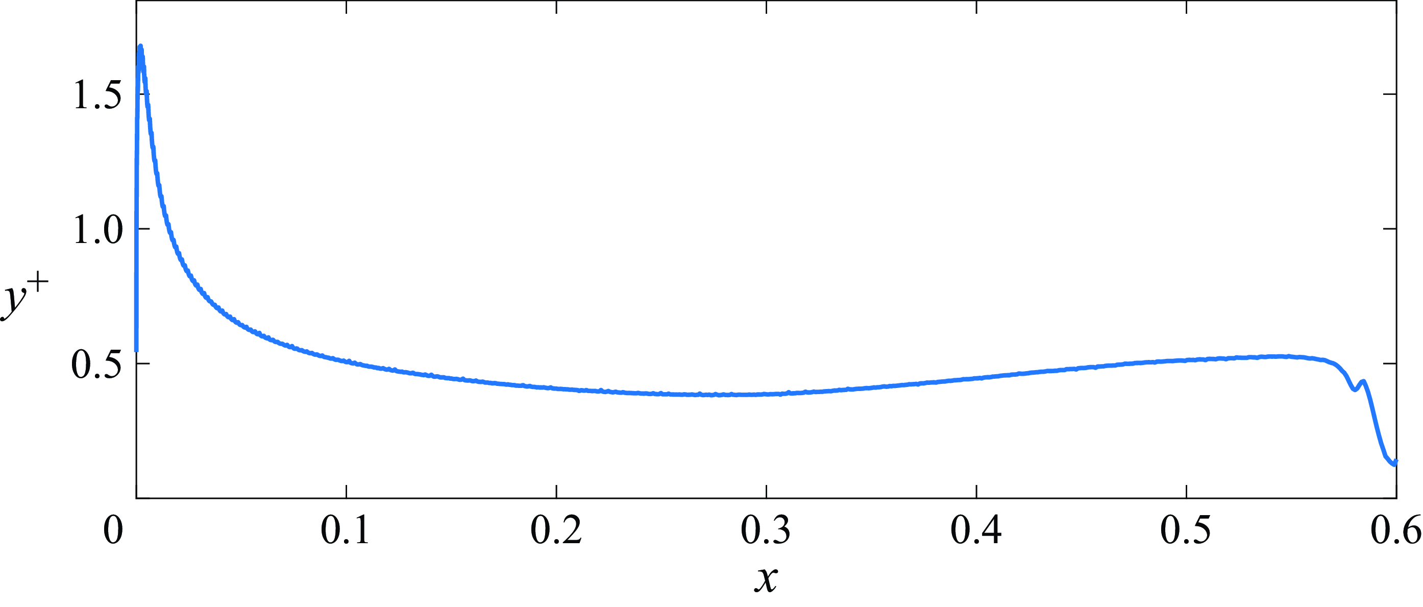
Concerning the mesh resolution, the
 $y^+$
values for the nonlinear case are plotted as a function of streamwise position in figure 2. Since Nek5000 is a spectral elements solver, the actual resolution is smaller than the individual element’s size and, in order to compute
 $y^+$
, we take
 $y=L_e/N_p$
, where
 $L_e$
is the size of the element closest to the wall and
 $N_p=7$
is the polynomial order of the simulation. It should be noted that this is a conservative estimation, since the GLL quadrature has points clustered at the edges of the elements, resulting in an even higher resolution near the airfoil’s wall.
Figure 3 shows snapshots of the streamwise wall-shear stress fluctuations,
 $\tau ^\prime _w = ({1}/{{Re}}) ({\partial u_s^\prime }/{\partial n})$
, where
 $u_s$
is the streamwise velocity fluctuation component parallel to the wall, at the same time step for both linear and nonlinear simulations. By comparing these two plots, we can see the different responses at the wall when nonlinear effects are considered. In particular, high amplitude streaks with short spanwise wavelength appear in the nonlinear case. Moreover, by averaging the
 $\tau ^\prime _w$
of the nonlinear simulation in time and span (figure 4), we can estimate that the boundary layer begins to transition at around
 $x = 0.2$
, with the wall stress growing downstream until in reaches the sponge region near the end of the domain.
Mesh resolution at the wall for the nonlinear simulation, measured in
 $y^+$
units. For this calculation, we estimate
 $y=L_e/N_p$
, where
 $L_e$
is the size of the element closest to the wall and
 $N_p=7$
is the polynomial order of the simulation.

Snapshots of the streamwise wall-shear stress fluctuations,
 $\tau ^\prime _w = ({1}/{{Re}}) ({\partial u_s^\prime }/{\partial n})$
, taken at the same arbitrary time step. (a) Linear simulation. (b) Nonlinear simulation.

Streamwise wall-shear stress fluctuations of the nonlinear simulation averaged in time and span. Transition to turbulence occurs downstream of position
 $x=0.2$
, where
 $\tau ^\prime _w$
increases.

3. Analysis techniques
3.1. Input–output formulation
The linearised input–output model is constructed within the resolvent framework (Jovanović & Bamieh Reference Jovanović and Bamieh2005; Hwang & Cossu Reference Hwang and Cossu2010; McKeon & Sharma Reference McKeon and Sharma2010) by separating the velocity field,
 $\boldsymbol{u}$
, into two main components: a base flow,
 $\boldsymbol{U}$
, and fluctuations around it,
 ${\boldsymbol{u}}^{\prime }$
, such that
 $\boldsymbol{u} = \boldsymbol{U} + {\boldsymbol{u}}^{\prime }$
, and treating the nonlinear convective terms as an external input to the system. The base flow is a 2-D, time-invariant laminar solution,
 $\boldsymbol{U} = [U(x,y),V(x,y),0 ]^{T}$
, while fluctuations are described as a full vector field,
 ${\boldsymbol{u}}^{\prime } = [u^\prime (t,x,y,z),v^\prime (t,x,y,z),w^\prime (t,x,y,z) ]^{T}$
.
Using Einstein’s summation, we write the incompressible NS equations in perturbation form around
 $\boldsymbol{U}$
as
 \begin{equation} \left . \begin{array}{c} \dfrac {\partial u^\prime _i}{\partial t} + U_j \dfrac {\partial u^\prime _i}{\partial x_j} + u^\prime _j \dfrac {\partial U_i}{\partial x_j} + \dfrac {\partial p^\prime }{\partial x_i} - \dfrac {1}{{Re}} \dfrac {\partial ^2 u^\prime _i}{\partial x_j \partial x_j} = f_i + \zeta _i, \\[10pt] \dfrac {\partial u^\prime _j}{\partial x_j} = 0, \end{array}\!\! \right \} \end{equation}
where we group the nonlinear convective terms in
 $f_i = - u^\prime _j (\partial u^\prime _i/\partial x_j )$
and other external terms in
 $\zeta _i$
, comprising the fringe forcing and the inlet turbulence. Then, the NS system can be discretised and rewritten in state-space form
 \begin{equation} \left . \begin{array}{c} \unicode{x1D63D} \dfrac {\partial {\boldsymbol{u}}^{\prime }}{\partial t} + \unicode{x1D647} \boldsymbol{q} = \unicode{x1D63D} \left ( {\zeta } + \boldsymbol{f} \right )\!,\\[4pt] {\boldsymbol{u}}^{\prime } = \unicode{x1D643} \boldsymbol{q}, \end{array}\!\! \right \} \end{equation}
where
 $\boldsymbol{q} = [u^\prime ,v^\prime ,w^\prime ,p^\prime ]^{T}$
,
 $\boldsymbol{\zeta } = [\zeta _x,\zeta _y,\zeta _z]^{T}$
and
 $\boldsymbol{f} = [f_x,f_y,f_z]^{T}$
. Here, the operator
 $\unicode{x1D647}$
encapsulates all time-independent terms from the left-hand side of (3.1) and depends on the spatial discretisation scheme. Operators
 $\unicode{x1D63D}$
and
 $\unicode{x1D643}$
are defined as
 \begin{equation} \unicode{x1D63D} =\left [\!\! \begin{array}{ccc} \unicode{x1D644} & \unicode{x1D655} & \unicode{x1D655} \\ \unicode{x1D655} & \unicode{x1D644} & \unicode{x1D655} \\ \unicode{x1D655} & \unicode{x1D655} & \unicode{x1D644} \\ \unicode{x1D655} & \unicode{x1D655} & \unicode{x1D655} \end{array}\! \right ]\!, \quad \unicode{x1D643} =\left [ \!\!\begin{array}{cccc} \unicode{x1D644} & \unicode{x1D655} & \unicode{x1D655} & \unicode{x1D655} \\ \unicode{x1D655} & \unicode{x1D644} & \unicode{x1D655} & \unicode{x1D655} \\ \unicode{x1D655} & \unicode{x1D655} & \unicode{x1D644} & \unicode{x1D655} \end{array}\! \right ]\!, \end{equation}
where
 $\unicode{x1D644}$
and
 $\unicode{x1D655}$
are the identity and zero matrices of the appropriate size. By exploiting the principle of linear superposition, the differential equation can be decomposed into a system excited by the external forcing acting on the boundaries and fringe
 \begin{equation} \left . \begin{array}{c} \unicode{x1D63D} \dfrac {\partial {\boldsymbol{u}}^{\prime}_{\boldsymbol{L}}}{\partial t} + \unicode{x1D647} \boldsymbol{q_L} = \unicode{x1D63D} \boldsymbol{\zeta }, \\[8pt] {\boldsymbol{u}}^{\prime}_{\boldsymbol{L}} = \unicode{x1D643} \boldsymbol{q_L}, \end{array}\!\! \right \} \end{equation}
and a system excited by the volumetric nonlinear convective forcing
 \begin{equation} \left . \begin{array}{c} \unicode{x1D63D} \dfrac {\partial {\boldsymbol{u}}^{\prime}_{\boldsymbol{N}}}{\partial t} + \unicode{x1D647} \boldsymbol{q_N} = \unicode{x1D63D}\boldsymbol{f},\\[8pt] {\boldsymbol{u}}^{\prime}_{\boldsymbol{N}} = \unicode{x1D643} \boldsymbol{q_N}, \end{array}\!\! \right \} \end{equation}
implying that
 \begin{equation} {\boldsymbol{u}}^{\prime } = {\boldsymbol{u}}^{\prime}_{\boldsymbol{L}} + {\boldsymbol{u}}^{\prime}_{\boldsymbol{N}}. \end{equation}
Here, the vector
 ${\boldsymbol{u}}^{\prime }$
in (3.2) is the velocity field corresponding to the solution of the full NS system, while the vector
 ${\boldsymbol{u}}^{\prime}_{\boldsymbol{L}}$
in (3.4) represents the solution to the linearised NS system subject to the same inlet and boundary conditions. Therefore, through the subtraction of the linearised solution from the full solution, we obtain the velocity field response,
 ${\boldsymbol{u}}^{\prime}_{\boldsymbol{N}}$
solely due to the nonlinear signal
 $\boldsymbol{f}$
.
We perform a Fourier transform in time to obtain from (3.5) the relation
 \begin{equation} \left . \begin{array}{r} \left (\boldsymbol{\varOmega }+\unicode{x1D647}\right ) \boldsymbol{\hat {q}_N} = \unicode{x1D63D} \boldsymbol{\hat {f}}, \\[4pt] \boldsymbol{\hat {u}_N} = \unicode{x1D643} \boldsymbol{\hat {q}_N}, \end{array}\!\! \right \}\!, \quad \boldsymbol{\varOmega } = -i \omega \left [ \!\!\begin{array}{cccc} \unicode{x1D644} & \unicode{x1D655} & \unicode{x1D655} & \unicode{x1D655} \\ \unicode{x1D655} & \unicode{x1D644} & \unicode{x1D655} & \unicode{x1D655} \\ \unicode{x1D655} & \unicode{x1D655} & \unicode{x1D644} & \unicode{x1D655} \\ \unicode{x1D655} & \unicode{x1D655} & \unicode{x1D655} & \unicode{x1D655} \end{array}\! \right ]\!, \end{equation}
as a function of frequency,
 $\omega$
. The nonlinear response,
 $\boldsymbol{\hat {u}_N}$
, and the nonlinear forcing,
 $\boldsymbol{\hat {f}}$
, are related in Fourier space by the resolvent operator
 \begin{equation} \unicode{x1D64D} = \unicode{x1D643}\left (\boldsymbol{\varOmega }+\unicode{x1D647}\right )^{-1} \unicode{x1D63D}\, \implies \boldsymbol{\hat {u}_N} = \unicode{x1D64D} \boldsymbol{\hat {f}}. \end{equation}
The existence of the resolvent operator allows for the application of the resolvent-extended spectral POD framework (Karban et al. Reference Karban, Martini, Cavalieri, Lesshafft and Jordan2022), which will be detailed in § 3.4.
In the work of Blanco et al. (Reference Blanco, Hanifi, Henningson and Cavalieri2024), a single NS simulation was performed, with the need for the construction of the linear operators
 $\unicode{x1D643}$
,
 $\boldsymbol{\varOmega }$
,
 $\unicode{x1D647}$
and
 $\unicode{x1D63D}$
in matrix form to separate linear and nonlinear responses. In particular, the construction of matrix
 $\unicode{x1D647}$
is an especially sensitive operation, since it requires the application of boundary conditions and the knowledge of spatial derivative matrices that are dependent on the mesh and often impractical to build for large simulations and complex geometries.
The procedure presented here is analogous. The difference, however, resides in the fact that
 ${\boldsymbol{u}}^{\prime}_{\boldsymbol{N}}$
can be computed in the time domain before the application of the Fourier transform due to the existence of two simulations, a DNS and a corresponding linearised solution. This, in turn, avoids the explicit construction of any linear operator in matrix form, since these are effectively embedded in the time stepping within the numerical solver. The present approach can thus be applied to arbitrary geometries and boundary conditions, provided that a time stepper (solver) for the full nonlinear and linearised Navier–Stokes systems is available.
3.2. Data processing
In the present study, the computation of
 ${\boldsymbol{u}}^{\prime}_{\boldsymbol{L}}$
,
 ${\boldsymbol{u}}^{\prime}_{\boldsymbol{N}}$
and
 $\boldsymbol{f}$
is achieved by performing two separate simulations. We run a DNS of the NACA0008 airfoil (nonlinear case) in parallel with a linearised version of the same case around a previously computed laminar base flow (linear case), mimicking the time evolution of inlet conditions, boundary conditions and fringe parameters of the full case. Let
 $\boldsymbol{u}(t,x,y,z)$
be the velocity field from the nonlinear case,
 $\boldsymbol{U}(x,y)$
the laminar base flow and
 ${\boldsymbol{u}}^{\prime}_{\boldsymbol{L}}(t,x,y,z)$
the velocity field from the linear case, we have
 \begin{equation} {\boldsymbol{u}}^{\prime } = \boldsymbol{u} - \boldsymbol{U}, \end{equation}
and therefore
 \begin{align}&\quad {\boldsymbol{u}}^{\prime}_{\boldsymbol{N}} = {\boldsymbol{u}}^{\prime } - {\boldsymbol{u}}^{\prime}_{\boldsymbol{L}}, \end{align}
 \begin{align}& \boldsymbol{f} = -( {\boldsymbol{u}}^{\prime } \boldsymbol{\cdot}\boldsymbol{\nabla }) {\boldsymbol{u}}^{\prime }, \end{align}
where
 $\boldsymbol{f}$
is computed employing functions already implemented in the solver (see Appendix A).
As shown in § 2, the fields corresponding to
 ${\boldsymbol{u}}^{\prime }$
and
 ${\boldsymbol{u}}^{\prime}_{\boldsymbol{L}}$
are saved at the same time steps. The saved data are Fourier transformed in the periodic direction,
 $\boldsymbol{z}$
, and organised for each wavenumber,
 $\beta$
, into data matrices containing row-wise stacked components and
 $N_t$
columns corresponding to the number of saved snapshots
 \begin{align} \boldsymbol{\tilde {u}} = \text{FFT}_z \{{\boldsymbol{u}}^{\prime }\}, \\[-28pt] \nonumber \end{align}
 \begin{align} \boldsymbol{\tilde {\unicode{x1D650}}_{\unicode{x1D647}}} = \left [\!\! \begin{array}{ccc} \mid & & \mid \\ \boldsymbol{\tilde {u}_L^{(1)}} & {\cdots} & \boldsymbol{\tilde {u}_L^{(N_t)}} \\ \mid & & \mid \end{array}\!\!\right ]\!, \: \boldsymbol{\tilde {\unicode{x1D650}}_{\unicode{x1D649}}} = \left [ \!\!\begin{array}{ccc} \mid & & \mid \\ \boldsymbol{\tilde {u}_N^{(1)}} & {\cdots} & \boldsymbol{\tilde {u}_N^{(N_t)}} \\ \mid & & \mid \end{array}\!\!\right ]\!, \\[-28pt] \nonumber \end{align}
 \begin{align} \boldsymbol{\tilde {\unicode{x1D641}}} = \left [\!\! \begin{array}{ccc} \mid & & \mid \\ \boldsymbol{\tilde {f}^{(1)}} & {\cdots} & \boldsymbol{\tilde {f}^{(N_t)}} \\ \mid & & \mid \end{array}\!\!\right ]\!. \\[6pt] \nonumber \end{align}
Examples of snapshots for variables
 $\boldsymbol{\tilde {u}_L}$
,
 $\boldsymbol{\tilde {u}_N}$
and
 $\boldsymbol{\tilde {f}}$
are shown in figure 5.
Snapshots of the
 $x$
component of
 $\boldsymbol{\tilde {u}_L}$
(a),
 $\boldsymbol{\tilde {u}_N}$
(b) and
 $\boldsymbol{\tilde {f}}$
(c) at an arbitrary time,
 $t$
, and spanwise wavenumber,
 $\beta$
. The real part of the fields is shown in the panels. Note that the boundary conditions, and especially the inlet condition, for
 $\boldsymbol{\tilde {u}_L}$
and
 $\boldsymbol{\tilde {u}_N}$
are the same.

Further, we apply the spectral estimation algorithm presented in Towne, Schmidt & Colonius (Reference Towne, Schmidt and Colonius2018) to assemble the spectral data matrices, for each pair
 $(\beta ,\omega )$
, containing
 $N_b$
columns which correspond to the number of blocks used within the Welch (Reference Welch1967) method
 \begin{align}&\qquad\qquad\qquad\qquad\quad \boldsymbol{\hat {u}} = \text{Welch}\left \{\boldsymbol{\tilde {u}}\right \}\!, \end{align}
 \begin{align}& \boldsymbol{\hat {\unicode{x1D650}}_{\unicode{x1D647}}} = \left [ \!\!\begin{array}{ccc} \mid & & \mid \\ \boldsymbol{\hat {u}_L^{(1)}} & {\cdots} & \boldsymbol{\hat {u}_L^{(N_b)}} \\ \mid & & \mid \end{array}\right ]\!, \: \boldsymbol{\hat {\unicode{x1D650}}_{\unicode{x1D649}}} = \left [ \!\!\begin{array}{ccc} \mid & & \mid \\ \boldsymbol{\hat {u}_N^{(1)}} & {\cdots} & \boldsymbol{\hat {u}_N^{(N_b)}} \\ \mid & & \mid \end{array}\!\!\right ]\!, \end{align}
 \begin{align}&\qquad\qquad\qquad \boldsymbol{\hat {\unicode{x1D641}}} = \left [ \!\!\begin{array}{ccc} \mid & & \mid \\ \boldsymbol{\hat {f}^{(1)}} & {\cdots} & \boldsymbol{\hat {f}^{(N_b)}} \\ \mid & & \mid \end{array}\!\!\right ]\!. \end{align}
As in Blanco et al. (Reference Blanco, Hanifi, Henningson and Cavalieri2024), the windowing function is set as
 \begin{equation} w(t) = \sin \left (\frac {\pi t}{T}\right )\!, \quad t \in [0,T] ,\end{equation}
with
 $3/4$
overlap between consecutive blocks (Antoni & Schoukens Reference Antoni and Schoukens2009). For each case (linear and nonlinear) we obtained a total of
 $N_t=2100$
snapshots of fully developed flow, equally spaced by
 $\Delta t = 2.5 \times 10^{-3}$
time units,
 $\tau = c/U_{\infty }$
. Here,
 $c$
is the unitary chord length and
 $U_{\infty }$
the free-stream velocity. In all the analyses, the spectral estimation was performed using
 $N_b=34$
data blocks of
 $N_{\textit{FFT}} = 256$
snapshots each. Theses parameters yield a sampling frequency of
 $f_s = 400 \: \tau ^{-1}$
and a frequency resolution of
 $\Delta f = f_s/N_{\textit{FFT}} = 1.5625 \: \tau ^{-1}$
. The statistical convergence arising from this choice of parameters is discussed in Appendix B.
3.3. Flow statistics from data
We take the Fourier transform in time and span of (3.6) and subsequently substitute the spectral data matrices from (3.16) and (3.17) to write
 \begin{equation} \boldsymbol{\hat {\unicode{x1D650}}} = \boldsymbol{\hat {\unicode{x1D650}}}_{\unicode{x1D647}} + \boldsymbol{\hat {\unicode{x1D650}}_{\unicode{x1D649}}}. \end{equation}
The cross-spectral density (CSD) matrix of matrix
 $\boldsymbol{\hat {\unicode{x1D650}}}$
can be estimated from the computed data as
 \begin{equation} \boldsymbol{\hat {\unicode{x1D63E}}_{\unicode{x1D650}\unicode{x1D650}}} (\beta ,\omega ) = \frac {1}{N_b} \boldsymbol{\hat {\unicode{x1D650}}}\boldsymbol{\hat {\unicode{x1D650}}}^H = \frac {1}{N_b} (\boldsymbol{\hat {\unicode{x1D650}}_{\unicode{x1D647}}} + \boldsymbol{\hat {\unicode{x1D650}}_{\unicode{x1D649}}}) (\boldsymbol{\hat {\unicode{x1D650}}_{\unicode{x1D647}}} + \boldsymbol{\hat {\unicode{x1D650}}_{\unicode{x1D649}}})^H, \end{equation}
where
 $\left \{\boldsymbol{\cdot }\right \}^H$
denotes the conjugate transpose, and is further expanded in the form
 \begin{align} \boldsymbol{\hat {\unicode{x1D63E}}_{\unicode{x1D650}\unicode{x1D650}}} &= \boldsymbol{\hat {\unicode{x1D63E}}_{\unicode{x1D650}\unicode{x1D650}_{\unicode{x1D647}}}} + \boldsymbol{\hat {\unicode{x1D63E}}_{\unicode{x1D650}\unicode{x1D650}_{\unicode{x1D649}}}}, \end{align}
 \begin{align} \boldsymbol{\hat {\unicode{x1D63E}}_{\unicode{x1D650}\unicode{x1D650}_{\unicode{x1D647}}}} &= \boldsymbol{\hat {\unicode{x1D63E}}_{\unicode{x1D650}_{\unicode{x1D647}} \unicode{x1D650}_{\unicode{x1D647}}}} + \boldsymbol{\hat {\unicode{x1D63E}}_{\unicode{x1D650}_{\unicode{x1D649}} \unicode{x1D650}_{\unicode{x1D647}}}}, \nonumber\\ \boldsymbol{\hat {\unicode{x1D63E}}_{\unicode{x1D650}\unicode{x1D650}_{\unicode{x1D649}}}} &= \boldsymbol{\hat {\unicode{x1D63E}}_{\unicode{x1D650}_{\unicode{x1D647}} \unicode{x1D650}_{\unicode{x1D649}}}} + \boldsymbol{\hat {\unicode{x1D63E}}_{\unicode{x1D650}_{\unicode{x1D649}} \unicode{x1D650}_{\unicode{x1D649}}}}. \end{align}
The relation presented in (3.21) quantifies how much each component (linear or nonlinear) affects the DNS velocity perturbation spectrum. In practice,
 $\boldsymbol{\hat {\unicode{x1D63E}}_{\unicode{x1D650}\unicode{x1D650}}}$
is not computed since it contains a number of elements equal to the square of the number of mesh points, making it difficult to store in memory and manipulate. Instead, we focus on the power spectral density (PSD), a real and positive vector defined as the diagonal of the CSD. We rewrite (3.21) as a pointwise budget relation
 \begin{equation} \underbrace {\text{diag} (\boldsymbol{\hat {\unicode{x1D63E}}_{\unicode{x1D650}\unicode{x1D650}}})}_{\boldsymbol{P_U}} = \underbrace {{{Re}} \{\text{diag} (\boldsymbol{\hat {\unicode{x1D63E}}_{\unicode{x1D650}\unicode{x1D650}_{\unicode{x1D647}}}})\}}_{\boldsymbol{\varPi _L}} + \underbrace {{{Re}} \{\text{diag} (\boldsymbol{\hat {\unicode{x1D63E}}_{\unicode{x1D650}\unicode{x1D650}_{\unicode{x1D649}}}}) \}}_{\boldsymbol{\varPi _N}} ,\end{equation}
where
 ${{Re}}\left \{\boldsymbol{\cdot }\right \}$
and
 $\text{diag} (\boldsymbol{\cdot })$
denote, respectively, the real part and diagonal of the matrix. This allows us to identify, for a given pair of
 $(\beta , \omega )$
, where the kinetic energy results from either linear or nonlinear mechanisms, or even a combination of both. It is important to note that
 $\boldsymbol{\hat {\unicode{x1D63E}}_{\unicode{x1D650}\unicode{x1D650}_{\unicode{x1D647}}}}$
and
 $\boldsymbol{\hat {\unicode{x1D63E}}_{\unicode{x1D650}\unicode{x1D650}_{\unicode{x1D649}}}}$
are not Hermitian matrices since they incorporate cross-multiplications of components. This implies that, even though
 $\boldsymbol{P_U}$
is a pointwise PSD,
 $\boldsymbol{\varPi _L}$
and
 $\boldsymbol{\varPi _N}$
are not and therefore can assume either positive or negative values, interpreted as inflows or outflows of energy at a given wavenumber and frequency, as in Blanco et al. (Reference Blanco, Hanifi, Henningson and Cavalieri2024).
3.4. Proper orthogonal decomposition
Once the pairs
 $(\beta , \omega )$
of interest are identified, we can perform a spectral POD analysis (Towne et al. Reference Towne, Schmidt and Colonius2018) by computing the eigenvalues of the corresponding CSD matrix,
 $\boldsymbol{\hat {\unicode{x1D63E}}_{\unicode{x1D650}\unicode{x1D650}}}$
, to visualise the most energetic structures involved in the dynamics.
If the energy analysis yields a dynamics induced predominantly through the nonlinear forcing, the resolvent-based extended POD (RESPOD) (Karban et al. Reference Karban, Martini, Cavalieri, Lesshafft and Jordan2022) method is applied to compute the spectral POD modes of the response and the corresponding nonlinear forcing modes. With this, we can construct a ranked modal decomposition of the forcing statistics, a powerful tool to model and analyse coherent structures identified to be generated through the nonlinear interactions.
The RESPOD method is applied through the following steps. First, we substitute the data matrices from (3.16) and (3.17) into (3.8). Due to the windowing employed in the spectral estimation, an extra correction term,
 $\boldsymbol{\hat {\unicode{x1D641}}_{\unicode{x1D658}}}$
, is introduced (Martini et al. Reference Martini, Cavalieri, Jordan and Lesshafft2020; Nogueira et al. Reference Nogueira, Morra, Martini, Cavalieri and Henningson2021) and the dynamical system is written as
 \begin{equation} \boldsymbol{\hat {\unicode{x1D650}}_{\unicode{x1D649}}} = \unicode{x1D64D} (\boldsymbol{\hat {\unicode{x1D641}}} + \boldsymbol{\hat {\unicode{x1D641}}_{\unicode{x1D658}}} ). \end{equation}
Next, we define an augmented state
 \begin{equation} \boldsymbol{\hat {\unicode{x1D64C}}} = \left [ \begin{array}{c} \boldsymbol{\hat {\unicode{x1D650}}_{\unicode{x1D649}}} \\ \boldsymbol{\hat {\unicode{x1D641}}} + \boldsymbol{\hat {\unicode{x1D641}}_{\unicode{x1D658}}} \end{array} \right ]\!, \end{equation}
and compute the weighted CSD matrix
 $\boldsymbol{\hat {\unicode{x1D648}}_{\unicode{x1D64C}}}$
in the row space of
 $\boldsymbol{\hat {\unicode{x1D64C}}}$
as
 \begin{equation} \boldsymbol{\hat {\unicode{x1D648}}_{\unicode{x1D64C}}} = \frac {1}{N_b} \boldsymbol{\hat {\unicode{x1D64C}}}^H \left [ \begin{matrix} \unicode{x1D652} & 0 \\ 0 & 0 \end{matrix} \right ] \boldsymbol{\hat {\unicode{x1D64C}}} = \frac {1}{N_b} {\boldsymbol{\hat {\unicode{x1D650}}^H_{\unicode{x1D649}}}} \unicode{x1D652} \boldsymbol{\hat {\unicode{x1D650}}_{\unicode{x1D649}}}, \end{equation}
where
 $\unicode{x1D652}$
is a diagonal matrix containing the quadrature weights. Following the snapshot algorithm (Sirovich Reference Sirovich1987), we solve the eigenproblem
 \begin{equation} \boldsymbol{\hat {\unicode{x1D648}}_{\unicode{x1D64C}}} \boldsymbol{\varTheta } = \boldsymbol{\varTheta } \boldsymbol{\varLambda }, \end{equation}
such that the resulting POD modes
 $\boldsymbol{\varPsi }$
and associated extended POD modes, also called RESPOD forcing modes,
 $\boldsymbol{\varPhi }$
, can be written as
 \begin{equation} \boldsymbol{\tilde {\varPsi }} = \left [ \begin{matrix} \boldsymbol{\varPsi } \\ \boldsymbol{\varPhi } \end{matrix} \right ] = \frac {1}{\sqrt {N_b}} \boldsymbol{\hat {\unicode{x1D64C}}} \boldsymbol{\varTheta } \boldsymbol{\varLambda }^{-1/2}, \end{equation}
and obey the resolvent relation
 \begin{equation} \boldsymbol{\varPsi } = \unicode{x1D64D} \boldsymbol{\varPhi }, \end{equation}
without the need to explicitly construct the resolvent operator. Therefore, this procedure yields the spectral POD modes of flow fluctuations,
 $\boldsymbol{\varPsi }$
, representing coherent structures that dominate flow fluctuations, and associated forcing modes,
 $\boldsymbol{\varPhi }$
, which excite them. Further details on the theory and algorithms for computing the correction due to windowing,
 $\boldsymbol{\hat {\unicode{x1D641}}_{\unicode{x1D658}}}$
, and the RESPOD modes,
 $\boldsymbol{\tilde {\varPsi }}$
, are presented in Blanco et al. (Reference Blanco, Hanifi, Henningson and Cavalieri2024).
It must be emphasised that there is a practical benefit in computing RESPOD forcing modes rather than directly obtaining the spectral POD modes of the forcing data. As outlined in (3.29), each forcing mode
 $\boldsymbol{\varPhi }$
is mapped and synchronised in spanwise phase via the resolvent operator to a single response mode,
 $\boldsymbol{\varPsi }$
. This allows for the computation of a low-rank decomposition of the nonlinear forcing signal by selecting a corresponding low-rank set of response modes. In contrast, computing the spectral POD of the forcing data results in modes that, when projected through the resolvent operator, map to multiple response modes (Morra et al. Reference Morra, Nogueira, Cavalieri and Henningson2021), complicating the derivation of a low-rank representation of the nonlinear forcing that is dynamically linked to the most energetic flow structures.
4. Secondary instabilities as triggers to turbulence
As commonly found in FST-induced transition, the boundary layer is populated by irregular streaks at different stages of their development. Therefore, their breakdown is also irregular, happening scattered in time and space along the boundary layer. Regardless of their scattered appearance, it has been shown that streak secondary instabilities play a significant role in bypass transition breakdown (Matsubara & Alfredsson Reference Matsubara and Alfredsson2001; Mans, De Lange & Van Steenhoven Reference Mans, De Lange and Van Steenhoven2007; Schlatter et al. Reference Schlatter, Brandt, de Lange and Henningson2008; Hack & Zaki Reference Hack and Zaki2014). More recently, Faúndez Alarcón et al. (Reference Faúndez Alarcón, Cavalieri, Hanifi and Henningson2024) showed that secondary instabilities were the main cause of turbulent spots’ inception in a flat plate and, therefore, the main source for transition in their simulation.
Example of secondary instability. The top plot shows the full span at
 $x=0.25$
, with the contour representing the streamwise velocity perturbation from the DNS. The black and white open contours correspond to the negative and positive streamwise components, respectively, of the secondary instability computed using the equations in Appendix C. The bottom right plot shows a zoomed view centred around the unstable streak. The grey contours in the bottom left plot correspond to the shear at the wall from the DNS at the spanwise position
 $z\approx 1.9 \times 10^{-2}$
, with the blue dot indicating the time and streamwise position for the stability calculation.

We perform local stability analyses in planes upstream of turbulent spots nucleation and at previous time steps to identify the breaking streaks. Here, we follow the same procedure as the one used in Faúndez Alarcón et al. (Reference Faúndez Alarcón, Cavalieri, Hanifi and Henningson2024), where more details about the formulation can be found. The extracted planes contain the full DNS solution, which is used as the base flow for the stability calculations. Here, a parallel flow assumption is invoked due to the slow streamwise variation of the flow composed of a 2-D time-invariant solution plus low-frequency streaks. Moreover, streak secondary instabilities are characterised as high-frequency waves relative to the streaks, which further justifies the parallel assumption in their study. For completeness, the stability equations are included in Appendix C.
Figure 6 depicts an example of an unstable mode, with streamwise wavenumber
 $\alpha =800$
and complex frequency
 $\omega =699.2 + 11.2i$
, before a turbulent spot nucleation. We note that two unstable modes were found at this plane, both on top of the same low-speed streak, but only the one with the highest growth rate is shown. The blue dot in the time–space diagram represents the time instant and streamwise position where the DNS plane was extracted and its stability analysis performed. At later times of the stability calculation, and consistently with the phase speed of the unstable modes, a turbulent spot is nucleated which is then convected and spread downstream.
The example shown in figure 6 is a typical representation of what we have observed in this simulation, with secondary instabilities appearing in low-speed streaks with relatively short spanwise wavelength. The realisation that the breakdown to turbulence is driven by the secondary stabilities of streaks at higher spanwise wavenumbers guides the choice of parameters considered in the analyses performed in the following sections.
5. Energy budget
The first analysis of this work concerns the distribution of the kinetic energy of perturbations over the frequency and spanwise wavenumber spectra, as well as their evolution over the airfoil. Since we are interested in the receptivity phenomena occurring within a laminar, transitional region, we consider a region near the leading edge that avoids the turbulent spots occurring further downstream, as shown in figure 7. Furthermore, we separate the region inside and outside the boundary layer by applying a mask
 ${\unicode{x1D652}}_{\unicode{x1D63D}\unicode{x1D647}}$
, shown in figure 8, with the same shape as the matrix
 $\unicode{x1D652}$
presented in (3.26). The edge of the boundary layer is defined at the vorticity threshold of
 $\text{vort}_z = 0.01 \: \text{vort}_{z,w\textit{all}}$
, where
 $\text{vort}_{z,w\textit{all}}$
is the vorticity of the laminar base flow at the nearest wall point.
In black, the contour of the region considered for energy integration. It is chosen to avoid the turbulent spots occurring downstream on the airfoil.

Boundary-layer mask. The boundary-layer edge is set at the vorticity threshold
 $\text{vort}_z = 0.01 \: \text{vort}_{z,w\textit{all}}$
. The transition between inside and outside the boundary layer is modelled as a smooth step function with a value of 0.5 at the edge position.

From flow data, we compute the pointwise quantities
 $\boldsymbol{\varPi _L}$
and
 $\boldsymbol{\varPi _N}$
described in § 3.3. Then, we integrate over those
 $N$
points which lay within the previously defined region to obtain the linear and nonlinear contributions to the perturbation kinetic energy,
 $E$
 \begin{align}&\quad\,\, E_{L,\textit{in}}(\beta ,\omega ) = \sum _{i = 1}^{N} \left ({\unicode{x1D652}}_{\unicode{x1D63D}\unicode{x1D647}} \unicode{x1D652} \boldsymbol{\varPi _L}\right )_i\!, \end{align}
 \begin{align}& E_{L,out}(\beta ,\omega ) = \sum _{i = 1}^{N} \left (\left (\unicode{x1D644}-{\unicode{x1D652}}_{\unicode{x1D63D}\unicode{x1D647}}\right )\unicode{x1D652}\boldsymbol{\varPi _L}\right )_i\!, \end{align}
 \begin{align}&\quad\,\, E_{N,\textit{in}}(\beta ,\omega ) = \sum _{i = 1}^{N} \left ({\unicode{x1D652}}_{\unicode{x1D63D}\unicode{x1D647}}\unicode{x1D652} \boldsymbol{\varPi _N}\right )_i\!, \end{align}
 \begin{align}& E_{N,\textit{out}}(\beta ,\omega ) = \sum _{i = 1}^{N} \left (\left (\unicode{x1D644}-{\unicode{x1D652}}_{\unicode{x1D63D}\unicode{x1D647}}\right )\unicode{x1D652}\boldsymbol{\varPi _N}\right )_i\!, \end{align}
where the matrix
 $\unicode{x1D652}$
denotes the quadrature weights, such that
 \begin{equation} E = \sum _{i = 1}^{N} \left ( \unicode{x1D652} \boldsymbol{P_U}\right )_i = E_{L,\textit{in}} + E_{L,out} + E_{N,\textit{in}} + E_{N,out}. \end{equation}
We sweep the calculations over all pairs
 $(\beta ,\omega )$
and compile the results in figure 9, where energies for negative spanwise wavenumbers are not shown since
 $E(\beta ,\omega ) = E(-\beta ,-\omega )$
for real-valued signals.
Spectra of linear and nonlinear energy contributions, inside and outside the boundary layer. For each plot, pairs
 $(\beta ,\omega )$
are listed in descending order of magnitude, excluding the base flow distortion at
 $(0,0)$
. In the
 $E_{L,out}$
plot, the spectrum of the FST field imposed at the inlet is superposed on the spectrum. Colours in symlog scale (Webber Reference Webber2012).

In the free stream, the energy peaks of the linear component are discretely distributed, coinciding with the also discrete FST spectrum imposed at the inlet because the linear dynamics is locked and does not transfer energy between different time and space scales. It is also observed that the FST introduces the most energy in perturbations of low
 $(\beta ,\omega )$
, with no energy present at
 $\beta =0$
by design. However, this does not imply that the flow cannot possess an energy component at this wavenumber. In reality, the convective terms of the NS equations interact across multiple wavenumbers and frequencies, ultimately transferring energy to
 $\beta =0$
. In the boundary layer, this manifests as an energy peak at
 $(\beta ,\omega )=(0,0)$
, the base flow distortion, which captures the deviation between the measured mean flow and the prescribed laminar base flow. On the top of this mean flow, fluctuations with highest energy occur at the peaks shown in figure 9.
Conversely, in the free stream, the nonlinear terms smoothly distribute the energy of the imposed FST across the spectrum. The blue regions in the
 $E_N$
component indicate that the excess energy introduced via the
 $E_L$
component is transferred away from the low-frequency and wavenumber region.
The spectrum is quite different inside the boundary layer since the energy distribution is highly biased toward lower frequencies. This reflects the phenomenon called shear sheltering (Hunt & Carruthers Reference Hunt and Carruthers1990; Hunt & Durbin Reference Hunt and Durbin1999), in which the boundary layer prevents the penetration of higher-frequency perturbations. Moreover, it reinforces the boundary layer’s tendency to amplify low-frequency structures, corroborating the results from optimal growth analysis (Andersson et al. Reference Andersson, Berggren and Henningson1999; Luchini Reference Luchini2000). Within the linear component of the spectrum,
 $E_L$
, energy peaks at the already cited low
 $(\beta ,\omega )$
range are created through the linear advection of the perturbations introduced by the FST.
Upon inspecting figure 9, contrasting features are observed between the linear,
 $E_{L,\textit{in}}$
and nonlinear,
 $E_{N,\textit{in}}$
, components inside the boundary layer. In the linear component, the energy peak is found at the first two spanwise wavenumbers above zero (
 $\beta =89.363$
and
 $\beta =178.752$
) while in the nonlinear component the most important energy inflows are situated at
 $\beta \approx 500$
. By computing the associated wavelength of this wavenumber, we get
 $\lambda = 2 \pi / \beta = 2\pi / 500 \approx 0.012$
, which, in turn, yields streaky structures of size around
 $\varDelta z = 0.006$
(one wavelength contains one positive streak and one negative streak). Incidentally, the secondary stability analysis of § 4 identified streaks in this size range (figure 6) as sources of turbulent spots. This observation implies that the near-wall structures ultimately decaying to turbulence in the simulation are not linearly induced by the FST spectrum, but rather generated through nonlinear interactions. However, the energy budget analysis does not identify where the source of these nonlinear interactions is situated. In other words, the budget alone does not identify if the nonlinear mechanisms capable of generating the measured streaks are active inside or outside the boundary layer.
In a further investigation, we focus on the boundary layer and integrate
 $E_{L,\textit{in}}$
and
 $E_{N,\textit{in}}$
over all available frequencies and at each station along the airfoil’s upper surface, in figure 10. The results corroborate that the energy of the first two wavenumbers above zero is primarily due to linear mechanisms. In contrast, the rest of the wavenumbers are influenced by nonlinear dynamics. This effect is particularly strong at
 $\beta =0$
, responsible for base flow distortions, at which no energy is injected via the FST perturbation field. One crucial observation concerns the region near
 $x=0$
. Even though energy is only introduced to the boundary layer at certain wavenumbers, the nonlinear component smoothly distributes energy at the leading edge over the full range of wavenumbers. This could imply that nonlinear interactions affecting the development of turbulence over the airfoil happen, at least in part, upstream of the wing’s stagnation point.
Evolution of energy components integrated inside the boundary layer, over all frequencies, over different stations at the airfoil’s upper surface.

The data collected through the energy budget directs the analyses developed in the subsequent sections of this work. Since nonlinearity is perceived to play an essential role in amplifying the near-zero frequency streaks responsible for the generation of turbulence over the airfoil, we focus our next analyses on the stationary pairs of
 $E_{N,\textit{in}}$
which add energy to the flow within the boundary layer. These are the pairs at
 $\omega =0$
at the
 $E_{N,\textit{in}}$
spectrum component which have negligible linear counterpart, shown inside the grey-shaded region in figure 11. A more detailed study of these stationary components of the flow allows for a description of the mean nonlinear forcing signal related to turbulent transition.
Zero-frequency (time-stationary) slice of the
 $E_{\textit{in}}$
spectrum component. (a) Full range of spanwise wavenumbers. (b) Zoom on the grey-shaded region, showing the spanwise wavenumbers of
 $E_{N,\textit{in}}$
that add energy to the stationary flow. Here, we exclude the mean-flow distortion measured at
 $(\beta ,\omega ) = (0,0)$
. Y-axis in symlog scale, the same as in figure 9.

6. Modal analysis
6.1. Spatial distribution
We focus on the pairs
 $(\beta ,\omega ) = (446.813,0.000)$
and
 $(\beta ,\omega ) = (536.176,0.000)$
, whose energies are mainly a result of nonlinear interactions as seen in figure 11. The observed separation of at least one order of magnitude indicates that
 $\boldsymbol{P_U} \approx \boldsymbol{\varPi _N}$
and thus linear mechanisms can be neglected in this case. Moreover, the spatial distribution of
 $\boldsymbol{\varPi _N}$
implies that nonlinearly induced structures are only meaningful within the near-wall region, with the bulk of the energy located within the shear region of the base flow inside the boundary layer.
The data presented in figures 12 and 13 enable the identification of regions where nonlinear perturbations dominate. In this context, nonlinearity indicates that the observed energy does not arise from the linear amplification of perturbations advected from the inlet by the base flow. Instead, it emerges as a superposition of responses from the linearised system, driven by the nonlinear volumetric input field acting across all points in the domain. Consequently, determining the spatial origin of nonlinear interactions is not straightforward through an energy budget analysis alone.
Components of
 $\boldsymbol{P_U}$
for
 $(\beta ,\omega )=(446.813,0.000)$
. (a,b) Full region. (c,d) Zoom at the leading edge. Note that
 $\boldsymbol{\varPi _L}$
is two orders of magnitude smaller than
 $\boldsymbol{\varPi _N}$
.

Components of
 $\boldsymbol{P_U}$
for
 $(\beta ,\omega )=(536.176,0.000)$
. (a,b) Full region. (c,d) Zoom at the leading edge. Note that
 $\boldsymbol{\varPi _L}$
is one order of magnitude smaller than
 $\boldsymbol{\varPi _N}$
.

6.2. Low-rank dynamics
The RESPOD method, introduced in § 3.4, is employed to effectively analyse nonlinear forcing characteristics beyond the energy budget. For the specific
 $(\beta ,\omega )$
pair under consideration, we calculate the data matrices
 $\boldsymbol{\hat {\unicode{x1D650}}_{\unicode{x1D649}}}$
,
 $\boldsymbol{\hat {\unicode{x1D641}}}$
and
 $\boldsymbol{\hat {\unicode{x1D641}}_{\unicode{x1D63E}}}$
in order to construct the augmented state vector
 $\unicode{x1D64C}$
of (3.25). Since we are only interested in the coherent structures developing near the airfoil’s surface, we apply the boundary-layer mask from figure 8 to the weights matrix
 \begin{equation} {\unicode{x1D652}_{\boldsymbol{a}}} = \left [ \begin{array}{cc} {\unicode{x1D652}}_{\unicode{x1D63D}\unicode{x1D647}} \unicode{x1D652} & 0 \\[4pt] 0 & 0 \end{array} \right ]\!, \end{equation}
such that all the points in the free stream have their integration weights zeroed out. In practice, this means that only correlations within the boundary layer are considered to compute the modal decomposition. The decomposition coefficients can then be used to extend the POD modes to the full numerical domain (Borée Reference Borée2003).
Results are displayed in figures 14 to 16. From figure 14, the modal analysis shows that the dynamics at the considered wavenumbers and frequency is low rank and can be mostly described by the first response and forcing modes, shown in figures 15 and 16, since the largest eigenvalue captures more than 85 % of the total energy in both cases.
Eigenvalues (energies) associated with each RESPOD mode. The first eigenvalue captures 92 % of the total energy for the pair
 $(\beta ,\omega )=(446.813,0.000)$
and 86 % for the pair
 $(\beta ,\omega )=(536.176,0.000)$
. Note that the same eigenvalue is shared between forcing and response modes.

As the budget analysis from § 5 showed, the magnitudes of the response modes in figures 15(a) (left) and 16(a) (left) indicate that the energy of nonlinear perturbations is mostly contained within the region near the boundary layer. The structures amplified downstream of the studied region are indeed streaks, as shown in figures 15(b) (top) and 16(b) (top): streamwise elongated structures composed of alternating regions of slow and fast flow accompanied by intercalated counter-rotating streamwise vortices. When the vortex carries fluid towards the wall it generates a fast streak, while a slow streak is created when fluid is lifted from the surface. Hence, the label lift-up effect (Landahl Reference Landahl1980).
The spatial distributions of the magnitude of the forcing mode, shown in figures 15(a) (right) and 16(a) (right), indicate that the nonlinear forcing is active in the region near the airfoil, where it continuously feeds energy into the boundary layer. However, contrary to the response, the forcing mode also has a significant presence upstream of the leading edge. Since the FST introduced at the boundary is discretely distributed over wavenumbers and frequencies, the turbulent velocity field will inevitably redistribute the energy into a smoother spectrum. In other words, we perceive the turbulent energy cascade (Moffatt Reference Moffatt2014) responsible for the accommodation of the FST spectrum as forcing structures appearing directly downstream of the inlet.
When the alignments between response and forcing modes are calculated by computing their Euclidean inner product
 $\langle {\boldsymbol{\cdot}},{\boldsymbol{\cdot }}\rangle$
, illustrated in figures 15(b) (bottom) and 16(b) (bottom), the data reveal a significant component that opposes the streaks within the boundary layer (blue regions in the
 $\langle {\boldsymbol{u_s}},{\boldsymbol{f_s}}\rangle$
field), which points to the presence of a nonlinear mechanism draining the energy of streaks, within the boundary layer. Conversely, the forcing energises the streamwise counter-rotating vortices from outside the boundary layer. This effect is evident from the red regions in the
 $\langle \boldsymbol{u}_{\boldsymbol{\parallel} \boldsymbol{(}{\boldsymbol{n}},{\boldsymbol{z}}\boldsymbol{ )}},{\boldsymbol{f}_{\boldsymbol{\parallel} \boldsymbol{(}{\boldsymbol{n}},{\boldsymbol{z}} \boldsymbol{)}}}\rangle$
field, which indicate a positive alignment between the response and forcing around the streaks, particularly above them. It is important to recall that linear growth theory (Andersson et al. Reference Andersson, Berggren and Henningson1999; Luchini Reference Luchini2000) identifies streamwise vortices as an optimal forcing. Therefore, even though the nonlinear forcing acts in a non-optimal manner by removing energy, it still contributes to the growth of streaks within the boundary layer. In this scenario, the amplification mechanism aligns with that described by linear theory, but the receptivity process differs. Here, streamwise vortices are continuously sustained and energised across the boundary layer, rather than reaching their peak intensity near the leading edge of the wing and subsequently decaying. These observations are consistent with the earlier findings of Blanco et al. (Reference Blanco, Hanifi, Henningson and Cavalieri2024).
7. Receptivity
7.1. Reference position for the receptivity analysis
The receptivity mechanisms are generally analysed with respect to the perturbations that actually reach the boundary layer or the leading edge of the wing. This feature contrasts with the framework of the present study, which identifies linear and nonlinear mechanisms concerning the perturbation field introduced at the inlet boundary, situated further upstream of the airfoil’s leading edge.
The RESPOD modes in figures 15(a) and 16(a) confirm the presence of nonlinear forcing upstream of the airfoil. This is supported by the mismatch in streaky structures at the leading edge between linear and nonlinear simulations previously seen in figures 3 and 5. Concerning the nonlinear case, this demonstrates that the imposed Fourier modes at the inlet do not fully dictate the near-airfoil flow. Instead, nonlinear interactions smoothly redistribute the energy across the wavenumbers, leading to deviations in the energy spectrum measured at the leading edge and quantified by the component
 $E_{N,\textit{in}}$
in figure 10.
Although this upstream forcing is weaker in magnitude compared with the forcing near the airfoil, the perturbations it generates can be linearly amplified once they reach the airfoil’s shear region. In this case, mechanisms typically linked to linear receptivity are instead embedded within the nonlinear energy spectrum. Once the reference position was changed from the one traditionally used in receptivity analyses, from the leading edge to the inlet, any conclusions about linearity is also shifted accordingly.
7.2. Forced linear system
To bring the analysis from the inlet to the wing’s leading edge and measure the linearity of responses considering the reference point usually adopted in receptivity studies, at the leading edge, we can resort back to the numerical solver. Considering that the dynamics of the pairs
 $(\beta ,\omega ) = (446.813,0.000)$
and
 $(\beta ,\omega ) = (536.176,0.000)$
is similar, we focus on the first one. The previous analyses showed that the flow is dominated by the nonlinear response and given that
 $\varPsi _1 = \unicode{x1D64D} \varPhi _1$
from (3.29), we can feed the expanded forcing mode from nonlinear simulations,
 $\boldsymbol{f_1}=\varPhi _1 \: e^{i (\beta z - \omega t )}$
, as the sole external force input of the linearised solver to obtain a reconstructed solution field,
 $\boldsymbol{u_{\!R}}$
. This, by construction, is equivalent to the expanded response mode,
 $\boldsymbol{u_1}=\varPsi _1 \: e^{i (\beta z - \omega t )}$
, even though deviations might appear due to spectral estimation and numerical errors. By employing the linearised solver to reconstruct an already computed response, we can restrict the forcing input to certain domain regions. For instance, we can force only the region upstream of the leading edge (figure 17) to account for the accommodation of the FST spectrum and evaluate the linear downstream propagation of perturbations reaching the leading edge. Conversely, we can obtain information concerning the effects of the nonlinear forcing acting over the airfoil by restricting the input to positions downstream of the leading edge. Because the system is linearised, the sum of these two effects must be equivalent to the RESPOD response mode.
Leading RESPOD modes for
 $(\beta ,\omega )=(446.813,0.000)$
. (a) Magnitude of RESPOD modes scaled by the corresponding eigenvalue,
 $\lambda_1$
. (i)
 $\Psi_1$
. (ii)
 $\Phi_1$
. (b) Slice perpendicular to the airfoil, at position x = 0.15. Directions n and s are, respectively, normal to the surface and streamwise. From top to bottom: (i)
 $\Psi_1$
. (ii)
 $\Phi_1$
. (iii) Alignment between streamwise components of response and forcing. (iv) Alignment between non-streamwise components of response and forcing, where
 $\langle{\boldsymbol{\cdot}}, {\boldsymbol{\cdot}} \rangle$
denotes inner product.

Leading RESPOD modes for
 $(\beta ,\omega )=(536.176,0.000)$
. (a) Magnitude of RESPOD modes scaled by the corresponding eigenvalue,
 $\lambda_{1}$
. (i)
 $\Psi_{1}$
. (ii)
 $\Phi_{1}$
. (b) Slice perpendicular to the airfoil, at position x = 0.15. Directions n and s are, respectively, normal to the surface and streamwise. From top to bottom: (i)
 $\Psi_{1}$
. (ii)
 $\Phi_{1}$
. (iii) Alignment between streamwise components of response and forcing. (iv) Alignment between non-streamwise components of response and forcing.

Upstream mask. Nonlinear interactions are active upstream of the leading edge and deactivated once they reach the airfoil.

Computing
 $\boldsymbol{u_{\!\textit{R}}}$
implies running the time stepper, with the same boundary conditions presented in § 3, until transient effects have dissipated and the solution has converged to a single-frequency harmonic response in time. In the convenience of
 $\omega =0$
, as is the case, the simulation should run until the stationary solution converges. The stop threshold chosen for this study is
 $L^2$
norm between consecutive iterations below
 $10^{-8}$
.
7.3. Response reconstruction
In the first analysis step, we input the full forcing mode into the linearised solver. The result obtained is displayed in figure 18. The reconstructed velocity field is close to the expanded response mode in a visual comparison. The isosurfaces show streaks synchronised in phase and of approximately the same amplitude. Moreover, a quantitative comparison, performed by computing the normalised projection between vectors, yields
 \begin{equation} \frac {\boldsymbol{u^T_1} \boldsymbol{u_{\!\textit{R}}}}{\boldsymbol{u^T_1}\boldsymbol{u_1}} = 0.91, \end{equation}
where
 $\{\boldsymbol{\cdot }\}^T$
denotes transposed. An alignment close to 1 between
 $\boldsymbol{u_1}$
and
 $\boldsymbol{u_{\!\textit{R}}}$
means both are similar in shape and magnitude. It demonstrates the efficacy of the proposed procedures, from the spectral estimation to the statistical convergence of POD modes, and, above all, attests to the accuracy of the calculations done so far, at least for the studied pair
 $(\beta ,\omega )$
. Further considerations on the convergence of the method are presented in Appendix B.
Isosurfaces of the
 $x$
component of velocity corresponding to values
 $\pm 0.003$
. The reconstructed response is close to the expanded RESPOD mode.

Next, we run the linearised solver again, this time applying the upstream mask (figure 17) to the forcing field. This approach enables us to isolate and analyse the component of the response that arises from the free-stream development upstream of the leading edge, specifically capturing the streaks generated by this upstream influence. Since the solved system is linear, the resulting velocity field is then subtracted from the one shown in figure 18(a) to obtain the equivalent of the response to a downstream masked forcing. The three obtained responses, to full, upstream-masked forcing (UMF) and downstream-masked forcing (DMF) fields, are then compared in figure 19. Results show that the velocity field over the airfoil in further downstream positions is equally influenced by either UMF or DMF fields. Most importantly, both forcing fields generate streaks inside the boundary layer (figure 19 a).
From figure 19(b), it is evident that the UMF response exhibits a faster growth rate near the leading edge. The velocity field is characterised by strong perturbations in the
 $n$
and
 $z$
directions close to position
 $x=0$
, which tend to decay further downstream, while the streamwise velocity component,
 $\boldsymbol{u}_{{\boldsymbol{s}},{\boldsymbol{rms}}}$
steadily increases, showing a tendency to stabilise downstream. In contrast, the DMF response has a negligible amplitude near the leading edge, with all three velocity components demonstrating growth across the entire studied range. Specifically,
 $\boldsymbol{u}_{{\boldsymbol{s}},{\boldsymbol{rms}}}$
displays a slower initial growth rate compared with the UMF case. However, the DMF fluctuations continue to grow further downstream and eventually surpass the UMF streaks. Since the amplitude slope of the DMF remains positive at the end of the domain, we anticipate further growth due to nonlinear forcing in downstream regions.
Comparison between full, UMF and DMF responses. Directions
 $n$
and
 $s$
are, respectively, wall normal and streamwise. (a) Velocity field at a slice perpendicular to the surface, passing by position x = 0.2. (i) Full response; (ii) UMF response; (iii) DMF response. (b) Evolution of velocity perturbations over the airfoil. The amplitude is defined as the square root of the energy integrated inside the boundary layer.

7.4. Receptivity mechanisms
The features observed in the UMF response can be studied in more details by looking at the perturbations at the leading edge, displayed in figure 20(a). Near the stagnation point, the turbulence advected from the free stream induces perturbations in
 $\boldsymbol{u_n}$
and
 $\boldsymbol{u_z}$
, which, in turn, generate counter-rotating vortices in front of the airfoil. These vortices bend around the leading edge (figure 20
b), align with the streamwise direction and decay monotonically downstream while streaks grow, an effect that can be clearly verified by the decay of components
 $\boldsymbol{u}_{\boldsymbol{n},\boldsymbol{rms}}$
and
 $\boldsymbol{u}_{\boldsymbol{z},\boldsymbol{rms}}$
of the UMF response, accompanied by the increase in
 $\boldsymbol{u}_{{\boldsymbol{s}},{\boldsymbol{rms}}}$
, as shown in figure 19(b). This constitutes an efficient mechanism of streak amplification, a known result of optimal growth analysis (Andersson et al. Reference Andersson, Berggren and Henningson1999; Luchini Reference Luchini2000; Schrader et al. Reference Schrader, Brandt, Mavriplis and Henningson2010).
By definition, the DMF response is not influenced directly by the scales of the incoming turbulence. Rather, it receives energy from different scales of motion, through nonlinear interactions. Streaks are not amplified by an initial condition at the leading edge. Instead, they are continuously induced over the entire airfoil surface by a volumetric forcing resulting from said nonlinear interactions, which explains the steady growth of components
 $\boldsymbol{u}_{\boldsymbol{n},\boldsymbol{rms}}$
and
 $\boldsymbol{u}_{\boldsymbol{z},\boldsymbol{rms}}$
of the DMF response in figure 19(b). This same phenomenon has been described by Blanco et al. (Reference Blanco, Hanifi, Henningson and Cavalieri2024) for the case of a flat plate without a leading edge. Most importantly, these results corroborate the previous findings from Sasaki et al. (Reference Sasaki, Cavalieri, Hanifi and Henningson2022) stating that streaky structures can be generated solely by forcing outside the boundary layer, whose optimal response corresponds to non-streamwise velocity ‘growing along the streamwise direction, as they are continuously driven by the forcing component’.
The UMF response. (a) Velocity field at slice perpendicular to the surface, passing by the leading edge. Note the coordinate equivalence:
 $(s,n,z) = (y,-x,z)$
. (b) Vortices (green), represented by
 $\lambda _2$
structures, and streaks (red and blue).

The forcing field over the wing, depicted previously in figure 16, operates both inside and outside the boundary layer. Inside, the forcing removes energy while feeding vortices from the outside. Physically, this suggests that the nonlinear mechanisms in the current scenario may involve triadic interactions either between streaks within the boundary layer or between streaks and structures outside the boundary layer. An example of the first case from the literature is the
 $\beta$
-cascading process described in Henningson, Lundbladh & Johansson (Reference Henningson, Lundbladh and Johansson1993) and Henningson (Reference Henningson1996), where wider streaks (lower
 $\beta$
, slower transient growth) transfer energy into thinner streaks (higher
 $\beta$
, comparatively faster transient growth). For the second case, a potential scenario involves the oblique waves discussed in Berlin et al. (Reference Berlin, Wiegel and Henningson1999), which have been shown to generate streaks in both numerical and experimental set-ups, through vortices penetrating the boundary layer. Unfortunately, the energy budget formulation applied to this study is limited to quantifying the energy inflows and outflows for a given pair
 $(\beta ,\omega )$
, without identifying the origin or destination of these transfers. As a result, a detailed description of the specific mechanisms at play remains a topic for future research.
By separating the forcing into distinct regions, one upstream of the leading edge and another downstream, we can pinpoint the origin of the measured responses. The UMF response corresponds to the portion of the nonlinear response arising from the development of the FST before the wing. It represents a form of linear receptivity because once the turbulence reaches the wing, the UMF ceases, and the flow can only see the linear amplification of perturbations induced by initial conditions set at the airfoil’s leading edge. In contrast, the DMF response results from the continuous nonlinear interaction between the free stream over the wing and the boundary layer, illustrating a nonlinear receptivity. Now, the energy that amplifies perturbations is drawn into the boundary layer from other scales of motion, mathematically described as different wavenumber and frequencies from those corresponding to the structures measured in the most energetic response mode. Finally, since we are dealing with a linearised system, we can just add UMF and DMF responses to obtain the full flow field.
8. Discussion
The identification of two distinct receptivity mechanisms of equal relative importance is aligned with the findings in Faúndez Alarcón et al. (Reference Faúndez Alarcón, Morra, Hanifi and Henningson2022). At higher FST levels, nonlinear interactions are non-negligible and induce a profile of amplification over the wing that deviates from the linear theory. While linear receptivity is more active in the regions near the leading edge, due to the presence of the FST-induced streamwise vortices generated at the stagnation point, nonlinear receptivity is not present in the initial stages of the boundary-layer development and only reaches comparable amplification levels farther downstream. Since these two mechanisms are present at roughly different regions over the wing (upstream and downstream), we can conjecture that their relative importance within the streak amplification phase will affect transition location.
For low FST level cases, Faúndez Alarcón et al. (Reference Faúndez Alarcón, Morra, Hanifi and Henningson2022) showed that the streaks growing in the boundary layer have scales which are correlated with the scales of the free-stream fluctuations measured near the leading edge and streak amplitude is well predicted by projecting the measured disturbances into the optimal growth modes. Therefore, optimal disturbance theory (Andersson et al. Reference Andersson, Berggren and Henningson1999; Luchini Reference Luchini2000) can explain trends in streak growth and spanwise scale. In this scenario, receptivity happens further upstream, close to the leading edge, without the pronounced effect of continuous forcing over the airfoil.
However, the situation may differ when considering high FST-level and large integral length scale environments. High FST levels induce stronger nonlinear interactions (Blanco et al. Reference Blanco, Hanifi, Henningson and Cavalieri2024), while larger scales are related to the slower decay of the FST over the airfoil, making it more effective in continuously forcing disturbances inside the boundary layer (Brandt Reference Brandt2014). In this case, the streaks responsible for the generation of turbulent spots will have a different characteristic spanwise wavenumber than the ones where the most kinetic energy was introduced by the FST, as seen in § 5 of this study. As a further indication of this effect, figure 10 clearly shows that
 $E_{N,\textit{in}}$
removes energy from the most energetic spanwise wavenumbers in
 $E_{L,\textit{in}}$
when composing the full spectrum,
 $E_{\textit{in}}$
.
Finally, the present study is, to our best knowledge, the first to demonstrate that receptivity in a realistic set-up of a wing with leading edge subject to a high level FST can be the product of both linear and nonlinear mechanisms. In the case studied, we arrive at the important conclusion that transition is triggered by streaky structures resulting from nonlinear receptivity mechanisms. This is, in fact, a departure from current understanding from transient growth theory that FST generated streaks grow rapidly and tend to decay if a certain critical amplitude, capable of triggering secondary instabilities, is not reached. Instead, streaks and associated streamwise vortices are measured to be constantly growing in amplitude, highlighting the importance of free-stream interactions within the boundary layer downstream of the leading edge even in early stages of transition.
9. Conclusions
In order to identify contributions from linear and nonlinear forcing to growth of the boundary-layer perturbations, we have performed two numerical simulations. One DNS and one linearised Navier–Stokes simulation around a laminar base flow, both exposed to the same boundary and inflow conditions. The study is based on the case presented in Faúndez Alarcón et al. (Reference Faúndez Alarcón, Morra, Hanifi and Henningson2022) and was devised to analyse receptivity mechanisms on a NACA0008 airfoil subject to a
 $\textit{Tu}=2.5\,\%$
level of FST.
We compute the difference between the velocity perturbation fields of the DNS and linearised simulation. This nonlinear response,
 ${\boldsymbol{u}}^{\prime}_{\boldsymbol{N}}$
, is by construction exclusively the result of the nonlinear forcing term
 $\boldsymbol{f} = - ({\boldsymbol{u}}^{\prime } \boldsymbol{\cdot }\boldsymbol{\nabla }) {\boldsymbol{u}}^{\prime }$
computed from DNS perturbations,
 ${\boldsymbol{u}}^{\prime }$
.
Once these data are obtained, we compute the energy budget by integrating the contributions of linear and nonlinear responses,
 ${\boldsymbol{u}}^{\prime}_{\boldsymbol{L}}$
(coming from the linearised case) and
 ${\boldsymbol{u}}^{\prime}_{\boldsymbol{N}}$
respectively, over the transitional region near the leading edge. Results show that the streaks identified as generators of turbulent spots by Faúndez Alarcón et al. (Reference Faúndez Alarcón, Morra, Hanifi and Henningson2022) are not the result of the advection of the inflow perturbations, but are rather caused by the energy redistribution promoted by the nonlinear terms, with minimal linear influence. Also, the evolution of the energy spectrum over the airfoil shows that the DNS and linearised simulation differ in the distribution of energy at the leading edge, with the DNS containing more energy at higher wavenumbers.
We identify the pairs
 $(\beta ,\omega )=(446.813,0.000)$
and
 $(446.813,0.000)$
as a representative wavenumber on the nonlinear component of the spectrum inside the boundary layer and use it to perform a RESPOD analysis. The results show that the dynamics at this scale is low rank, with more than 85 % of the energy captured by the first spectral POD mode. This response mode mainly concentrates the kinetic energy over the airfoil, with little activity in the free stream. The coherent structures generated are indeed streaks, with their characteristic alternating regions of slow and fast streamwise flow, intercalated by counter-rotating vortices. However, the corresponding forcing mode shows important features before the leading edge. It implies that the spectrum at the leading edge differs from the one introduced at the inlet boundary, due to the energy redistribution occurring upstream.
In order to study the receptivity mechanisms, we mask the forcing mode into two zones: upstream of the leading edge, allowing us to account for the accommodation of the FST spectrum, and downstream of it. This allows us to compute the responses to either forcing separately. Results show that both linear receptivity, due to the upstream forcing, and nonlinear mechanisms, due to the continuously active forcing downstream, are important for the amplification of perturbations inside the boundary layer. Moreover, both generate streaks as a forced response. These findings, highlight the importance of free-stream interactions with the boundary layer downstream of the leading edge even in early stages of transition.
Acknowledgements
The computations were performed on resources provided by The National Academic Infrastructure for Supercomputing in Sweden (NAISS) at NSC. We would like to thank S. Kern for the fruitful discussions related to the work developed here, especially concerning questions related to the Nek5000 solver.
Funding
This work has been financially supported by Fundação de Amparo à Pesquisa do Estado de São Paulo, FAPESP, under grants nos. 2019/27655-3, 2020/14200-5 and 2022/01424-8; Vinnova through the NFFP project LaFloDes (grant number 2019-05369); the European Research Council (grant agreement 694452-TRANSEP-ERC-2015-AdG); and the Swedish e-Science Research Centre (SeRC).
Declaration of interests
The authors report no conflict of interest.
Appendix A. Convective forcing data
As stated in § 2, the BDF2/EXT2 time integration scheme employed within the numerical solver is semi-implicit, meaning that the linear diffusive terms of the NS system are treated implicitly while the convective terms are treated explicitly.
In version 19 of Nek5000, the subroutine convop, inside the navier1.f file, is responsible for the explicit computation of the convection of a passive scalar,
 $\phi$
, by a given velocity field,
 $\boldsymbol{u}$
, in the skew-symmetric form (Blaisdell, Spyropoulos & Qin Reference Blaisdell, Spyropoulos and Qin1996). The subroutine applies multiple numerical techniques to reduce the aliasing errors arising from the advection and inherent nonlinearity of the NS equations, including over-integration (Malm et al. Reference Malm, Schlatter, Fischer and Henningson2013). To overcome the insufficient quadrature, the fields are interpolated into spectral elements containing
 $1.5\times$
more points, with the resulting convective term being interpolated back to the polynomial order of the simulation. This work adapted the convop subroutine to accept the perturbation field,
 ${\boldsymbol{u}}^{\prime }$
, from (3.9), instead of the full velocity field of the DNS. Therefore, the computation of the convective forcing terms and the subsequent analyses could be carried out with the same level of spectral precision as in the numerical solver.
Appendix B. On the convergence of the proposed methods
The resolvent-based spectral POD procedure presented in § 3.4 relies on the Welch method for the estimation of the power spectrum, which has well-defined formulas for the calculation of confidence bounds (Welch Reference Welch1967).
Assuming that velocity fluctuations at a given point have a Gaussian distribution in time and ignoring the effects of the employed windowing function, the confidence interval of the spectral estimation can be computed as
 \begin{equation} \frac {D}{\chi ^2_{\textit{in}v}(D,1-\alpha /2)} \hat {P}(\omega ) \leqslant P(\omega ) \leqslant \frac {D}{\chi ^2_{\textit{in}v}(D,\alpha /2)} \hat {P}(\omega ), \end{equation}
where
 $D = 2 N_{\textit{FFT}}$
is the number of degrees of freedom,
 $\chi ^2_{\textit{in}v}$
is the inverse
 $\chi ^2$
cumulative distribution function,
 $\alpha = 1 - C$
, with
 $C$
denoting the confidence level required,
 $\hat {P}(\omega )$
is the estimated PSD and
 $P(\omega )$
the true PSD. As stated in § 3.2, the spectral estimation was performed using
 $N_b=34$
data blocks of
 $N_{\textit{FFT}} = 256$
snapshots each. By substituting these parameters in (B1) we have
 \begin{equation} 0.734 \: \hat {P}(\omega ) \leqslant P(\omega ) \leqslant 1.444 \: \hat {P}(\omega ), \end{equation}
for a confidence level of 95 %, which is a relatively wide interval.
Narrowing this interval is challenging because running a very long DNS is prohibitively expensive. Additionally, increasing the number of Welch blocks by reducing snapshots per block results in biased spectral POD modes (Blanco et al. Reference Blanco, Martini, Sasaki and Cavalieri2022). Nevertheless, this does not undermine the analyses in § 5, as the positions of energy peaks in the power spectrum are expected to remain stable within frequency resolution errors.
Concerning the modal analysis introduced in § 6, even though the PSD might not correctly estimate the energy levels, the eigenvalues at the pairs
 $(\beta ,\omega )$
show an expressive separation, with the first mode capturing around 90 % of the total energy. This indicates a good convergence of the POD analysis.
Later, in § 7, we show that the forcing modes – when transformed from Fourier space to the time domain – still accurately reproduce the inputs that generate the observed response modes via the linearised Navier–Stokes operator, further confirming the validity of the performed analyses.
Appendix C. Stability analysis
The stability of the flow field is performed in frozen planes normal to streamwise direction. These planes are extracted from the snapshots of the nonlinear simulation, where the full solution is used as a base flow and therefore taking the form
 $\boldsymbol{U}_{0}(n,z) = [U_{0}(n,z),V_{0}(n,z), W_{0}(n,z)]^{\mathsf{T}}$
. Note that
 $n$
represents the wall’s normal direction at the corresponding chord position. Since turbulent spots appear far from the leading edge, the curvature was neglected and planes perpendicular to the wall are approximated to be vertical. The field is then decomposed as
 \begin{align} \boldsymbol{U}(t,\boldsymbol{x}) &= \boldsymbol{U}_{0}(n,z) + \boldsymbol{u}_2 (t,\boldsymbol{x}) , \end{align}
 \begin{align} P(t,\boldsymbol{x}) &= P_{0}(n,z) + p_2(t,\boldsymbol{x}), \end{align}
where the subscript 2 was added to emphasise that the perturbation corresponds to the secondary instability of the streaky base flow. By assuming a normal mode form for the perturbation
 $\boldsymbol{u}_2(t,\boldsymbol{x})=\hat {\boldsymbol{u}}_2(n,z) \exp (i(\alpha x - \omega t) )$
and the same for the pressure, we linearise the Navier–Stokes equations around
 $\boldsymbol{U}_{0}$
and obtaining
 \begin{align} ({\unicode{x1D63E}}- \varDelta) \hat {u}_2 + ({\unicode{x1D63F}}_y U) \hat {v}_2 + ({\unicode{x1D63F}}_z U ) \hat {w}_2 + i\alpha \hat {p}_2 &= i\omega \hat {u}_2, \end{align}
 \begin{align} ( {\unicode{x1D63E}}- \varDelta + {\unicode{x1D63F}}_yV ) \hat {v}_2 + ({\unicode{x1D63F}}_z V ) \hat {w}_2 + {\unicode{x1D63F}}_y \hat {p}_2 &= i\omega \hat {v}_2, \end{align}
 \begin{align} ({\unicode{x1D63F}}_y W) \hat {v}_2+ ({\unicode{x1D63E}}- \varDelta + {\unicode{x1D63F}}_zW ) \hat {w}_2+ {\unicode{x1D63F}}_z \hat {p}_2 &= i\omega \hat {w}_2, \end{align}
 \begin{align} i \alpha \hat {u}_2 + {\unicode{x1D63F}}_y \hat {v}_2 + {\unicode{x1D63F}}_z \hat {w}_2 &= 0 , \end{align}
where
 \begin{align} {\unicode{x1D63E}} & = U_{0} i\alpha + V_{0} {\unicode{x1D63F}}_y + W_{0}{\unicode{x1D63F}}_z , \end{align}
 \begin{align} \varDelta & =1/{Re} \big({-}\alpha ^2+{\unicode{x1D63F}}_y^{\kern1pt 2} + {\unicode{x1D63F}}_z^{\kern1pt 2} \big) , \end{align}
 \begin{align} {\unicode{x1D63F}}_y & = \partial /\partial y \\[6pt] \nonumber \end{align}
and
 \begin{align} {\unicode{x1D63F}}_z=\partial /\partial z . \end{align}
The differential operators are discretised with a fourth-order finite differences scheme, while zero perturbation is imposed at the wall and in the free stream, and periodicity along the span.