2.1. Governing equations and boundary conditions

We consider two-dimensional flow of incompressible and inviscid fluids, comprising two immiscible fluid layers with constant densities denoted as $\rho _i$ and undisturbed thickness $H_{i}$ . Here, the subscript $i=1$ and $i=2$ are used for variables on the upper- and lower-fluid layers, respectively. 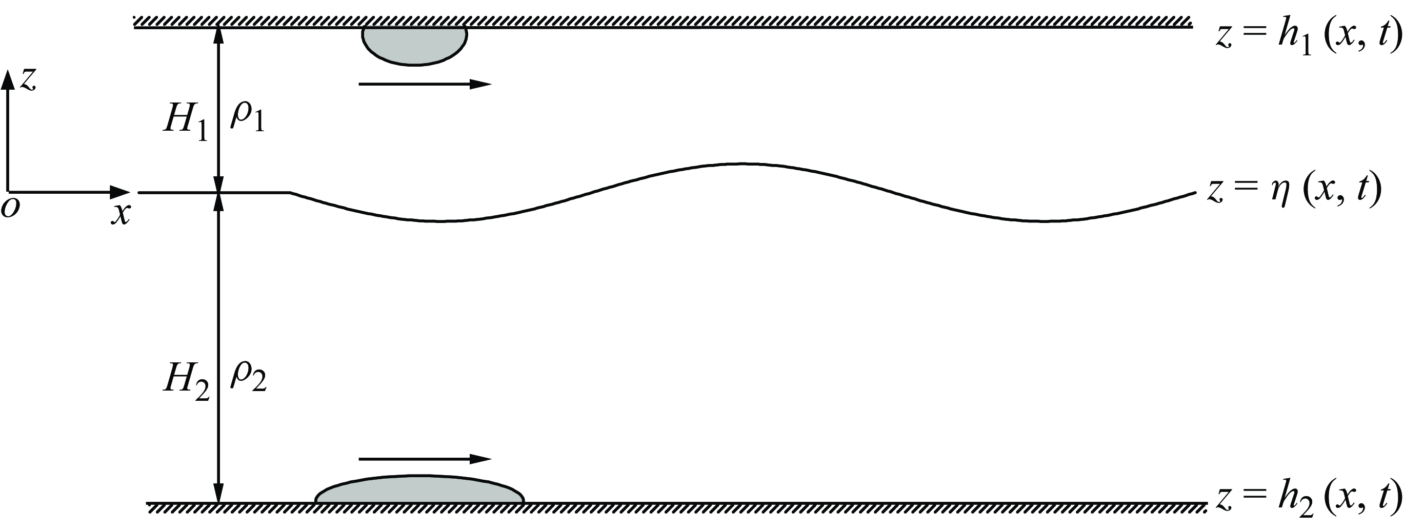The coordinate origin is set at the undisturbed interface, with $x$ denoting the horizontal axis (positive to the right) and $z$ representing the vertical axis (positive upwards). 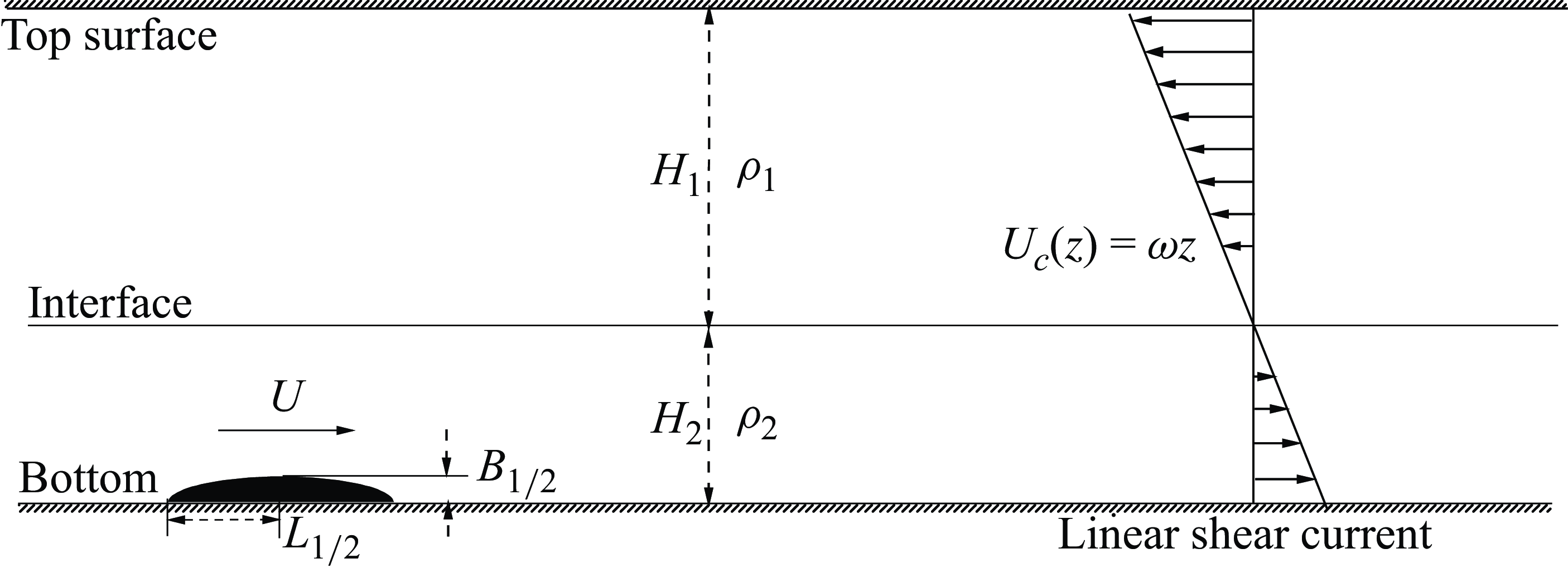Considering the boundaries varying with time, the top-surface elevation, the interface elevation and the bottom elevation are represented by $z=h_1(x,t)$ , $z=\eta (x,t)$ and $z=h_2(x,t)$ , respectively. A sketch of the two-layer fluid system is shown in figure 1.

Figure 1.

Sketch of a two-layer fluid system with time-varying boundaries.

The mass conservation equations of the two fluid layers can be written as

(2.1) \begin{align} \frac {{\partial {u_i}}}{{\partial x}} + \frac {{\partial {w_i}}}{{\partial z}} = 0\,\,\,\,\,(i=1,2), \end{align}

where $u_{i}(x,z,t)$ and $w_{i}(x,z,t)$ represent the horizontal- and vertical-velocity components, respectively.

The momentum conservation equations of the two-fluid layers can be written as

(2.2a) \begin{align} \frac {{\partial {u_i}}}{{\partial t}} + {u_i}\frac {{\partial {u_i}}}{{\partial x}} + {w_i}\frac {{\partial {u_i}}}{{\partial z}} & = - \frac {1}{{{\rho _i}}}\frac {{\partial {p_i}}}{{\partial x}}\,\,\,\,\,(i=1,2), \\[-12pt] \nonumber \end{align}

(2.2b) \begin{align} \frac {{\partial {w_i}}}{{\partial t}} + {u_i}\frac {{\partial {w_i}}}{{\partial x}} + {w_i}\frac {{\partial {w_i}}}{{\partial z}} & = - \frac {1}{{{\rho _i}}} {\frac {{\partial {p_i}}}{{\partial z}} - g}\,\,\,\,\,(i=1,2), \\[9pt] \nonumber \end{align}

where $t$ is the time, $p_{i}(x,z,t)$ is the pressure and $g$ is the gravitational acceleration.

The kinematic boundary conditions for the upper- and lower-fluid layers are written as

(2.3a) \begin{align} w_1 &= \frac {\partial h_1}{\partial t} + u_1 \frac {\partial h_1}{\partial x} \quad \kern1.4pt \text{at } z = h_1(x,t), \\[-12pt] \nonumber \end{align}

(2.3b) \begin{align} w_1 &= \frac {\partial \eta }{\partial t} + u_1 \frac {\partial \eta }{\partial x} \qquad \text{at } z = \eta (x,t), \\[-12pt] \nonumber \end{align}

(2.3c) \begin{align} w_2 &= \frac {\partial \eta }{\partial t} + u_2 \frac {\partial \eta }{\partial x} \qquad \text{at } z = \eta (x,t), \\[-12pt] \nonumber \end{align}

(2.3d) \begin{align} w_2 &= \frac {\partial h_2}{\partial t} + u_2 \frac {\partial h_2}{\partial x} \quad \kern1.4pt \text{at } z = h_2(x,t). \\[9pt] \nonumber \end{align}

The dynamic boundary condition at the interface between the two-fluid layers is written as

(2.4) \begin{align} {\bar p_1} = {\hat p_2}\quad{\textrm {at }}z = {\eta }(x,t). \end{align}

Here $\bar {p}_i$ and $\hat {p}_i$ are the pressure at the lower and upper surfaces of the $i$ th fluid layer, respectively.

2.2. The HLGN model equations

In the two-layer HLGN model (see, e.g. Zhao et al. Reference Zhao, Ertekin, Duan and Webster2016, Reference Zhao, Wang, Duan, Ertekin, Hayatdavoodi and Zhang2020), the horizontal- and vertical-velocity components are described as

(2.5) \begin{align} {u_i}\left ( {x,z,t} \right ) = \sum \limits _{n = 0}^{{K_i}} {{u_{n,i}}\left ( {x,t} \right ){z^n},\qquad{w_i}\left ( {x,z,t} \right ) = \sum \limits _{n = 0}^{{K_i}} {{w_{n,i}}\left ( {x,t} \right ){z^n}} }\quad(i=1,2), \end{align}

where $K_1$ and $K_2$ are the levels of the HLGN model used for the upper-fluid layer and the lower-fluid layer, respectively. Notation HLGN- $K_1$ – $K_2$ denotes the levels used for the upper-fluid layer and lower-fluid layer in the HLGN model, where $K_1$ and $K_2$ are independent of each other. Here $u_{n,1}(x,t)$ , $w_{n,1}(x,t)$ , $u_{n,2}(x,t)$ and $w_{n,2}(x,t)$ are the unknown velocity coefficients that need to be solved as part of the solutions.

Substituting (2.5) into (2.1) results in

(2.6) \begin{align} u_{K_{i},i}=0\,\,\,\,\,\,\,\,\,\,(i=1,2),\,\,\,\,\,\,\,\,\,\,{w_{n,i}} = - \frac {1}{n}\frac {{\partial {u_{n - 1,i}}}}{{\partial x}}\,\,\,\,\,\,\,\,\,\,(n = 1,2, \ldots ,{K_i}). \end{align}

Substituting (2.5) into (2.2), multiplying each term by $z^n\,(n=0,1,\ldots ,K_i)$ and integrating from $\eta$ to $h_1$ to eliminate ${\bar p}_1$ for the upper layer, and from $h_2$ to $\eta$ to eliminate ${\bar p}_2$ for the lower layer, will result in

(2.7a) \begin{align} {M_{n,1}} + \left ( {h_1^n - {\eta ^n}} \right )\frac {\partial }{{\partial x}}\left ( {\frac {{{{\hat p}_1}}}{{{\rho _1}}}} \right ) = 0\;\;\;\;\;\;\;\;\;\;\big(n = n^U = 1,2, \ldots ,{K_1} \big), \\[-12pt] \nonumber \end{align}

(2.7b) \begin{align} {M_{n,2}} + \left ( {{\eta ^n} - {h_{2}^n}} \right )\frac {\partial }{{\partial x}}\left ( {\frac {{{{\hat p}_2}}}{{{\rho _2}}}} \right ) = 0 \;\;\;\;\;\;\;\;\;\;\big(n = n^L =1,2,\ldots ,K_2 \big). \\[9pt] \nonumber \end{align}

Here we denote the indices of the polynomial expansions by $n = n ^ U$ for the upper layer and $n = n ^ L$ for the lower layer, in order to avoid ambiguity. In functions such as $M_{n,i}$ , $E_{n,i}$ , $G_{n,i}$ , the subscript $i$ is already used to distinguish layers. The functions in (2.7) are given by

(2.8a) \begin{align} &{M_{n,1}}=\frac {\partial }{{\partial x}}\left ( {G_{n,1} + gS1_{n,1}} \right ) + nE_{n - 1,1} - {\eta ^n}\frac {\partial }{{\partial x}}\left ( {G_{0,1} + gS1_{0,1}} \right )\!, \\[-12pt] \nonumber \end{align}

(2.8b) \begin{align} &{M_{n,2}}=\frac {\partial }{{\partial x}}\left ( {G_{n,2} + gS1_{n,2}} \right ) + nE_{n - 1,2} - {h_{2} ^n}\frac {\partial }{{\partial x}}\left ( {G_{0,2} + gS1_{0,2}} \right )\!, \\[-12pt] \nonumber \end{align}

(2.8c) \begin{align} &{E_{n,i}} = \sum \limits _{m = 0}^{K_i} {\left ( {\frac {{\partial {u_{m,i}}}}{{\partial t}}{S2_{\textit{mn},i}} + \frac {{\partial {u_{m,i}}}}{{\partial x}}{Q_{\textit{mn},i}} + {u_{m,i}}{H_{\textit{mn},i}}} \right )} \quad(i=1,2), \\[-12pt] \nonumber \end{align}

(2.8d) \begin{align} &{G_{n,i}} = \sum \limits _{m = 0}^{K_i} {\left ( {\frac {{\partial {w_{m,i}}}}{{\partial t}}{S2_{\textit{mn},i}} + \frac {{\partial {w_{m,i}}}}{{\partial x}}{Q_{\textit{mn},i}} + {w_{m,i}}{H_{\textit{mn},i}}} \right )}\quad(i=1,2), \\[-12pt] \nonumber \end{align}

(2.8e) \begin{align} &{Q_{\textit{mn},i}} = \sum \limits _{r = 0}^{K_i} {{u_{r,i}}{S3_{\textit{mrn},i}}},\;\;\;\;\;{H_{\textit{mn},i}} = \sum \limits _{r = 0}^{K_i} {{w_{r,i}}S4_{\textit{mrn},i}}\quad(i=1,2), \\[-12pt] \nonumber \end{align}

(2.8f) \begin{align} &S1_{n,1} = \int _{\eta } ^{h_{1}} {z^n \textrm {d}z},\;\;\;\;\;S1_{n,2} = \int _{h_{2}} ^{\eta } {z^n \textrm {d}z}, \\[-12pt] \nonumber \end{align}

(2.8g) \begin{align} &S2_{mn,1} = \int _{\eta } ^{h_{1}} {z^{m + n} \textrm {d}z},\;\;\;\;\;S2_{mn,2} = \int _{h_{2}} ^{\eta } {z^{m + n} \textrm {d}z}, \\[-12pt] \nonumber \end{align}

(2.8h) \begin{align} &S3_{mrn,1} = \int _{\eta } ^{h_{1}} {z^{m + r + n} \textrm {d}z},\;\;\;\;\;S3_{mrn,2} = \int _{h_{2}} ^{\eta } {z^{m + r + n} \textrm {d}z}, \\[-12pt] \nonumber \end{align}

(2.8i) \begin{align} &S4_{mrn,1} = m\int _{\eta } ^{h_{1}} {z^{m + r + n - 1} \textrm {d}z},\;\;\;\;\;S4_{mrn,2} = m\int _{h_{2}} ^{\eta } {z^{m + r + n - 1} \textrm {d}z}. \\[9pt] \nonumber \end{align}

At this moment, we are interested in describing ${\hat p}_1$ and ${\hat p}_2$ in (2.7) in alternative forms. Based on (2.4) and the relationship between the upper-surface pressure and the lower-surface pressure for the single-layer HLGN model given by Webster, Duan & Zhao (Reference Webster, Duan and Zhao2011), we obtain the following relation:

(2.9) \begin{align} {\hat p_2} = {\bar p_1} = {\rho _1}(G_{0,1} + gS1_{0,1})+{\hat p_1}. \end{align}

Now, setting $n^U=1$ in (2.7a ) and $n^L=1$ (2.7b ), and combining with (2.9), we can eliminate ${\hat p}_1$ and ${\hat p}_2$ to obtain a new equation. Similarly, setting $n^U=1$ in (2.7a ) and $n^L=2$ in (2.7b ), and combining with (2.9), we can eliminate ${\hat p}_1$ and ${\hat p}_2$ to obtain a second new equation. Following the same principle, we can obtain a series of new equations, which can be written as

(2.10) \begin{align} \frac {{{\rho _2M_{n,2}}}}{\rho _1({\eta ^n - h _2^n})} - \frac {{{}{M_{1,1}}}}{{h_1 - \eta }} + {}\frac {\partial }{{\partial x}}\left ( {{G_{0,1}} + g{S1_{0,1}}} \right ) = 0\;\;\;\;\;\;\;\;\;\;(n=n^L=1,2,\ldots ,K_2). \end{align}

On the other hand, fixing $n^U=1$ in (2.7a ), we can eliminate ${\hat p}_1$ for each $n$ couple, e.g. $n^U=1$ and $n^U=2$ , $n^U=1$ and $n^U=3$ , etc., to obtain another series of new equations. These new equations are presented as

(2.11) \begin{align} \frac {{{M_{n,1}}}}{{h_1^n - \eta ^n}} - \frac {{{M_{1,1}}}}{{h_1 - \eta }} = 0\;\;\;\;\;\;\;\;\;\; \big(n=n^U=2,3,\ldots ,K_1 \big). \end{align}

Substituting (2.5) into (2.3) results in

(2.12a) \begin{align} {w_{0,1}} & = \frac {{\partial {h_1}}}{{\partial t}} + \frac {{\partial {h_1}}}{{\partial x}}{u_{0,1}} - \sum \limits _{n = 1}^{{K_1}} {h_1^n\left ( {{w_{n,1}} - \frac {{\partial {h_1}}}{{\partial x}}{u_{n,1}}} \right )}, \\[-12pt] \nonumber \end{align}

(2.12b) \begin{align} \frac {{\partial {\eta }}}{{\partial t}} & = \sum \limits _{n = 0}^{{K_1}} {\mkern 1mu} \eta ^n\left ( {{w_{n,1}} - \frac {{\partial {\eta }}}{{\partial x}}{u_{n,1}}} \right )\!, \\[-12pt] \nonumber \end{align}

(2.12c) \begin{align} \frac {{\partial \eta }}{{\partial t}}& = \sum \limits _{n = 0}^{{K_2}} \,{\eta ^n}\left ( {w_{n,2} - \frac {{\partial \eta }}{{\partial x}}u_{n,2}} \right )\!, \\[-12pt] \nonumber \end{align}

(2.12d) \begin{align} w_{0,2} & = \frac {{\partial {h _2}}}{{\partial t}} + \frac {{\partial {h _2}}}{{\partial x}}u_{0,2} - \sum \limits _{n = 1}^{{K_2}} {h _2^n\left ( {w_{n,2}}- \frac {{\partial {h_2}}}{{\partial x}}u_{n,2}\right )}. \\[9pt] \nonumber \end{align}

Ultimately, (2.10), (2.11), (2.12b ) and (2.12c ) constitute the equations for the two-layer HLGN model with time-varying boundaries. Since the upper surface of the upper-fluid layer $h_1$ and the lower surface of the lower-fluid layer $h_2$ are always known, the vertical-velocity coefficients $w_{n,i}$ can be eliminated by using (2.6), (2.12a ) and (2.12d ). Consequently, the unknowns are $\eta$ , $u_{n,1}\,\, (n=0,1,\ldots ,K_1-1)$ and $u_{n,2} (n=0,1,\ldots ,K_2-1)$ . The total number of equations and unknowns are both $K_1 + K_2+1$ , ensuring that the system is closed. We note that in the HLGN model the unknowns consist only of the horizontal-velocity coefficients, without the need for solving the vertical-velocity components. Consequently, spatial discretisation is required only in the horizontal direction, thereby achieving a dimensional reduction of the problem.

In the case where only the bottom or the surface varies with time, it suffices to retain either $h_{1}=H_{1}$ or $h_{2}=-H_{2}$ , respectively, to derive the HLGN model with time-varying bottom or time-varying surface. In the case where neither the bottom nor the surface vary with time, i.e. $h_{1}=H_{1}$ and $h_{2}=-H_{2}$ , the equations reduce to HLGN equations with a flat bottom derived by Zhao et al. (Reference Zhao, Ertekin, Duan and Webster2016).

3.1. Simplification of the HLGN equations by deriving the expression for $u_{0,1}$

For the boundary conditions in the HLGN model under the rigid-lid assumption, both (2.12b ) and (2.12c ) are simultaneously applied to solve for ${\partial \eta } \mathord {\left /{\vphantom {{\partial \eta } {\partial t}}} \right .} {\partial t}$ . When treated as independent partial differential equations, they affect only the single variable, $\eta$ , and neither condition can be discarded, as they are mathematically independent.

To overcome the challenge posed by solving two boundary-condition equations dedicated to determine ${\partial {\eta }} \mathord {\left /{\vphantom {{\partial {\eta }} {\partial t}}} \right .} {\partial t}$ , from (2.12b ) and (2.12c ), we can eliminate $\partial {\eta }/\partial t$ and obtain

(3.1) \begin{align} \frac {{\partial \eta }}{{\partial t}} = \sum \limits _{n = 0}^{{K_1}} {{\eta ^n}\left ( {{w_{n,1}} - \frac {{\partial \eta }}{{\partial x}}{u_{n,1}}} \right )} = \sum \limits _{n = 0}^{{K_2}} {\mkern 1mu} {\eta ^n}\left ( {{w_{n,2}} - \frac {{\partial \eta }}{{\partial x}}{u_{n,2}}} \right )\!. \end{align}

By substituting (2.12a ) and (2.12d ) into (3.1) and integrating with respect to the $x$ direction, the expression for $u_{0,1}$ can be obtained as

(3.2) \begin{align} {u_{0,1}} = \frac {1}{{{h_1} - \eta }}\left [ {\int _{{ - \infty }}^{{ + \infty }} {\left ( {\frac {{\partial {h_2}}}{{\partial t}} - \frac {{\partial {h_1}}}{{\partial t}}} \right ){\textrm {d}}x} - \sum \limits _{n = 1}^{{K_2}} {\frac {{{\eta ^n} - h_2^n}}{n}{u_{n - 1,2}} - \sum \limits _{n = 2}^{{K_1}} {\frac {{h_1^n - {\eta ^n}}}{n}{u_{n - 1,1}}} } } \right ]\!. \end{align}

We note that the number of unknowns has been reduced by one with the provision of an expression for $u_{0,1}$ , and now only (2.12c ) is needed to solve $\partial {\eta }/\partial t$ . At this stage, the HLGN model is governed by (2.10), (2.11) and (2.12c ), with corresponding unknowns being $\eta$ , $u_{n,1}\,\, (n=1,\ldots ,K_1-1)$ and $u_{n,2} \,\,(n=0,1,\ldots ,K_2-1)$ . As the number of equations and unknowns is $K_{1}+K_{2}$ , the system is mathematically closed.

As shown in (3.2), the integral terms need to be calculated first. Here, the calculation domain of $x$ is assumed to have a uniform grid of $x$ values, spaced a distance of $\Delta {x}$ apart. The $i$ th point on the grid is denoted by ${x_i} = i\Delta {x}$ for $i = -2, -1, 0, {\cdots} , nx, nx+1, nx+2$ . Time is discretised with intervals $\Delta {t}$ , with ${t_j} = j\Delta {t}$ . We note that the points with $i=-2$ and $-1$ are used to calculate derivatives. Taking the bottom elevation $h_2(x_{i}, t_{j})$ as an example, since the bottom elevation in different moments is always known, ${\partial {h_2}} \mathord {\left /{\vphantom {{\partial {h_2}} {\partial t}}} \right .} {\partial t}$ can be calculated by the central difference method, written as

(3.3) \begin{align} \frac {{\partial {h_2}\left ( {{x_i},{t_j}} \right )}}{{\partial t}} = \frac {{{h_2}\left ( {{x_i},{t_{j + 1}}} \right ) - {h_2}\left ( {{x_i},{t_{j - 1}}} \right )}}{{2\Delta t}}. \end{align}

Then, the integral term $J({x_i},{t_j}) = \int _{{ - \infty }}^{{ + \infty }} {{{\partial {h_2}} \mathord {\left /{\vphantom {{\partial {h_2}} {\partial t}}} \right .} {\partial t}}{\textrm {d}}x}$ is calculated by the trapezoidal rule, where the integration is performed from the left boundary to the right boundary of the computational domain, with the value at the left endpoint of the domain set to zero. Combined with (3.3), the expression for $J({x_i},{t_j})$ is written as

(3.4) \begin{align} J({x_i},{t_j}) & = J({x_{i - 1}},{t_j}) \nonumber\\ & \quad + \frac {{\left [ {{h_2}({x_i},{t_{j + 1}}) + {h_2}({x_{i - 1}},{t_{j + 1}}) - {h_2}({x_i},{t_{j - 1}}) - {h_2}({x_{i - 1}},{t_{j - 1}})} \right ]\Delta x}}{{4\Delta t}}. \end{align}

Finally, the value of $u_{0,1}$ can be calculated by (3.2), which is used in the following calculation.

3.2. Time-domain algorithm for HLGN equations

In the two-layer HLGN model with time-varying bottom, (2.10) and (2.11) can be arranged as the form

(3.5) \begin{align} \boldsymbol{A}\frac {{{\partial ^2}\dot \xi }}{{\partial x^2}} + \boldsymbol{B}\frac {{\partial \dot \xi }}{{\partial x}} +\boldsymbol{C}\dot \xi = \boldsymbol{f}, \end{align}

where

(3.6) \begin{align} \dot \xi (x,t) = {\left [ {\frac {{\partial {u_{0,2}}}}{{\partial t}},{\mkern 1mu} {\kern 1pt} {\mkern 1mu} {\kern 1pt} \frac {{\partial {u_{1,2}}}}{{\partial t}}{\mkern 1mu} {\kern 1pt} ,{\mkern 1mu} {\kern 1pt} {\mkern 1mu} {\kern 1pt} {\mkern 1mu} {\kern 1pt} \ldots ,{\mkern 1mu} {\kern 1pt} {\mkern 1mu} {\kern 1pt} \frac {{\partial {u_{{K_2} - 1,2}}}}{{\partial t}}{\mkern 1mu} {\kern 1pt} ,\frac {{\partial {u_{1,1}}}}{{\partial t}},{\mkern 1mu} {\kern 1pt} {\mkern 1mu} {\kern 1pt} {\mkern 1mu} {\kern 1pt} \frac {{\partial {u_{2,1}}}}{{\partial t}},{\mkern 1mu} {\kern 1pt} {\mkern 1mu} {\kern 1pt} {\mkern 1mu} {\kern 1pt} \ldots ,{\mkern 1mu} {\kern 1pt} {\mkern 1mu} {\kern 1pt} \frac {{\partial {u_{{K_1} - 1,1}}}}{{\partial t}}{\mkern 1mu} } \right ]^{\textrm {T}}}\!, \end{align}

and the dot over variables indicates the time derivative. Matrices $\boldsymbol{A}$ , $\boldsymbol{B}$ and $\boldsymbol{C}$ are of size $(K_1+K_2-1) \times (K_1+K_2-1)$ and $\boldsymbol{f}$ is a vector of dimension ( $K_1+K_2-1)$ . The matrices $\boldsymbol{A}$ , $\boldsymbol{B}$ , $\boldsymbol{C}$ and the vector $\boldsymbol{f}$ are explicit functions of $h_{1}(x,t)$ , $h_{2}(x,t)$ , $\eta (x,t)$ , $\xi (x,t)$ and their spatial derivatives. The coefficients for the HLGN-1-1 ( $K_{1}=1$ and $K_{2}=1$ ) model and HLGN-2-2 ( $K_{1}=2$ and $K_{2}=2$ ) model are provided in Appendix A. The computation of $\boldsymbol{A}$ , $\boldsymbol{B}$ , $\boldsymbol{C}$ and $\boldsymbol{f}$ was carried out in Mathematica, and the corresponding code is provided in the supplementary material for reference is available at https://doi.org/10.1017/jfm.2025.10996. We note that $\boldsymbol{A}$ , $\boldsymbol{B}$ , $\boldsymbol{C}$ and $\boldsymbol{f}$ in the HLGN-1-1 model are identical to those in the MCC model derived by Zhao et al. (Reference Zhao, Zhang, Duan, Wang, Guo, Hayatdavoodi and Ertekin2023a ).

In the calculation of HLGN equations, since we refer to the same $j$ time, the value of the solution vector $\xi (x_i,t_j)$ will be denoted by $\xi ^{(i)}$ , where $j$ is omitted. Similar subscripts are also used for other metrics and vectors.

The five-point central difference scheme with fourth-order accuracy is used to calculate the first and second spatial derivatives for $\dot {\xi }^{(i)}$ as

(3.7a) \begin{align} &\frac {{{\partial }\dot \xi ^{(i)} }}{{\partial x}} = \frac {1}{12\Delta x} \left({\dot {{\xi }} ^{(i - 2)}} - 8{\dot {{\xi }} ^{(i - 1)}} + 8{\dot {{\xi }} ^{(i + 1)}} - {\dot {{\xi }} ^{(i + 2)}} \right)\!, \\[-12pt] \nonumber \end{align}

(3.7b) \begin{align} &\frac {{{\partial ^2}\dot \xi ^{(i)} }}{{\partial x^2}} = \frac {1}{12\Delta {x^2}}\left( - {\dot {{\xi }} ^{(i - 2)}} + 16{\dot {{\xi }} ^{(i - 1)}} - 30{\dot {{\xi }} ^{(i)}} + 16{\dot {{\xi }} ^{(i + 1)}} - {\dot {{\xi }} ^{(i + 2)}} \right)\!. \\[9pt] \nonumber \end{align}

Substituting (3.7) into (3.5) results in

(3.8) \begin{align} {\tilde {{\boldsymbol {A}}}^{(i)}}{\dot {{\xi }} ^{(i - 2)}} + {\tilde {{\boldsymbol {B}}}^{(i)}}{\dot {{\xi }} ^{(i - 1)}} + {\tilde {{\boldsymbol {C}}}^{(i)}}{\dot {{\xi }} ^{(i)}} + {\tilde {{\boldsymbol {D}}}^{(i)}}{\dot {{\xi }} ^{(i + 1)}} + {\tilde {{\boldsymbol {E}}}^{(i)}}{\dot {{\xi }} ^{(i + 2)}}={{\boldsymbol {f}}^{(i)}}, \end{align}

where

(3.9a) \begin{align} &{\tilde {{\boldsymbol {A}}}^{(i)}} = - { {\boldsymbol {A}}^{(i)}}\frac {1}{{12\Delta {x^2}}} + { {\boldsymbol {B}}^{(i)}}\frac {1}{{12\Delta x}}, \\[-12pt] \nonumber \end{align}

(3.9b) \begin{align} &{\tilde {{\boldsymbol {B}}}^{(i)}} = { {\boldsymbol {A}}^{(i)}}\frac {{4}}{{3\Delta {x^2}}} - { {\boldsymbol {B}}^{(i)}}\frac {2}{{3\Delta x}}, \\[-12pt] \nonumber \end{align}

(3.9c) \begin{align} &{\tilde {{\boldsymbol {C}}}^{(i)}} = - {{\boldsymbol {A}}^{(i)}}\frac {{5}}{{2\Delta {x^2}}} + {{\boldsymbol {C}}^{(i)}}, \\[-12pt] \nonumber \end{align}

(3.9d) \begin{align} &{\tilde {{\boldsymbol {D}}}^{(i)}} = {{\boldsymbol {A}}^{(i)}}\frac {{4}}{{3\Delta {x^2}}} + { {\boldsymbol {B}}^{(i)}}\frac {2}{{3\Delta x}}, \\[-12pt] \nonumber \end{align}

(3.9e) \begin{align} &{\tilde {{\boldsymbol {E}}}^{(i)}} = - { {\boldsymbol {A}}^{(i)}}\frac {1}{{12\Delta {x^2}}} -{ {\boldsymbol {B}}^{(i)}}\frac {1}{{12\Delta x}}. \\[9pt] \nonumber \end{align}

For the detailed algorithm to solve (3.8), we refer the reader to Demirbilek & Webster (Reference Demirbilek and Webster1999) and Zhao, Duan & Ertekin (Reference Zhao, Duan and Ertekin2014), although they solved the HLGN equations for a single-layer fluid system.

Subsequently, the first-order time derivative of the velocity coefficients $\dot u_{1,1}$ , $\dot u_{2,1}$ , $\ldots$ , $\dot u_{K_1-1,1}$ , $\dot u_{0,2}$ , $\dot u_{1,2}$ , $\ldots$ , $\dot u_{K_2-1,2}$ can be obtained by using (3.8), and the first-order time derivative of the interface elevation $\dot \eta _1$ can be calculated by using (2.12c ).

For time marching, a fourth-order Adams–Bashforth predictor–corrector scheme is employed. At each time step, multiple prediction-correction iterations are performed until the difference between the two closed correction values is less than $10^{-5}$ . In addition, it is known that the two-layer inviscid model suffers from a Kelvin–Helmholtz instability due to the presence of a horizontal-velocity jump across the interface induced by the internal waves (Jo & Choi Reference Jo and Choi2002). In the present numerical simulation a five-point smoothing filter is intermittently applied for the time-stepping variables $\eta$ and $\xi$ . The smoothing filter can effectively reduce the impact of the short waves and ensure stable propagations of large-amplitude internal waves over a long time without numerical dissipation (Zhao et al. Reference Zhao, Zhang, Duan, Wang, Guo, Hayatdavoodi and Ertekin2023a ).

4.1. Large-amplitude ISWs propagating over the flat bottom

In this subsection we consider a large-amplitude internal solitary wave propagating over the flat bottom. The initial values are provided by the steady solutions of the HLGN model, including the internal-wave profile $\eta$ , horizontal-velocity coefficients $u_{n,1}$ (where $n=1,2,\ldots ,K_1-1$ ) and $u_{n,2}$ (where $n=0,1,\ldots ,K_2-1$ ). More details of the steady-solution algorithm of the HLGN model can be found in Zhao et al. (Reference Zhao, Ertekin, Duan and Webster2016).

For the large-amplitude internal solitary wave propagating in the shallow configuration, following the laboratory experiments conducted by Grue et al. (Reference Grue, Jensen, Rusas and Sveen1999), we choose the parameters $H_1 =0.15$ m, $H_2 =0.62$ m, $\rho _1 =999$ kg $\textrm {m}^{- 3}$ and $\rho _2 =1022$ kg $\textrm {m}^{- 3}$ . The selected amplitude of the internal solitary wave is $a/{H_1}=1.23$ . In this case, we adopt HLGN- $K_1$ – $K_2$ with $K_1$ = $K_2$ = 3.

Figure 2.

(a) Profiles of the internal solitary wave propagating without changing its form. (b) Comparison of the internal-wave profile. (c) Comparison of the horizontal velocity along the fluid column at the maximal displacement. A large-amplitude internal solitary wave with $a/H_1=1.23$ propagating on the flat bottom in the shallow configuration, $\rho _1/\rho _2=0.977$ and $H_1/H_2=1/4.13$ .

Figure 2 presents a large-amplitude internal solitary wave propagating on the flat bottom in the shallow configuration. Snapshots of the internal solitary wave at different moments are presented in figure 2(a), the internal-wave profiles at different moments are translated to the place where the maximal displacement is at $x/H_1=0$ . The internal solitary wave propagates without any change, indicating the steady propagation of this large-amplitude internal solitary wave over the flat bottom. Figures 2(b) and 2(c) display the internal-wave profile and horizontal velocity along the fluid column at the maximal displacement for the present time-domain solution at $t(g/H_{1})^{0.5}=4000$ , where $c_0^2 = {{g{H_1}{H_2} ( {{\rho _2} - {\rho _1}} )} \mathord {\left /{\vphantom {{g{H_1}{H_2} ( {{\rho _2} - {\rho _1}} )} { ( {{\rho _1}{H_2} + {\rho _2}{H_1}} )}}} \right .} { ( {{\rho _1}{H_2} + {\rho _2}{H_1}} )}}$ represents the linear long-wave speed. The steady solutions of the HLGN model obtained by Zhao et al. (Reference Zhao, Ertekin, Duan and Webster2016) and laboratory observations by Grue et al. (Reference Grue, Jensen, Rusas and Sveen1999) are included for comparison. The numerical results exhibit good agreement, aligning well with the laboratory observations. This demonstrates the accuracy of the time-domain solution of the HLGN model for the shallow configuration.

For the case of a large-amplitude internal solitary wave propagating in a deep configuration, the parameters are set following the laboratory experiments conducted by Michallet & Barthelemy (Reference Michallet and Barthelemy1998) with $H_1 =0.0054$ m, $H_2 =0.1294$ m, $\rho _1 =780$ kg $\textrm {m}^{- 3}$ and $\rho _2 =1000$ kg $\textrm {m}^{- 3}$ . The selected amplitude of the internal solitary wave is $a/{H_1}=2.13$ . Here, we adopt HLGN- $K_1$ – $K_2$ with $K_1$ = $K_2$ = 5.

Figure 3.

(a) Profiles of the internal solitary wave propagating without changing its form. (b) Comparison of the internal-wave profile. A large-amplitude internal solitary wave with $a/H_1=2.13$ propagating on the flat bottom in the deep configuration, $\rho _1/\rho _2=0.78$ and $H_1/H_2=1/24$ .

Internal-wave profiles at different moments are translated to the place where the maximal displacement is at $x/H_1=0$ as shown in figure 3(a). Snapshots of the internal solitary wave at different moments are depicted, illustrating the stable propagation of the internal solitary wave without any change in the deep configuration. In figure 3(b) the internal-wave profile comparisons are presented between the present time-domain solution, the steady solution of the HLGN model obtained by Zhao et al. (Reference Zhao, Ertekin, Duan and Webster2016) and the laboratory observations by Michallet & Barthelemy (Reference Michallet and Barthelemy1998). The results of the HLGN model match the laboratory measurements very well for the front (left) part of the internal-wave profile up to $t(g/H_{1})^{0.5}=13$ . Some differences are observed for the back (right) half of the wave, which is caused by the tails generated in the laboratory experiments. The time-domain solution and the steady solution match well in general, illustrating the accuracy of the time-domain solution of the HLGN model for the case of a large-amplitude internal solitary wave propagating over a flat bottom in the deep configuration.

Although ISWs of depression have been presented in this section, it should be noted that the HLGN model is equally capable of capturing solitary waves of elevation. Barros, Gavrilyuk & Teshukov (Reference Barros, Gavrilyuk and Teshukov2007) derived a two-layer Green–Naghdi model with a free surface, and in their subsequent study (Barros & Gavrilyuk Reference Barros and Gavrilyuk2007) they identified the existence of a critical depth ratio that separates elevation- from depression-type solitary waves.

4.2. Internal waves generated by a moving bottom disturbance

In this subsection we consider the internal waves generated by the motion of an elliptically shaped body on the bottom. We adopt the same parameters provided by Grue et al. (Reference Grue, Friis, Palm and Rusas1997): $H_1 =0.12$ m, $H_2 =0.03$ m, $\rho _1 =787.3$ kg $\textrm {m}^{- 3}$ and $\rho _2 =1000$ kg $\textrm {m}^{ - 3}$ . The motion of the bottom disturbance is confined to horizontal motion. The major semi-axis and the minor semi-axis of the ellipse are ${L_{1/2}} = 10{H_1} = 0.3$ m and ${B_{1/2}} = 0.1{H_1} = 0.003$ m, respectively. The body moves at a constant velocity $U_0 = 1.1{c_0} = 0.252$ m s⁻¹. The semi-ellipse on the bottom maintains a constant speed starting from the initial moment, indicating no acceleration of the bottom disturbance. This constant-speed condition is not required in general.

Figure 4.

Internal waves generated by a body moving on the bottom at different moments, $\rho _1/\rho _2=0.7873$ , $H_1/H_2=4/1$ and $U=1.1c_{0}$ . Results are shown for (a) $t(g/H_{2})^{0.5}$ = 1080, (b) $t(g/H_{2})^{0.5}$ = 1920 and (c) $t(g/H_{2})^{0.5}$ = 2760.

The internal elevation at different moments obtained by the HLGN-3-3 model is shown in figure 4, where the FNPF solution obtained by Grue et al. (Reference Grue, Friis, Palm and Rusas1997) and the results provided by the MCC model obtained by Zhao et al. (Reference Zhao, Zhang, Duan, Wang, Guo, Hayatdavoodi and Ertekin2023a ) are also presented for comparison. In figure 4, several internal waves can be generated in front of the moving body, and the number of generated internal waves increases for a larger moving time. The time-domain solutions of the HLGN model and FNPF solution obtained by Grue et al. (Reference Grue, Friis, Palm and Rusas1997) basically coincide. However, the comparison between the time-domain solutions of the HLGN model and the MCC model reveals some differences in wave locations. While the wave profiles align well for the first generated wave, the same discrepancies in wave location appear for subsequent waves, mainly in the form of a difference in the propagation speed.

Figure 5.

Comparison of the internal-wave profiles between the time-domain solution and the steady solution by the HLGN model, $\rho _1/\rho _2=0.7873$ , $H_1/H_2=4/1$ and $a/H_{2}=0.845$ .

In figure 5 a comparison is made between the time-domain solution at $t(g/H_{2})^{0.5}$ = 2760 of the HLGN model and the steady solution of the HLGN model concerning internal-wave profiles. A good agreement is observed, indicating that the generated waves are ISWs indeed. Moreover, it is observed that the distances between the crests of adjacent ISWs are basically the same, which indicates that the interaction between the ISWs is weak. Similar conclusions are also made by Grue et al. (Reference Grue, Friis, Palm and Rusas1997) and Zhao et al. (Reference Zhao, Zhang, Duan, Wang, Guo, Hayatdavoodi and Ertekin2023a ).

4.3. Internal waves generated by a moving surface disturbance

In this subsection we consider the internal waves generated by a body moving on the top surface. We utilise the parameters provided by Melville & Helfrich (Reference Melville and Helfrich1987) and Grue et al. (Reference Grue, Friis, Palm and Rusas1997), namely $H_1 = 0.03\,\mathrm{m}$ , $H_2 = 0.12\,\mathrm{m}$ , $\rho _1 = 800\,\mathrm{kg\,m^{- 3}}$ and $\rho _2 = 986 \,\mathrm{kg\,m^{- 3}}$ . The shape of the moving body is represented by $z = {H_1} - {H_0}{{\mathop {\textrm sech}\nolimits } ^2} ( {Kx} )$ , where the height of the body $H_0 = 0.4\,H_1 = 0.012\ \mathrm{m}$ and $K = 0.1989/H_0$ (this geometry is the two-dimensional counterpart of Nansen’s ship, Melville & Helfrich Reference Melville and Helfrich1987).

Figure 6.

Internal waves generated by a body moving on the top surface, $\rho _1/\rho _2=0.8114$ and $H_1/H_2=1/4$ . Results are shown for (a) $U=0.94c_{0}$ and $t(g/H_{2})^{0.5}$ = 780, (b) $U=1.141c_{0}$ and $t(g/H_{2})^{0.5}$ = 660.

Figure 6 illustrates the internal elevation generated by a moving surface disturbance obtained by the HLGN-3-3 model, where the FNPF solution obtained by Grue et al. (Reference Grue, Friis, Palm and Rusas1997) and MCC results are also presented for comparison. Overall, there is a good agreement between the three model results at the moving speeds of $U=0.94c_{0}$ and $U=1.141c_{0}$ . Moreover, the internal-wave amplitude at the moving speed of $U=1.14c_{0}$ is larger compared with the amplitude at the moving speed of $U=0.94c_{0}$ .

Figure 7.

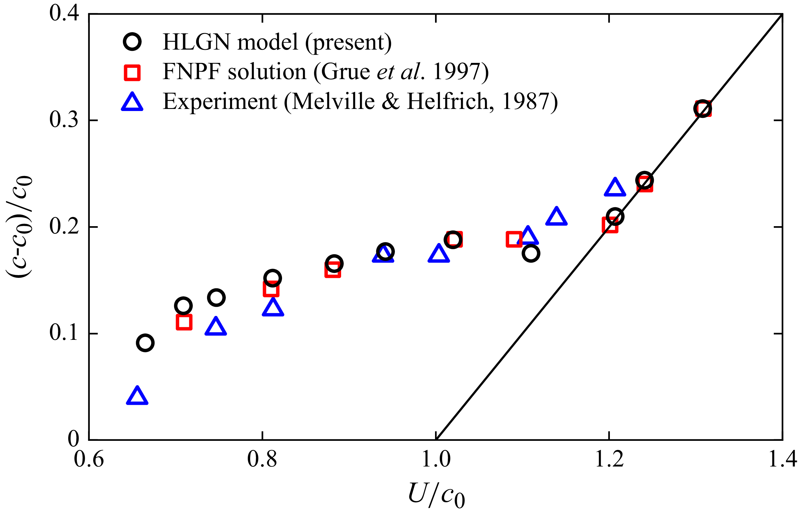
Relationships between the moving body speed and the excess speed of the generated internal wave, $\rho _1/\rho _2=0.8114$ and $H_1/H_2=1/4$ (the solid line marks where the generated internal wave has the same speed as the body).

The relationship between the excess speed $(c-c_{0})/c_{0}$ and the moving speed $U/c_{0}$ is shown in figure 7, comparing the results from the HLGN model, FNPF solution obtained by Grue et al. (Reference Grue, Friis, Palm and Rusas1997) and laboratory observations obtained by Melville & Helfrich (Reference Melville and Helfrich1987). The wave speed was determined in the laboratory by recording the moving time of the leading disturbance between the two recording stations located at 5 and 9.25 m. The results obtained from the HLGN model and FNPF solution followed the same procedure in extracting wave speed from the computations, with excellent agreement. Moreover, it can be observed that when the moving speed is greater than $U/c_{0}=1.2$ , the wave speed becomes identical to the moving speed of the body.

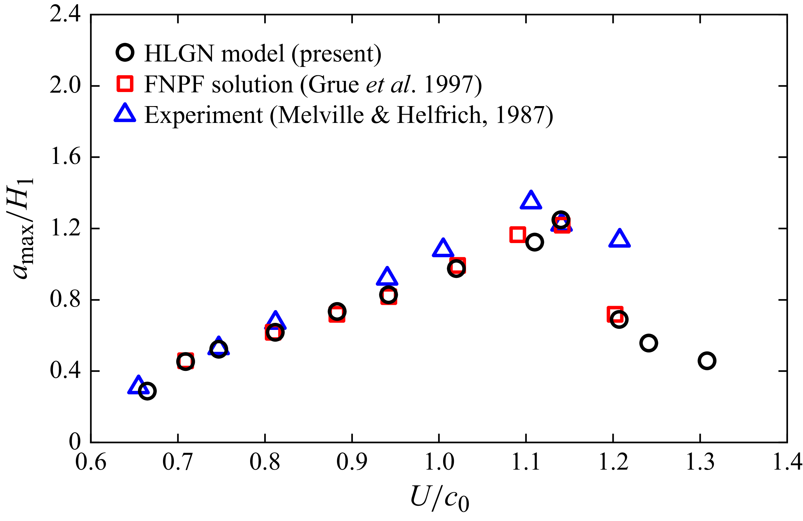
For the relationship between the moving speed of the body $U/c_{0}$ and the maximum wave amplitude $a_{max}/H_{1}$ as shown in figure 8, the HLGN model results are also compared with the results from the Euler solution obtained by Grue et al. (Reference Grue, Friis, Palm and Rusas1997) and laboratory observations obtained by Melville & Helfrich (Reference Melville and Helfrich1987). Grue et al. (Reference Grue, Friis, Palm and Rusas1997) presented the wave amplitude at the far end of the tank as the maximum amplitude. A similar approach is adopted in our present study. The agreement between the HLGN model, FNPF solution and the experimental observations is generally good. When the moving speed is smaller than $U/c_{0}=1.2$ , the amplitude of the generated internal waves increases as the moving speed increases. It is important to note that we also use the HLGN model to calculate the maximum wave amplitude for moving speeds exceeding $U/c_{0}$ = 1.2. When the moving speed is larger than $U/c_{0}=1.2$ , the results indicate that with a larger moving speed, the amplitude of the generated internal waves decreases. A similar phenomenon was also observed by Zhao et al. (Reference Zhao, Zhang, Duan, Wang, Guo, Hayatdavoodi and Ertekin2023a ) in the study on the generation of internal waves by bottom disturbance. Next, we focus on studying this phenomenon in more detail.

Figure 8.

Relationships between the moving body speed and the maximum amplitude of the generated internal wave, $\rho _1/\rho _2=0.8114$ and $H_1/H_2=1/4$ .

Figure 9.

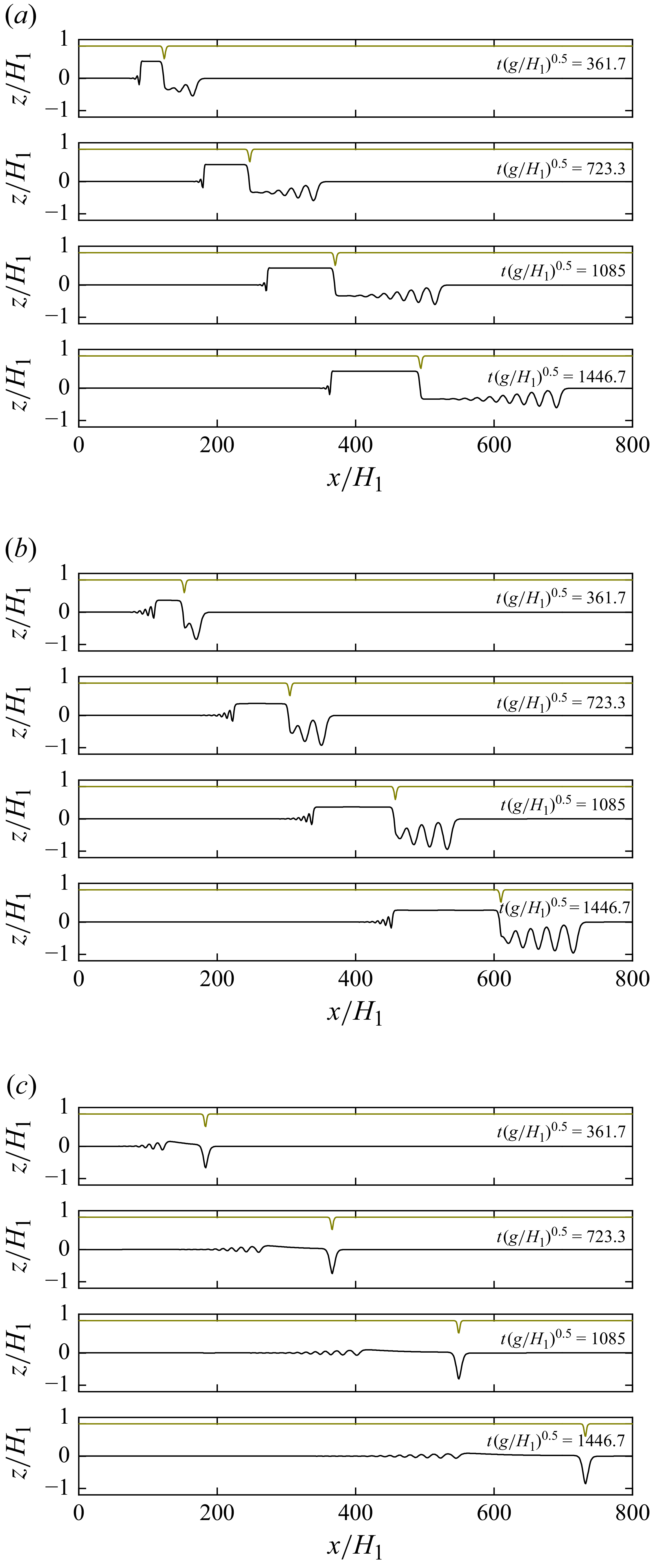
Generated internal waves at different moments with different moving speed, $\rho _1/\rho _2=0.8114$ and $H_1/H_2=1/4$ . Results are shown for (a) $U/c_{0}$ = 0.81, (b) $U/c_{0}$ = 1.0 and (c) $U/c_{0}$ = 1.2.

To further analyse the evolution of the internal wave generated by the moving surface disturbance, we compare the results obtained for different values of $U/c_0$ . Figure 9 illustrates wave profiles at four different moments (corresponding to the dimensional time of 20, 40, 60 and 80 s) under different moving speeds.

In figure 9, when the moving speed is $U/c_{0}$ = 0.81, the generated internal waves take the form of an undular bore, which is largely linear and, therefore, dispersive. As the speed increases to $U/c_{0}$ = 1.0, the waves develop into a sequence of ISWs, indicating enhanced nonlinearity. When the moving speed reaches $U/c_{0}$ = 1.2, a single soliton-like internal wave is produced, remaining aligned with the moving body and forming a locally steady supercritical solution. This transition from a dispersive undular bore to solitary internal waves occurs as the body speed increases and nonlinearity gradually strengthens, thereby suppressing dispersion. The observed behaviour is consistent with previous theoretical descriptions (Melville & Helfrich Reference Melville and Helfrich1987; Grue et al. Reference Grue, Friis, Palm and Rusas1997).

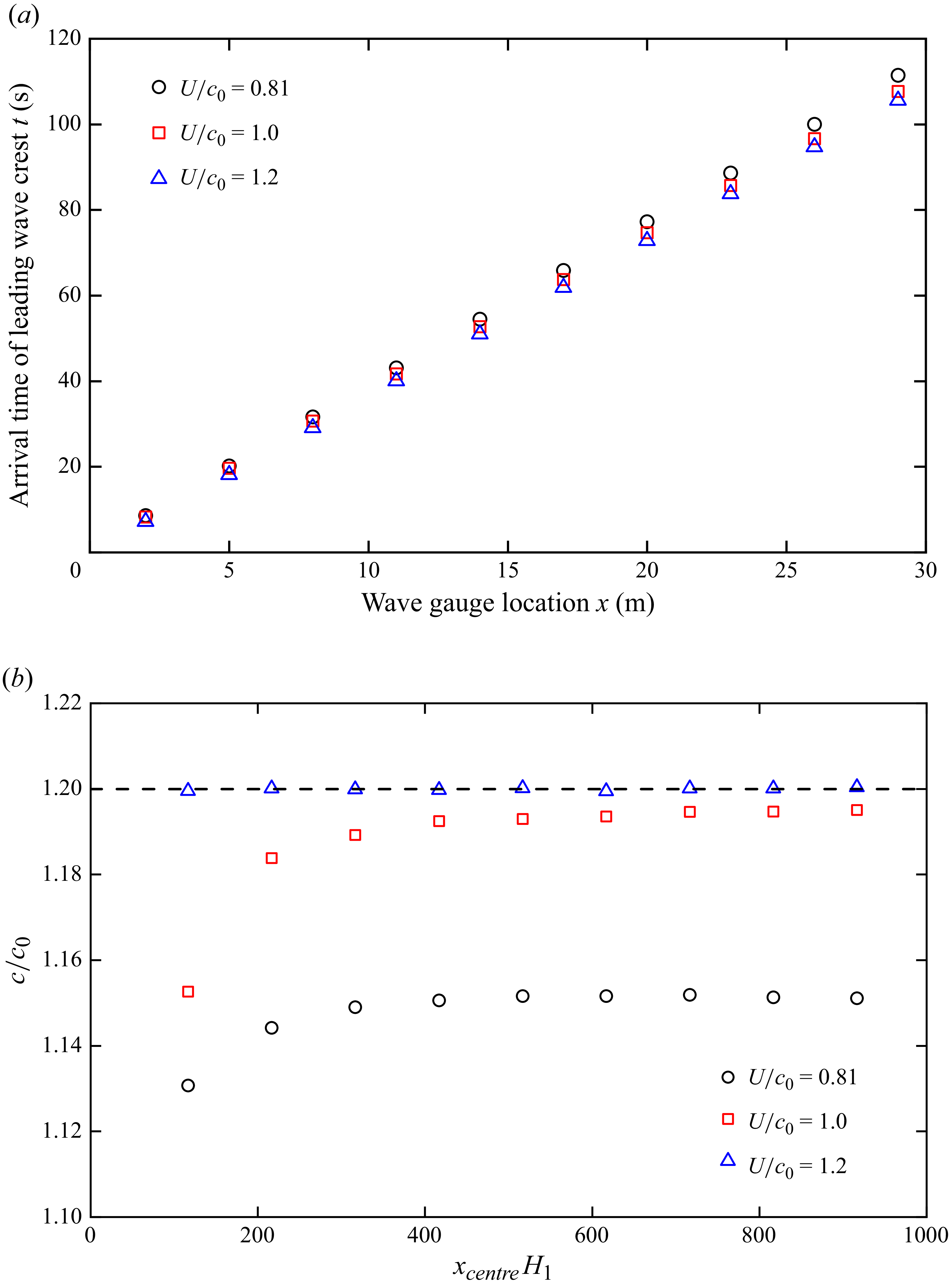
For the speed of the generated internal waves, figure 7 presents the relationship between the wave speed and the moving speed. However, since only two wave gauges were deployed in the experiment, it is difficult to capture the evolution of the internal-wave speed. To investigate the speed of the generated internal waves, numerical simulations were conducted in which 10 wave gauges were arranged in the numerical wave tank. These gauges were positioned at distances ranging from 2 to 29 m from the centre of the moving body, with a uniform spacing of 3 m.

Figure 10.

(a) Arrival times of leading wave crests at different gauges. (b) Internal-wave speed (the dashed line marks the moving speed of $U/c_{0}=1.2$ ). Evolution of the generated internal-wave speed with a different moving speed, $\rho _1/\rho _2=0.8114$ and $H_1/H_2=1/4$ .

Figure 10(a) shows the arrival times of the leading wave crests at different gauge locations. Based on these arrival times, the speeds of the leading wave were calculated between adjacent wave gauges, as shown in figure 10(b). Note that since the calculated wave speed represents the average speed between adjacent wave gauges, the horizontal coordinate ${{x_{\textit{centre}}}}/{{H_1}}$ in figure 10(b) corresponds to the midpoint between these gauges.

As shown in figure 10(b), when the moving speeds are $U/c_{0}$ = 0.81 and $U/c_{0}$ = 1.0, the wave speed of the generated internal waves initially increases and then approaches a steady value. At $U/c_{0}$ = 1.2, the internal-wave speed is consistent with the moving speed. This indicates that dispersion dominates at lower speeds, while nonlinearity becomes stronger at higher speeds, yielding a stable soliton-like propagation speed. In addition, the wave speed reaches the stable regime after the moving body has travelled about $x/H_{1}=500$ , corresponding to 15 m under the experimental conditions of Melville & Helfrich (Reference Melville and Helfrich1987). However, in their experiments the wave gauges were placed at 5 and 9.25 m, where the internal-wave speed had not yet stabilised. As a result, the wave speed calculated in figure 7 is lower than the fully developed wave speed. For instance, at $U/c_{0}$ = 1.0, the experimentally measured wave speed is $U/c_{0}$ = 1.17, which is lower than the fully developed wave speed of $U/c_{0}$ = 1.19.

4.4. Internal waves generated by a moving disturbance in linear shear current

In this subsection we investigate the effect of background shear current on internal waves generated by a moving body on the bottom, which goes beyond the capabilities of applications based on potential flow (e.g. Grue et al. Reference Grue, Friis, Palm and Rusas1997). To investigate the influence of vorticity, the background linear shear current is prescribed in the form

(4.1) \begin{align} {U_c}\left ( z \right ) = \omega z, \end{align}

which corresponds to a uniform vorticity $\omega$ . In the HLGN model, the effect of background shear current is incorporated through far-field boundary conditions. For the linear shear current, the boundary conditions as $x \to \infty$ are

(4.2) \begin{align} \eta = 0,\;\;\;\;\;\;\;\;\;\;{u_i}\left ( {x,z,t} \right ) = \sum \limits _{n = 0}^{{K_i-1}} {{u_{n,i}}\left ( {x,t} \right ){z^n}=\omega z},\quad(i=1,2). \end{align}

Since (3.2) involves integration along the $x$ direction, it is also necessary to introduce a far-field boundary condition. Under the linear background shear current, $u_{0,1}$ can be expressed as

(4.3) \begin{align} {u_{0,1}} & = \frac {1}{{{H_1} - \eta }} \nonumber \\& \quad \! \left [ \! {\frac {{\omega \left ( {H_1^2 - H_2^2} \right )}}{2} + \int _{ - \infty }^{ + \infty } {\frac {{\partial {h_2}}}{{\partial t}}{\textrm {d}}x} - \sum \limits _{n = 1}^{{K_2}} {\frac {{{\eta ^n} - h_2^n}}{n}{u_{n - 1,2}} - \sum \limits _{n = 2}^{{K_1}} {\frac {{H_1^n - {\eta ^n}}}{n}{u_{n - 1,1}}} } } \! \right ]\!, \end{align}

where $H_{1}$ and $H_{2}$ are the undisturbed thickness of the upper and lower layer, respectively.

The same bottom-moving semi-elliptical body as in § 4.2 is considered, moving at a constant non-dimensional speed $U=1.1c_{0}$ . The depth ratio and density ratio between the upper and lower layers are given as $H_1/H_2 = 4/1$ and $\rho _1/\rho _2 = 0.7873$ . Simulations are performed under various vorticity strengths from $S=-1$ to $S=1$ , where $S = {{\omega {H_1}} \mathord {\left / {\vphantom {{\omega {H_1}} {{c_0}}}} \right .} {{c_0}}}$ . Here, we adopt HLGN- $K_1-K_2$ with $K_1=K_2$ = 3. A sketch of the physical problem is shown in figure 11.

Figure 11.

Sketch of a body moving on the bottom with background shear current.

Figure 12 illustrates the elevation ISWs generated by a moving bottom disturbance under different vorticity strengths $S$ . The wave profiles shown correspond to the simulation results at $t(g/H_{2})^{0.5}$ = 1808. When $S$ is positive, increasing the vorticity strengths leads to narrower internal waves, and more solitary waves are generated within the same time interval. In contrast, when $S$ is negative, stronger vorticity produces broader waveforms and fewer solitary waves within the same duration.

This phenomenon arises from the modulation of the internal waves by the linear background shear. For an elevation solitary wave, the induced horizontal particle velocity is negative in the upper layer (opposite to the propagating direction of the wave) and positive in the lower layer (aligned with the propagating direction of the wave). With positive $S$ , the linear shear current is positive in the upper layer and negative in the lower layer, i.e. opposite to the wave-induced velocity in both layers (counter-flow). This opposition narrows the wave profile, increases the phase speed and allows more solitary waves to be generated over the same time. Conversely, for negative $S$ , the background shear current aligns with the wave-induced velocities (co-flow), which broadens the solitary wave, reduces the phase speed and results in fewer solitary waves. This finding is consistent with the steady solutions of ISWs in linear shear currents reported by Choi (Reference Choi2006) and Zhao et al. (Reference Zhao, Zhang, Duan, Wang, Hayatdavoodi and Ertekin2023b ).

Figure 12.

(a) Positive vorticity. (b) Negative vorticity. Internal-wave profiles with different vorticity strengths at $t(g/H_{2})^{0.5}$ = 1808, $\rho _1/\rho _2 = 0.7873$ , $H_1/H_2 = 4/1$ and $U=1.1c_{0}$ .

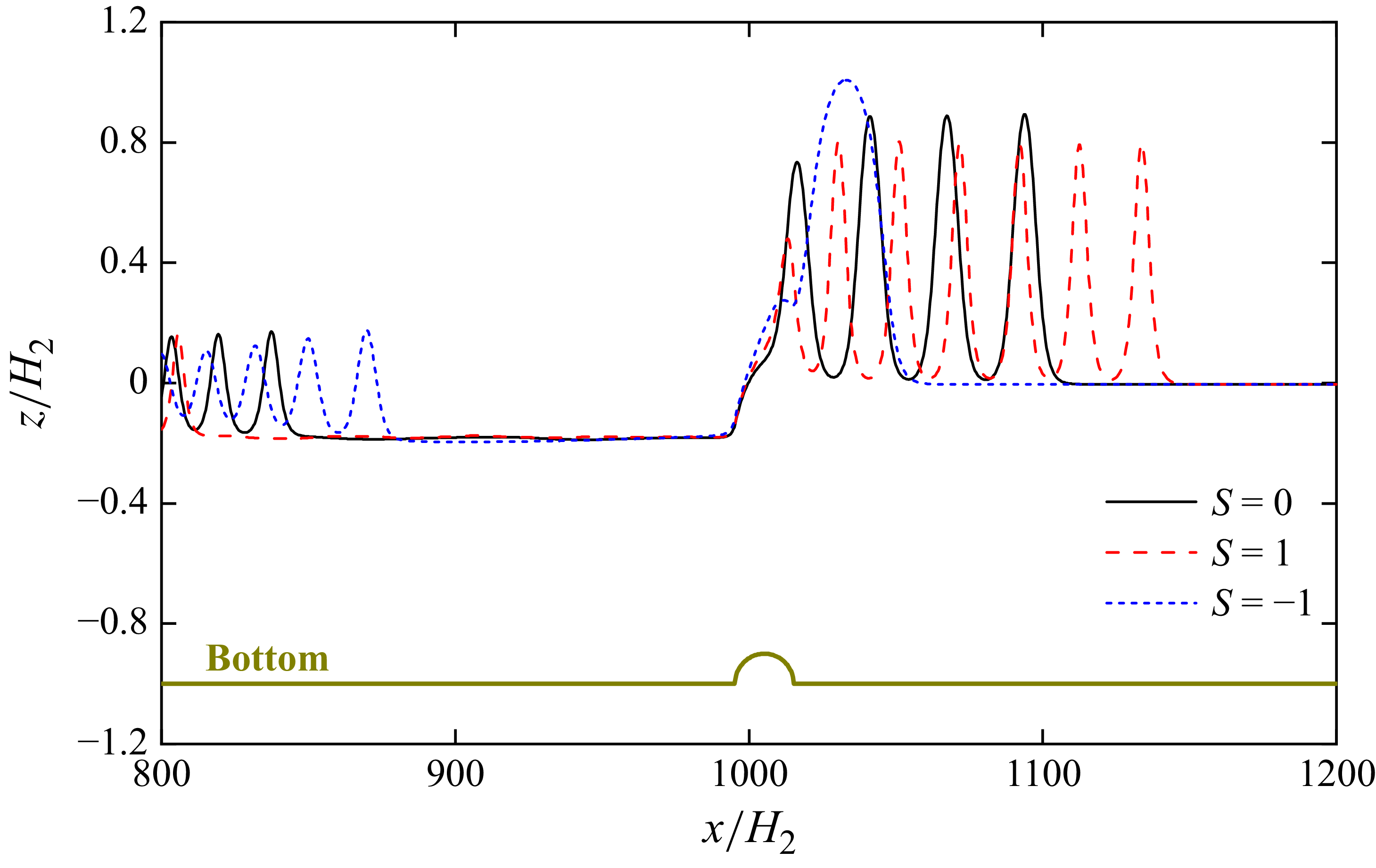
Figure 13 shows the wave profiles of ISWs generated by a moving bottom disturbance at $t(g/H_{2})^{0.5}$ = 1808 for $S=0$ , 1 and −1. Compared with the case of zero vorticity, when $S=1$ (counter-flow), the solitary waves become narrower with reduced amplitude. In contrast, when $S=-1$ (co-flow), the waves become broader and exhibit larger amplitudes. The variation in wave width is consistent with the steady solutions of ISWs in linear shear currents reported by Choi (Reference Choi2006) and Xu & Stastna (Reference Xu and Stastna2019). However, the amplitude behaviour observed here is opposite to their steady results. In the analyses by Choi (Reference Choi2006) and Xu & Stastna (Reference Xu and Stastna2019), co-flow broadens the wave but reduces its amplitude, whereas counter-flow narrows the wave and increases its amplitude. The discrepancy arises because, in the present study, ISWs are generated by a moving bottom body. Vorticity directly modifies the propagation speed of the generated waves: under counter-flow, the phase speed increases, so the solitary waves move away from the body more rapidly, reducing the effective forcing duration and resulting in smaller amplitudes. Conversely, under co-flow the phase speed decreases, so each solitary wave remains longer in the generation region, receives more energy input, and thus, attains a larger amplitude.

Figure 13.

Comparison of the internal-wave profiles with different vorticity strengths, $\rho _1/\rho _2 = 0.7873$ , $H_1/H_2 = 4/1$ and $U=1.1c_{0}$ .

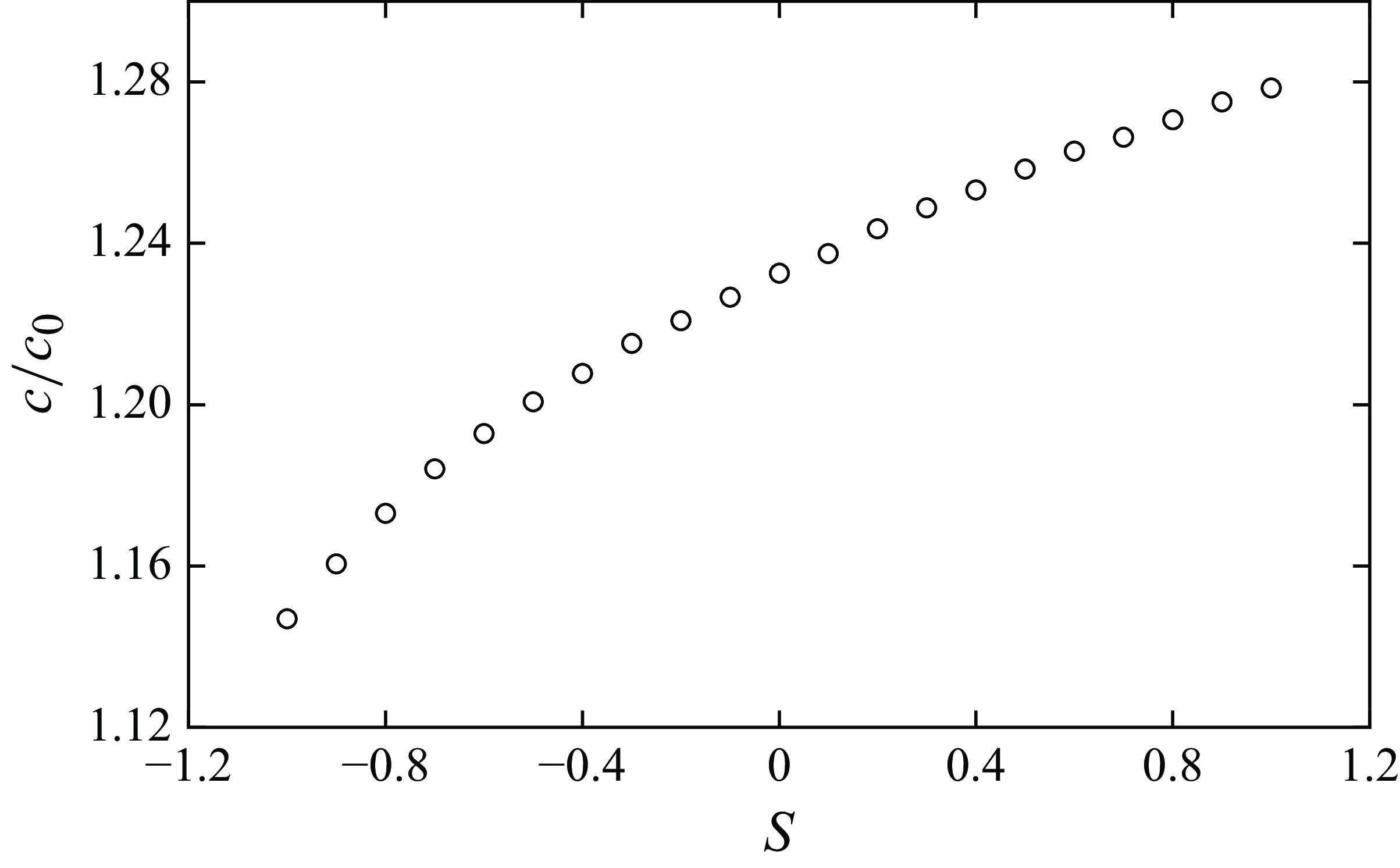
Figure 14 shows the relationship between the vorticity strength $S$ and the wave speed of the generated ISWs, where the wave speed was obtained from the displacement of the first crest between $t(g/H_{2})^{0.5}$ = 940 and 1808. From $S=-1$ to 0, the relationship between vorticity strength and wave speed is nonlinear, whereas from $S=0$ to 1, it is nearly linear. In this case, the modulation of the generated ISWs is more pronounced under negative vorticity.

Figure 14.

Relationship between the vorticity and the wave speed, $\rho _1/\rho _2 = 0.7873$ , $H_1/H_2 = 4/1$ and $U=1.1c_{0}$ .

Figure 15.

Velocity fields of generated internal waves with different vorticity strengths, $\rho _1/\rho _2 = 0.7873$ , $H_1/H_2 = 4/1$ and $U=1.1c_{0}.$ Results are shown for (a) $S=0$ , (b) $S=-1$ and (c) $S=1$ .

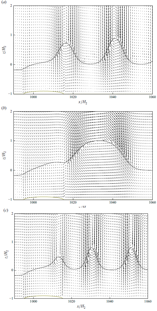
Figure 15 shows the velocity field of the ISWs generated by a moving body proceeding with different vorticity strengths. At the leading edge of the moving body, a distinct upward velocity lifts the interface and initiates the ISWs. Under no shear ( $S=0$ ), a clear anticlockwise recirculation cell forms under the crest, with vectors tilting upward on the right side (down wave) and downward on the left side (up wave) of the crest (see figure 15 a). With a co-flow ( $S=-1$ ), the cell is stretched streamwise, becoming flatter and wider; the core flow exhibits greater horizontal alignment and the crest becomes broader. Under a counter-flow ( $S=1$ ), the linear shear produces a pronounced modification of the fluid–particle horizontal velocity, and a secondary clockwise recirculation cell emerges between adjacent ISWs, yielding a more complex shear-recirculation structure. Overall, it is observed that the background shear current systematically modulates the ISWs velocity field by redistributing layerwise momentum and reshaping the closed-streamline morphology within the wave core.

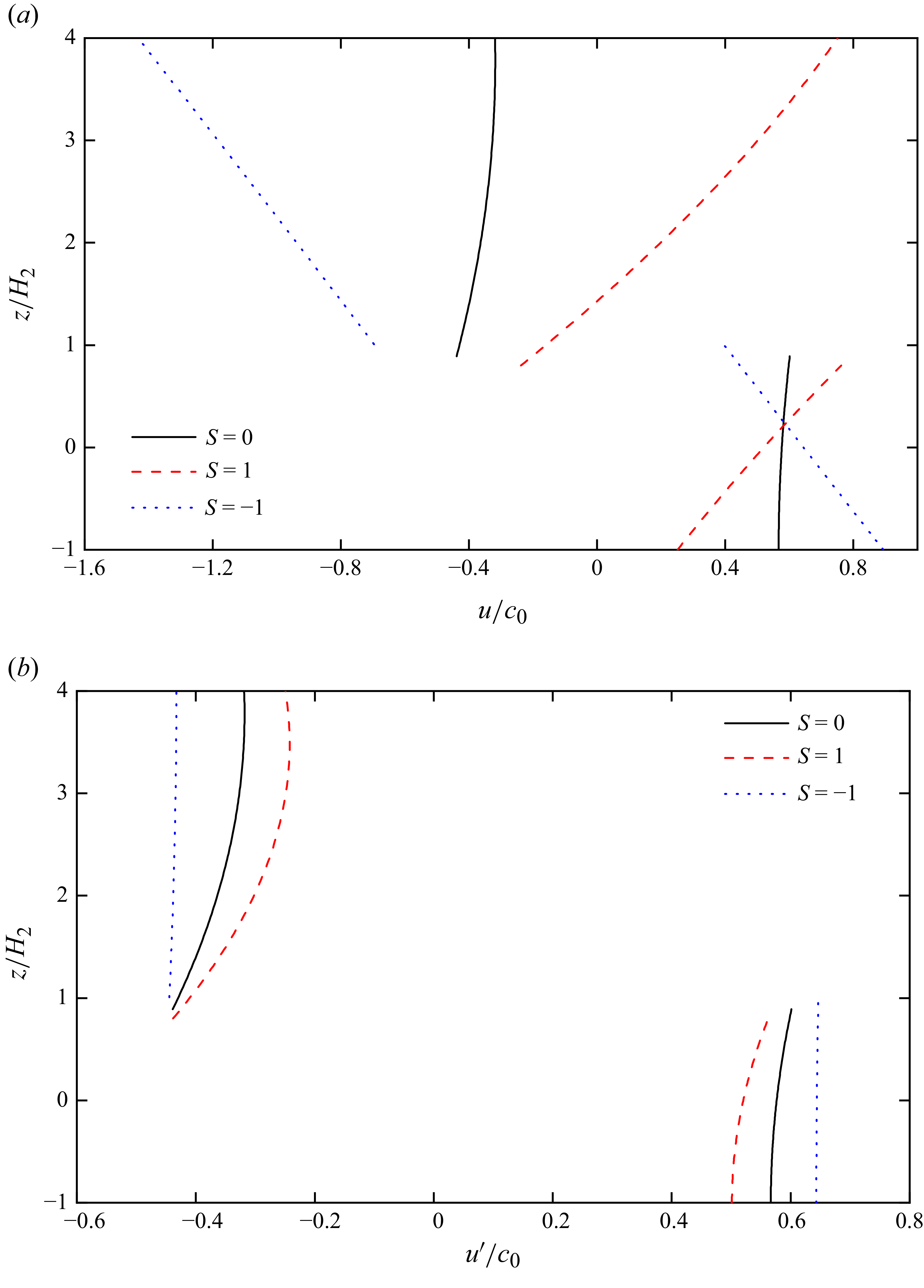
Figure 16 compares the horizontal velocity along the fluid column at the maximal displacement of the leading wave. With the background shear current included, as shown in figure 16(a), the large shear strength renders $u/c_{0}$ approximately linear with depth, so the curves mainly reflect the linear background profile rather than the wave-induced structure. After removing the background shear current ( $u'= u - {U_c}$ ) in figure 16(b), the fluid–particle horizontal velocity $ | {u'} |$ increases in the co-flow ( $S=-1$ ), whereas it decreases in the counter-flow ( $S=1$ ). Under co-flow, the vertical profiles of horizontal velocity are closer to linear with depth, while counter-flow produces profiles with noticeably greater curvature. The differences demonstrate nonlinear coupling between shear current and the wave, which modulates the crestwise velocity amplitude and its vertical structure.

Figure 16.

(a) Background shear current included. (b) Background shear current removed ( $u'= u - {U_c}$ ). Comparison of the horizontal velocity along the fluid column at the maximal displacement with different vorticity strengths, $\rho _1/\rho _2 = 0.7873$ , $H_1/H_2 = 4/1$ and $U=1.1c_{0}$ .

It should be noted that a uniformly moving body can be treated as equivalent to a uniform background current in the opposite direction, based on the principle of relative motion. However, this equivalence only holds for constant-speed motion. For unsteady motion, where the body velocity varies with time (Zhao et al. Reference Zhao, Zhang, Duan, Wang, Guo, Hayatdavoodi and Ertekin2023a ), or for motion along a sloping boundary, the body cannot be simply represented by a uniform flow. The theoretical framework developed in this paper can also be extended to account for such cases, including non-uniform body motion and oblique motion along a slope.