1. Introduction
Spherical Couette flow refers to the fluid motion in the annular space between two concentric spheres, where one or both spheres rotate. The spherical Couette system serves as a fundamental model in fluid dynamics, providing insights into complex flow behaviours and serving as a basis for studying geophysical and astrophysical phenomena. A Couette flow involves a cylindrical geometry (Marcus Reference Marcus1984). However, the principles have been extended to spherical polar geometries, resulting in a rich field of study with applications in geophysics, astrophysics and engineering. Spherical Couette flow provides a comprehensive and flexible framework for analysing fluid motion in spherical geometries (Nakabayashi & Tsuchida Reference Nakabayashi and Tsuchida1995). The interplay of rotation, viscosity and inertial effects in this configuration continues to inspire research and reveal intricate patterns of flow behaviour. It also serves as a model system for studying rotational instabilities (Wimmer Reference Wimmer1976), turbulence and angular momentum transport in various flow configurations (Mamun & Tuckerman Reference Mamun and Tuckerman1995; Rojas et al. Reference Rojas, Perevalov, Zürner and Lathrop2021). In this paper, we investigate the bifurcations leading to various flow topologies in the regime of a small gap between the inner and outer spheres.
Surface line integral convolution plotted over the azimuthal component of the vorticity contour with the axis marked by a dashed black line for sub-critical base flow at
 $Re=4500$
.

The investigations on the flow between two concentrically rotating spherical surfaces started in the early 1960s (Bratukhin Reference Bratukhin1961), where the stability of the flow was analysed by the method of small perturbations. Munson & Joseph (Reference Munson and Joseph1971) studied viscous flow between two coaxially rotating spheres and proposed a higher-order perturbation solution for large Reynolds number flows. A Legendre polynomial series expression was used for these large Reynolds number regimes. In a spherical Couette system, where only the inner sphere rotates, previous studies have extensively investigated both concentric and eccentric spherical annuli (Yuan et al. Reference Yuan, Fu and Ma1997), exploring the relative rotations of the spheres, including co-rotation and counter-rotation scenarios (Bassom & Soward Reference Bassom and Soward2004; Nakabayashi & Tsuchida Reference Nakabayashi and Tsuchida2005; Wicht Reference Wicht2014; Hoff & Harlander Reference Hoff and Harlander2019). Despite similarities to spherical Couette flow and Taylor Couette flows, secondary azimuthal flows add significant complexity to spherical Couette flows (Belyaev et al. Reference Belyaev, Monakhov and Yavorskaya1978). A distinctive feature of spherical Couette flow is the disappearance of Taylor vortices at higher Reynolds numbers, unlike Taylor–Couette flow (Bühler & Zierep Reference Bühler, Zierep, Comte-Bellot and Mathieu1987).
In the flow dynamics of a spherical Couette system with only the inner sphere rotating, the predominant factors influencing the flow are the gap ratio
 $(\beta )$
and the Reynolds number
 $(Re)$
(Junk & Egbers Reference Junk, Egbers, Egbers and Pfister2000; Hollerbach et al. Reference Hollerbach, Junk and Egbers2006), where the gap ratio is defined as the ratio of the gap to the radius of the inner sphere,
 $\beta =(R_o-R_i)/R_i$
, with the Reynolds number conventionally defined as
 $Re=R_i^2 \omega _{in}/\nu$
, where
 $\omega$
represents angular velocity and
 $\nu$
represents kinematic viscosity. When the gap ratio is small, the flow resembles Taylor–Couette flow with Taylor vortex cells near the equator for Re above the critical value (Tuckerman & Marcus Reference Tuckerman and Marcus2008). For a narrow gap and a Reynolds number greater than a critical value, a shift from the basic laminar flow state (Haberman Reference Haberman1962) to the first instability is observed in the form of Taylor vortices (Wimmer Reference Wimmer1981). Taylor vortices in spherical Couette flow were first observed experimentally by Khlebutin (Reference Khlebutin1972). Bühler & Zierep (Reference Bühler, Zierep, Comte-Bellot and Mathieu1987) evaluated the influence of time-dependent shear waves on the vortex flow formation. Researchers have explored various Taylor vortex flow regimes observed in a narrow-gap ratio in detail in the literature (Nakabayashi Reference Nakabayashi1983; Soward & Jones Reference Soward and Jones1983; Nakabayashi & Tsuchida Reference Nakabayashi and Tsuchida1988; Sha & Nakabayashi Reference Sha and Nakabayashi2001; Nakabayashi et al. 2002; Wang & Li Reference Wang and Li2004; Abbas & Shah Reference Abbas and Shah2022).
In medium-sized flow fields, instabilities manifest through symmetry-breaking bifurcations (Schrauf Reference Schrauf1986; Zikanov Reference Zikanov1996). These instabilities disrupt the equatorial symmetry of the vortices, leading to transitions that are often accompanied by hysteresis (Schrauf Reference Schrauf1986). The resulting vortex patterns range from no-vortex states to multiple-vortex states, depending on the Reynolds number and gap ratio (
 $Re$
and
 $\beta$
), and can be either symmetric or asymmetric with respect to the equator (Bühler Reference Bühler1990). At low
 $Re$
, the flow is steady and axisymmetric, with the number of vortex pairs generally increasing with
 $Re$
, according to a correlation by Yavorskaya (Reference Yavorskaya1980). Unstable to wavy and spiral instabilities were observed for Reynolds numbers beyond a critical value (Abbas et al. Reference Abbas, Shah, Hussain and Hussain2021). The asymmetric branch typically originates from a pitchfork bifurcation (Mamun & Tuckerman Reference Mamun and Tuckerman1995). Wereley & Lueptow (Reference Wereley and Lueptow1998); Tuckerman & Marcus (Reference Tuckerman and Marcus2008) tried to measure the size of vortices and found that the adjacent vortex pairs grow and shrink in size in order to redistribute the angular velocity among the radial shells. Wimmer (Reference Wimmer1976) has observed 5 modes of Taylor–Gortler vortices and concludes that it can be achieved by different routes with different initial conditions. We have used a similar strategy to obtain various branches of the bifurcation curve in the narrow-gap ratio in the present work.
In wide-gap ratios, however, the transition is direct to chaotic flow without the existence of Taylor vortices (Munson & Menguturk Reference Munson and Menguturk1975). Reverse Hopf bifurcation has also been observed that leads to re-laminarisation of the flow field (Nakabayashi et al. Reference Nakabayashi, Sha and Tsuchida2005). Hollerbach et al. (Reference Hollerbach, Junk and Egbers2006) have explored a wide range of aspect ratios
 $(0.1 \leqslant \eta \leqslant 10)$
and instability modes, including azimuthal waves for different wavenumbers (m), and their supercritical behaviour. Their findings emphasised the complexity of the flow, highlighting the presence of secondary bifurcations and time-dependent behaviours. The formation of complex vortical structures at higher Reynolds numbers is reported in detail in Nakabayashi & Yoichi (Reference Nakabayashi and Yoichi1988); Abbas et al. (Reference Abbas, Yuan and Shah2018); Abbas (Reference Abbas2023). Studies indicate that the axisymmetric state can become unstable at certain Reynolds numbers, resulting in the bifurcation of spiral states with varying wavenumbers. Understanding these bifurcations is vital for predicting flow behaviour in applications such as rotating machinery and geophysical flows (Mahloul et al. Reference Mahloul, Mahamdia and Kristiawan2016).
More recent studies have focused on the specific characteristics of medium and wide-gap spherical Couette flows. Goto et al. (Reference Goto, Itano, Sugihara-Seki and Adachi2021) investigated the bifurcation aspects of wide-gap spherical Couette flow, emphasising polygonal coherence and wavenumbers observed over transitional Reynolds numbers. The bi-stable behaviour and significant transitions in spherical Couette flow have been observed by Zimmerman et al. (Reference Zimmerman, Triana and Lathrop2011). The formation and destruction of zonal flow transport barriers and the presence of strong waves are highlighted in the paper, offering new insights into turbulent multiple stability. Meridional circulation, like differential rotation, is also noted to be an important factor in the spherical Couette flow (Pearson Reference Pearson1967).
The present work aims to understand the bifurcation characteristics and the flow topology for narrow-gap spherical Couette flow. This study is limited to the concentric spheres, with only the inner sphere rotating. The gap ratio is kept fixed at
 $\beta =0.24$
for this investigation, which is considered a narrow-gap ratio. Nakabayashi (2002) divided the current gap ratio of
 $\beta = 0.24$
in the medium-gap regime. However, later works, namely Inagaki et al. (Reference Inagaki, Itano and Sugihara-Seki2019), have re-evaluated this classification based on the underlying transition mechanisms. According to their findings,
 $\beta = 0.24$
exhibits transition characteristics consistent with the narrow-gap regime, where the onset of instability is driven by axisymmetric Taylor vortices, similar to those observed in cylindrical Taylor–Couette flow. In contrast, transitions in medium- and wide-gap regions are characterised by the breakdown of polygonal secondary waves at relatively high rotation rates, without the presence of Taylor vortices. Given that the primary focus of this study is on flow topology, we have adopted the classification of
 $\beta = 0.24$
as part of the narrow-gap regime to align with the observed transition dynamics and the framework established in the more recent literature. The governing equations and the numerical strategy, along with the validation and grid dependence study, are presented in § 2. We present a set of simulations for a wide range of Reynolds numbers. Simulations are run for three different initial conditions to obtain various branches of the bifurcation curve. Details of these simulations are presented in § 3. The topology and the dynamics of the flow on each branch of the bifurcation curve are discussed in § 4. Further discussions on the flow topology and instability are presented in § 5 and the phase space dynamics of the flow is explored in § 6. Finally, the discussion is concluded in § 7.
2. Simulation framework
2.1. Governing equations
The flow is governed by the non-dimensional continuity and incompressible Navier–Stokes equation
 \begin{align} \nabla \cdot \textbf {u} &=0, \end{align}
 \begin{align} \frac {\partial \textbf {u}}{\partial t} +\textbf {u}\cdot \nabla \textbf {u} &= -\nabla p + \frac {1}{{\textit {Re}}} \nabla ^2 \textbf {u}, \end{align}
where
 $\textbf {u}$
is the velocity vector and
 $p$
is the pressure. In the present study, the inner sphere is rotating at constant angular velocity (
 $\omega _i$
) while the outer sphere is held stationary. The natural choice of length scale and velocity scale are
 $R_i$
and
 $R_i\omega _i$
, respectively, where
 $R_i$
is the radius of the inner sphere. The parameter
 $\nu$
is the kinematic viscosity of the fluid. The Reynolds number (
 $Re$
) is defined as
 $Re=R_i^2\omega _i/\nu$
. The governing equations in spherical coordinates, where the velocity vector
 $\textbf {u}=(u_\phi$
,
 $u_\theta$
,
 $u_r)$
, are solved using Dedalus, a Python-based framework for solving partial differential equations using spectral methods.
The boundary conditions are:
(i) at the inner sphere,
 $r=R_i$
 \begin{align} u_{\theta }=u_r=0 \quad and \quad u_{\phi }=1 ;\end{align}
(ii) at the outer sphere,
 $r=R_o/R_i$
 \begin{align} u_{\theta }=u_r=u_{\phi }=0 .\end{align}
2.2. Spectral Direct Numerical Simulation using Dedalus
Equations (2.1) and (2.2) are solved in spherical coordinates using an open-source package Dedalus (Burns et al. Reference Burns, Vasil, Oishi, Lecoanet and Brown2020). It is a Python package to solve partial differential equations using a sparse spectral method. The use of spherical bases with a symbolic interface allows us to set up the problem and the governing equations. Dedalus is parallelised to run on large clusters. The domain is decomposed using pencil decomposition, and an in-built message passing interface parallelisation is used for the communication between the nodes. Dedalus makes use of Jacobi polynomials to form the spherical bases (Vasil et al. Reference Vasil, Lecoanet, Burns, Oishi and Brown2019; Lecoanet et al. Reference Lecoanet, Vasil, Burns, Brown and Oishi2019). The radial direction is discretised using Chebyshev polynomials. Dedalus implements the non-periodic boundary conditions using a modified tau-method (Clenshaw Reference Clenshaw1957). The equations are integrated in time using a third-order, four-step, implicit-explicit RungeKutta scheme. The simulations are run with a variable time-step size.
2.3. Grid dependence study and validation
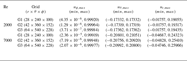
A grid independence study is performed for the simulations of a spherical annulus in spherical coordinates with the inner sphere rotating with different Reynolds numbers. The solutions for
 $ Re = 2000$
and
 $7000$
are obtained for three different grids, G1, G2 and G3, with varying divisions in the radial, polar and azimuthal directions. The maximum and minimum values of the azimuthal and radial components of the velocity field in the domain are compared for these three grids. Table 1 shows the grid dependency for both Reynolds numbers. The results are obtained for a variable time step between
 $10^{-2}$
and
 $10^{-4}$
. The simulations were run with an adaptive time-stepping algorithm to ensure numerical stability and accuracy. The exact time-step size varied depending on the Reynolds number and flow condition, with a smaller time-step size used for higher Reynolds numbers or flow states with higher vorticity. For example at
 $Re =6300$
the time step is
 $5.58\times 10^{-3}$
. The differences in the maximum and minimum values for the G2 and G3 grids are within 5% for both the Reynolds numbers. Therefore, G2 is chosen as the optimal grid for all the simulations presented in this study.
Grid dependence study for
 $\beta$
= 0.24 for
 $Re = 2000$
and
 $7000$
. Maximum and minimum contour values in the domain have been compared for three different grids for the azimuthal and radial components of the velocity.

Visualised flow pattern of five spiral waves from (a) Wulf et al. (Reference Wulf, Egbers and Rath1999) and (b) the azimuthal component of the vorticity calculated using the present numerical model for a gap ratio of
 $\beta =0.5$
and
 $Re=1320$
.

The results from the present computations are validated qualitatively as well as quantitatively with the existing literature for a range of Reynolds numbers, gap ratios and rotation rates. Figure 2 shows the azimuthal component of the vorticity from the present study for a gap ratio of
 $0.5$
and
 $Re=1320$
. The results are compared with the flow visualisation of experimental results from Wulf et al. (Reference Wulf, Egbers and Rath1999), who observed a periodic supercritical flow of wavenumber
 $k=5$
. While Wulf et al. (Reference Wulf, Egbers and Rath1999) provides experimental evidence, Abbas et al. (Reference Abbas, Yuan and Shah2018) has numerically observed
 $k=5$
spiral waves for
 $Re=1280$
using an artificial compressibility method. The present study reproduces the same flow pattern and vorticity distribution as Wulf et al. (Reference Wulf, Egbers and Rath1999), confirming the validity of the proposed numerical method.
Comparison of the present azimuthal and radial components of velocity with the results of Hollerbach et al. (Reference Hollerbach, Junk and Egbers2006) at (a)
 $Re=11270$
and
 $\beta =0.1$
and (b)
 $Re=489$
and
 $\beta =1$
.

Figure 3(a) shows the azimuthal and radial components of velocity at the equatorial plane along the radial direction for a gap ratio of
 $0.1$
and
 $Re=11270$
. The present study results are in perfect agreement with the results of Hollerbach et al. (Reference Hollerbach, Junk and Egbers2006), who used a finite difference method. The azimuthal velocity is higher than the radial velocity, indicating a strong shear layer near the inner sphere. Figure 3(b) shows the same components of velocity for a gap ratio of 1 and
 $Re=489$
. Again, the present study results match well with the results of Hollerbach et al. (Reference Hollerbach, Junk and Egbers2006). The azimuthal velocity is higher than the radial velocity, but the difference is smaller than in figure 3(a), indicating a weaker shear layer.
Comparison of flow structures in the
 $r-\theta$
plane for
 $\beta =0.14$
and
 $Re=1000$
; (a) azimuthal component of vorticity contour and (b) streamlines. For both plots, the left half is from Abbas et al. (2021) and the right half from the present simulations.

Further, figure 4 compares the streamlines and azimuthal component of the vorticity line contour for a steady two-vortex flow observed for a gap ratio of
 $0.14$
and
 $Re=1400$
. The present study results are consistent with the previous study by Abbas et al. (2021), who reported a similar flow structure and vorticity pattern using different numerical schemes. These comparisons demonstrate that the proposed numerical method can accurately simulate the spherical Couette flow with inner sphere rotation for different flow regimes and parameters. The results also agree well with the existing theoretical and experimental studies on the topic, validating the physical relevance and significance of the present study.
3. Details of simulations
Variation of radial velocity component,
 $\langle u_r\rangle _{\phi }$
, for various
 $Re$
. Axisymmetric represents the branch on which the flow remains axisymmetric up to the largest Reynolds number studied in the present study. TWI represents the branch on which the flow is dominated by the travelling wave instability. EI represents the branch dominated by equatorial instability. EI_Backward is the backward extension of the EI branch by reducing the Reynolds number of the flow on the EI branch, showing the hysteresis. The topology of the flow at different branches for various
 $Re$
is shown using contours of
 $\theta$
component of vorticity.

The present work analyses the flow for a range of Reynolds numbers
 $(400{-}6300)$
for a fixed gap ratio
 $\beta =0.24$
. Figure 5 shows a radial component of velocity,
 $u_r$
, averaged in the
 $\phi$
direction, plotted for a range of Reynolds numbers. This figure shows the bifurcations in spherical Couette flow for
 $\beta =0.24$
with
 $Re$
as a parameter. We have performed mainly three sets of simulations to obtain various branches of the bifurcation curve of the flow shown in figure 5. In the first set, all the simulations are initialised with the velocity field of the previous lower
 $Re$
simulation. Results of these simulations form branch I (upper branch) of figure 5 (black circles). Hereafter, this branch is referred to as the axisymmetric branch.
For the second set of simulations, all the simulations start with zero initial field and zero initial perturbation. The results of these simulations form branch II (middle branch) of figure 5 (blue crosses). This branch is referred to as the travelling wave instability (TWI) branch in the following discussions. For the third set, each simulation is started with the following perturbation (Yuan Reference Yuan2012):
 \begin{align} \hat {v}_r&=-4 \varepsilon _1 \frac {\left (r-R_i\right )\left (r-R_o\right )}{\left (R_o-R_i\right )^2} \cos \left [\pi \left \{1-\frac {R_m\left (\frac {\pi }{2}-\theta \right )}{\left (R_i-R_o\right )}-\varepsilon _2 \sin \left (m_a \phi \right )\right \}\right ], \end{align}
 \begin{align} \hat {v}_\theta &=\varepsilon _1 \sin \left [\frac {\pi }{2} \frac {\left (r-R_i\right )\left (r-R_m\right )\left (r-R_o\right )}{\left (R_o-R_i\right )^3}\right ] \nonumber \\ &\quad\times \sin \left [\pi \left \{1-\frac {R_m\left (\frac {\pi }{2}-\theta \right )}{\left (R_i-R_o\right )}-\varepsilon _2 \sin \left (m_a \phi \right )\right \} \frac {1}{\beta }\right ]. \end{align}
Here,
 $(\hat {\cdot })$
denotes the perturbation,
 $R_m = 0.5(R_i+R_o)$
is the mean radius,
 $\varepsilon _1$
is the amplitude of the perturbation velocities and
 $\varepsilon _2$
is the amplitude of the azimuthal perturbation. The values of the perturbations are chosen as
 $\varepsilon _1=10^{-4}$
,
 $\varepsilon _2 = 0.4$
and
 $m_a=6$
in accordance with the literature (Yuan Reference Yuan2012; Abbas et al. Reference Abbas, Yuan and Shah2018). This perturbation satisfies the no-slip boundary conditions at the inner and the outer spheres. A similar form of perturbation is used in Taylor–Couette flow and mimics the Taylor vortices (Schröder & Keller Reference Schröder and Keller1990). This branch is referred to as the equatorial instability (EI) branch.
All the three branches of the curve separate from each other approximately at
 $Re=4500$
. Once the first point of a new branch is obtained, the subsequent points on that particular branch are obtained using the axisymmetric branch’s strategy. In addition to these three sets of simulations, we have carried out simulations to extend the EI branch backward. The Reynolds number is reduced to check the backward extent (hysteresis) of the EI branch, until the flow jumps back to the axisymmetric branch. In the following sections, we describe the dynamics and topology of the flow on each branch as the Reynolds number is varied.
4. Results and discussion
4.1. Branch I: axisymmetric branch
As mentioned, each simulation on this branch starts from the velocity field of the previous Reynolds number with no superimposed perturbation. The flow for the lowest
 $Re$
is started from
 $Re=10$
, with zero initial velocity field. The value of
 $Re$
is increased with an increment in steps of
 $10$
using the previous case velocity field. At large
 $Re$
, the values are increased in steps of
 $250$
. Below
 $Re=430$
, the flow is in a steady state that has a circular cell in each hemisphere. This state is called the “zero-vortex” or “sub-critical” basic flow state (Abbas & Shah Reference Abbas and Shah2022). This base state is shown in figure 6 for
 $Re=300$
using vorticity lines in a
 $r$
–
 $\theta$
plane and the contours of azimuthal vorticity in side view and top view.
Basic state
 $Re=300$
, showing circular cell in both hemispheres; (a) azimuthal vorticity line contours in a
 $r-\theta$
plane, (b) contours of azimuthal vorticity in side view and (c) in top view.

Surface line integral convolution of vorticity, coloured with the azimuthal component of vorticity, for Reynolds numbers (a)
 $400$
, (b)
 $600$
, (c)
 $800$
and (d)
 $1000$
. The dashed curve shows the location of the zoomed-in portion in each figure to show the vortex pinching. (e) Streamlines showing the pinching in the
 $r-\theta$
plane for
 $Re = 600$
.

As the Reynolds number is increased further, the flow starts to pinch at the equator on each side of the hemisphere at
 $Re=430$
. An earlier study by Yavorskaya (Reference Yavorskaya1980) found a correlation between the gap ratio
 $(\beta )$
and the critical Reynolds number at which a zero-vortex flow with a pinch is first observed. This study verified that the correlation
 $Re_c = 41.3(1 + \beta )\beta ^{-\frac {3}{2}}$
is valid in the range
 $0.08\leqslant \beta \leqslant 0.25$
. According to this correlation, the critical Reynolds number for
 $\beta = 0.24$
is
 $Re_c=435.56$
. We have found the critical Reynolds number, where the pinching starts, to be
 $430$
in our computations. Additionally, Yavorskaya (Reference Yavorskaya1980) has identified a correlation for the maximum number of Taylor vortex pairs on each side of the hemisphere near the equator, which is given by
 $i = 0.21\beta ^{-\frac {4}{3}}$
. According to this correlation, for
 $\beta =0.24$
, we find
 $i=1.41$
, indicating the presence of a one-vortex flow. However, we do not see one-vortex flow in our study, which is also observed in a recent study (Abbas Reference Abbas2019) for similar values of the gap ratios. Figure 7 shows the surface line integral convolution plots of the vorticity, coloured by the azimuthal vorticity component. A portion of the sphere is cut to show the flow in the
 $r$
 $\theta$
plane. Dashed ellipses show the location of the zoomed-in portion of the flow in the vicinity of the equator. At
 $Re=400$
, there is no vortex, and the flow is similar to the base state with circular cells in both hemispheres (figures 7
a and 7
e). At
 $Re=600$
, we observe a pinching of the vortex at the equator (figure 7
b), which is also visible at
 $Re=800$
, as shown in figure 7(c). At
 $Re=1000$
, we observed that this pinching disappears and the flow returns to the two-cell flow, as shown in figure 7(d).
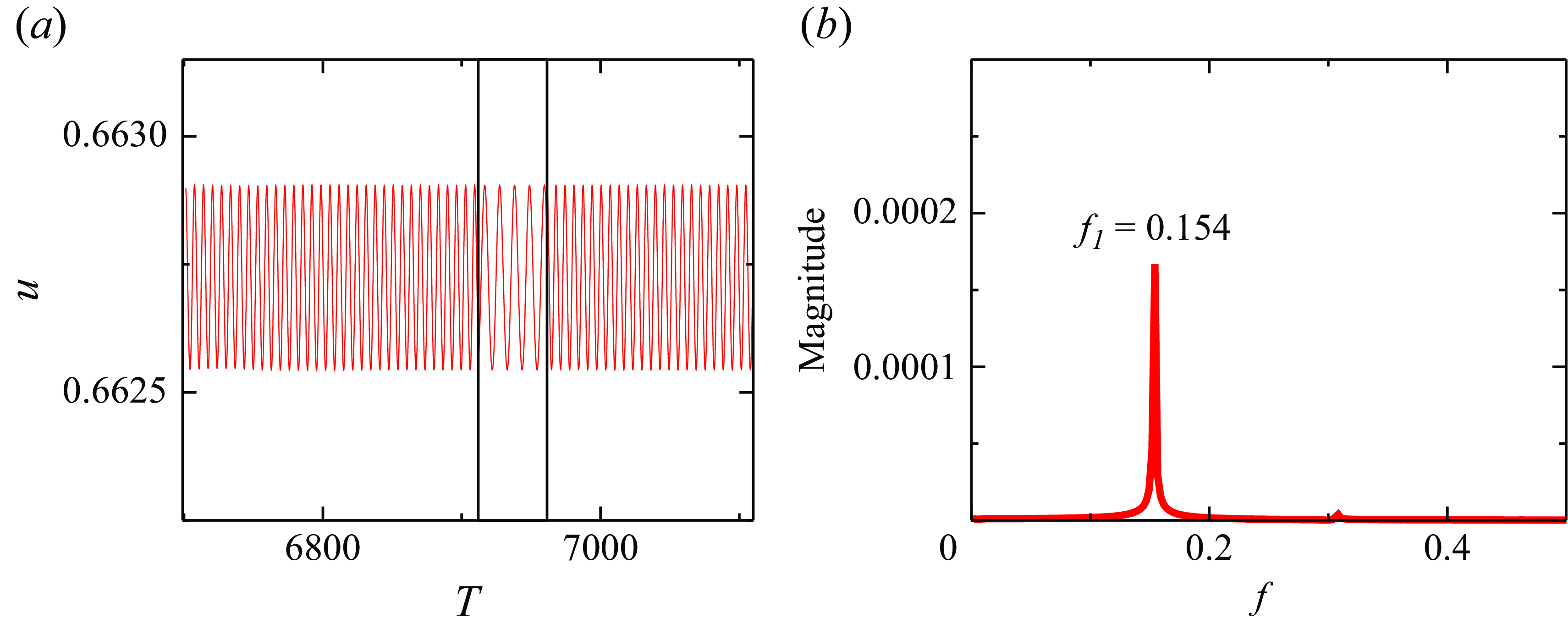
(a) Time series of the magnitude of the velocity and (b) corresponding DFT of timeseries data, probed at a point located at the mid-radius
 $(R_i+R_o)/2$
, close to the equator for
 $Re=6250$
(upper branch).

(a) Variation of
 $u_\phi$
along
 $\theta$
at a radius
 $r=(R_i+R_o)/2$
for various
 $Re$
on the axisymmetric branch. The profiles are averaged in the azimuthal direction. (b) Contours of
 $u_\phi$
along with velocity vectors at the mid-radius for
 $Re=6300$
on the axisymmetric branch at an instant. The white arrow shows the direction of the equatorial jet.

The flow remains steady for
 $Re\lt 6250$
. At
 $Re=6250$
, the flow becomes unsteady, and a weakly periodic state of the flow emerges. To analyse the nature of the flow, we placed a numerical probe at the mid-radius, close to the equator, at
 $\phi =0$
. Figure 8 shows the time history of the velocity magnitude obtained from this probe along with the discrete Fourier transform (DFT) of the signal. We observe that the flow is weakly periodic with a fundamental frequency of
 $f=0.154$
, which corresponds to a time period of
 $T\approx 6.5$
. Here, frequency (
 $f$
) is scaled with the rotating inner sphere frequency,
 $\Omega$
. We have not observed any non-axisymmetry up to
 $Re=6250$
, which is the largest Reynolds number analysed on the axisymmetric branch in the present study.
At the low Reynolds numbers, the flow shows an equatorial jet (at
 $\theta =\pi /2$
). Figure 9(a) shows the azimuthal velocity,
 $u_\phi$
at the mid-radius, averaged in the azimuthal direction, along
 $\theta$
. At the largest Reynolds number, slow-moving jets are also observed near the poles apart from the dominant equatorial jet. These jets can also be seen in figure 9(b), which shows the contours of
 $u_\phi$
at an instant along with the velocity vectors for
 $Re=6250$
. A white arrow at the equator illustrates the direction of the equatorial jet. Slow-moving jets are also visible near the poles. The following sub-sections discuss the other branches of the flow.
4.2. Branch II: travelling wave instability branch
Contours of azimuthal vorticity showing spiral wavy flow at
 $Re=4500$
on branch
 $II$
. (a) Side view, (b) top view and (c) iso-surface of
 $u_\phi =-0.0289$
. (d) Contours of azimuthal vorticity
 $\xi (\phi ,t)$
at
 $r=(R_i+R_o)/2$
,
 $\theta \approx 0$
is plotted along
 $\phi$
at
 $Re=4500$
. Yellow dashed lines show the direction of propagation of the wave.

The travelling wave instability branch (blue) separates from the axisymmetric branch approximately at
 $Re=4500$
as shown in figure 5. Once the first point of this branch is found
 $({\textit {Re}}=4500)$
, all the subsequent cases are initialised with the velocity field of the previous lower Reynolds number case. At
 $Re=4500$
, the flow loses its axisymmetry and supports a spiral instability of wavenumber,
 $k=7$
. Figure 10 shows a side view and a top view of azimuthal vorticity along with the iso-surface of
 $u_\phi = -0.0289$
to display the structure of the spiral instability. This spiral instability manifests itself in the form of a modulated travelling wave. This travelling wave is shown in figure 10(c), which shows the contours of azimuthal vorticity. Azimuthal vorticity
 $\xi (\phi ,t)$
is computed along the
 $\phi$
, at mid-radius
 $r=(R_i+R_o)/2$
and near the pole,
 $\theta \approx 0$
. Figure 10(c) plots this value at each time along
 $\phi$
, which clearly reveals the direction of propagation of the wave. The yellow dashed lines in the figure show the direction of propagation of this wave.
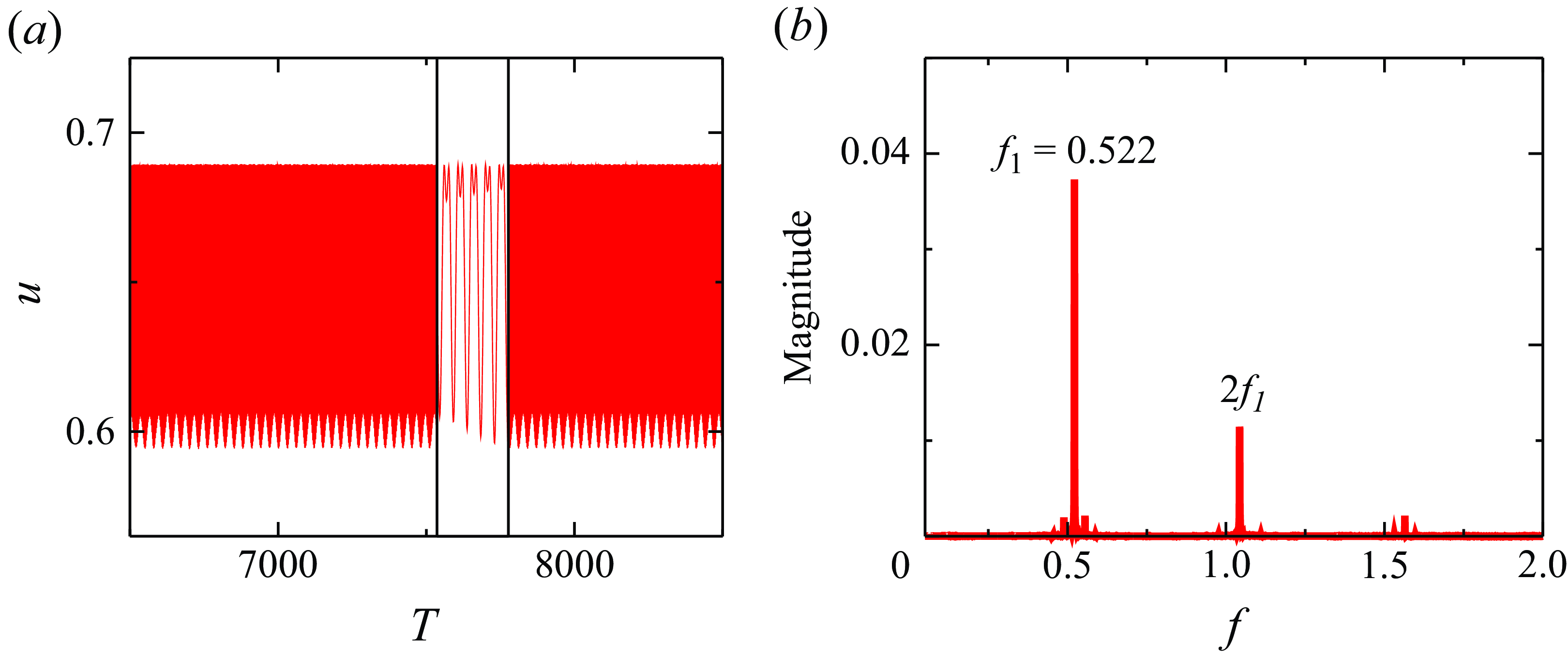
(a) Time series of the magnitude of the velocity and (b) corresponding DFT of timeseries data, probed at a point located at the mid-radius
 $(R_i+R_o)/2$
, close to the equator for
 $Re=4500$
.

To understand the dynamics of the flow, we placed a probe to measure the time history of the velocity at the mid-radius
 $(r=(R_i+R_o)/2)$
, near the equator, and at
 $\phi =0$
. The variation of the magnitude of the velocity,
 $u$
, at this location and the corresponding DFT of the signal, are shown in figure 11. The signal shows a fundamental frequency of
 $f=0.522$
, with its first harmonic. The fundamental frequency corresponds to a time period of
 $T\approx 1.92$
. As the Reynolds number is increased, the flow undergoes a direction-reversing bifurcation where the direction of propagation of the spiral wave is reversed. This transition starts approximately at
 $Re = 4700$
. Figure 12 shows the sequence of this transition using contours of the azimuthal vorticity (similar to that of the figure 10
c) along with frequencies supported by the flow for
 $Re=4700$
and
 $5100$
. The reversal of the propagation direction of the travelling wave is completed approximately at
 $Re\approx 5340$
, as shown in figure 13. During this transition, the fundamental frequency is increased slightly to
 $f\approx 0.594$
at
 $Re=4900$
and then returns back to
 $f\approx 0.522$
at
 $Re=5340$
when the transition is completed. This increase in the frequency also coincides with a local peak observed in the middle branch shown in the figure 5. The flow at
 $Re=5340$
also shows two new frequencies
 $f_1=0.376$
and
 $f_2=0.664$
and their harmonics, as shown in figure 14. The presence of the harmonics and the multiple frequencies indicate a period-doubling bifurcation and the chaotic state of the flow, respectively. These aspects of the flow are discussed in § 6.
The above-observed spiral instability is accompanied by an equatorial instability of wavenumber
 $k=7$
at
 $Re=4500$
which can be seen in figure 10(a). At larger Reynolds numbers, we have observed multiple wavenumbers in the equatorial instability, which are discussed in § 5 in detail. This equatorial instability is associated with an equatorial jet. Figure 15(a) shows the
 $\theta$
variation of the azimuthal velocity at a mid-radius, averaged in the azimuthal direction, for a range of Reynolds numbers. The figure shows a dominant equatorial jet similar to the axisymmetric branch. Figure 15(b) shows the contours of
 $u_\phi$
along with the velocity vectors at an instant for
 $Re=5360$
. We observe that, although the equatorial jet meanders due to the instability at a large Reynolds number, the flow still shows a strong mean equatorial jet. The jet becomes stronger during the direction reversal of the travelling wave, as is evident from figure 15(a). Figure 15 also shows instabilities in the jet profile near the polar region. Figure 16 shows the side views and the top views of the contours of azimuthal vorticity at an instant for a range of Reynolds numbers. This sequence shows that multiple azimuthal modes appear in the polar and equatorial regions (particularly figure 16
a) during the direction reversal of the travelling wave. This concurs with the appearance of the instabilities observed in the jet profile in figure 15(a). However, we have not confirmed reversal analytically/quantitatively. It can be seen that the spiral instability of
 $k=7$
, observed at
 $Re=4500$
(shown in figure 10
b) becomes unstable as the Reynolds number is increased, which gives rise to multiple azimuthal modes observed at higher
 $Re$
. It can also be noted that the spiral modes observed on this branch are spread throughout the domain, as opposed to the instability confined in the vicinity of the equator for EI branch, discussed in the following section. The spiral instability along with the equatorial instability are discussed further in § 5.
Contours of azimuthal vorticity
 $\xi (\phi ,t)$
at
 $r=(R_i+R_o)/2$
;
 $\theta \approx 0$
is plotted along
 $\phi$
and the DFT of timeseries data is also plotted, probed at a point located at the mid-radius
 $(R_i+R_o)/2$
, close to the equator, respectively for (a,b)
 $Re=4700$
and (c,d)
 $Re=5100$
. Dashed yellow lines in (a,c) show the direction of propagation of the wave.

Contours of azimuthal vorticity
 $\xi (\phi ,t)$
at
 $r=(R_i+R_o)/2$
;
 $\theta \approx 0$
is plotted along
 $\phi$
at
 $Re=5340$
. Yellow dashed lines show the direction of propagation of the wave.

(a) Time series of the magnitude of the velocity and (b) corresponding DFT of timeseries data, probed at
 $(R_i+R_o)/2$
at the equator for
 $Re=5340$
.

Variation of
 $u_\phi$
along
 $\theta$
at a radius
 $r=(R_i+R_o)/2$
for various
 $Re$
on the TWI branch. The profiles are averaged in the azimuthal direction. (b) Contours of
 $u_\phi$
along with velocity vectors at the mid-radius for
 $Re=5360$
on the TWI branch at an instant. The white arrow shows the direction of the mean flow of the equatorial jet.

Contours of azimuthal vorticity at an instant in side view and top view respectively for (a,e)
 $Re=4700$
, (b,f)
 $Re=4900$
, (c,g)
 $Re=5100$
and (d,h)
 $Re=5340$
.

4.3. Branch III: equator instability branch
The EI branch of the bifurcation curve shown in figure 5 also separates from the axisymmetric branch approximately at
 $Re=4500$
. Similar to the TWI branch, as soon as the first point of this branch is obtained, all the subsequent points on this branch are obtained by initialising the velocity field from the previous
 $Re$
case. Once on this branch, this flow field is also used to extend the branch backward by reducing
 $Re$
, shown by the green branch in figure 5. Due to the hysteresis, the flow does not jump to the axisymmetric branch (branch I) immediately upon reducing the
 $Re$
below a value of
 $4500$
. The backward branch can be continued to a very low Reynolds number of
 $Re=400$
, before the flow jumps back to the axisymmetric branch (cf. Figure 5).
Two-cell flow on the EI branch shown by contours of azimuthal vorticity from (a) to (d) for Reynolds numbers
 $4500, 4750, 5750$
and
 $6250$
respectively. Figures (e) to (h) show vortex lines in an
 $r-\theta$
plane for the respective Reynolds numbers.

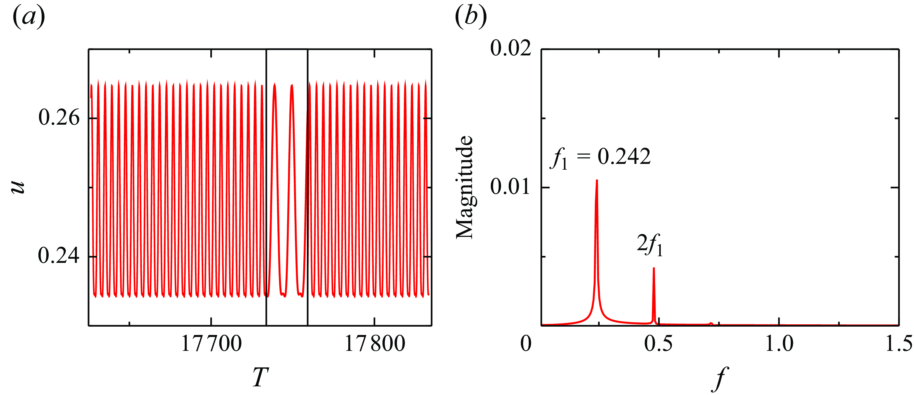
(a) Time series of the magnitude of the velocity and (b) corresponding DFT of timeseries data, probed at
 $(R_i+R_o)/2$
at the equator for
 $Re=4750$
on the EI branch.

Figures 17(a–d) show the contours of azimuthal velocity for
 $Re=4500$
to 6250 and figures 17(e–h) show the corresponding surface line integral convolution plots, coloured by the azimuthal vorticity, in the
 $r-\theta$
plane. In the forward bifurcation, at
 $Re\lt 4500$
, the flow is axisymmetric and exhibits a jet emanating radially outward from the inner sphere at the equator. At
 $Re=4500$
, while the flow is still axisymmetric, this radial jet hits the outer sphere, and the flow exhibits a two-vortex flow similar to the axisymmetric branch, as shown in figures 17(a) and 17(e). This radial jet is discussed in § 5. At Re = 4750, this radial jet becomes unstable, and the axisymmetry of the flow is broken. This flow state supports an azimuthal instability of wavenumber
 $k=7$
in the jet, as shown in figures 17(b) and 17(f). This instability persists up to Re = 6250, as shown in figures 17(d) and 17(h). The azimuthal instability of
 $k=7$
is also seen on the TWI branch, which appears at Re = 4500 (cf. Figure 10). We also observe a weak spiral instability getting triggered at large
 $Re$
(figures 17
c and 17
d) on the EI branch. This weak spiral instability results from the outer sphere boundary layer becoming unstable, as shown in figures 17(g) and 17(h). Time series of the velocity magnitude at a point located at mid-radius and close to the equator, along with its DFT, are shown in figure 18. The fundamental frequency is found to be
 $f=0.242$
, which corresponds to a time period of
 $T\approx 4.13$
. We also observe the first harmonics of this fundamental frequency, indicating a period-doubling bifurcation. The azimuthal instability of
 $k=7$
is present at all the higher
 $Re$
investigated in the present work, as can be seen in figure 17.
(a) Variation of
 $u_\phi$
along
 $\theta$
at a radius
 $r=(R_i+R_o)/2$
for various
 $Re$
on the EI branch. The profiles are averaged in the azimuthal direction. (b) Contours of
 $u_\phi$
along with velocity vectors at the mid-radius for
 $Re=5500$
on the EI branch at an instant. The white arrows show the direction of the jets above and below the equator.

We have also investigated the effect of the equatorial instability on the equatorial jet. Figure 19(a) shows the
 $\theta$
profiles of
 $u_\phi$
at the mid-radius, averaged in the azimuthal direction, for a range of the Reynolds numbers. At lower Reynolds numbers
 $({\textit {Re}}\lt 4500)$
, we observe a dominant equatorial jet similar to the axisymmetric and the TWI branches of the flow. As Re is increased to
 $Re = 4500$
, the equatorial jet splits into two jet streams, above and below the equator, as shown in figure 19(a), which results from the radial jet hitting the outer sphere, as discussed earlier. These twin jet streams can also be seen in figure 19(b), which shows the contours of
 $u_\phi$
along with the velocity vectors at the mid-radius at an instant for
 $Re=5500$
. Two white arrows in the figure show the direction of the twin jets. The equatorial instability can also be seen in figure 19(b); however, unlike the TWI branch, we do not observe multiple modes of this instability. The fluid velocity in the equatorial jet is slower compared with the twin jet streams
5. Comment on equatorial instability and polar instability
Time series data of azimuthal vorticity contours at
 $r=(R_i+R_o)/2$
;
 $\phi = 0$
is plotted along
 $\theta$
from 0 to
 $\pi$
for Reynolds numbers (a) 4500, (b) 4700, (c) 5340 and (d) 6300 on the TWI branch.

Both the TWI branch and the EI branch show equatorial instability with wavenumber
 $k=7$
. However, the nature of this instability is different in both branches. Figure 20 shows the contours of the azimuthal vorticity along the
 $\theta$
direction, at the mid-radius and
 $\phi =0$
with time, for various Reynolds numbers on the TWI branch. As mentioned in § 4.2, a rotating equatorial instability appears at
 $Re=4500$
along with a spiral instability of wavenumber
 $k=7$
that extends to the polar region of the sphere, as shown in figure 20(a). The rotating spiral instability starts to change its propagation direction at
 $Re=4700$
. As mentioned earlier, this transition is completed at
 $Re=5340$
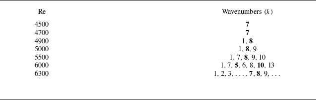
. During this transition, the equatorial instability also exhibits multiple wavenumbers. These wavenumbers are presented in table 2 for various Reynolds numbers. The table shows only the dominant wavenumbers in the equatorial instability and the bold numbers show the most dominant wavenumbers. As the reversal of the propagation direction of the travelling spiral wave instability is completed at
 $Re=5340$
(cf. § 4.2), we observe that the equatorial instability exhibits multiple wavenumbers with
 $k=8$
being the most dominant, as can be also seen in figure 20(b) for
 $Re=5340$
. Table 2 shows that, at larger Reynolds numbers, the equatorial instability supports a range of wavenumbers with multiple dominant modes. This multi-mode equatorial instability can be seen in figure 20(c) for
 $Re=6300$
, which is the largest Reynolds number analysed on the TWI branch in the present work. We can also observe a multi-mode rotating spiral instability at larger
 $Re$
, as shown in figures 20(b) and 20(c), which results in the chaotic state of the flow, discussed in the following section.
Dominant wavenumbers present in the equatorial instability for various Reynolds numbers on the TWI branch. The bold number represents the most dominant mode/s, and the dot-dot indicates many other modes.

Figure 21 shows the contours of the azimuthal vorticity along the
 $\theta$
direction, at the mid-radius and
 $\phi =0$
with time, for various Reynolds numbers on the EI branch. As mentioned previously (refer to § 4.3), the EI branch exhibits a two-vortex structure at the equator at
 $Re = 4500$
, resulting from the radial jet hitting the outer sphere at the equator. This results in twin jets above and below the equator (cf. § 4.3), as shown in figure 17. At
 $Re = 4500$
, the flow is steady and axisymmetric, as shown in figure 21(a). At
 $Re = 4750$
, the equatorial jet and the twin jets become unstable due to the oscillatory instability in the radial jet. This instability is clearly evident in figure 21(b). At the Reynolds number is increased to
 $Re = 5750$
, we also observe a weak rotating azimuthal instability appearing in the vicinity of the equator, which can be seen in figure 21(c). This structure is formed due to twin jets above and below the equator (cf. § 4.3), as shown in figure 17. This instability is different from the one observed on the TWI branch, as the flow exhibits a two-vortex structure for all the cases on the EI branch. Above
 $Re=4750$
, the two-vortex region is analogous to an unsteady double-gyre flow, as can be seen in figures 17(f), 17(g) and 17(h). No such structure is observed on the TWI branch. At larger Reynolds numbers (
 $Re=5750$
and
 $6250$
), we also observe a weak spiral instability in the flow away from the equator, as shown in figures 21(c) and 21(d). Further studies are required to check whether this spiral instability grows and results in a chaotic flow, something that is not observed for the range of Reynolds numbers investigated in the present work. In the next section, we briefly discuss the phase space dynamics on the three branches of the flow.
Time series data of azimuthal vorticity contours at
 $r=(R_i+R_o)/2$
;
 $\phi = 0$
is plotted along
 $\theta$
from 0 to
 $\pi$
for Reynolds numbers (a)
 $4500$
, (b)
 $4750$
, (c)
 $5750$
and (d)
 $6250$
on the EI branch.

6. Phase space dynamics
Phase space trajectories showing a limit-cycle behaviour for the periodic flow at
 $Re=6250$
on the axisymmetric branch, where time delay
 $\tau = 350$
.

We have used the numerical probe data of various cases to reconstruct the phase space of the flow as the
 $Re$
value of the flow is varied. The phase space for each case is reconstructed using Cao’s time delay method (Cao Reference Cao1997). More details of the method can be found in the literature (Kennel et al. Reference Kennel, Brown and Abarbanel1992; Cao Reference Cao1997). In the present work, we have plotted three-dimensional phase space diagrams from the velocity magnitude timeseries. As discussed in the previous section, a weakly periodic, axisymmetric solution emerges when the Reynolds number is increased to
 $Re=6250$
, on the axisymmetric branch. Figure 22 shows the phase space diagram corresponding to
 $Re=6250$
on the axisymmetric branch. One axis of the phase space diagram is the velocity magnitude
 $u(t)$
while the other two are
 $u(t+\tau )$
and
 $u(t+2\tau )$
, where
 $\tau$
is the delay time,
 $\tau =350$
. We see that the phase space shows a limit-cycle behaviour corresponding to the axisymmetric periodic solution. This is the largest Reynolds number studied on the axisymmetric branch, and we have not seen any other bifurcation on this branch.
On the TWI branch, we have observed an azimuthal spiral instability of
 $k=7$
at
 $Re=4500$
. The flow is periodic and non-axisymmetric due to this mode. The timeseries data from a numerical probe has shown the presence of a fundamental frequency and its first harmonic (cf. figure 11), indicating it is a period-doubling bifurcation. The phase space corresponding to the
 $Re=4500$
exhibits closed orbits, shown in figure 23(a). During the direction-reversing bifurcation that starts at
 $Re\approx 4700$
, the orbits in the phase space diagram shown in figure 23(b) are spread out as other harmonics of the fundamental mode also appear in the flow (cf. figure 12). After the completion of the direction-reversing bifurcation, the flow exhibits multiple spiral instability modes as it reaches a chaotic state. The diagram for
 $Re=6300$
, shown in figure 23(c) exhibits the orbits filling the entire phase space indicating the chaotic nature of the flow.
Phase space trajectories for (a)
 $Re=4500$
, (b)
 $Re=4700$
and (c)
 $Re=6300$
on the TWI branch.

Phase space trajectories for (a)
 $Re=5000$
, (b)
 $Re=5750$
and (c)
 $Re=6250$
on the EI branch.

The EI branch exhibits a steady and axisymmetric flow at
 $Re=4500$
. The first bifurcation, which is a symmetry-breaking bifurcation, occurs at
 $Re=4750$
, where the flow exhibits an equatorial instability of wavenumber
 $k=7$
. The timeseries of the velocity magnitude shows a fundamental frequency along with its first harmonic (cf. Figure 18), indicating a period-doubling bifurcation. Figure 24(a) shows the phase space diagram for
 $Re=5000$
, exhibiting period-2 orbits corresponding to this period-doubling bifurcation. Figures 24(b) and 24(c) show the phase space plots respectively for the Reynolds numbers
 $5750$
and
 $6250$
. The phase spaces still exhibit a period-2 nature. As discussed in the previous section (cf. § 4.3), the equatorial instability of
 $k=7$
persists up to the largest
 $Re=6250$
studied in the present work. The flow at these large
 $Re$
exhibits weak spiral instability in the polar region but does not show a chaotic nature, as evident from the phase space diagrams of the flow at large
 $Re$
.
7. Summary and conclusion
This work examines the spherical Couette flow for a narrow-gap ratio of
 $\beta =0.24$
for a range of Reynolds numbers. We find that the flow is sensitive to initial conditions, and various combinations of the initial conditions are used to obtain different branches of the bifurcation diagram. Such strategies have been used previously in the literature for medium-gap ratios of Spherical Couette flows (Wimmer Reference Wimmer1976). We identify three branches in the bifurcation diagram, plotted in the
 $\langle u_r \rangle _{\phi }-{\textit {Re}}$
plane, namely: the axisymmetric branch, the TWI branch and the EI branch. Backward marching in Re along the EI branch shows hysteresis in the flow.
As the name suggests, the flow on the axisymmetric branch remains axisymmetric and steady up to a large range of Reynolds numbers
 $ ({\textit {Re}}\lt 6250 )$
. The flow undergoes a Hopf bifurcation at
 $Re=6250$
, where an axisymmetric periodic solution emerges. The flow at this branch shows a dominant equatorial jet for all the Reynolds numbers analysed on this branch in the present work. At
 $Re=4500$
, a branch, called TWI, separates from this axisymmetric branch, where the flow supports travelling spiral waves and an equatorial wave.
The flow on the TWI branch is dominated by an azimuthal spiral instability of wavenumber
 $k=7$
, along with an equatorial instability of the same wavenumber. As the
 $Re$
value of the flow is increased, the direction of propagation of the travelling wave reverses. This flow transition starts at
 $Re\approx 4700$
and completes at
 $Re\approx 5340$
. During this transition, the equatorial wave first exbhibits a dominant wavenumber of
 $k=8$
and later, at larger Reynolds numbers, supports multiple wavenumbers. Further analysis is required to understand the relation between the instability of the travelling wave and the polar instability on the EI branch. At large Reynolds numbers, the flow also exhibits a chaotic behaviour, which results from the appearance of the multiple wavenumbers in both spiral and equatorial instabilities in the flow.
The EI branch, which gets separated from the axisymmetric branch at
 $Re\approx 4500$
, exhibits a two-vortex structure at the equator. This two-vortex structure is caused by two jet streams above and below the equator. As the Reynolds number is increased, the flow exhibits period doubling, the twin jet streams become unstable and the flow becomes non-axisymmetric. Similar to the TWI branch, we observe a weak azimuthal wave of wavenumber
 $k=7$
at the equator. Unlike the TWI branch, we do not observe a chaotic state for the range of Reynolds numbers investigated in the present work. The flow also exhibits hysteresis on the EI branch. Reducing
 $Re$
on this branch does not result in the flow jumping back immediately on the axisymmetric branch for
 $Re\lt 4500$
. Instead, the EI branch gets extended backward to a very low
 $Re=400$
before the flow jumps back to the axisymmetric branch. A similar analysis needs to be done for other gap ratios to generalise the inferences made here. Larger gaps will be more susceptible to instability, and we expect the transition to turbulence to happen early. It will be interesting to see the equatorial jet instability for these larger annular gaps. Since the initial conditions significantly influence the flow topology, a similar investigation is required with alternative initial conditions to broaden the understanding of bifurcation behaviour and the potential emergence of additional branches.
Acknowledgements.
All the computations reported in the paper were carried out at PARAM Ananta Supercomputer at IIT Gandhinagar under the National Supercomputing Mission coordinated by the Ministry of Electronics and Information Technology (MeitY) and Department of Science and Technology (DST), Government of India.
Declaration of interests.
The authors report no conflict of interest.