I. INTRODUCTION
Nickel-based superalloys have excellent mechanical properties and high resistance to creep and fatigue at elevated temperatures Reference Reed1 and are thus widely applied in rocket engines, steam turbines for aerospace, and other challenging environments. Reference Pollock and Tin2 Addition of Al leading to precipitate of secondary phase, γ′ (Ni3Al), from the matrix of γ-Ni phase, exhibits superior high-temperature strength. Reference Divinski, Frank, Södervall and Herzig3 Trace amount of Mo can improve creep and oxidation resistance, and then enhance structure stability of Ni3Al (γ′) phase. Reference Wei, Gong, Huang and Zhou4 The Ni–Al–Mo system has since received intensive interest among academic and industrial circus. Reference Henry5–Reference Wakashima, Higuchi, Suzuki and Umekawa7 It is well known that both creep and oxidation resistance of any material are dependent on its diffusion behavior. Meanwhile, accurate composition- and temperature-dependent interdiffusion coefficients are prerequisite for predicting creep resistance as well as for quantitative description of microstructure evolution during various processes by using, i.e., phase-field simulation. Reference Wang, Sheng, Liu and Chen8,Reference Wang9 To our knowledge, there is limited experimental information about interdiffusivities for face centered cubic (fcc) Ni–Al–Mo alloys in the open literature. It is then necessary to conduct experimental measurements of interdiffusion coefficients in the fcc Ni–Al–Mo system.
Incorporating the single-phase diffusion couple technique Reference Dayananda and Kim10–Reference Sohn and Dayananda12 and Matano–Kirkaldy method Reference Kirkaldy13–Reference Kirkaldy, Weichert and Haq15 is one of the most widely used ways to obtain interdiffusivities for a ternary system. However, one major obstacle of the Matano–Kirkaldy method is its relatively low efficiency. Using the Matano–Kirkaldy method, only four independent interdiffusivities at the intersection point of every two diffusion paths can be determined. To obtain composition- and temperature-dependent interdiffusivities for a chosen ternary system, one has to design and prepare a large number of diffusion couples (this is very time-consuming and costly). Thus, this method is considered less efficient to meet the requirement of MGI (Materials Genome Initiative). Reference Kaufman and Ågren16,Reference Olson and Kuehmann17 To remedy this situation, a pragmatic numerical inverse method has recently been developed by Chen et al. Reference Chen, Zhang, Du, Tang and Huang18 in our group, which can be used to effectively create and evaluate interdiffusivities in ternary systems by using a single diffusion couple. Very recently, this numerical inverse method has been substantially improved and augmented to be applicable for many alloys ranging from binary to multicomponent systems. Reference Chen, Zhong and Zhang19 Consequently, this newly developed numerical inverse method in combination with single-phase diffusion couple technique can be utilized for high-throughput measurements of interdiffusivities in the Ni–Al–Mo ternary system. The major objectives of the present work are then (i) to perform high-throughput measurements and obtain interdiffusivities in an Ni-riched fcc Ni–Al–Mo alloy at 1273, 1373, and 1473 K by using the numerical inverse method together with 15 groups of single-phased Ni–Al–Mo ternary diffusion couples, (ii) to validate the resulting composition-dependent interdiffusivities by comparing with those obtained from the traditional Matano–Kirkaldy method, as well as simulated interdiffusion fluxes and composition profiles with experimental data, (iii) to plot three-dimensional (3-D) diffusivity planes for main interdiffusivities at different temperatures and derive activation energy planes accordingly.
II. EXPERIMENTAL PROCEDURE
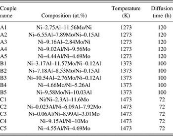
Nominal compositions of 15 Ni–Al–Mo diffusion couples of different compositions are listed in Table I. These compositions were carefully chosen based on calculated isothermal sections of the ternary Ni–Al–Mo system Reference Lu, Cui and Jin20,Reference Zhou, Wang, Chen, Liu and Napolitano21 to make sure that they are all falling into the fcc single-phase region. Pure aluminum (purity: 99.99 wt%), molybdenum (purity: 99.99 wt%), and nickel (purity: 99.99 wt%) were used as starting materials. Button samples of Ni–Al, Ni–Mo, and Ni–Al–Mo were prepared by arc melting pure elements under argon atmosphere with a nonconsumable W electrode (WKDHL-1, Opto-electronics Co. Ltd., Beijing, China). Samples were re-melted for five times to improve their homogeneities, and weight loss of each sample is negligible. After that, these buttons were linearly cut into blocks of 5 × 5 × 10 mm3 and sealed in quartz tubes under vacuum (4 × 10⁻⁴ bar). All blocks were homogenized at 1473 K for 10 days in an L4514-type diffusion furnace (Qingdao Instrument & Equipment Co. Ltd., China), followed by water quenching. Polished and cleaned blocks were bound together with molybdenum clamps to form 15 diffusion couples according to assembly listed in Table I. These couples were then sealed into quartz tubes under vacuum and annealed at 1273, 1373, and 1473 K for 120 h, 100 h and 72 h, respectively, in the L4514-type diffusion furnace prior to be quenched into cold water. Sections along the diffusion direction of annealed couples were polished and composition profiles along polished surfaces were measured by means of electron probe microanalysis (EPMA; JXA-8530, JEOL, Japan).
List of the nominal alloy compositions as well as annealing conditions for the fcc Ni–Al–Mo diffusion couples prepared in the present work.

III. METHODS FOR INTERDIFFUSIVITY EVALUATION
A. Numerical inverse method
Assuming in a hypothetical 1–2–3 ternary system (with 1 and 2 to be solutes while 3 be solvent; for the present work, 1 and 2 represents Al and Mo, and 3 for Ni), concentration evolution for component i (i = 1 or 2) is governed by Fick’s second law,
 $${{\partial {c_i}} \over {\partial t}} = {\partial \over {\partial x}}\left( {\tilde D_{i1}^3{{\partial {c_1}} \over {\partial x}} + \tilde D_{i2}^3{{\partial {c_2}} \over {\partial x}}} \right)\quad ,$$
where c
i
is the concentration of component i (i = 1 or 2), x is the diffusion distance, and t is the diffusion time.
 $\tilde D_{11}^3$
and
 $\tilde D_{22}^3$
are main interdiffusivities, while
 $\tilde D_{12}^3$
and
 $\tilde D_{21}^3$
are cross ones. According to Manning’s random alloy model,
Reference Manning22
the relationship between interdiffusivities
 $\tilde D_{ij}^3$
(i, j = 1 or 2) and mobility M
i
can be expressed as
 $$\eqalign{ & \tilde D_{ij}^3 = RT\left[ {{M_i}\varphi _{ij}^3 - {c_i}\left( {{M_1}\varphi _{1j}^3 + {M_2}\varphi _{2j}^3 + {M_3}\varphi _{3j}^3} \right)} \right] \cr & \quad\quad\quad\quad\quad \;\; + s\left[ {\left( {{M_i} - {c_1}{M_1} - {c_2}{M_2} - {c_3}{M_3}} \right){{2{c_i}RT\sum\nolimits_m {{M_m}\varphi _{mj}^3} } \over {{A_0}\sum\nolimits_m {{C_m}{M_m}} }}} \right]\quad , \cr}$$
where R is the gas constant and T is the temperature.
 $\varphi _{ij}^3$
is a thermodynamic factor which can be expressed by following equation:
 $$\varphi _{ij}^3 = {{{c_i}} \over {RT}}\left( {{{\partial {\mu _i}} \over {\partial {c_j}}} - {{\partial {\mu _i}} \over {\partial {c_3}}}} \right)\quad ,$$
where μ i is the chemical potential of component i which can be obtained from corresponding thermodynamic descriptions. According to our recent work, Reference Chen, Zhong and Zhang19 for a simple phase, whether accurate thermodynamic description is used or not has negligible effects on finally obtained interdiffusivities. The second term on the right side of Eq. (2) includes vacancy fluxes resulting from vacancy-wind effect. When s equals to 1, the effect of vacancy-wind is considered; while s equals to 0, this effect can be excluded. The parameter A 0 is a structure dependent factor. In present work, A 0 is selected to be 7.15 for crystals of a fcc structure. Reference Manning22
Generally, atomic mobility M i depends on concentration and temperature. In present work, expression of M i developed by Andersson and Ågren, Reference Kaufman and Ågren16 which is incorporated in DICTRA software, Reference Borgenstam, Engström, Höglund and Ågren23 was used,
 $${M_i} = {1 \over {RT}}\exp \left( {{{\Delta {G_i}} \over {RT}}} \right)\quad ,$$
where ΔG i can be expanded by Redlich–Kister polynomial
 $$\Delta {G_i} = {c_1}\Delta G_i^1 + {c_2}\Delta G_i^2 + {c_3}\Delta G_i^3 + {c_1}{c_2}\Delta G_i^{1,2} + {c_1}{c_3}\Delta G_i^{1,3} + {c_2}{c_3}\Delta G_i^{2,3} + {c_1}{c_2}{c_3}\Delta G_i^{1,2,3}\quad .$$
In DICTRA notation,
 $\Delta G_i^j$
is the end-member for diffusion of element i in element j (j = 1, 2, and 3), while
 $\Delta G_i^{1,2}$
,
 $\Delta G_i^{1,3}$
,
 $\Delta G_i^{2,3}$
, and
 $\Delta G_i^{1,2,3}$
are interaction parameters of element i in 1–2, 1–3, 2–3 binary and 1–2–3 ternary systems, respectively. The value of
 $\Delta G_i^j$
in Eq. (5) can be obtained from either experimental data, first-principles calculations, molecular dynamic simulation and/or some semiempirical methods. As for binary and ternary systems, these interaction parameters are treated as adjustable, which can be evaluated on the basis of composition profiles. Once estimation of adjustable parameter became available, interdiffusivity matrices can be calculated by integrating Eqs. (2)–(5), from which the Fick’s laws can be applied to make predictions of composition and interdiffusion flux profiles for experimental diffusion couples. Such predictions can be used to evaluate errors between predicted and experimental profiles,
Reference Chen, Zhong and Zhang19
 $$\min \left\langle {{\rm{error}}} \right\rangle = \min \left\langle {{w_{\rm{c}}} \cdot \sum\limits_{i = 1}^3 {\sum\limits_{j = 1}^{{\rm{Num}}} {{{\left( {|c_{ij}^{{\rm{cal}}} - c_{ij}^{\exp }|} \right)} \over {c_{ij}^{\exp }}}} } <$$><$$>+ {w_{\rm{J}}} \cdot \sum\limits_{i = 1}^3 {\sum\limits_{j = 1}^{{\rm{Num}}} {{{\left( {|\tilde J_{ij}^{{\rm{cal}}} - \tilde J_{ij}^{\exp }|} \right)} \over {\tilde J_{ij}^{\exp }}}} } } \right\rangle \quad ,$$
where Num is the number of experimental data.
 $c_{ij}^{{\rm{cal}}}$
,
 $\tilde J_{ij}^{{\rm{cal}}}$
,
 $c_{ij}^{\exp }$
, and
 $\tilde J_{ij}^{{\rm{exp}}}$
are the calculated and experimental compositions and interdiffusion fluxes of component i at the jth point, respectively. Interdiffusion fluxes for component i in a ternary system can be calculated on the basis of Fick’s first law,
Reference Dayananda24
 $$\tilde J_i^{{\rm{cal}}} = - \sum\limits_k^2 {\tilde D_{ik}^3} {{\partial {c_j}} \over {\partial x}}\left( {i = 1,2} \right)\quad ,$$
while experimental interdiffusion fluxes at any section
 $x'$
can be obtained from experimental concentration profiles by introducing normalized composition variable
 ${Y_i}$
,
 $\left( {{Y_i} = ({c_i} - {c^{\rm{L}}})/({c^{\rm{R}}} - {c^{\rm{L}}})} \right)$
,
Reference Whittle and Green25
 $$\tilde J_i^{{\rm{exp}}} = {{c_i^{\rm{L}} - c_i^{\rm{R}}} \over {2t}}<$$><$$>×\left[ {{{Y\prime_i} \cdot \int_{ - \infty }^{x\prime} {(1 - {Y_i})\,{\rm{d}}x + (1 - {{Y\prime_i})} \cdot \int_{x\prime}^\infty {{Y_i}\,{\rm{d}}x} } \right]\quad ,$$
where c L and c R are compositions at far left and right ends of diffusion couples, respectively. In general, weights of composition and interdiffusion flux in the minimization, w c and w J, are set to be 0.5. Appropriate algorithms (for instance, genetic algorithm) are used to iteratively change adjustable parameters to minimize errors defined in Eq. (6). When a least error between measured and calculated composition and interdiffusion flux profiles is achieved, interdiffusion coefficients can be finally determined according to Eqs. (2)–(5).
B. Matano–Kirkaldy method
The Boltzmann–Matano method was successfully extended to ternary and even to higher-order systems by Kirkaldy. Reference Kirkaldy13–Reference Kirkaldy, Weichert and Haq15 When one uses such method to determine 4 interdiffusivities in a ternary system, a pair of diffusion couples of which diffusion paths intersect at least at one common composition must be designed. Alternatively, with the assumption of constant molar volume over the diffusion zone, interdiffusion fluxes of each component can be obtained directly from composition profiles without using interdiffusivities. Based on the proposed relationship, Reference Dayananda24 interdiffusion fluxes of component i can be expressed as follows:
 $${\tilde J_i} = {1 \over {2t}}\int_{c_i^{ - \infty }{\rm{orc}}_i^{ + \infty }}^{{c_i}} {(x - {x_{\rm{M}}})\,{\rm{d}}{c_i}} \,(i = 1,2)\quad ,$$
where
 $c_i^{ - \infty }$
or
 $c_i^{ + \infty }$
is the terminal concentration for solute i at left and right sides of the diffusion couple, t is the diffusion time, and x
M is the distance of Matano plane,
Reference Kirkaldy13–Reference Kirkaldy, Weichert and Haq15
which can be determined from the following relation:
 $$\int_{c_i^{ - \infty }}^{c_i^{ + \infty }} {\left( {x - {x_{\rm{M}}}} \right)\,{\rm{d}}c = 0} \quad .$$
Based on Fick’s first law, interdiffusion flux
 ${\tilde J_i}$
can be also expressed by using interdiffusivities as Eq. (7). Combining Eqs. (7) and (9), the following relationship can be obtained:
 $${1 \over {2t}}\int_{c_i^{ - \infty }}^{c_i^{}} {\left( {x - {x_{\rm{M}}}} \right)\,{\rm{d}}{c_i}} = - \tilde D_{i1}^3\left( {{{\partial {c_1}} \over {\partial x}}} \right) - \tilde D_{i2}^3\left( {{{\partial {c_2}} \over {\partial x}}} \right)(i = 1,2)\quad .$$
Theoretically, positions of Matano planes of solutes 1 and 2 should be the same. However, Matano planes of different elements always deviate from each other to a certain extent, when determined by Eq. (10) according to experimental composition profiles. To solve this problem, Whittle and Green
Reference Whittle and Green25
introduced a normalized concentration parameter Y
i
 $\left( {{Y_i} = ({c_i} - {c^{\rm{L}}})/({c^{\rm{R}}} - {c^{\rm{L}}})} \right)$
. Thus Eq. (11) can be rewritten as follows:
 $$\eqalign{ & \tilde D_{11}^3 + \tilde D_{12}^3{{{\rm{d}}{c_2}} \over {{\rm{d}}{c_1}}} = {1 \over {2t}}{{{\rm{d}}x} \over {{\rm{d}}{Y_1}}}\left[ {\left( {1 - {Y_1}} \right)\int_{ - \infty }^x {{Y_1} \cdot {\rm{d}}x} + {Y_1}\int_x^{ + \infty } {\left( {1 - {Y_1}} \right) \cdot {\rm{d}}x} } \right]\quad , \cr & \tilde D_{22}^3 + \tilde D_{21}^3{{{\rm{d}}{c_1}} \over {{\rm{d}}{c_2}}} = {1 \over {2t}}{{{\rm{d}}x} \over {{\rm{d}}{Y_2}}}\left[ {\left( {1 - {Y_2}} \right)\int_{ - \infty }^x {{Y_2} \cdot {\rm{d}}x} + {Y_2}\int_x^{ + \infty } {\left( {1 - {Y_2}} \right) \cdot {\rm{d}}x} } \right]\quad . \cr}$$
Solving above equations, four ternary interdiffusivities,
 $\tilde D_{11}^3$
,
 $\tilde D_{12}^3$
,
 $\tilde D_{21}^3$
, and
 $\tilde D_{22}^3$
can then be obtained at intersection points of every two diffusion paths.
C. Evaluation of errors
For such numerical inverse method, one of the major concerns is uncertainty of determined interdiffusivities. Reference Xu, Chen, Zhang, Du and Tang26,Reference Chen, Xiao, Zhang and Du27 If there is no information about analytical solution, uncertainty evaluated via formula of error propagation is then appropriated. Taking the entire computation progress of adjustable parameters as a function f, uncertainties of such parameters can be evaluated according to the formula of error propagation Reference Léchelle, Noyan, Aufore, Arredondo and Audubert28
 $$u(f(A,B \ldots )) = \sqrt {\sum\limits_{\alpha = A,B \ldots } {{{(u(\alpha ))}^2}{{\left( {{{\partial f} \over {\partial \alpha }}} \right)}^2}} } \quad ,$$
where A and B… are relative factors in computation progress. Such relative factors, i.e., terminal compositions and positions of Matano planes, are usually determined from initial settings of diffusion couples or final observation of composition profiles of diffusion couples and uncertainties of u(A) and u(B), originated from their own process of determination. By applying minor changes to these relative factors individually and repeating computation progress for each factor, partial differential terms in the error propagation formula can be evaluated in a manner of numerical difference. Once uncertainties of optimized interaction parameters are retrieved, uncertainties of interdiffusivities along diffusion paths can be further considered according to error propagation formula and relation between adjustable parameters and interdiffusivities. Uncertainties of interaction parameters first propagate into atomic mobilities according to Eqs. (4) and (5) and finally propagate into interdiffusivities (or interdiffusivity matrices) with Eqs. (2) and (3). An attempt to evaluate uncertainties of interdiffusivities following the demonstration given above is carried out in the present work and an average representation is to be presented.
IV. RESULTS AND DISCUSSION
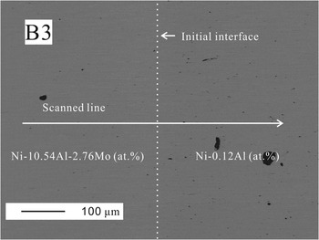
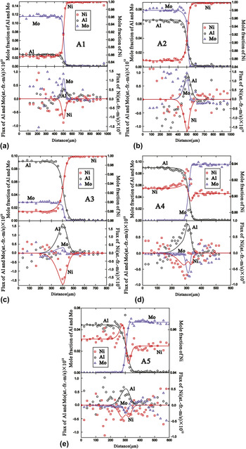
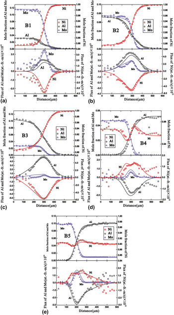
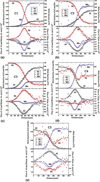
Taking consideration that all 15 diffusion couples prepared in the present work are designed to locate in the same fcc single-phase region, one typical microstructure of diffusion couples is given in Fig. 1. From Fig. 1, we noticed that the difference of contrast/brightness of image is negligible, i.e., the couple must locate in a one single-phase region. Figures 2–4 display measured composition profiles of Al, Mo, and Ni (denoted in symbols) for different diffusion couples annealed at 1273, 1373, and 1473 K, respectively. Variation in alloy composition is determined to be within ±1 at.% for each component. Besides, interdiffusion fluxes were obtained according to measured composition profiles based on Eq. (8), which are also denoted in symbols and shown in Figs. 2–4. Based on the numerical inverse method, composition-dependent interdiffusivities of fcc Ni–Al–Mo samples at 1273, 1373, and 1473 K were evaluated in the present work. During evaluation process, values for
 $\Delta G_{{\rm{Al}}}^{{\rm{Al}}}$
,
 $\Delta G_{{\rm{Al}}}^{{\rm{Ni}}}$
,
 $\Delta G_{{\rm{Ni}}}^{{\rm{Ni}}}$
, and
 $\Delta G_{{\rm{Ni}}}^{{\rm{Al}}}$
in Eq. (5) were taken directly from the work of Zhang et al.,
Reference Zhang, Du, Chen, Steinbach and Huang29
with
 $\Delta G_{{\rm{Mo}}}^{{\rm{Mo}}}$
,
 $\Delta G_{{\rm{Mo}}}^{{\rm{Ni}}}$
, and
 $\Delta G_{{\rm{Ni}}}^{{\rm{Mo}}}$
from Liu et al.
Reference Liu, Hu, Han, Lu and Wang30
Both
 $\Delta G_{{\rm{Mo}}}^{{\rm{Al}}}$
and
 $\Delta G_{{\rm{Al}}}^{{\rm{Mo}}}$
were assumed to be equal to
 $\Delta G_{{\rm{Al}}}^{{\rm{Al}}}$
and
 $\Delta G_{{\rm{Mo}}}^{{\rm{Mo}}}$
, respectively, for simplicity, due to lack of data. Binary (
 $\Delta G_{\rm{i}}^{{\rm{Al,Mo}}}$
,
 $\Delta G_{\rm{i}}^{{\rm{Al,Ni}}}$
,
 $\Delta G_{\rm{i}}^{{\rm{Ni,Mo}}}$
) and ternary (
 $\Delta G_{\rm{i}}^{{\rm{Al,Ni,Mo}}}$
) interaction parameters were considered as adjustable parameters and evaluated by measured composition profiles as described in Sec. III. A. All these parameters are listed in Table II. Meanwhile, Average relative errors of interdiffusivities,
 $\tilde D_{{\rm{AlAl}}}^{{\rm{Ni}}}$
,
 $\tilde D_{{\rm{AlMo}}}^{{\rm{Ni}}}$
,
 $\tilde D_{{\rm{MoAl}}}^{{\rm{Ni}}}$
, and
 $\tilde D_{{\rm{MoMo}}}^{{\rm{Ni}}}$
, obtained by the numerical inverse method were evaluated to be 2.4, 5.1, 16.1, and 1.7%, respectively.
Backscattered electron image of the microstructure of diffusion couple B3 annealed at 1373 K for 100 h.

Comparison between the experimental (denoted in symbols) and the model-predicted (denoted in lines) concentration profiles/interdiffusion fluxes of the diffusion couples annealed at 1273 K for 120 h in the present work: (a)–(e) represent diffusion couples A1–A5, respectively.

Comparison between the experimental (denoted in symbols) and the model-predicted (denoted in lines) concentration profiles/interdiffusion fluxes of the diffusion couples annealed at 1373 K for 100 h in the present work: (a)–(e) represent diffusion couples B1–B5, respectively.

Comparison between the experimental (denoted in symbols) and the model-predicted (denoted in lines) concentration profiles/interdiffusion fluxes of the diffusion couples annealed at 1473 K for 72 h in the present work: (a)–(e) represent diffusion couples C1–C5, respectively.

List of the evaluated kinetic parameters used in the numerical inverse method at 1273, 1373, and 1473 K.

By using obtained composition-dependent interdiffusivities, the composition profile of each diffusion couple at different temperatures can be predicted, as shown in Figs. 2–4 (denoted in solid lines). Moreover, interdiffusion fluxes along diffusion paths for all diffusion couples were also predicated and compared with experimental data presented in Figs. 2–4. As shown in these figures, our predicted concentration profiles are in good agreement with experimental data, while interdiffusion fluxes showed slight deviations from experimental data, especially those in Figs. 2 and 3. The major reasons for such deviations are as follows: (i) experimental interdiffusion fluxes were scattering widely and (ii) complex up-hill diffusion existed for Ni composition profiles.
To further check the reliability of resulting diffusivities, the Matano–Kirkaldy method was also utilized to obtain interdiffusivities at intersection points of every two diffusion couples. In the present work, there are 6 such intersection points at each temperature. Compositions for each intersection point are listed in Table III. As shown in Figs. 2–4, all these measured composition profiles of Al and Mo are nearly symmetric, whereas the standard Boltzmann function can be utilized to fit experimental profiles of these two elements. Smooth composition profiles c(x) relative to distance can then be produced according to
 $$c(x) = {{{A_1} - {A_2}} \over {1 + {{\rm{e}}^{{{x - {x_{\rm{M}}}} \over {dx}}}}}} + {A_2}\quad .$$
Diffusion coefficients in fcc Ni–Al–Mo alloys obtained by both the numerical inverse method and Matano–Kirkaldy method in the present work.

Here, A
1, A
2, and dx are fitting parameters for each composition profile. Moreover, positions of Matano plane x
M should be an average of those of Al and Mo in each diffusion couple. Fitted composition profiles of Ni were then obtained using relationship
 ${x_{{\rm{Ni}}}} = 1 - {x_{{\rm{Al}}}} - {x_{{\rm{Mo}}}}$
. Incorporating fitted Boltzmann functions and Matano–Kirkaldy method, four interdiffusivities at each intersection point were then obtained, as listed in Table III. Besides, relative errors for interdiffusivities determined using the Matano–Kirkaldy method have also been included in Table III.
To further validate these interdiffusivities, they are subjected to the following stable constraints of thermodynamics, Reference Onsager31 which express the stability of solid solution as follows:
 $$\tilde D_{{\rm{AlAl}}}^{{\rm{Ni}}} + \tilde D_{{\rm{MoMo}}}^{{\rm{Ni}}} > 0\quad ,$$
 $$\tilde D_{{\rm{AlAl}}}^{{\rm{Ni}}} \cdot \tilde D_{{\rm{MoMo}}}^{{\rm{Ni}}} - \tilde D_{{\rm{AlMo}}}^{{\rm{Ni}}} \cdot \tilde D_{{\rm{MoAl}}}^{{\rm{Ni}}} \,\,\ge\,\, 0\quad ,$$
 $${\left( {\tilde D_{{\rm{AlAl}}}^{{\rm{Ni}}} + \tilde D_{{\rm{MoMo}}}^{{\rm{Ni}}}} \right)^2} + 4 \cdot \tilde D_{{\rm{AlMo}}}^{{\rm{Ni}}} \cdot \tilde D_{{\rm{MoAl}}}^{{\rm{Ni}}} \,\,\ge\,\, 0\quad .$$
Inserting our data of interdiffusivities into Eqs. 15–17, we find that all of them fulfill these constraints, indicating that our present work is thermodynamically reliable.
Figures 5–7 show main interdiffusivities (
 $\tilde D_{{\rm{AlAl}}}^{{\rm{Ni}}}$
and
 $\tilde D_{{\rm{MoMo}}}^{{\rm{Ni}}}$
) and cross interdiffusivities (
 $\tilde D_{{\rm{AlMo}}}^{{\rm{Ni}}}$
and
 $\tilde D_{{\rm{MoAl}}}^{{\rm{Ni}}}$
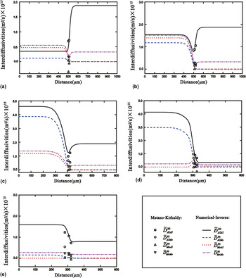
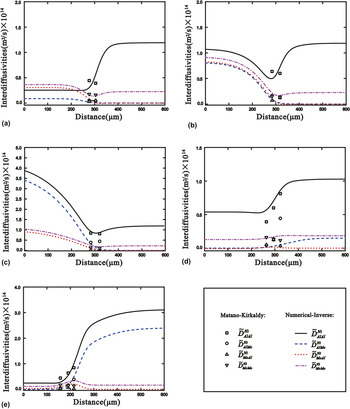
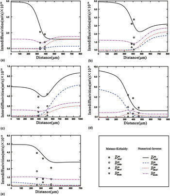
) of fcc Ni–Al–Mo samples obtained from the numerical inverse method (denoted in lines) as well as those from the Matano–Kirkaldy method (denoted in symbols) of each diffusion couple along entire diffusion paths at 1273, 1373, and 1473 K for comparison with detailed information listed in Table III. As can be seen from these figures and Table III, main interdiffusivities are positive in values at different compositions and temperatures. While for cross interdiffusivities, both positive and negative values may appear, indicating there is a chance to form a negative gradient of diffusion potentials versus composition.
Reference Liu, Zhang, Du, Xu and Jin32
Besides, the value of
 $\tilde D_{{\rm{AlAl}}}^{{\rm{Ni}}}$
is generally larger than that of
 $\tilde D_{{\rm{MoMo}}}^{{\rm{Ni}}}$
. This indicates that the diffusion rate of Al in the fcc Ni–Al–Mo samples is faster than that of Mo. Besides, main interdiffusivities obtained from the Matano–Kirkaldy method agree well with those from the numerical inverse method, while the agreement for cross interdiffusivities is less appreciable due to the fact that it is difficult to get accurate data.
Reference Xu, Chen, Zhang, Du and Tang26
Interdiffusivities along the entire diffusion paths for diffusion couples A1–A5 determined in the present work: (a) A1, (b) A2, (c) A3, (d) A4, and (e) A5. Here, lines are the results by using the numerical inverse method while symbols are the ones by using the Matano–Kirkaldy method.

Interdiffusivities along the entire diffusion paths for diffusion couples B1–B5 determined in the present work: (a) B1, (b) B2, (c) B3, (d) B4, and (e) B5. Here, lines are the results by using the numerical inverse method while symbols are the ones by using the Matano–Kirkaldy method.

Interdiffusivities along the entire diffusion paths for diffusion couples C1–C5 determined in the present work: (a) C1, (b) C2, (c) C3, (d) C4, and (e) C5. Here, lines are the results by using the numerical inverse method while symbols are the ones by using the Matano–Kirkaldy method.

Based on presently obtained composition-dependent interdiffusivities, 3-D diffusivity planes can be constructed. Figure 8(a) and 8(b) show surfaces of main interdiffusivities
 $\tilde D_{{\rm{AlAl}}}^{{\rm{Ni}}}$
and
 $\tilde D_{{\rm{MoMo}}}^{{\rm{Ni}}}$
over the selected composition range of fcc phase at 1273, 1373, and 1473 K. As shown in Fig. 8, two main interdiffusivities increased with temperature. The value of composition-dependent
 $\tilde D_{{\rm{AlAl}}}^{{\rm{Ni}}}$
increases with the concentration of Al. While the value of
 ${\tilde D}}_{{\rm{MoMo}}}^{{\rm{Ni}}}$
increases with concentrations of both Al and Mo. Besides, main interdiffusivities determined by the Matano–Kirkaldy method (symbols) are also plotted in Fig. 8 for comparison. It shows that main interdiffusivities at the same composition determined from both methods agree well with each other. Moreover, projection of the main interdiffusivities surface in Fig. 8 is exactly the diffusion path of each couple. Therefore, with such 3-D diffusivity surfaces, one can clearly know the evolution of interdiffusivities against composition and temperature, in addition to the diffusion path for each couple. It is generally believed that the higher the activation energy, the lower the diffusivity, and vice versa. The activation energy of fcc Ni–Al–Mo samples can be calculated according to the Arrhenius equation,
Reference Laidler33
 $$\tilde D_{ii}^{{\rm{Ni}}} = {D_0} \cdot {{\rm{e}}^{{{ - Q_{ii}^{{\rm{Ni}}}} \over {RT}}}}\quad ,$$
where D
0 is the diffusion constant and
 $Q_{ii}^{{\rm{Ni}}}$
is the activation energy. Based on constructed 3-D diffusivity planes of two main interdiffusivities at three temperatures, activation energies
 $Q_{{\rm{AlAl}}}^{{\rm{Ni}}}$
and
 $Q_{{\rm{MoMo}}}^{{\rm{Ni}}}$
for main interdiffusivities
 $\tilde D_{{\rm{AlAl}}}^{{\rm{Ni}}}$
and
 $\tilde D_{{\rm{MoMo}}}^{{\rm{Ni}}}$
can be evaluated. Figure 9 shows corresponding 3-D surfaces of activation energies. Moreover, contour lines are also superimposed in this figure. As shown in Fig. 9, the value of
 $Q_{{\rm{AlAl}}}^{{\rm{Ni}}}$
is inversely proportional to the composition of Al. Meanwhile, the value of
 $Q_{{\rm{MoMo}}}^{{\rm{Ni}}}$
decreases as both contents of Al and/or Mo. This tendency of variation is entirely contrary to that of main interdiffusivities.
Composition-dependent main interdiffusivities surfaces at 1273, 1373, and 1473 K in the 3-D space, compared with the results due to the Matano–Kirkaldy method: (a)
 ${\log _{10}}\tilde D_{{\rm{AlAl}}}^{{\rm{Ni}}}$
and (b)
 ${\log _{10}}\tilde D_{{\rm{MoMo}}}^{{\rm{Ni}}}$
.

Activation energy surfaces for the obtained composition-dependent interdiffusivities over the investigated composition range: (a)
 $Q_{{\rm{AlAl}}}^{{\rm{Ni}}}$
and (b)
 $Q_{{\rm{MoMo}}}^{{\rm{Ni}}}$
. The lines are the contour lines for activation energy.

V. CONCLUSIONS
Fifteen fcc Ni–Al–Mo ternary diffusion couples at 1273, 1373, and 1473 K were carefully prepared, from which the composition profile of each component was measured by EPMA technique. Based on the recently proposed numerical inverse method, composition-dependent interdiffusivities in fcc Ni–Al–Mo samples at 1273–1473 K over a selected composition range were determined. Obtained composition- and temperature-dependent interdiffusivities satisfy stable constraints of thermodynamics and agree well with results evaluated by the traditional Matano–Kirkaldy method. Moreover, our prediction of composition profiles and interdiffusion fluxes based on presently evaluated concentration-dependent interdiffusivities can reproduce measured data reasonably. These facts indicate that presently evaluated interdiffusivities in fcc Ni–Al–Mo samples are reliable. Furthermore, based on constructed main interdiffusivity planes at different temperatures, composition-dependent activation energies for main interdiffusivities were evaluated, from which activation energy planes over investigated composition ranges were also constructed.
ACKNOWLEDGMENTS
Financial support from National Natural Science Foundation for Youth of China (Grant No. 51301208), National Natural Science Foundation of China (Grant No. 51429101), and Hunan Provincial Natural Science Foundation for Youth of China (Grant No. 2015JJ3146) is greatly acknowledged. Lijun Zhang acknowledges project supported by State Key Laboratory of Powder Metallurgy Foundation, Central South University, Changsha, China.