




No CrossRef data available.
Early adolescent through young adult alcohol and marijuana use trajectories: Early predictors, young adult outcomes, and predictive utility
Published online by Cambridge University Press: 13 April 2004
Abstract
The present study takes a developmental approach to subgrouping and examines the trajectories of substance use from early adolescence through young adulthood among a community sample of 481 individuals. The patterns of use were examined, subgroups were identified separately for men and women and for alcohol and marijuana, and psychosocial predictors and psychopathology outcomes that differentiated the groups were identified. The results revealed three substantially overlapping subgroups for both alcohol and marijuana: early onset, late onset, and nonuser. Although the general patterns of which dependent variables were related to group were similar for alcohol and marijuana, a closer examination revealed important subgroup differences. For alcohol use, the early-onset group was more dysfunctional in terms of predictors and outcomes whereas the late-onset and nonuser groups were better adjusted. In contrast, for marijuana, the early- and late-onset groups were both more dysfunctional than the nonuser group. In a final analysis, we examined the predictive utility of our developmental approach to subgrouping compared to a traditional, static approach.This research was supported by NIH National Research Service Award DA07304 from NIDA, Grant DA05312-10 from NIDA, NIH General Clinical Research Center Grant M01 RR026202, and a University of Kentucky Research Challenge Trust Fund Fellowship awarded to Kate Flory.
Information
- Type
- Research Article
- Information
- Copyright
- © 2004 Cambridge University Press
The identification of subgroups within a disorder as a means to further our understanding of the disorder is traceable as far back as Kraepelin (1904). This classification approach has been used successfully in many areas including schizophrenia (e.g., Kraepelin, 1904; Roy, Merette, & Maziade, 2001), antisocial behavior (e.g., Moffitt, 1993), depression (e.g., Garland & Weiss, 1995), and substance abuse (e.g., Cloninger, 1987). It consists of identifying one or several characteristics (e.g., age of onset, response to treatment) that distinguish between groups of individuals with a common behavior or problem syndrome. The clinical and research implications for subgrouping are well established. Knowledge of subgroups can facilitate diagnosis and expedite treatment. This information may also provide a more accurate guide as to the expected course of a disorder or behavior. Moreover, the delineation of subgroups can help researchers better understand the etiology of psychological disorders and behaviors.
Many of the most commonly used classification schemes are based on static variables that are measured cross-sectionally. There are limitations to this approach, especially when studying disorders with child and adolescent onset. In our study, we take a prospective, developmental approach to substance use subgrouping in a large community sample. Using a developmental trajectory procedure (Nagin, 1999), we first identify subgroups based on patterns of alcohol and marijuana use from early adolescence through early adulthood. Then, we examine the validity of our subgroups by identifying predictors (e.g., school factors, conduct problems) and psychological outcomes (e.g., substance use disorders) associated with group membership. Finally, we examine whether our subgroups predict substance dependence above and beyond three static variables that are typically used to delineate subgroup membership (e.g., gender, age of onset, severity of lifetime use).
Current Approach to Subgrouping
Most subgrouping efforts have been based on one or more variables measured cross-sectionally and often retrospectively. Individuals have been classified based on age of onset, family history, symptom severity, psychiatric comorbidity, scores on screening inventories, personality characteristics, and many other variables. However, there may be important aspects of change over time that static variables do not capture. For example, two subgroups may have similar ages of onset; however, their patterns of the behavior over time may be very different. Along these lines, Chassin, Presson, Pitts, and Sherman (2000) distinguished between several subgroups of smokers, who were defined by their developmental patterns of smoking. It is important that the early-stable group and the experimenter group initiated smoking at approximately the same time (between 10 and 15 years of age). However, an examination of their smoking patterns revealed that the early-stable smokers remained heavy smokers into middle adulthood whereas the experimenters typically stopped smoking by age 20. A developmental approach to subgrouping, which takes into account change over time, may be able to more accurately group individuals with similar patterns of behaviors or symptoms.
Moffitt's (1993) theory of antisocial behavior demonstrates the advantages of the developmental approach to subgrouping. Moffitt describes two types of offenders: life-course persistent and adolescent limited. Life-course persistent antisocial behavior begins in childhood and continues through adolescence and into adulthood, and it is thought to result from neuropsychological problems interacting with a criminogenic environment. In contrast, adolescent-limited antisocial behavior, which begins in midadolescence and ends in early adulthood, is considered more normative. This form of antisocial behavior results from adolescents mimicking the behavior of those in the life-course persistent group. Moffitt presents evidence demonstrating that, over time, these two types of antisocial behavior have different correlates, trajectories, and outcomes. However, if the level of antisocial behavior during adolescence is the only variable that is measured, the two groups would appear quite similar.
Subgrouping Within Substance Use and Abuse Fields
The fields of alcohol and drug use and related problem behaviors (e.g., binge drinking) and disorders (e.g., alcoholism) have relied very heavily on subgrouping. Most of the subgrouping research in these areas has been conducted with adults and has focused on alcoholism. Perhaps the most widely known alcoholism subgrouping distinction was first proposed by Cloninger (1987) and later modified by Babor, Dolinsky, Meyer, Hesselbrock, Hofmann, and Tennen (1992). These researchers theorized that adult alcoholics can be classified into two distinct subgroups: Type I(A) and Type II(B). Type I(A) alcoholics have a later onset of alcoholism (>age 25), few first-degree relatives who are alcoholics, less severe dependence, few symptoms of co-occurring psychopathology, less psychosocial impairment, and more feelings of guilt about their alcohol use. Type I(A) alcoholics also tend to be low in impulsivity and novelty seeking and have few early risk factors (e.g., conduct disorder [CD]). In contrast, Type II(B) alcoholics have an earlier age of onset of alcoholism (<age 25), a stronger family history, more childhood conduct problems, more severe dependence, multiple drug abuse, and co-occurring psychiatric disorders, especially antisocial personality disorder. Type II(B) alcoholics are also typically male and high in impulsivity and novelty seeking (Babor, 1996; Ball, 1996). The Type I(A)/Type II(B) distinction has resulted in quicker diagnoses, successful treatment matching efforts (e.g., Litt, Babor, Del Boca, Kadden, & Cooney, 1992), and a clearer understanding of the mechanisms leading to alcoholism.
Although widely accepted, these substance use categorizations appear to have several limitations. The subgroup distinctions are primarily based on static, often retrospective, variables measured in adulthood (i.e., age of onset, family history, psychiatric comorbidity, personality), after substance use problems are already present. Most of these substance use subgrouping theories make no effort to examine or take into account patterns of use over time or the developmental progression from substance use to problem use/abuse. Thus, it may be that these theories are missing aspects of change over time that, if examined, would contribute to a more complete picture of substance use. The reliance on retrospective information to guide subgrouping efforts may also be problematic because it may be particularly difficult for established alcoholics or drug abusers to accurately recall childhood variables, such as age of substance initiation, on which the subgrouping schemes are often based.
Most importantly, however, in the substance use/abuse subtyping literature, adolescent substance use has generally received very little attention. This is an important oversight because epidemiological studies show that substance use begins very early. In fact, national survey data (e.g., Johnston, O'Malley, & Bachman, 1996a) suggest that drinking onset and first intoxication usually occur between Grades 7 and 10, and first marijuana experimentation typically occurs between Grades 9 and 11. Given this, it is likely that subgroup differences may actually be apparent beginning in early adolescence. Researchers who focus only on substance use and abuse after the age of 25 may thus be overlooking a wealth of information that may provide crucial answers about the onset, etiology, and course of lifetime substance use problems. The early identification of substance use subgroups also has implications for the prevention of later substance use problems, perhaps before a lifetime of negative consequences has accrued.
Only a few researchers have applied substance use/abuse subgrouping schemas to adolescents. Tarter, Kirisci, and Mezzich (1997) classified adolescent alcohol abusers into two subgroups based on 10 domains (e.g., severity of use, comorbid diagnoses) encompassed in the Drug Use Screening Inventory. Similarly, Weber, Graham, Hansen, Flay, and Johnson (1989) classified adolescents into two groups (Type I and Type II) based on 16 constructs related to alcohol use, including negative expectancies, access to alcohol, and number of friends who use. Babor, Webb, Burleson, and Kaminer (in press) examined six different ways (using gender, age of onset, family history, externalizing disorders, internalizing disorders, and temperament) for classifying adolescent marijuana abusers. As with adult substance use, however, these studies have relied primarily on static, cross-sectional variables to establish the subgroups. As discussed, there may be limitations to this static approach. In contrast, two recent studies have taken a more developmental approach to this issue.
Using a large community sample, Chassin et al. (2000) identified subgroups characterized by trajectories of smoking behavior from age 11 to 31. The authors empirically identified four groups (early stable smokers, late stable smokers, experimenters, and quitters) and demonstrated that the groups could be distinguished by a number of psychosocial variables measured in adolescence and young adulthood. In a study using the same methodology, Chassin, Pitts, and Prost (2002) examined the developmental trajectories of binge drinking from adolescence to emerging adulthood among children of alcoholics and controls. The authors identified four subgroups (early heavy, late moderate, infrequent, and nonbingers) and again demonstrated that the groups differed on a number of relevant psychosocial variables.
Finally, one study has examined the developmental trajectories of frequent binge drinking from late adolescence through young adulthood. Schulenberg, O'Malley, Bachman, Wadsworth, and Johnston (1996) used cluster analysis to place young adults into subgroups based on their drinking behavior between the ages of 18 and 24. Six groups emerged (never, rare, chronic, decreased, increased, and “fling”) that differed on a number of important variables, including problems with alcohol, attitudes about drinking, and illicit drug use.
The Present Study
The purposes of the present study are threefold. First, we address the limitations of prior attempts at substance use subgrouping among adults while replicating and extending Chassin and colleagues' work with adolescents. Using the same empirical developmental approach to subgrouping as Chassin et al. (2000, 2002; Nagin, 1999), we look at substance use over a 9-year period between ages 11 and 12 (6th grade) and ages 19–21. Our study differs from Chassin et al. (2000, 2002) in that we examine substance use, rather than bingeing, which focuses on only one specific aspect of substance use. In addition, we identify trajectories and subgroups separately for alcohol and marijuana and for men and women. Although our study differs from Chassin's work in these ways, we expect our trajectory findings to be consistent with hers in identifying at least three subgroups: a group that initiated substance use in early adolescence, a group that initiated use in late adolescence/early adulthood, and an abstainer group.
We examine the trajectories of alcohol and marijuana use separately. Along with cigarettes, alcohol and marijuana are the most widely used substances between early adolescence and young adulthood. Recent epidemiological data found that 22% of 8th graders and 50% of 12th graders reported drinking alcohol in the past 30 days, whereas 16% of 8th graders and 36% of 12th graders reported using marijuana within the past 12 months (Johnston, O'Malley, & Bachman, 2002). Both alcohol and marijuana are considered “gateway” drugs; however, several theories suggest that adolescents progress from cigarette and alcohol use to marijuana use (e.g., Kandel, 2002). Although generally grouped together in studies examining risk factors and outcomes, there is some evidence (e.g., White, Xie, Thompson, Loeber, & Stouthamer–Loeber, 2001) that the risk factors associated with marijuana use may differ from those associated with alcohol use. Thus, it is important to separately examine the developmental patterns, predictors, and outcomes of these two substances.
We also separately examine the trajectories of substance use for males and females. There are substantial gender differences in the prevalence rates of substance use and substance use disorders according to the Diagnostic and Statistical Manual of Mental Disorders, 4th edition (American Psychiatric Association, 1994). However, it is important to note that gender differences in overall rates of use do not necessitate differences in use patterns or the risk factors and outcomes associated with use. These issues must be empirically examined in order to determine whether gender specific theories are necessary.
In the second part of our study, we demonstrate the validity of our substance use subgroups by examining psychosocial variables that are expected to differentially predict the groups prior to the onset of substance use. The variables we include have been identified by prior research to be key risk factors for adolescent substance use. In a thorough review, Hawkins, Catalano, and Miller (1992) found that academic failure, noncommitment to school, poor family relations, high sensation seeking, positive expectancies, and CD were strongly related to substance use. Several studies (e.g., Brown, Parks, Zimmerman, & Phillips, 2001) have also found an inverse relationship between church involvement and alcohol use.
In validating our substance use subgroups, we also examine group differences on several young adult outcomes. A number of studies have found early substance use to be associated with deleterious outcomes, including later substance dependence, antisocial personality disorder, and arrests (e.g., Franken & Hendriks, 2000; McGue, Iacono, Legrand, Malone, & Elkins, 2001). Based on these findings and the research on risk factors, we hypothesize that the trajectory groups with the earliest onset of substance use will have the most negative risk factors and deleterious outcomes whereas the abstainer groups will be adjusted the best.
In the third part of the study, we compare the utility of the developmental approach to subgrouping with that of a retrospective static approach by examining whether our substance use subgroups predict substance dependence above and beyond several static variables used to establish subgroups. Up to this point, we and many others have assumed that a developmental approach would outperform the more standard, retrospective approach. This, however, is an empirically testable hypothesis.
Method
Participants
The 481 participants in the current study were part of a 10–12 year longitudinal examination of the etiological pathways to substance use, deviant behavior, and psychopathology. Participants were originally recruited for a study designed to test the effectiveness of Project DARE. However, the DARE intervention was found to have no effects on any program targets either 5 (Clayton, Cattarello, & Johnstone, 1996) or 10 (Lynam, Milich, Zimmerman, Logan, Martin, Leukefeld, & Clayton, 1999) years later, indicating that the community sample was appropriate for following prospectively.
Participants were first assessed via written questionnaires beginning in the 1987–1988 school year prior to starting the 6th grade (see Clayton et al., 1996, for a detailed description of the initial recruitment and assessment procedures). One hundred percent of schools and approximately 93% of all 6th graders in Lexington, Kentucky, participated in this original assessment. Follow-up data were collected from participants over a 5-year period after each school year from 6th through 10th grade (ages 11–12 through 15–16). Individuals in the current study completed questionnaires on at least three of these five occasions (post 6th grade, 7th or 8th grade, and 9th or 10th grade). Participants also completed a mailed survey at ages 19–21 (M = 20.1) and an extensive laboratory protocol at ages 20–22 (M = 21.0).
Due to resource limitations, we only assessed 481 individuals in the intensive laboratory phase of our study (ages 20–22). The 481 individuals who participated in the laboratory protocol were selected from the larger sample of 1,017 who had completed at least three of the school questionnaires and the mailed survey at ages 19–21. Individuals were randomly selected for the laboratory protocol with some oversampling of heavy users in order to compensate for previous sample attrition. Attrition analyses were conducted to examine the similarity of the laboratory sample of 481 to the 536 individuals who were also eligible for, but did not participate in, the laboratory protocol. We examined whether the 481 participants differed from the 536 on race, gender, or pre-6th grade past month, past year, and lifetime cigarette, alcohol, and marijuana use. The only significant differences were that individuals in the laboratory sample were more likely to be male, χ2 (1, N = 1,017) = 18.60, p < .001, and reported more pre-6th grade lifetime and past month use of alcohol than did the 536 individuals, F (1, 990) = 3.97, p < .05, and F (1, 1005) = 4.81, p < .05, respectively.
We also conducted attrition analyses to examine whether the 1,017 participants eligible for the laboratory protocol were comparable to the 642 participants who began the study prior to the 6th grade but who did not complete three of the five school questionnaires and thus were not eligible for continuation in the study. Individuals who did not complete three school questionnaires were more likely to be male, χ2 (1, N = 1,669) = 18.13, p < .001, and as expected, had significantly more past month, past year, and lifetime use of cigarettes, alcohol, and marijuana (F range = 4.81–47.93, all ps < .05). Although this pattern of selective attrition is typical of prospective studies with community samples, we attempted to compensate for the attrition by oversampling heavy users for the laboratory protocol. This was at least partially successful, because in a comparison of the 481 participants in the laboratory sample to the 642 who did not have three school questionnaires, the only significant differences were that the 642 reported more past year and lifetime use of cigarettes, F (1, 1,111) = 14.19, p < .001, and F (1, 1,105) = 27.40, p < .001, respectively, and greater lifetime use of marijuana, F (1, 1,110) = 6.98, p < .01.
The 481 young adults in the present study were from a metropolitan area of 330,000 people. Two hundred forty-one (50.1%) of the participants were men. The racial composition of the sample was 79.2% Caucasian, 15.8% African American, and 5% other. The majority of the participants (70%) had attended at least some college, and 21% had graduated from high school but not attended college. Only 9% of the sample reported not having graduated from high school. Over 73% of the sample was currently employed and 44% of those employed worked full-time (≥35 hr/week). Approximately 81% of the sample reported earning less than $900 per month, and 37% indicated that they had been at the same job for over 1 year.
In terms of lifetime use of alcohol, marijuana, and illicit drugs, the study sample at ages 19–21 was comparable to 1994 national prevalence estimates for young adults (ages 19–28) as reported in the Monitoring the Future Study (Johnston, O'Malley, & Bachman, 1996b). The Monitoring the Future Study estimated lifetime rates for alcohol, marijuana, and illicit drugs to be 91, 54, and 33%, respectively, while lifetime rates in our sample were 88, 61, and 38% for these three categories.
Procedure
Between the ages of 19 and 21, individuals who had completed at least three of the five school questionnaires were sent a survey to be filled out and returned by mail. The survey asked questions about the frequency of current drug use, among other things. From those who returned the survey, a smaller sample (described above) was contacted by telephone and asked to participate in a 3- to 4-hr laboratory study. Prior to the laboratory visit, participants who agreed to be in this phase of the study were mailed a consent form and a description of the purpose of the study.
The laboratory protocol was administered by trained research assistants. During the visit, participants completed a Life History Calendar (LHC; Caspi, Moffitt, Thornton, Freedman, Amell, Harrington, Smeijers, & Silva, 1996), segments of the Diagnostic Interview Schedule (Robins, Cottler, Bucholz, & Compton, 1997), and other measures of psychosocial functioning and psychopathology. Ninety-eight percent (N = 470) of participants had data available on all measures included in this study. Participants were reimbursed for their participation in all phases of the study.
Measures
Substance use
In each follow-up school questionnaire and in the mailed survey, participants were asked six questions regarding their use of alcohol and marijuana. Participants selected from seven choices of how often they had used each substance in their lifetime, in the past year, and in the past month. For these questions, 0 = the participant had not drunk alcohol or smoked marijuana during the time period, 1 = 1–2 drinks/times smoked marijuana, 2 = 3–5 drinks/times, 3 = 6–9, 4 = 10–19, 5 = 20–39, and 6 = 40+. To develop the trajectories for the current study, we used the past month reporting period for alcohol use and the past year reporting period for marijuana use. The six data points for the trajectories included post-6th grade (ages 11–12), post-7th (ages 12–13), post-8th (ages 13–14), post-9th (ages 14–15), post-10th (ages 15–16), and ages 19–21.
Predictor variables
With one exception, each of the predictor variables was taken from the school questionnaire administered to participants prior to 6th grade. CD symptoms prior to 6th grade were calculated from the retrospective LHC (Caspi et al., 1996) that participants completed during the laboratory interview (age 21).
School factors
This variable was a composite of a single item measuring school performance and a six-item scale measuring school commitment. The item and the scale were standardized and summed to form the composite. For performance, the item asked participants to assess how well they were doing in school overall. Response categories ranged from 1 (not at all well) to 4 (very well; M = 3.22, SD = 0.62). For commitment, the scale assessed how students felt about their school experience (e.g., “I do not look forward to school.”). Responses were measured on a 5-point continuum ranging from 1 (agree strongly) to 5 (disagree strongly) and items were coded such that higher scores on the scale reflected greater school commitment (M = 3.16, SD = 0.92). The coefficient alpha of this scale was .75. School performance and school commitment were moderately correlated (r = .26, p < .001). Higher scores on the composite variable represent better school performance and greater school commitment.
Church involvement
Participants were asked two questions regarding their frequency of attendance at church and the importance of this. For the frequency item, responses were measured on a 4-point continuum ranging from 1 (never) to 4 (once a week or more). For the importance item, responses were also measured on a 4-point continuum ranging from 1 (not important) to 4 (very important). To form a composite score for church involvement, the two items (r = .49) were averaged. Higher scores on this composite (M = 3.01, SD = 0.89) reflect greater church involvement.
Self-esteem
Participants' self-esteem was assessed with the 10-item Rosenberg Self-Esteem Scale (Rosenberg, 1965). Items included, “I feel that I am an important person” and “There are many good things about me.” Responses were measured on a 5-point continuum ranging from 1 (disagree strongly) to 5 (agree strongly) and coded such that higher scores indicated higher levels of self-esteem. As in previous studies, the scale (M = 3.97, SD = 0.59) was reliable with a coefficient alpha of .75.
Family relations
This 7-item scale measured how close the participants felt to their parents or guardians and the quality of these relationships (e.g., “Do you get a lot of attention at home?”). Responses were made on a 5-point continuum ranging from 1 (no, never) to 5 (yes, most of the time) with higher scores indicating better family relations. The coefficient alpha of this scale (M = 4.36, SD = 0.72) was .83.
Peer pressure resistance
This 7-item scale measured participants' ability to resist negative peer pressure (e.g., “If your best friend was skipping school, would you skip too?”). Responses were made on a 5-point continuum ranging from 1 (definitely would) to 5 (definitely not) with higher scores indicating a stronger ability to resist or ignore peer pressure. The coefficient alpha for this scale (M = 4.39, SD = 0.76) was .87.
Sensation seeking
Sensation seeking was measured using 18 items that were taken from Zuckerman's (1994) 40-item sensation seeking scale. Based on factor analyses, the four to six items most reflective of each of the four dimensions of Zuckerman's scale (i.e., Thrill and Adventure Seeking, Boredom Susceptibility, Experience Seeking, and Disinhibition) were included in our scale. To facilitate understanding among our young participants, these questions were adapted from the original forced choice format to one in which the participants indicated their level of agreement with a single statement (e.g., “I like to jump off high diving boards.”). Responses ranged from 1 (strong disagreement) to 5 (strong agreement), and all items were coded such that higher scores represented greater sensation seeking. The coefficient alpha of our scale (M = 2.87, SD = 0.59) was .74.
Expectancies for alcohol and marijuana use
These two composite variables were each composed of two scales that measured positive and negative expectancies separately. For negative expectancies, five-item scales assessed the extent to which participants expected the use of alcohol and marijuana to lead to negative outcomes (e.g., “Smoking marijuana makes a person lose their friends.” “Drinking alcohol makes a person do poorly in school.”). Responses were measured on a 5-point continuum ranging from 1 (strongly agree) to 5 (strongly disagree) with higher scores indicating fewer negative expectancies. The coefficient alphas of the negative expectancies scales for alcohol (M = 1.74, SD = 0.74) and marijuana (M = 1.55, SD = 0.67) were .78 and .76, respectively. For positive expectancies, eight-item scales assessed the extent to which participants expected the use of alcohol and marijuana to lead to positive outcomes (e.g., “How much does smoking marijuana help a person to have fun with friends?” “How much does drinking alcohol help a person to face a difficult situation?”). Responses were measured on a 4-point continuum ranging from 1 (does not help at all) to 4 (helps very much) with higher scores indicating more positive expectancies. The coefficient alphas of these scales were .88 for positive alcohol expectancies (M = 1.30, SD = 0.54) and .91 for positive marijuana expectancies (M = 1.29, SD = 0.60). The two alcohol expectancies scales were moderately correlated (r = .38, p < .001), as were the two marijuana expectancies scales (r = .39, p < .001). High scores on each expectancy variable reflected fewer negative expectancies and greater positive expectancies.
Variety of CD symptoms prior to 6th grade
This variable was calculated from participants' responses on a LHC completed during the laboratory interview. The LHC is a retrospective method for collecting data on a wide range of life events and behaviors (Caspi et al., 1996). In our LHC, we asked about the occurrence of delinquent acts (i.e., stealing, setting fires) beginning in 1986, when participants were in the 5th grade, up until the time of the laboratory protocol. Each year was broken into three 4-month segments and participants were asked about the occurrence and frequency of 15 different delinquent acts during these intervals. For the present study, we counted the total number of different delinquent acts that a participant reported as occurring prior to 6th grade (M = 0.83, SD = 1.17).
The LHC method capitalizes on advances in survey methodology and cognitive psychology to collect reliable time-linked retrospective data. The LHC uses visual aids, inquires about streams of events rather than isolated events, and contextualizes questions about life events by linking them to other events. Filling out the calendar requires no interpretation, inference, or judgment. During the periods sampled by our LHC, individuals were fully aware and active participants in the events. Each of these characteristics makes it likely that the data collected via the LHC will be an accurate and reliable assessment of the individuals' lives (Rutter, Maughan, Pickles, & Simonoff, 1998). As Brewin, Andrews, and Gotlib (1993) noted following their review of the literature on retrospective reports, “provided that individuals are questioned about the occurrence of specific events or facts that they were sufficiently old and well placed to know about, the central features of their accounts are likely to be reasonably accurate” (p. 94). In fact, previous studies (e.g., Caspi et al., 1996; Freedman, Thornton, Camburn, Alwin, & Young–DeMarco, 1988) and data from our project have documented the reliability and validity of the LHC.
Outcome measures
All of the outcome measures were drawn from data collected by interview and questionnaire during the laboratory protocol (ages 20–22).
Internalizing disorders, antisocial personality disorder, and substance use and dependence symptoms
Each of these variables was taken from the Diagnostic Interview Schedule (DIS-IV; Robins et al., 1997). The DIS is a structured interview developed for use by nonclinicians to assess the presence or absence of psychiatric disorders. The version of the DIS used in the current study corresponded with diagnoses included in the DSM-IV (American Psychiatric Association, 1994). Although the DIS has been changed periodically to correspond to the criteria of the most current version of the DSM, these changes do not alter the DIS as an assessment tool. Thus, the reliability and validity evidence is believed to be the same across versions. The DIS-II, which corresponded to the DSM-III, proved to have good sensitivity (.75), excellent specificity (.94), and moderate positive predictive power (.76; Robins, Helzer, Ratcliff, & Seyfried, 1982). A kappa analysis, which is a measure of agreement, was conducted to see how reliable the DIS was for administration by nonclinicians versus administration by psychiatrists. The kappa values ranged from a low of .4 (only for a diagnosis of panic disorder) to a high of 1 (for a diagnosis of anorexia nervosa) with all other diagnoses at least as high as .51 (Robins et al., 1982).
For the current study, participants were assessed for antisocial personality symptoms since age 15 and generalized anxiety, specific phobia, social phobia, depression, and alcohol and marijuana abuse and dependence symptoms within the last 12 months. We examined DSM-IV symptom counts for each of these areas rather than actual diagnosis because of the nonclinical status of our sample. For generalized anxiety, the symptom count for our participants ranged from 0 to 4 with a mean of 0.54, specific phobia ranged from 0 to 4 symptoms with a mean of 1.46, social phobia ranged from 0 to 4 symptoms with a mean of 1.22, and depression ranged from 0 to 9 symptoms with a mean of 1.41. For alcohol abuse, the symptom count ranged from 0 to 4 with a mean of 0.57, marijuana abuse ranged from 0 to 3 symptoms with a mean of 0.37, alcohol dependence ranged from 0 to 6 symptoms with a mean of 1.12, and marijuana dependence ranged from 0 to 6 symptoms with a range of 0.76. Finally, the symptom count for antisocial personality disorder ranged from 0 to 5 with a mean of 0.57.
For the present study, we combined the variables for generalized anxiety, specific phobia, social phobia, and depression (r = .17–.28, all ps < .001) to represent total internalizing disorder symptoms. We also combined alcohol abuse and dependence (r = .60, p < .001) and marijuana abuse and dependence (r = .72, p < .001).
Total arrests
Participants were asked by questionnaire how many times they had been arrested in their lifetime (M = 0.72, SD = 1.56).
Variables for comparison with static model of subgrouping
These variables were taken from the mailed survey (ages 19–21).
Severity of lifetime use
This variable was taken from the mailed survey and was measured separately for alcohol (M = 4.63, SD = 2.03) and marijuana use (M = 2.83, SD = 2.62). Participants were asked how often they had used the substance in their lifetime with responses ranging from 0 (none) to 6 (40 or more times).
Age of onset of substance use
The age of onset was measured separately for alcohol and marijuana use by one question that asked how old participants were when they first used the substance. For alcohol, age of onset ranged from 3 to 21 (M = 15.51, SD = 3.77) with 45 participants never having initiated by age 21. For marijuana use, age of onset ranged from 8 to 21 (M = 18.47, SD = 3.33) with 178 participants never having initiated use by age 21. In the analyses, two variables were needed to fully represent age of onset: a continuous variable for age of first use and a dichotomous variable for whether participants had ever used.
Statistical procedure
Nagin's (1999) method of modeling developmental trajectories was used to examine participants' longitudinal patterns of alcohol and marijuana use. This method is group based and assumes that the relevant population is composed of a mixture of distinct groups defined by their developmental trajectories. Nagin (1999) provides a detailed description of this statistical procedure. In short, longitudinal data are used to identify the number of groups that best fits the data and the shape of the trajectory for each group. It is then possible to calculate the probability of each individual in the sample being in each of the trajectory groups that make up the model. Individuals can then be assigned to the group to which their probability of belonging is the highest.
Results
We began by using Nagin's (1999) procedure to determine the number and shapes of the substance use trajectories, separately by gender and type of substance use (alcohol, marijuana), and to assign participants to the group to which they had the highest probability of belonging. Next, we conducted a series of 2 × 3 analyses of variance exploring gender and group differences on substance use and each of the predictor and outcome variables. For these analyses, we used a significance level of p < .01 to minimize the possibility of Type 1 errors. For each variable where the main effect of group was significant, we then examined all pairwise comparisons between the groups. For variables for which the Gender × Group interaction was significant, we conducted group pairwise comparisons separately for men and women to better understand the nature of the interaction. Finally, we examined whether our developmental subgroups predicted substance dependence above and beyond three static variables frequently used in subgrouping. All of the analyses were conducted separately for alcohol and marijuana.
Empirically identifying substance use trajectories
Substance use data from six time points (post-6th grade, ages 11–12; 7th grade, ages 12–13; 8th grade, ages 13–14; 9th grade, ages 14–15; 10th grade, ages 15–16; and ages 19–21) were used in each of the trajectory analyses, which were conducted separately for men and women and for alcohol and marijuana use. We used SAS PROC TRAJ (censored normal; Jones, Nagin, & Roeder, 2001) to model the trajectories as a function of the measurement wave, and we specified the highest order polynomial as quadratic. For each of the four trajectory analyses, we first specified two groups and then tested a series of models, increasing the number of groups and using the Bayes information criterion (BIC) to evaluate the model fit (Jones et al., 2001; Nagin, 1999). We rejected solutions that did not contain a nonuser group, because we had not specified this group a priori. With this stipulation, for all four analyses, a three-group solution was the most parsimonious and resulted in the maximum BIC. The resulting trajectories are displayed in Figures 1 and 2, with men and women presented on the same figure for each substance.

The alcohol use trajectories for men and women. For mean alcohol use, 0 = 0 glasses of alcohol in the past month, 1 = 1–2 glasses, 2 = 3–5 glasses, 3 = 6–9 glasses, and 4 = 10–19 glasses.

The marijuana use trajectories for men and women. For mean marijuana use, 0 = having smoked marijuana 0 times in the past year, 1 = 1–2 times, 2 = 3–5 times, 3 = 6–9 times, 4 = 10–19 times, 5 = 20–39 times, and 6 = 40+ times in the last year.
Alcohol
For men's and women's alcohol use (Figure 1), one group initiated alcohol use by 11–12 (early onset), another group initiated use by 15–16 (late onset), and a third group did not use alcohol at all over the course of the data collection (nonusers). For men, 40 participants fell into the early-onset alcohol group, 150 were assigned to the late-onset group, and 46 were placed in the nonuser group. For women, 59 were in the early-onset group, 133 fell into the late-onset group, and 42 were assigned to the nonuser group. There were no significant differences in group classification between men and women, χ2 (2, N = 470) = 4.84, p = .089. For men and woman assigned to the early-onset alcohol group, the average a posteriori probability of being in the group was .87 (SD = .16); for those in the late-onset group, the average probability was .88 (SD = .16); and for those in the nonuser group, the average probability was .68 (SD = .10).
From 11–12 through 14–15 years of age, the late-onset and nonuser groups were equivalent and had significantly less alcohol use than the early-onset group (Table 1). By 19–21, the two using groups (early onset and late onset) were equivalent in their levels of use and were significantly higher than the nonusers. These results were qualified by two significant Gender × Group interactions. At 13–14, early-onset men had significantly greater alcohol use than early-onset women, but the two other groups were equivalent across gender. At 15–16, early-onset and late-onset men had significantly more use than women in these groups, whereas men and women nonusers were equivalent.
Group and gender means and standard deviations and analyses of variance results for substance use by age

Marijuana
The trajectory groups for marijuana use (Figure 2) were similar to those for alcohol. For both men and women, one group initiated marijuana use before age 11–12 (early onset). A second group initiated marijuana use by age 14–15 (late onset), whereas a third group never used marijuana (nonusers). For men, 13 fell into the early-onset group, 132 were placed in the late-onset group, and 91 were assigned to the nonuser group. For women, 27 fell into the early-onset group, 99 were placed in the late-onset group, and 108 were assigned to the nonuser group. There was a significant difference in group classification between men and women for marijuana, χ2 (2, N = 470) = 11.06, p < .01, such that more women than men fell into the early-onset and nonusers groups and more men than women fell into the late-onset group. For men and women assigned to the early-onset marijuana group, the average a posteriori probability of being in the group was .89 (SD = .15); for those in the late-onset group, the average probability was .94 (SD = .11); and for those in the nonuser group, the average probability was .74 (SD = .07).
From age 11–12 through 13–14, the late-onset and nonuser groups were equivalent in marijuana use and had significantly less use than the early-onset group. At 14–15, 15–16, and 19–21, the three groups were all significantly different from one another in level of marijuana use (Table 1). By age 19–21, the late-onset group had the highest level of marijuana use. As with alcohol use, these results were qualified by two significant Gender × Group interactions (ages 12–13 and 13–14). At both time periods, early-onset men had a significantly higher rate of marijuana use than early-onset women whereas men and women's marijuana use between the other two groups was equivalent.
Group overlap
We examined the overlap between the marijuana and alcohol trajectory group assignments for men and women separately. For men, there was a strong association, χ2 (4, N = 236) = 78.82, p < .001. Sixty-one percent of cases fell along the diagonal. For the early-onset marijuana group, 10 of 13 cases were also in the early-onset alcohol group with the remaining three cases falling in the late-onset alcohol group. No participants in the early-onset marijuana group were in the nonuser alcohol group. The findings were similar for the early-onset alcohol group. Of the 40 participants in this group, 37 were in either the early-onset or late-onset marijuana groups. Upon collapsing the two onset groups within each type of drug, 73% of the cases fell on the diagonal. Of the off-diagonal cases, 86% (54 of 63) represented instances of early- or late-onset alcohol use in conjunction with membership in the nonuser marijuana group.
The results were similar for women. There was an association between the two sets of trajectories, χ2 (4, N = 234) = 69.37, p < .001. Fifty percent of cases fell along the diagonal. For the early-onset marijuana group, 22 of 27 cases were also in the early-onset alcohol group with 4 of the remaining 5 cases falling in the late-onset alcohol group. The findings were similar for the early-onset alcohol group. Of the 59 participants in this group, 50 of them were in either the early-onset or late-onset marijuana groups. Upon collapsing the two onset groups within each type of drug, 62% of the cases fell on the diagonal and of the off-diagonal cases, 88% (77 of 88) represented instances of early- or later onset alcohol use in conjunction with membership in the nonuser marijuana group.
Predicting the trajectory groups
For reference, bivariate correlations among and between the predictor and outcome measures are presented in Table 2.
Bivariate correlations among and between predictor and outcome measures

Alcohol
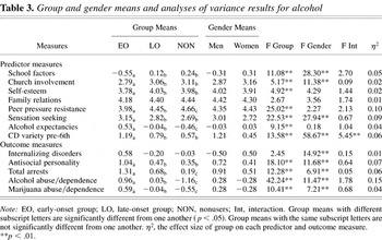
There were significant group differences on seven of the eight predictor variables, including school factors, church involvement, self-esteem, peer pressure resistance, sensation seeking, expectancies, and variety of CD symptoms prior to 6th grade (see Table 3). On five of the seven variables, the early-onset group differed from the late-onset and nonuser groups, which were not significantly different from each other. The early-onset group was significantly lower than the other two groups on school factors, church involvement, and self-esteem and higher than the other groups on sensation seeking and CD symptoms prior to 6th grade. On the remaining two variables, all three groups were significantly different from each other and the differences were linear: the early-onset group scored the lowest on peer pressure resistance and the highest on expectancies (high positive, low negative), the nonuser group scored the highest on peer pressure resistance and the lowest on expectancies, and the late-onset group scored between the other two. These results were qualified by a significant Gender × Group interaction for the variety of CD symptoms prior to 6th grade. Early-onset men had significantly more CD symptoms than men in the other two groups, which were equivalent in terms of CD symptoms. In contrast, there were no significant differences between the three women's groups in terms of CD symptoms.
Group and gender means and analyses of variance results for alcohol

Marijuana
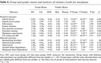
There were significant group differences on seven of the eight predictor measures, including school factors, self-esteem, family relations, peer pressure resistance, sensation seeking, expectancies, and variety of CD symptoms prior to 6th grade (Table 4). The majority of the differences occurred in a linear fashion, and all three groups were significantly different from each other on many of the variables. The early-onset group scored the lowest on school factors, self-esteem, family relations, and peer pressure resistance and the highest on expectancies; the nonusers scored the lowest on expectancies and the highest on school factors, self-esteem, family relations, and peer pressure resistance. The late-onset group scored between the other two groups on these variables. On the remaining two variables, the early- and late-onset groups were similar to each other but were significantly higher than the nonusers on both of the variables. There was one significant Gender × Group interaction: early-onset men demonstrated higher expectancies than early-onset women, whereas the other two groups were equivalent across gender.
Group and gender means and analyses of variance tesults for marijuana

Outcomes for the trajectory groups
Alcohol
There were group differences on four of the five variables, including antisocial personality symptoms, total arrests, and both alcohol and marijuana abuse/dependence (Table 3). All but one of these differences occurred in a linear fashion, with all three groups significantly different from each other on each of the variables. In these cases, the early-onset group demonstrated the most psychopathology and the most negative outcomes and the nonusers had the least. For antisocial personality disorder symptoms, the early-onset group was significantly higher that the other two groups, which were not significantly different from one another.
Marijuana
There were significant group differences for four of the five outcome measures of antisocial personality, total arrests, and alcohol and marijuana abuse/dependence (Table 4). On two of the four variables, the differences occurred in a linear fashion, with the early-onset group having the most arrests and alcohol abuse/dependence, the nonusers having the least, and the late-onset group between the other two groups. However, for the other two variables (antisocial personality and alcohol abuse/dependence), the early-onset and late-onset groups were not significantly different from each other but were different from the nonusers. The nonusers had fewer symptoms of antisocial personality disorder and less marijuana abuse/dependence.
Comparison with static model of subgrouping
The final analyses were conducted to examine whether our developmental model of subgrouping was able to predict substance dependence above and beyond three static variables (e.g., gender, age of onset, severity of lifetime use) that are frequently used to establish subgroups. These analyses were conducted separately for the alcohol and marijuana groups predicting the outcomes of alcohol and marijuana dependence, respectively. For both analyses, hierarchical multiple regression was used; the three static variables were entered in the first step, and the continuous probabilities of membership in the two substance using groups were entered in the second step. For alcohol dependence, the R2 value (.30) was significant (F = 46.64, p < .001) for the first step as was the change in R2 (.03) for the second step (F = 8.69, p < .001). For marijuana, the R2 value (.35) for the first step was significant (F = 58.87, p < .001), but the change in R2 (.00) for the second step (F = .81, ns) was not significant.1
For a more stringent comparison of the developmental approach with the traditional static method of subgrouping, we also ran the comparison analyses using dichotomized versions (at the mean) of the age of onset and lifetime severity of use, along with gender, entered in the first step, and the continuous probabilities of membership in the two substance using groups entered in the second step. This did not alter the results. For alcohol dependence, the R2 value (.34) was significant (F = 57.98, p < .001) for the first step as was the change in the R2 (.02) for the second step (F = 7.41, p < .01). For marijuana, the R2 value (.28) for the first step was significant (F = 43.59, p < .001), but the change in the R2 (.01) for the second step (F = 1.70, ns) was not significant. In addition, we ran the comparison analyses including a term, entered in the third step, representing the interaction of gender with the continuous probabilities of membership in the two substance using groups. There were no significant Group × Gender interactions.
Finally, we ran the comparison analyses entering the continuous probabilities of membership in the two substance using groups in the first step and the three static variables in the second step. Even reversing the order of entry, the static variables continued to contribute predictive utility above and beyond the probabilities of group membership. For alcohol dependence, the R2 value (.18) was significant (F = 49.66, p < .001) for the first step as was the change in the R2 (.14) for the second step (F = 22.91, p < .001). Similarly, for marijuana dependence, the R2 value (.19) for the first step was significant (F = 52.81, p < .001) as was the change in the R2 (.16) for the second step (F = 26.72, p < .001).
Discussion
Static variables, such as symptom severity, have long been successfully used to establish subgroups for substance use and other forms of psychopathology. Recently, however, there has been a strong push within the subgrouping literature to use a developmental approach, rather than the traditional static one, to classify individuals into groups. There are several disadvantages of the static approach. An examination of several developmental models for subgrouping (e.g., Chassin et al., 2000, 2002; Moffitt, 1993; Schulenberg et al., 1996) suggests that taking a static approach may overlook important aspects of change over time that could result in different groupings, if taken into account. In addition, the formation of subgroups based on variables measured at only one time point cannot account for the progression from a behavior to a problem or syndrome, which may have important implications for understanding the etiology and for developing appropriate interventions and treatments. Moreover, subgrouping based on retrospective variables may suffer from inaccurate reporting.
Given these disadvantages of traditional subgrouping efforts, we also used a developmental approach to identify subgroups based on individuals' substance use patterns from early adolescence through young adulthood. A number of our findings were quite informative. One unique aspect of our study was that we examined subgroups separately for alcohol and marijuana use. The number and shape of the trajectories of the alcohol and marijuana subgroups were similar. Group overlap was very high (e.g., early-onset marijuana users tended to be early-onset alcohol users), and the general patterns of predictor and outcome variables significantly related to group status were similar for alcohol and marijuana. As expected and consistent with prior research (e.g., Brown et al., 2001; Hawkins et al., 1992), the early factors of school and church involvement, self-esteem, peer pressure resistance, sensation seeking, expectancies, and conduct problems all significantly differentiated the alcohol and marijuana subgroups. The groups were also distinguished by differences in young adult outcomes, including alcohol and marijuana dependence, antisocial personality disorder symptoms, and number of arrests. This suggests that there is little specificity in the differential predictors of and outcomes associated with alcohol versus marijuana use. These findings are consistent with Jessor and colleagues' (Donovan & Jessor, 1985; Donovan, Jessor, & Costa, 1988; Jessor & Jessor, 1977) problem behavior theory, which states that there is a single common factor or syndrome that accounts for a number of adolescent problem behaviors, including alcohol and marijuana use and delinquent-type behavior. Further, these findings may suggest that, when put to the empirical test, theories that specify different predictors and outcomes for different types of substances may not stand up.
Likewise, it does not appear that different theories explaining men and women's substance use are necessary. Although we found that the overall levels of both alcohol and marijuana use were higher for men than women, the use patterns, subgroups, and predictor and outcome variables generally did not differ by gender.
Notably, however, there were several interesting trends in the specific patterns of the alcohol and marijuana group differences on the predictor and outcome measures. In the majority of the group comparisons for alcohol, the late-onset and nonuser groups were similar to one another, but both were significantly better adjusted than the early-onset group. A different pattern emerged for the marijuana subgroups. For most of the comparisons, the early-onset and late-onset groups were indistinguishable and were significantly more dysfunctional than the nonuser group. Thus, it appears that, for alcohol use, individuals who fare the worse are those who begin using alcohol at an early age and those who initiate use at a later age or who abstain altogether are at a relative advantage, both in terms of risk factors and adult psychosocial outcomes. In contrast, marijuana use initiated at any age between 6th grade (age 11–12) and age 20 is associated with a relative psychosocial disadvantage and a number of deleterious outcomes. These differences may relate to the contexts in which the two substances are typically used or differences in the availability and licitness of the substances. Alcohol is often widely available at social gatherings and is generally easily obtainable whereas an individual may have to go out of his or her way to obtain marijuana, which is illegal, less widely available, and often used surreptitiously.
Overall, our results are consistent with several prominent theories of subgrouping (i.e., Babor et al., 1992; Cloninger, 1987; Moffitt, 1993), suggesting that some aspects of these theories may be applicable to the understanding of adolescent through young adult substance use. In her theory of antisocial behavior, Moffitt (1993) recognizes two subgroups of offenders. Life-course persistent offenders are characterized by neuropsychological deficits, “difficult” temperament, poor family relations, problems with socialization, and negative outcomes. In contrast, adolescent-limited offenders are thought to be relatively well adjusted, perhaps even more than those who abstain altogether from antisocial behavior, although this last hypothesis remains controversial. Our early-onset groups correspond in many ways to Moffitt's (1993) life-course persistent group, as individuals were generally characterized by a number of family, social, and academic difficulties and several negative adult outcomes. Our alcohol late-onset group appears similar to Moffitt's (1993) adolescent-limited group because these individuals were better adjusted in terms of early risk factors and adult outcomes. However, our late-onset marijuana group was more dysfunctional. Unlike Moffitt's theory, we found that the nonuser group was, in many cases, adjusted the best. This finding may relate to our examination of trajectories of substance use, whereas Moffitt's theory deals with antisocial behavior. In fact, a recent study by Milich et al. (2000), using our data set, found that individuals who abstained from alcohol or marijuana use were not more psychologically impaired than experimenters and occasionally were better adjusted. Although our results are not entirely consistent with Moffitt's theory, many aspects of her theory could be usefully applied to substance use, particularly because antisocial behavior is highly associated with substance use.
Our findings also overlap in some ways with Cloninger (1987) and Babor et al.'s (1992) theories of adult alcoholism. According to these theories, Type I(A) alcoholics are characterized by a later onset of alcoholism, less severe dependence, few symptoms of co-occurring psychopathology, and less psychosocial impairment. Our findings for the late-onset alcohol group are consistent with these characteristics. In contrast, Type II(B) alcoholics tend to have an earlier age of onset of alcoholism, more childhood conduct problems, more severe dependence, multiple drug abuse, and co-occurring psychiatric disorders. Many of these characteristics are similar to our findings for the early-onset alcohol and marijuana groups and the late-onset marijuana group. These consistencies with prominent theories of adult alcoholism suggest that some aspects of theories of adult alcoholism may be usefully applied to adolescent substance use. More importantly, however, the findings suggest that theories of adult substance use and abuse may benefit from examining substance use beginning in adolescence, perhaps before many related problems have occurred. Taking into account the initiation of use and its progression throughout adolescence and early adulthood may help adult researchers better understand the etiology of substance use disorders and develop comprehensive methods for substance use/abuse intervention and prevention.
Finally, many of our results are also consistent with the findings from two empirical studies (Chassin et al., 2000, 2002) that have examined the trajectories of binge drinking and cigarette smoking from adolescence to young adulthood. Both studies found four subgroups of substance users defined by their trajectories of use. For binge drinking the groups were early heavy, late moderate, infrequent, and nonbingers whereas for cigarette smoking the groups were early stable, late stable, experimenters, and quitters. As far as general patterns of use and relations to psychosocial predictors and outcome variables, our early-onset and late-onset groups were very similar to Chassin's early and late groups. However, we found fewer groups than Chassin, perhaps because of our gap in data collection between the 10th grade (ages 15–16) and ages 19–21 or differences between our community sample and Chassin's high-risk sample. Nonetheless, our study replicates Chassin's work in many ways, suggesting that a comprehensive theoretical model of adolescent to young adulthood substance use should include, at the very least, the early-onset, late-onset, and abstainer groups.
The results from the comparison of our developmental approach to the traditional static approach to subgrouping were also noteworthy. Specifically, we examined whether the probabilities of group membership based on developmental patterns of use predicted young adult substance dependence above and beyond three static variables traditionally used to establish subgroups (e.g., gender, age of onset, severity of lifetime use). In fact, we found that our developmental groupings predicted very little additional variance in alcohol dependence and no additional variance in marijuana dependence beyond that already explained by the static variables. These findings suggest that a developmental approach to subgrouping may not offer incremental predictive validity beyond approaches that utilize several static variables measured retrospectively. However, it must be noted that predictive utility is only one of many possible ways to assess the value of a particular model or method. It is clear that, in many other ways, the developmental method of subgrouping is superior to the standard, static, retrospective technique. As the developmental approach becomes more widespread, we urge researchers to continue to pit it against traditional methods.
One explanation for the finding that the developmental approach does not add predictive utility is that the static variables generally used for subgrouping may themselves actually contain a great deal of developmental information. Age of onset is one of the most powerful predictors of later substance use disorders (McGue et al., 2001), suggesting that this factor does a good deal of the work in determining developmental variation. Similarly, severity of lifetime use may actually represent the area under the developmental curve. Finally, gender is a useful index of level of use, as well as related constructs such as impulsivity and delinquency. Thus, when one includes these three predictors first into the subgrouping schema, there may not be much variance left to account for by additional developmental factors.
There are several limitations of our study that must be acknowledged. In developing our trajectories of substance use, it would have been preferable to have yearly data from 11 to 12 years of age through 19–21 years of age. However, the study design was such that there was a gap in data collection between ages 15–16 (10th grade) and 19–21. Although the trajectories examined in the present study appear valid, a more comprehensive data set may have resulted in findings that were more consistent with prior work in this area. An additional limitation is that the majority of the data used in the present study were taken from self-report inventories. Although this is often the standard method for collecting data, it is likely that the results obtained may have been partly due to common method variance. A final limitation involves the procedure used to decide upon the “correct” number of subgroups based on the trajectory analyses. Although the standard procedure involves using the BIC to identify the number and shape of the trajectory groups as we have here, it is possible that this is not the most valid method of estimation. However, it is the best that we have at this point.
These limitations notwithstanding, the results from our study have some general methodological, etiological, and clinical implications. First, the results suggest that, although the developmental approach may not necessarily add predictive utility, it does have a number of other advantages. In particular, it is very useful to take into account early adolescent substance use when attempting to establish subgroups, because this provides information about the initiation of substance use and the progression to dependence. Second, the results indicate that the psychosocial risk factors and psychopathological outcomes associated with both alcohol and marijuana use in males and females are quite similar, supporting a general theory of problem behavior. Third, the results suggest that, for alcohol use, individuals who begin using in early adolescence are less well adjusted in terms of early psychosocial risk factors and later deleterious outcomes than those who initiate use in later adolescence or who abstain altogether. In contrast, for marijuana use, individuals who begin using in either early or late adolescence are less well adjusted than those who abstain altogether. It is our hope that these findings will inform prevention and treatment efforts that strive to target adolescents who are most at risk.
References
REFERENCES
American Psychiatric Association.
(1994).
Diagnostic and statistical manual of mental disorders
(4th ed.).
Washington, DC:
Author.
Babor, T. F.
(1996).
The classification of alcoholics: Typology theories from the 19th
century to the present.
Alcohol Health and Research World
20,
6–14.Google Scholar
Babor, T. F.,
Dolinsky, Z. S.,
Meyer, R. E.,
Hesselbrock, M.,
Hofmann, M., &
Tennen, H.
(1992).
Types of alcoholics: Concurrent and predictive validity of some
common classification schemes.
British Journal of Addictions
87,
1415–1431.Google Scholar
Babor, T. F.,
Webb, C.,
Burleson, J. A., &
Kaminer, Y.
(in press).
Subtypes for classifying adolescents with marijuana use disorders:
Construct validity and clinical implications.
Addiction.
Ball, S. A.
(1996).
Type A and Type B alcoholism: Applicability across subpopulations
and treatment settings.
Alcohol Health and Research World
20,
30–35.Google Scholar
Brewin, C.,
Andrews, B., &
Gotlib, I.
(1993).
Psychopathology and early experience: A reappraisal of
retrospective reports.
Psychological Bulletin
113,
82–98.Google Scholar
Brown, T. L.,
Parks, G. S.,
Zimmerman, R. S., &
Phillips, C. M.
(2001).
The role of religion in predicting adolescent alcohol use and
problem drinking.
Journal of Studies on Alcohol
62,
696–705.Google Scholar
Caspi, A.,
Moffitt, T.,
Thornton, A.,
Freedman, D.,
Amell, J.,
Harrington, H.,
Smeijers, J., &
Silva, P. A.
(1996).
The life history calendar: A research and clinical assessment
method for collecting retrospective event-history data.
International Journal of Methods in Psychiatric Research
6,
101–114.Google Scholar
Chassin, L.,
Pitts, S. C., &
Prost, J.
(2002).
Binge drinking trajectories from adolescence to emerging adulthood
in a high-risk sample: Predictors and substance abuse outcomes.
Journal of Consulting and Clinical Psychology
70,
67–78.Google Scholar
Chassin, L.,
Presson, C. C.,
Pitts, S. C., &
Sherman, S. J.
(2000).
The natural history of cigarette smoking from adolescence to
adulthood in a Midwestern community sample: Multiple trajectories and
their psychosocial correlates.
Health Psychology
19,
223–231.Google Scholar
Clayton, R. R.,
Cattarello, A. M., &
Johnstone, B. M.
(1996).
The effectiveness of drug abuse resistance education (Project
DARE): 5-year follow-up results.
Preventive Medicine: An International Journal Devoted to Practice
and Theory
25,
307–318.Google Scholar
Cloninger, C. R.
(1987).
Neurogenetic adaptive mechanisms in alcoholism.
Science
236,
410–416.Google Scholar
Donovan, J. E., &
Jessor, R.
(1985).
Structure of problem behavior in adolescence and early adulthood.
Journal of Consulting and Clinical Psychology
53,
890–904.Google Scholar
Donovan, J. E.,
Jessor, R., &
Costa, F. M.
(1988).
Syndrome of problem behavior in adolescence: A replication.
Journal of Consulting and Clinical Psychology
56,
762–765.Google Scholar
Franken, I. H. A., &
Hendriks, V. M.
(2000).
Early-onset of illicit substance use is associated with greater
axis-II comorbidity, not with axis-I comorbidity.
Drug and Alcohol Dependence
59,
305–308.Google Scholar
Freedman, D.,
Thornton, A.,
Camburn, D.,
Alwin, D., &
Young–DeMarco, L.
(1988).
The life history calendar: A technique for collecting retrospective
data.
Sociological Methodology
18,
37–68.Google Scholar
Garland, E. J., &
Weiss, M.
(1995).
Subgroups of adolescent depression.
Journal of the American Academy of Child and Adolescent
Psychiatry,
34,
831.Google Scholar
Hawkins, J. D.,
Catalano, R. F., &
Miller, Y.
(1992).
Risk and protective factors for alcohol and other drug problems in
adolescence and early adulthood: Implications for substance abuse
prevention.
Psychological Bulletin
112,
64–105.Google Scholar
Jessor, R., &
Jessor, S. L.
(1977).
Problem behavior and psychosocial development: A longitudinal study
of youth.
New York:
Academic Press.
Johnston, L. D.,
O'Malley, P. M., &
Bachman, J. G.
(1996a).
National survey results on drug use from the monitoring the future
study, 1975–1994: Vol. I. Secondary school students
(NIH Publication 96-4139).
Washington, DC:
US Government Printing Office.
Johnston, L. D.,
O'Malley, P. M., &
Bachman, J. G.
(1996b).
National survey results on drug use from the monitoring the future
study, 1975–1994: Vol. II. College students and young adults
(NIH Publication 96-4027).
Washington, DC:
US Government Printing Office.
Johnston, L. D.,
O'Malley, P. M., &
Bachman, J. G.
(2002).
Monitoring the future national results on adolescent drug use:
Overview of key findings, 2001
(NIH Publication 02-5105).
Bethesda, MD:
National Institute on Drug Abuse.
Jones, B.,
Nagin, D., &
Roeder, K.
(2001).
A SAS procedure based on mixture models for estimating
developmental trajectories.
Sociological Methods and Research
29,
374–393.Google Scholar
Kandel, D. B. (Ed).
(2002).
Stages and pathways of drug involvement: Examining the gateway
hypothesis.
New York:
Cambridge University Press.
Kraepelin, E.
(1904). In
T. Johnstone (Trans. & Ed.),
Lectures on clinical psychiatry.
New York:
William Wood.
Litt, M. D.,
Babor, T. F.,
Del Boca, F. K.,
Kadden, R. M., &
Cooney, N. L.
(1992).
Types of alcoholics, II: Application of an empirically derived
typology to treatment matching.
Archives of General Psychiatry
49,
609–614.Google Scholar
Lynam, D. R.,
Milich, R.,
Zimmerman, R.,
Logan, T. K.,
Martin, C.,
Leukefeld, C., &
Clayton, R.
(1999).
Project DARE: No effects at ten-year follow-up.
Journal of Consulting and Clinical Psychology
67,
590–593.Google Scholar
McGue, M.,
Iacono, W. G.,
Legrand, L. N.,
Malone, S., &
Elkins, I.
(2001).
Origins and consequences of age at first drink: I. Associations
with substance-use disorders, disinhibitory behavior and
psychopathology, and P3 amplitude.
Alcoholism: Clinical and Experimental Research
25,
1156–1165.Google Scholar
Milich, R.,
Lynam, D.,
Zimmerman, R.,
Logan, T. K.,
Martin, C.,
Leukefeld, C.,
Portis, C.,
Miller, J., &
Clayton, R.
(2000).
Differences in young adult psychopathology among drug abstainers,
experimenters, and frequent users.
Journal of Substance Abuse
11,
69–88.Google Scholar
Moffitt, T. E.
(1993).
Adolescent-limited and life-course-persistent antisocial behavior:
A developmental taxonomy.
Psychological Review
100,
674–701.Google Scholar
Nagin, D. S.
(1999).
Analyzing developmental trajectories: A semiparametric, group-based
approach.
Psychological Methods
4,
139–157.Google Scholar
Robins, L.,
Cottler, L.,
Bucholz, K., &
Compton, W.
(1997).
Diagnostic interview schedule for the DSM-IV (DIS-IV).
St. Louis, MO:
Washington University School of Medicine.
Robins, L. N.,
Helzer, J. E.,
Ratcliff, K. S., &
Seyfried, W.
(1982).
Validity of the diagnostic interview schedule, version II:
DSM-III diagnoses.
Psychological Medicine
12,
855–870.Google Scholar
Rosenberg, M.
(1965).
Society and the adolescent self-image.
Princeton, NJ:
Princeton University Press.
Roy, M. A.,
Merette, C., &
Maziade, M.
(2001).
Subtyping schizophrenia according to outcome or severity: A search
for homogenous subgroups.
Schizophrenia Bulletin
27,
115–138.Google Scholar
Rutter, M.,
Maughan, B.,
Pickles, A., &
Simonoff, E.
(1998).
Retrospective recall recalled. In
R. Cairns,
L. Bergman, &
J. Kagan (Eds.),
Methods and models for studying the individual (pp.
219–242).
Thousand Oaks, CA:
Sage.
Schulenberg, J.,
O'Malley, P. M.,
Bachman, J. G.,
Wadsworth, K. N., &
Johnston, L. D.
(1996).
Getting drunk and growing up: Trajectories of frequent binge
drinking during the transition to young adulthood.
Journal of Studies on Alcohol
57,
289–304.Google Scholar
Tarter, R. E.,
Kirisci, L., &
Mezzich, A.
(1997).
Multivariate typology of adolescents with alcohol use disorder.
The American Journal on Addictions
6,
150–158.Google Scholar
Weber, M. D.,
Graham, J. W.,
Hansen, W. B.,
Flay, B. R., &
Johnson, C. A.
(1989).
Evidence for two paths of alcohol use onset in adolescents.
Addictive Behaviors
14,
399–408.Google Scholar
White, H. R.,
Xie, M.,
Thompson, W.,
Loeber, R., &
Stouthamer–Loeber, M.
(2001).
Psychopathology as a predictor of adolescent drug use trajectories.
Psychology of Addictive Behaviors
15,
210–218.Google Scholar
Zuckerman, M.
(1994).
Behavioral expressions and biosocial bases of sensation seeking.
New York:
Cambridge University Press.
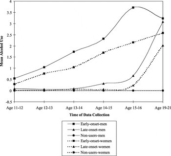
The alcohol use trajectories for men and women. For mean alcohol use, 0 = 0 glasses of alcohol in the past month, 1 = 1–2 glasses, 2 = 3–5 glasses, 3 = 6–9 glasses, and 4 = 10–19 glasses.
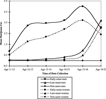
The marijuana use trajectories for men and women. For mean marijuana use, 0 = having smoked marijuana 0 times in the past year, 1 = 1–2 times, 2 = 3–5 times, 3 = 6–9 times, 4 = 10–19 times, 5 = 20–39 times, and 6 = 40+ times in the last year.
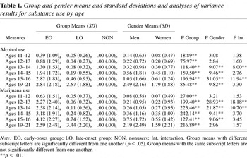
Group and gender means and standard deviations and analyses of variance results for substance use by age
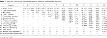
Bivariate correlations among and between predictor and outcome measures
Group and gender means and analyses of variance results for alcohol
Group and gender means and analyses of variance tesults for marijuana
 You have
Access
- 263
- Cited by