1. Introduction
The generation of micron-sized bubbles of controllable size at a desired frequency is an area of current active research as a consequence of the number of applications, such as ultrasound cleaning, sonoporation or ultrasound contrast imaging, that crucially depend on the use of these compressible objects (Ferrara, Pollard & Borden Reference Ferrara, Pollard and Borden2007; Rodríguez-Rodríguez et al. Reference Rodríguez-Rodríguez, Sevilla, Martínez-Bazán and Gordillo2015). The challenges imposed by the stringent demands of new technologies on both the sizes and the bubble formation frequencies are at the root of the progress in the design of new bubble makers. The improvements introduced in the new bubble generation methods are guided by the understanding of the dynamics of growth and collapse of bubbles, which notably differs from the well-known capillary mechanism leading to the disintegration of a continuous liquid stream (Rayleigh Reference Rayleigh1878), as is discussed at length in Rodríguez-Rodríguez et al. (Reference Rodríguez-Rodríguez, Sevilla, Martínez-Bazán and Gordillo2015). In chronological order, with the purpose of circumventing the problems associated with the production of bubbles by the direct injection of a gas stream into a stagnant liquid reservoir, Smith (Reference Smith1949), Chuang & Goldschmidt (Reference Chuang and Goldschmidt1970) and Og̃uz & Prosperetti (Reference Og̃uz and Prosperetti1993) placed the gas injection tube within an outer liquid coflow. This method possesses the advantages of (i) reducing the sizes of the bubbles produced, (ii) increasing the bubbling frequencies and (iii) avoiding the coalescence between neighbouring bubbles with respect to the case of bubble formation into a stagnant liquid pool. Subsequently, Gañán-Calvo & Gordillo (Reference Gañán-Calvo and Gordillo2001) and Garstecki et al. (Reference Garstecki, Gitlin, DiLuzio, Whitesides, Kumacheva and Stone2004) reported that the performance of the types of bubble generators resorting to the use of a liquid coflow could be further improved by directing the flow of liquid towards an orifice located in front of the gas injection tube, in a configuration termed, since then, flow focusing. Later on, Garstecki et al. (Reference Garstecki, Fuerstman, Stone and Whitesides2006) described the formation of microbubbles at the intersection of two perpendicular microchannels, in a geometrical arrangement that also possesses advantages with respect to the use of a coflowing liquid stream. An updated survey of the wealth of bubble production methods reported in the literature can be found in our recent review (Rodríguez-Rodríguez et al. Reference Rodríguez-Rodríguez, Sevilla, Martínez-Bazán and Gordillo2015).
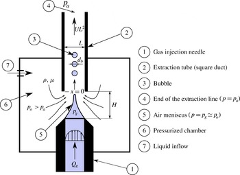
Sketch of the bubble production device operating in the regime of interest for applications, in which bubbles with very similar diameters
 $d_{b}$
are produced periodically at a frequency
 $f_{b}$
. Bubbles are emitted from the tip of a steady ligament attached to the exit of the injection needle, where the gas pressure
 $p_{g}$
is uniform in space. The origin of the dimensionless coordinate
 $x=X/L$
is located at the entrance of the square duct. The imposed gas flow rate is
 $Q_{g}$
and the extracted liquid flow rate is
 $UL^{2}$
.

It is our purpose in this paper to describe the critical role played by a favourable liquid pressure gradient in the periodic formation of microbubbles of controllable diameters
 $d_{b}$
at given frequencies
 $f_{b}$
. In our experimental study, we have made use of a geometrical arrangement that shares similarities with both the flow-focusing and the selective withdrawal geometries (Cohen et al.
Reference Cohen, Li, Hougland, Mrksich and Nagel2001; Gañán-Calvo & Gordillo Reference Gañán-Calvo and Gordillo2001) due to the fact that it allows for easy control of both the imposed pressure gradient and the gas flow rate. Our physical modelling provides closed expressions for both the bubbling frequencies and the bubble diameters which depend on whether the generation process is dominated by either liquid inertia or liquid viscosity.
The paper is structured as follows. In § 2 we describe the experimental observations, in § 3 the physical modelling is provided and in § 4 the conclusions are presented.
2. Phenomenology
In our experimental set-up, sketched in figure 1, the exit of a cylindrical needle of inner diameter 1.3 mm through which a flow rate
 $Q_{g}$
of air is injected is located at a distance
 $H$
from the entrance of a square extraction duct of width
 $L=1~\text{mm}$
; both the needle and the duct are aligned in the axial direction. Four liquids, with the material properties provided in table 1, are considered in this study. Therefore, since the ratio
 $h=H/L$
is fixed to either
 $h=1.15$
or
 $h=1.65$
, our experimental study consists of eight different data sets, two for each fluid. Both the injection needle and the extraction tube are immersed into a chamber filled with a liquid at a pressure
 $p_{0}>p_{a}$
, where
 $p_{a}$
is the atmospheric pressure at the end of the extraction duct (see
 $\unicode[STIX]{x2463}$
in figure 1). The imposed pressure difference
 $p_{0}-p_{a}$
fixes the mean liquid velocity
 $U$
in the square tube and also creates a pressure gradient from the exit of the injection needle towards the entrance of the extraction duct, favouring the stretching of the gas ligament downstream. The liquid flow rate,
 $UL^{2}$
, is calculated by measuring the volume of liquid exiting the pressurized chamber in a fixed interval of time. The gas flow rate is imposed by varying the gas pressure on one of the sides of the injection needle and the constancy of
 $Q_{g}$
during the bubble formation process is ensured by the large flow resistance of the injection line (Og̃uz & Prosperetti Reference Og̃uz and Prosperetti1993). Images are captured using a Phantom V7 high-speed camera which, depending on
 $U$
,
 $Q_{g}$
and
 ${\it\mu}$
, being
 ${\it\mu}$
the liquid viscosity, is operated between 1000 and 19 000 f.p.s.
Physical properties and characteristic values of the dimensionless groups characterizing the experiments performed with each of the four fluids used in this study. Here,
 ${\it\rho}$
,
 ${\it\mu}$
and
 ${\it\sigma}$
indicate the density, viscosity and interfacial tension of the liquid respectively,
 $\mathit{Re}={\it\rho}\,U\,L/{\it\mu}$
is the Reynolds number and
 $\mathit{We}={\it\rho}U^{2}L/{\it\sigma}$
is the Weber number. In order to lower the interfacial tension, SDS (sodium dodecyl sulphate) has been added to the water well above the critical micellar concentration. The rest of the liquids used are pure silicone oils.

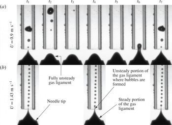
Figure 2 shows two possible regimes of bubble generation for a fixed value of the gas flow rate and increasing values of the mean liquid velocity. For the smaller values of
 $U$
, the air meniscus pulsates, emitting bubbles of unequal sizes. However, above a certain threshold, i.e. for
 $U>U^{\ast }$
, the gas ligament possesses a portion that remains steady along the spatial region
 $x\leqslant x_{s}$
, with the origin of the dimensionless coordinate
 $x=X/L$
located at the entrance of the extraction duct (see figure 1). Since the gas flow rate is kept constant during the bubble formation process and bubbles are produced periodically, the diameters of the bubbles generated for
 $U>U^{\ast }$
are, apparently, identical (see figure 3). This is the reason why the regime depicted in figures 2(b) and 3 will be referred to in the following as the monodisperse bubbling regime, MBR. Let us point out here that the periodicity in bubble generation in the aforementioned regime is not caused by any external forcing; instead, it will be shown below that it is a consequence of the imposed liquid pressure gradient. From now on, we will focus on the description of the MBR only, since this is precisely the regime of bubble production of interest for applications.
In (a),
 $U<U^{\ast }$
and the meniscus does not possess a steady portion. As a consequence of this, the bubble production is not regular. In contrast, for the same value of the gas flow rate but a larger liquid velocity, figure (b) shows that, for
 $U>U^{\ast }$
, the gas ligament is steady from the exit of the injection needle up to a point located slightly upstream the entrance of the extraction tube. In the case of (b), bubbles of very similar sizes are emitted periodically from the tip of the steady ligament, within the so-called monodisperse production regime, MBR. Here,
 ${\rm\Delta}t=t_{j}-t_{j-1}=0.0013~\text{s}$
,
 ${\it\mu}=1~\text{cP}$
,
 $Q_{g}=2.2\times 10^{-8}~\text{m}^{3}~\text{s}^{-1}$
.

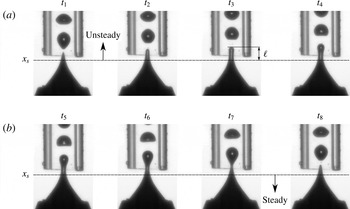
In the MBR, bubbles are produced from the tip of a steady air meniscus which extends from the exit of the injection needle down to
 $x_{s}$
. The snapshots corresponding to the instants of time
 $t_{1}$
and
 $t_{8}$
are practically identical, indicating that the bubble formation process is periodic. Once a bubble has been emitted, a new one grows from the gas thread of length
 $\ell$
extending downstream of
 $x_{s}$
. Here,
 ${\rm\Delta}t=t_{j}-t_{j-1}=5.2\times 10^{-5}~\text{s}$
,
 ${\it\mu}=1~\text{cP}$
,
 $U=1.38~\text{m}~\text{s}^{-1}$
,
 $Q_{g}=1.7\times 10^{-7}~\text{m}^{3}~\text{s}^{-1}$
.

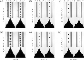
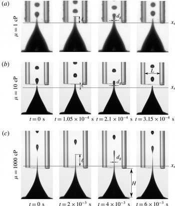
Figures 4 and 5 illustrate the bubbling processes within the MBR corresponding to three of the four liquids, of material properties provided in table 1, used in this study.
Images showing the bubble formation processes for liquids with three different viscosities. In all cases, both the bubble diameters and the bubbling frequencies can be controlled independently, by varying
 $Q_{g}$
and
 $U$
;
 $U$
is far smaller in the cases of liquids of higher viscosities.

Bubble formation process within the MBR for different viscosities. In (a,b), the interval between consecutive images,
 $t=1.05\times 10^{-4}~\text{s}$
, is identical for
 ${\it\mu}=1~\text{cP}$
and
 ${\it\mu}=10~\text{cP}$
. In (c),
 ${\it\mu}=1000~\text{cP}$
,
 $t=2\times 10^{-3}~\text{s}$
. The definitions of
 $\ell$
and
 $d_{g}$
, to be used in § 3, are also sketched. One can observe the dependence of
 $\ell$
on the liquid viscosity. In (a),
 $Q_{g}=4.3\times 10^{-8}~\text{m}^{3}~\text{s}^{-1}$
,
 $U=1.18~\text{m}~\text{s}^{-1}$
; in (b),
 $Q_{g}=2.75\times 10^{-8}~\text{m}^{3}~\text{s}^{-1}$
,
 $U=1.43~\text{m}~\text{s}^{-1}$
; in (c),
 $Q_{g}=5.9\times 10^{-10}~\text{m}^{3}~\text{s}^{-1}$
,
 $U=0.06~\text{m}~\text{s}^{-1}$
.

Figure 4 shows that, independently of the liquid viscosity, the diameters of the bubbles,
 $d_{b}$
, can be easily controlled by varying
 $U$
and
 $Q_{g}$
. Moreover, from this figure we note that, for the three values of
 ${\it\mu}$
considered in this figure,
 $d_{b}$
, which is notably smaller than
 $L$
, increases with
 $Q_{g}$
and decreases with
 $U$
. Figure 5 shows that the typical bubbling frequencies,
 $f_{b}$
, are smaller in the cases of the flows dominated by viscosity. Moreover, figures 3–5 reveal that, in the MBR, bubbles are produced downstream of the steady portion of the air meniscus. Indeed, figures 3 and 5 show that, right after the previous bubble has pinched off, the next one starts to grow from a cylindrical gas thread of diameter
 $d_{g}$
and length
 $\ell$
extending downstream of
 $x_{s}$
.
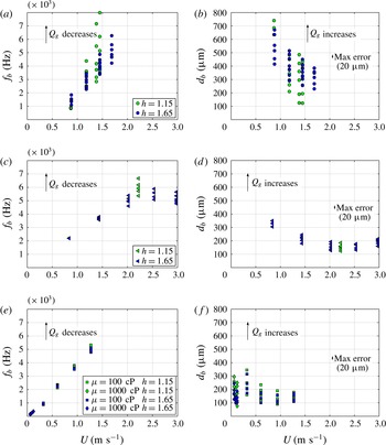
The dimensional values of
 $d_{b}$
and
 $f_{b}$
corresponding to all of the experimental data collected in this study are provided in figure 6. From figure 6, we observe that the bubbling frequencies increase monotonically with
 $U$
for the liquids with viscosities of 1, 100 and 1000 cP. However, for
 ${\it\mu}=10~\text{cP}$
, the variation of
 $f_{b}$
with
 $U$
is non-monotonic: it increases for values of
 $U$
between 1 and
 $2.5~\text{m}~\text{s}^{-1}$
and then decreases for higher values of the mean velocity. Moreover, while
 $f_{b}$
decreases when
 $Q_{g}$
increases for
 ${\it\mu}=1$
and
 ${\it\mu}=10~\text{cP}$
, the bubbling frequency is rather insensitive to variations of
 $Q_{g}$
for the liquids with viscosities of
 ${\it\mu}=100~\text{cP}$
and
 ${\it\mu}=1000~\text{cP}$
. Figure 6 reveals that, in all the experiments,
 $d_{b}$
increases with
 $Q_{g}$
and, in general, an increase of the mean velocity
 $U$
implies a decrease in
 $d_{b}$
. This latter trend is, again, broken in the case of the experiments with
 ${\it\mu}=10~\text{cP}$
and the largest mean velocities.
The measured frequencies
 $f_{b}$
(a,c,e) and the diameters of the bubbles generated
 $d_{b}$
(b,d,f) for the four liquids investigated in this study and for each of the two values of
 $h=H/L$
considered. The information is classified according to the liquid viscosity: (a,b),
 ${\it\mu}=1~\text{cP}$
, (c,d)
 ${\it\mu}=10~\text{cP}$
and (e,f)
 ${\it\mu}=100~\text{cP}$
,
 ${\it\mu}=1000~\text{cP}$
. The arrows indicate decreasing (a,c,e)/increasing (b,d,f) values of
 $Q_{g}$
. Two general trends are observed: (i) the bubbling frequencies increase for a fixed value of
 $U$
and decreasing values of
 $Q_{g}$
and (ii) the diameters of the bubbles increase for a fixed value of
 $U$
and increasing values of
 $Q_{g}$
. The bar in (b,d,f) indicates the maximum error in the measured value of
 $d_{b}$
. The analogous bar is not indicated in (a,c,e) since the errors associated with the measured values of
 $f_{b}$
are negligible.

3. Analysis
3.1. Necessary conditions for bubble production within the MBR
To determine the conditions under which monodisperse microbubbles are generated at a constant frequency in the MBR (see figures 3–5), we note first that, as is pointed out in Rodríguez-Rodríguez et al. (Reference Rodríguez-Rodríguez, Sevilla, Martínez-Bazán and Gordillo2015) and sketched in figure 1, the gas pressure within the air meniscus is uniform in space. The pressure
 $p_{g}$
can be determined from the normal stress balance at the exit of the gas injection needle, where both the capillary pressure and the modulus of the liquid velocity are negligible; consequently,
 $p_{g}\simeq p_{0}$
. The steadiness of the air meniscus along the spatial region
 $x\leqslant x_{s}$
, which is a necessary condition for bubbles to be produced within the MBR, is ensured while the pressure jump across the interface,
 $p_{0}-p(x)$
, is counterbalanced by the capillary pressure. Here,
 $p(x)$
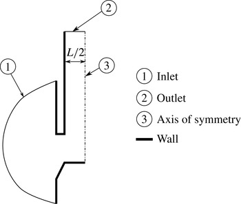
is a steady function calculated numerically at the axis of symmetry of the spatial domain sketched in figure 7 using a commercial code based on the volume of fluid method. Since the gas phase is not simulated, the calculated value of
 $p(x)$
refers to the unperturbed pressure described in Gordillo, Sevilla & Campo-Cortés (Reference Gordillo, Sevilla and Campo-Cortés2014):
 $p(x)$
is the pressure field associated with just the liquid flow satisfying the boundary conditions sketched in figure 7. Following the ideas in Gordillo et al. (Reference Gordillo, Sevilla and Campo-Cortés2014), the real liquid pressure at the interface could be expressed, in a first approximation, as the addition of the unperturbed pressure field, plus the perturbation caused by the gas jet. We neglect this subdominant contribution and the accuracy of the present approach will be verified a posteriori.
The Navier–Stokes equations are solved numerically in an axisymmetric domain since the extraction duct is approximated by a cylinder of radius
 $L/2$
. The equations are subjected to the no-slip boundary condition at the ‘wall’ boundaries. The modulus of the normal velocity imposed at the ‘inflow’ boundary is constant and such that the liquid flow rate is
 $UL^{2}$
.

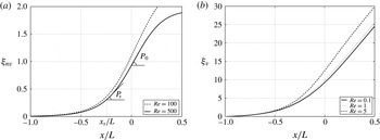
In figure 8, the values of the dimensionless functions
 ${\it\xi}_{nv}=(p_{0}-p(x))/(1/2{\it\rho}U^{2})$
and
 ${\it\xi}_{v}=(p_{0}-p(x))/({\it\mu}U/L)$
are represented for several values of the Reynolds number. As expected,
 $p_{0}-p(x=0)\simeq 1/2{\it\rho}U^{2}$
since
 ${\it\xi}_{nv}\simeq 1$
at
 $x\simeq 0$
in figure 8(a), a fact implying that the liquid velocity profile is uniform at the entrance of the square duct for
 $\mathit{Re}={\it\rho}UL/{\it\mu}\gg 1$
. In contrast, for
 $\mathit{Re}\leqslant 5$
,
 $\text{d}{\it\xi}_{v}/\text{d}x\simeq 32$
for
 $x\simeq 0$
or, equivalently,
 $\text{d}p/\text{d}X=-32{\it\mu}U/L^{2}$
, a fact implying that the velocity profile is parabolic right at the entrance of the extraction duct in the case of figure 8(b). Consequently, denoting by
 $U_{0}$
the liquid velocity at the axis of symmetry at
 $x\simeq 0$
, and in view of the range of operating Reynolds numbers shown in table 1,
 $U_{0}=U$
for the liquids with viscosities of
 ${\it\mu}=1~\text{cP}$
and
 ${\it\mu}=10~\text{cP}$
, and
 $U_{0}=2\,U$
for the liquids with viscosities of
 ${\it\mu}=100~\text{cP}$
and
 ${\it\mu}=1000~\text{cP}$
. The diameter
 $d_{g}$
of the gas ligament at
 $x_{s}$
(see figure 5) can now be approximated by means of the continuity equation
 $$\begin{eqnarray}Q_{g}\simeq \frac{{\rm\pi}d_{g}^{2}}{4}U_{0}\Rightarrow d_{g}\approx \left(\frac{Q_{g}}{U_{0}}\right)^{1/2},\end{eqnarray}$$
and, therefore, static equilibrium will be possible from the exit of the gas injection needle down to
 $x_{s}$
, with
 $x_{s}$
given by the solution of the equation
 $$\begin{eqnarray}p_{0}-p(x_{s})=\frac{2{\it\sigma}}{d_{g}}\simeq \frac{2{\it\sigma}}{(Q_{g}/U_{0})^{1/2}},\end{eqnarray}$$
with
 $p_{0}-p(x)$
provided in figure 8.
The dimensionless functions
 ${\it\xi}_{nv}(x)=(p_{0}-p(x))/(0.5{\it\rho}U^{2})$
(a) and
 ${\it\xi}_{v}(x)=(p_{0}\,-\,p(x))/({\it\mu}U/L)$
(b) represent the numerically calculated unperturbed pressure variations along the axis of symmetry for several values of the Reynolds number,
 $\mathit{Re}=100$
and
 $\mathit{Re}=500$
(a), and
 $\mathit{Re}=0.1$
,
 $\mathit{Re}=1$
and
 $\mathit{Re}=5$
(b). The solutions shown in (a) and (b) have been calculated numerically by means of commercial software based on the volume of fluid method which solves the Navier–Stokes equations subjected to the boundary conditions sketched in figure 7. The calculated results correspond to
 $h=1.65$
; the results obtained for
 $h=1.15$
are identical to those shown in this figure. In (a),
 $P_{s}$
indicates the slope of the function
 ${\it\xi}_{nv}$
at
 $x_{s}$
, namely
 $P_{s}=\dot{{\it\xi}}_{nv}(x_{s})$
, with
 $x_{s}$
the solution of the equation
 ${\it\rho}U^{2}/2{\it\xi}_{nv}(x_{s})=2{\it\sigma}/d_{g}$
. The particular values of
 $x_{s}$
and
 $P_{s}$
depicted in (a) correspond to the experimental conditions of figure 9(b).

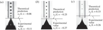
As is exemplified in figure 9, we have checked that the solution of (3.2) very closely predicts the experimental values of
 $x_{s}$
for the different liquids considered in this study. Clearly, the results illustrated in figure 9 validate the way in which the pressure field is approximated through the functions
 ${\it\xi}_{v}$
and
 ${\it\xi}_{nv}$
in figure 8. Next, making use of the experimental observation that
 $x_{s}\lesssim 0.5$
, we use (3.2) to deduce a necessary condition for bubbles to be generated within the MBR. Indeed,
 $p_{0}-p(x_{s})\sim 1/2{\it\rho}U^{2}$
for
 $\mathit{Re}\gg 1$
whereas
 $p_{0}\!-\!p(x_{s})\sim 32{\it\mu}U/L$
for
 $\mathit{Re}\lesssim 5$
(see figure 5). In addition, since (3.2) possesses a solution only when
 $p_{0}-p(x_{s})>2{\it\sigma}/d_{g}$
, the equations
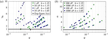
 $$\begin{eqnarray}{\it\beta}=\frac{{\it\rho}\,U^{2}\,L}{4{\it\sigma}}q^{1/2}\gtrsim 1\quad \text{and}\quad {\it\eta}=\frac{16}{\sqrt{2}}\frac{{\it\mu}\,U}{{\it\sigma}}q^{1/2}\gtrsim 1\quad \text{with}~q=\frac{Q_{g}}{UL^{2}}\,\end{eqnarray}$$
express the necessary conditions for bubbles to be produced in the MBR in the high (
 ${\it\beta}$
) and low to moderate (
 ${\it\eta}$
) Reynolds numbers respectively. The conditions given by (3.3) are tested in figure 10, where it is depicted that all the experimental data points lie within the regions
 ${\it\beta}\geqslant 1$
or
 ${\it\eta}\geqslant 1$
.
The comparison between the calculated value
 $x_{s}$
obtained from the solution of (3.2) and the observed one. Here, in (a),
 $Q_{g}=6.9\times 10^{-8}~\text{m}^{3}~\text{s}^{-1}$
,
 $U=0.88~\text{m}~\text{s}^{-1}$
; in (b),
 $Q_{g}=2.35\times 10^{-8}~\text{m}^{3}~\text{s}^{-1}$
,
 $U=1.43~\text{m}~\text{s}^{-1}$
; in (c),
 $Q_{g}=1.4\times 10^{-10}~\text{m}^{3}~\text{s}^{-1}$
,
 $U=0.06~\text{m}~\text{s}^{-1}$
. We have checked that, with independence of the liquid viscosity, the predicted values of
 $x_{s}$
are always very close to the measured ones ((a)
 ${\it\mu}=1~\text{cP}$
, (b) 10 cP and (c) 1000 cP).

All of the experimental data points corresponding to the conditions of bubble formation in the MBR satisfy the necessary conditions expressed by (3.3) in both the inertia dominated (a) and the viscous dominated regimes (b). The black square in (a),
 ${\it\beta}=0.84$
and
 $q=0.02$
, corresponds to the experimental conditions in figure 2(a). Since
 ${\it\beta}<1$
, the meniscus pulsates and the bubbles produced are not monodisperse.

3.2. Description of bubble generation within the MBR
Once a bubble detaches from the gas ligament, the pressure difference
 ${\rm\Delta}p=p_{0}-p(x)-2{\it\sigma}/d_{g}>0$
with
 $L\,x\approx L\,x_{s}+\ell$
induces radially outward velocities to the liquid surrounding the gas cylinder of length
 $\ell$
and diameter
 $d_{g}$
, beginning the formation of a new bubble (see figures 3 and 5). It should be noted that, during the instants following the detachment of the previous bubble, the diameter of the air cylinder hardly varies in time (see figures 3 and 5), and therefore
 $$\begin{eqnarray}\displaystyle {\rm\Delta}p & = & \displaystyle p_{0}-p(x)-\frac{2{\it\sigma}}{d_{g}}=p_{0}-p(x_{s})-\frac{2{\it\sigma}}{d_{g}}+p(x_{s})-p(x)\nonumber\\ \displaystyle & \simeq & \displaystyle -\frac{\text{d}p}{\text{d}x}(x_{s})(x-x_{s})\approx \frac{\text{d}(p_{0}-p)}{\text{d}x}(x_{s})\frac{\ell }{L},\end{eqnarray}$$
where the fact that
 $p_{0}-p(x_{s})-2{\it\sigma}/d_{g}=0$
has been taken into account. The result in (3.4) reveals that the growth and collapse of bubbles is forced by the local pressure gradient at
 $x_{s}$
, with
 $x_{s}$
the solution of (3.2). In fact, the local pressure gradient plays a role in the present physical situation that is similar to the one played by the gravitational acceleration in the formation of bubbles in a quiescent liquid pool. Indeed, we will check a posteriori that the process of bubble formation is locally dominated by inertia in the cases of
 ${\it\mu}=1~\text{cP}$
and
 ${\it\mu}=10~\text{cP}$
and by viscosity in the case of liquids of
 ${\it\mu}=100~\text{cP}$
and
 ${\it\mu}=1000~\text{cP}$
. Therefore, in order to scale the frequencies and diameters of the bubbles formed, we will make use of the momentum balances, inspired by the Rayleigh–Plesset equation (Og̃uz & Prosperetti Reference Og̃uz and Prosperetti1993; Rodríguez-Rodríguez et al.
Reference Rodríguez-Rodríguez, Sevilla, Martínez-Bazán and Gordillo2015),
 $$\begin{eqnarray}{\it\mu}=1,10~\text{cP}:\quad {\it\rho}R_{b}\ddot{R}_{b}\propto \frac{\text{d}(p_{0}-p)}{\text{d}x}(x_{s})\frac{\ell }{L}\propto \frac{\ell }{2\,L}{\it\rho}U^{2}P_{s},\end{eqnarray}$$
with
 $R_{b}$
indicating the time-dependent radius of the growing bubble,
 $P_{s}=\dot{{\it\xi}}_{nv}(x_{s})$
(see figure 8) and
 $$\begin{eqnarray}{\it\mu}=100,1000~\text{cP}:\quad 4{\it\mu}\frac{{\dot{R}}_{b}}{R_{b}}\propto \frac{d(p_{0}-p)}{\text{d}x}(x_{s})\frac{\ell }{L}\propto 32\frac{{\it\mu}U}{L^{2}}\ell .\end{eqnarray}$$
Equations (3.5)–(3.6) need to be complemented with the continuity equation
 $$\begin{eqnarray}Q_{g}=\frac{{\rm\pi}}{6}d_{b}^{3}\,f_{b}.\end{eqnarray}$$
It should be noted that (3.5)–(3.6) share many similarities with the momentum balances describing the formation of bubbles in a quiescent liquid pool (Rodríguez-Rodríguez et al.
Reference Rodríguez-Rodríguez, Sevilla, Martínez-Bazán and Gordillo2015), with the only difference being that the role played by the gravitational force per unit volume in that case,
 ${\it\rho}g$
, is substituted in the present one by the local pressure gradient which, however, is orders of magnitude larger,
 ${\it\rho}U^{2}/L\gg {\it\rho}\,g$
and
 $32{\it\mu}U/L^{2}\gg {\it\rho}g$
.
From (3.5) it can be deduced that, in the case of bubble generation dominated by inertia,
 $$\begin{eqnarray}{\it\rho}\frac{P_{s}}{2}\frac{U^{2}}{L}\ell \propto {\it\rho}R_{b}\ddot{R}_{b}\sim {\it\rho}d_{b}^{2}f_{b}^{2}\Rightarrow f_{b}\propto \frac{U\sqrt{P_{s}/2}}{\sqrt{L\,d_{b}}}\sqrt{\frac{\ell }{d_{b}}},\end{eqnarray}$$
and, analogously, in the viscous dominated case,
 $$\begin{eqnarray}32{\it\mu}\frac{U}{L^{2}}\,\ell \propto 4{\it\mu}\frac{{\dot{R}}_{b}}{R_{b}}\sim 4{\it\mu}f_{b}\Rightarrow f_{b}\propto 8\frac{U}{L^{2}}\ell .\end{eqnarray}$$
The analogy with the formation of bubbles in a quiescent liquid pool suggests that
 $\ell \propto d_{b}$
and, thus, the substitution of this result into (3.8) yields
 $$\begin{eqnarray}f_{b}\propto \frac{U\sqrt{P_{s}/2}}{\sqrt{L\,d_{b}}}\quad \text{and}\quad \frac{Q_{g}}{U\sqrt{P_{s}/2}}\sqrt{d_{b}L}\propto d_{b}^{3}\Rightarrow \frac{d_{b}}{L}\propto \left(\frac{Q_{g}}{U\sqrt{P_{s}/2}\,L^{2}}\right)^{2/5},\end{eqnarray}$$
where use of the mass balance (3.7) has been made. In (3.10), it should be noted that the expression for
 $d_{b}$
differs by the factor
 $\sqrt{P_{s}/2}$
from that in Gañán-Calvo (Reference Gañán-Calvo2004), where neither the corresponding expression for
 $f_{b}$
nor its comparison with experimental data was provided.
In the viscosity dominated cases, however, the characteristic axial length
 $\ell$
of the cylinder is no longer proportional to the bubble diameter
 $d_{b}$
. In fact, analysis of images of the type in figure 5 reveals that
 $\ell \propto L$
. This is so because the periodic bubbling regime described here is characterized by the fact that the gas ligament does not retract upstream once a bubble is formed. Indeed, at
 $x_{s}+\ell$
, the pressure drop is
 $32{\it\mu}U/L+32{\it\mu}U/L^{2}\ell$
, with
 $32{\it\mu}U/L\sim 2{\it\sigma}/d_{g}$
, and, moreover, once the bubble is detached, the capillary pressure corresponding to the spherical cap formed at
 $x_{s}+\ell$
is
 $4{\it\sigma}/d_{g}$
. Thus, since the gas pressure remains nearly uniform and equal to
 $p_{0}$
up to
 $x_{s}+\ell$
, the gas ligament will not retract if
 $$\begin{eqnarray}\frac{32\,{\it\mu}\,U}{L}+\frac{32\,{\it\mu}\,U}{L^{2}}\,\ell =\frac{4{\it\sigma}}{d_{g}}\Rightarrow \frac{32\,{\it\mu}\,U}{L^{2}}\,\ell \sim \frac{2{\it\sigma}}{d_{g}}=32{\it\mu}U/L\rightarrow \ell \simeq L.\end{eqnarray}$$
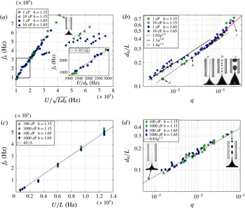
Panels (a) and (b) confirm the predictions in (3.10) for the case of
 ${\it\mu}=1~\text{cP}$
with
 $q\lesssim 0.1$
. For larger values of
 $q$
, the inset in (a) shows that
 $f_{b}\propto U/d_{b}$
, in agreement with (3.13), where it is also found that
 $d_{b}\propto q^{1/2}$
for
 $q\gtrsim 0.1$
(see figure 6
b). Moreover, panel (a) also shows a clear departure of the expected bubbling frequencies for most of the experimental data corresponding to
 ${\it\mu}=10~\text{cP}$
. The large differences in the bubbling frequencies observed between the cases of
 ${\it\mu}=1~\text{cP}$
and
 ${\it\mu}=10~\text{cP}$
in panel (a) correspond, however, to small but noticeable deviations from the expected bubble diameter given by (3.10), see panel (b). In fact, in the case of
 ${\it\mu}=10~\text{cP}$
, the experimental bubble diameters follow (3.14). Panels (c) and (d) confirm the predictions in (3.12).

Therefore, the substitution of
 $\ell =L$
into (3.9) together with the mass balance (3.7) yields
 $$\begin{eqnarray}f_{b}\propto 8\frac{U}{L}\quad \text{and}\quad \frac{Q_{g}\,L}{8\,U}\propto d_{b}^{3}\Rightarrow \frac{d_{b}}{L}\propto \left(\frac{Q_{g}}{U\,L^{2}}\right)^{1/3}.\end{eqnarray}$$
Figure 11 confirms the predictions of (3.10) for the case of
 ${\it\mu}=1~\text{cP}$
in the range of low to moderate values of
 $q$
and of (3.12) for the experiments in which the bubbling process is dominated by viscosity. However, the data corresponding to
 ${\it\mu}=1~\text{cP}$
and
 $q\gtrsim 0.1$
as well as those corresponding to
 ${\it\mu}=10~\text{cP}$
deviate from the scalings proposed in (3.10) and (3.12). It should be noted from figure 11 that, in the case of
 ${\it\mu}=1~\text{cP}$
, the experiments depart from the predicted behaviour for values of
 $q$
such that
 $d_{b}\sim 0.5L$
. In this case, the bubbles are so large that
 $\ell =L$
in (3.4) and, therefore,
 ${\rm\Delta}p\propto {\it\rho}U^{2}$
, a fact meaning that, in this case, the formation of bubbles is not triggered by the local pressure gradient, but by the global pressure drop
 $\propto {\it\rho}U^{2}$
. Therefore,
 $$\begin{eqnarray}{\it\rho}R_{b}\ddot{R}_{b}\sim {\it\rho}d_{b}^{2}\,f_{b}^{2}\propto {\it\rho}\,U^{2}\Rightarrow f_{b}\propto \frac{U}{d_{b}}\quad \text{and}\quad \frac{d_{b}}{L}\propto \left(\frac{Q_{g}}{U\,L^{2}}\right)^{1/2}\quad \text{for}~q\gtrsim 0.1,\end{eqnarray}$$
where use of the mass conservation (3.7) has been made. The results depicted in the inset of figure 11(a) as well as those for
 $d_{b}/L$
in the range
 $q\gtrsim 0.1$
shown in figure 11(b) validate the expressions provided in (3.13). It should be noted that (3.13) is deduced disregarding the apparent confinement effect that the extraction tube could exert on the formation of bubbles.
To understand the departure of the data corresponding to
 ${\it\mu}=10~\text{cP}$
with respect to the expected scalings, we note first from the horizontal axes in figure 11 that neither
 $f_{b}$
nor
 $d_{b}$
retains its dependence on
 $P_{s}$
predicted in (3.10). This is motivated by the fact that, in the case of water, the process of bubble generation takes place in a region
 $0\lesssim x_{s}+\ell <0.2$
, where
 $P_{s}$
is mostly constant and such that
 $P_{s}=P_{0}\simeq 3$
(see figure 8). However, figures 4 and 5 reveal that, in the case of
 ${\it\mu}=10~\text{cP}$
, bubbles begin to be formed upstream of the entrance of the extraction duct, at
 $x_{s}+\ell \lesssim 0$
, in a region where the values of
 $P_{s}$
suffer appreciable variations and where
 $P_{s}$
is notably smaller than
 $P_{0}$
, as is clearly shown in figure 8(a).
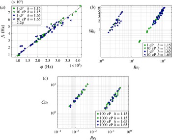
In addition, figure 12(b), where the values of the local Reynolds and Weber numbers defined in (3.15) are depicted, shows that the values of
 $Re_{l}$
are, in the cases of
 ${\it\mu}=10~\text{cP}$
, of order unity and thus appreciably smaller than in the cases of
 ${\it\mu}=1~\text{cP}$
. This fact explains the differences in the slenderness and the symmetry of the gas ligament at the pinch-off region depicted in figures 4 and 5. In addition, in the
 ${\it\mu}=10~\text{cP}$
case, viscosity contributes to smooth out the azimuthal perturbations present in the prompt pinch-off of bubbles generated in liquids with viscosities comparable to that of water. Thus, in the case of
 ${\it\mu}=10~\text{cP}$
, the minimum radius at which bubble pinch-off takes place is smaller than in the case of
 ${\it\mu}=1~\text{cP}$
(Keim et al.
Reference Keim, Moller, Zhang and Nagel2006; Bolaños-Jiménez et al.
Reference Bolaños-Jiménez, Sevilla, Martínez-Bazán and Gordillo2008; Gordillo Reference Gordillo2008). A direct consequence of all of these facts is that
 $\ell$
is shorter than
 $d_{b}$
in the case of
 ${\it\mu}=10$
cP, as figures 4 and 5 show. Guided by the experimental observations, we propose here that, for
 $Re_{l}<10$
,
 $\ell \propto d_{g}<d_{b}$
, with
 $Re_{l}$
the local Reynolds number defined in (3.15). The substitution of
 $\ell =d_{g}$
into (3.8), together with the mass conservation (3.7), yields
 $$\begin{eqnarray}f_{b}\propto \frac{U\sqrt{P_{s}/2}}{\sqrt{d_{b}\,L}}\left(\frac{d_{g}}{d_{b}}\right)^{1/2}\quad \text{and}\quad \frac{d_{b}}{L}\propto \left(\frac{P_{s}}{2}\right)^{-1/4}\left(\frac{Q_{g}}{U\,L^{2}}\right)^{3/8}.\end{eqnarray}$$
The results in figures 12 and 11(b) confirm the predictions in (3.14). It should be noted that the single multiplicative constant in
 $d_{b}/L\propto q^{3/8}$
in figure 11(b) results from the average values of
 $(P_{s}/2)^{-1/4}$
. To end the analysis of the experimental results we still need to verify our starting hypothesis, formulated at the beginning of this section, that bubble formation is dominated by inertia in the cases of
 ${\it\mu}\leqslant 10~\text{cP}$
and by viscosity for
 ${\it\mu}\geqslant 100~\text{cP}$
. For that purpose, figure 12(b) represents the values of both the local Weber and Reynolds numbers for the cases corresponding to the less viscous fluids. The values of these dimensionless parameters are respectively calculated as the ratios between the pressure difference
 $P_{0}/2{\it\rho}U^{2}/L\,d_{b}\simeq P_{0}/2{\it\rho}U^{2}q^{0.4}$
and either
 $2{\it\sigma}/d_{g}\simeq 2{\it\sigma}/Lq^{-0.5}$
or
 $4{\it\mu}{\dot{R}}_{b}/R_{b}\sim 4{\it\mu}f_{b}\sim 4{\it\mu}U\sqrt{P_{0}/2}/Lq^{-0.2}$
, namely
 $$\begin{eqnarray}\mathit{We}_{l}=(P_{0}/4)\,\mathit{We}q^{0.9},\quad \mathit{Re}_{l}=(\sqrt{P_{0}/2}/4)\,\mathit{Re}q^{0.6}.\end{eqnarray}$$
Analogously, in the case of bubble generation within the higher-viscosity liquids and, since in this case the characteristic pressure difference is
 ${\rm\Delta}p_{v}=32{\it\mu}U/L$
, the values of the local capillary and Reynolds numbers represented in figure 12(c) are respectively calculated as the ratio between
 ${\rm\Delta}p_{v}$
and
 $2{\it\sigma}/d_{g}$
(local capillary number) and as the ratio between
 ${\it\rho}{\dot{R}}_{b}^{2}\sim {\it\rho}d_{b}^{2}f_{b}^{2}\sim 16{\it\rho}U^{2}q^{2/3}$
and
 ${\rm\Delta}p_{v}$
(local Reynolds number), yielding
 $$\begin{eqnarray}\mathit{Ca}_{l}=\frac{16{\it\mu}\,U}{\sqrt{2}{\it\sigma}}q^{1/2}\quad \text{and}\quad \mathit{Re}_{l}=0.5\mathit{Re}\,q^{2/3}.\end{eqnarray}$$
Our initial hypothesis that bubble formation is dominated by liquid inertia in the cases of
 ${\it\mu}\leqslant 10~\text{cP}$
and by viscosity when
 ${\it\mu}\geqslant 100~\text{cP}$
is confirmed in view of the corresponding values of the local Reynolds numbers depicted in figure 12(b,c) and defined through (3.15)–(3.16).
Panel (a) shows that bubbling frequencies can be described in terms of a single function, linear in the parameter
 ${\it\phi}$
, with
 ${\it\phi}=U/\sqrt{Ld_{b}}$
if
 $\mathit{Re}_{l}>10$
and
 ${\it\phi}=U\sqrt{P_{s}/P_{0}}/\sqrt{d_{b}\,L}(d_{g}/d_{b})^{0.5}$
if
 $\mathit{Re}_{l}<10$
. Here,
 $P_{s}$
is the slope of the secant intersecting the curve
 ${\it\xi}_{nv}$
in figure 8 at the points
 $x_{s}$
and
 $x_{s}+d_{b}$
. Panel (b) provides the values of
 $\mathit{We}_{l}$
and
 $\mathit{Re}_{l}$
, defined in (3.15) for
 ${\it\mu}=1,~10~\text{cP}$
, whereas panel (c) shows the analogous values of
 $\mathit{Ca}_{l}$
and
 $\mathit{Re}_{l}$
, defined in (3.16) for
 ${\it\mu}=100,~1000~\text{cP}$
.

4. Conclusions
In this paper we have demonstrated the critical role played by the liquid pressure gradient in triggering the formation of monodisperse-sized microbubbles, finding the conditions for which the liquid pressure gradient induced production of bubbles is periodic for wide ranges of liquid viscosities. Moreover, we have provided the equations summarized in table 2 expressing both the bubbling frequencies
 $f_{b}$
and the bubble diameters
 $d_{b}$
as a function of the flow rate ratio
 $q=Q_{g}/(U\,L^{2})$
, the mean outer velocity
 $U$
and the width
 $L$
of the extraction tube. In the particular geometry considered here,
 $L$
is the characteristic length for which the liquid velocity in the pressurized chamber varies by of the order of the mean velocity in the square duct,
 $U$
. The agreement with the experimental data validates our physical modelling, which simply makes use of the gas mass conservation as well as the momentum equations (3.5)–(3.6), expressing that the local liquid pressure difference
 $-\partial p/\partial X(x_{s})\ell$
is balanced with either inertial or viscous stresses.
A summary of the main results in the paper. Here,
 $d_{g}=(Q_{g}/U)^{1/2}$
.

In spite of our study focusing on a particular type of geometrical arrangement, our main finding is that bubble formation is forced by the local pressure gradient. Therefore, the way in which the pressure gradients are created should not modify the expressions summarized in table 2. This is the reason why we believe that the ideas in this study could be used to guide the design of new types of bubble makers with geometries that may notably differ from the one presented here.
Acknowledgements
This work has been supported by the Spanish MINECO under Project DPI2014-59292-C3-2, partly financed through European funds.