


Introduction
Observations of the suspended-sediment load and dissolved-ion content of glacial outlet streams provide a valuable approach to studying the subglacial water system (Reference CollinsCollins, 1978, Reference Collins1979a, Reference Collinsb). Recently these techniques have been extended to in situ observations from instrumented boreholes (Reference StoneStone, 1993; Reference Stone, Clarke and BlakeStone and others, 1993; Reference Stone and Clarke.Stone and Clarke, in press). As yet, interpretation of these direct observations has been largely qualitative. In this paper I apply a lumped-element approach to simulate the responses of subglacial hydraulic, sediment and solute circuits. The merit of the lumped-element approximation is that it greatly simplifies otherwise complex Calculations, Although there is some sacrifice in mathematical rigour it is likely that the most serious limitation on subglacial hydrological models is poor knowledge of the drainage configuration, including solute and sediment sources, rather than oversimplification of the mathematical treatment.
Water Transport
A lumped-element formalism to describe subglacial hydraulic circuits was introduced at the International Workshop on Glacier Hydrology (Cambridge, U.K., 8–10 September 1993) and will be fully described elsewhere. Because water transport is an essential precondition for suspended-sediment and solute transport, I must introduce several hydraulic-circuit elements in order to develop simple water-discharge circuits capable of transporting sediment and solute. In addition to stating their mathematical attributes I propose schematic representations for each circuit clement (Fig. 1). These elements are respectively the crevasse input, square-law resistor, closed storage volume, single-pole double-throw (SPDT) switch and subaerial outlet. Viewed in isolation, each element is characterized by relationships between input and output values of hydraulic head (denoted h in and h out) and discharge (denoted Q in and Q out). When these elements are combined to form circuits, the governing equations commonly yield a differential-algebraic system. Such equations can be challenging to integrate, so special computational approaches must be applied (Reference Hairer, Lubich and RucheHairer and others, 1989; Reference Hairer and WannerHairer and Wanner, 1991).
Selected circuit elements for lumped-element modelling of water, sediment and solute discharge, (a) Circuit elements for hydrological circuit: A represents a crevasse input; B, a square-law resistor; C, closed storage; D, an SPDT switch; E, a subaerial outlet. (b) Circuit elements for solute and sediment exchange: A represents a resistor/exchanger; B, a storage/exchanger; Sed indicates sediment exchange; Ca indicates exchange of Ca2+ ions; other chemical species could also be added.

The crevasse input (A in Fig. 1a) is a combination of an ideal discharge source and a storage volume having the possibility of overflow when the volume is water-filled. If the volume is assumed to be straight-sided with base area A and overflow height h R the governing equation is

where h is the hydraulic head in the storage volume (measured relative to the base), Q in is the input discharge to the crevasse, and Q out is the output to the subglacial water system.
The square-law resistor (B in Fig. 1a) obeys the relations

where Q is the discharge through the resistor and R is a resistance coefficient. Calculation of R is based on the equations for turbulent pipe flow, Taking S as the cross-sectional area of the conduit, the cross-sectionally averaged flow velocity is v = Q/S, and the wall stress is given by τ 0 = f ρv 2/8 (e.g. Reference SchlichtingSchlichtung, 1979, p. 897) where f is the Darey–Weisbach friction Factor and ρ is the density of water. For a conduit of length l having wetted perimeter P, the balance of pressure forces acting on S and frictional drag acting on the pipe wall having area Pl gives ρg(h in - h out)S = Plτ 0, from which it follows that h in – h out = (fPl/8gS 3)Q 2 and R = fPl/8gS 3.
Closed storage (C in Fig. 1a) corresponds to a sealed water-storage volume within the glacier. For a vertical-walled reservoir having base area A V and maximum height h V the governing equations are

where the parameter 0 < A ε ≪ A V has been introduced to attenuate the discontinuity at h = h V. For suitably small values of A ε the equation dh/dt = (Q in – Q out)/A ε approximates the algebraic equation Q in = Q out and matches the circuit behaviour of a completely full storage volume.
The SPDT switch (D in Fig. 1a) allows the water-routing to be changed. If the input discharge to the switch is denoted Q in and at time t s the switch changes the routing from path A to path B the governing equations are


The last hydraulic element that I introduce is the subaerial outlet (E in Fig. 1a). This plays the simple rule of fixing the hydraulic head to zero. Thus, the governing equations are

General Balance Equation for Lumped Elements
In the lumped-element idealization, the exchange of sediment and solute to the water-discharge circuit is assumed to occur at specific sites rather than continuously along the water-flow path. Each of these sites is regarded as a “well-stirred reactor” so that spatial variation in the concentration of the reactor contents can be neglected. The general balance equation of continuum mechanics provides a useful starting-points for establishing the lumped-element forms of the sediment- and solute-balance equations. Suppose that z is the volume concentration of some extensive property Z within a region having volume V and bounded by a surface S. (To be specific, one might regard z as the mass of solute or suspended sediment per unit volume, and Z as the total mass of solute or suspended sediment within the reactor volume V). By definition
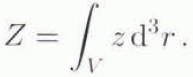
If the volume V varies temporally and substance flows into and out of V, then in general

where the first two righthand-side terms of Equation (7) respectively represent the convective and diffusive flux of z into the volume V, and the latter two terms represent the production and Supply of z within the volume. Convective flux of z occurs at the entry and exit ports of the reactor. If the surfaces that describe these ports are denoted S in and S out, respectively, then the discharge of Z across these surfaces is given by


In the cases where z is the concentration of suspended sediment or solute, diffusive flux occurs across the lower boundary surface A of the reactor, i.e. from the glacier bed, thus,

The basic assumptions of the lumped-element approximation are that z, ψ and a are spatially homogeneous in V and that  . n is homogeneous over A. Thus Equation (7) can be written

For subsequent work I shall assume that diffusion fluxes only occur across the bottom boundary surface A and that the supply term vanishes.
Suspended-Sediment Transport
Let c s denote the mass concentration of suspended sediment. Because the motivation for this work is to compare subglacial observations of sediment transport (and these are limited to optical turbidity measurements) I shall not concern myself with the bed-load component of sediment transport.
Erosion
For erosion of cohesionless sediment constructed of similar particles, Reference AllenAllen (1970, p. 52) suggests the relation

where E is the erosion rate, k E is a constant relating to the character of the flow and the bed surface. τ 0 is shear stress exerted by the flow onto its bed, τ* is a critical boundary shear stress that must be exceeded before erosion can proceed, and N is a constant determined from experiments; typically N ≈ 2. In the present work I assume that the supply of sediment is inexhaustible, but it would not be difficult to remove this assumption. For a permeable sediment substrate having porosity n and solid-phase density ρ s, the bed-normal mass flux of sediment from the bed into fluid suspension is

As has been noted, for turbulent flows the wall shear is written τ 0 = f ρv 2/8 where v = Q/S. The critical boundary stress depends on grain-size, and for extremely small particles such as silt τ* ≈ 0.
Sedimentation
I shall assume that Stokes’ law governs the sedimentation of suspended sediment. Thus,

is the settling velocity of spherical grains having diameter D p and density ρ s from a fluid of density ρ and viscosity μ. For a suspension of identical spherical grains, the bed-normal mass flux associated with sedimentation is therefore

As a matter of interest, the steady-state concentration  of suspended sediment can be calculated by setting
 and using Equations (13) and (15) to obtain

Sediment Balance
I now apply the lumped-element assumptions and take c
s as spatially constant within the volume V and  and
 as constant on the planar bed surface A. Sediment and water discharge are assumed to be fully coupled so that J
s
in = c
s
in
Q
in and J
s
out = c
s
out
Q
out where c
s
out = c
s. With these assumptions, Equations (11), (13) and (15) yield the sediment-balance equation

where V = Ah(t) for a vertical-walled container.
Solute Transport
Dissolution Kinetics
Let c i, denote the mass concentration of solute species i. In a sealed reactor that is well mixed, the solute concentration is spatially homogeneous and the chemical reaction equations for dissolution of constituent i can in many simple cases be written as

where S
i is the surface area of contact between solid and solution, k
i is the chemical reaction rate parameter, V is the volume of the chemical reactor, sgn denotes the algebraic sign function sgn(x) = x/|x|,  is the equilibrium concentration of constituent i, and v is the order of the chemical reaction (e.g. Reference WhiteWhite, 1988). Typically, k
i = k
0i exp(–Ei
/RT) where k
0i is a constant, Ei
is an activation energy, R is the gas constant and T is absolute temperature. Because the subglacial environment is nearly isothermal, temperature dependence of k
i will be neglected. Note that the dimensions of k
i depend on the value of v, but for any choice of v the term
 has dimensions kg m−3 s−1.
For simplicity I shall assume that the reactor can be treated as a straight-sided reservoir having base area A and height h(t). Thus, the reactor volume is

At the base of the reactor the surface area of contact between solid and solution is denoted S i, and I assume that

where F i is a form factor (related to the roughness of the reactor base. i.e. the glacier bed, as well as to the abundance of constituent i relative to other species). For a perfectly flat surface having a single mineralogy Fi = 1, but in Nature the value could be higher if the surface was rough, or lower if constituent i was weakly concentrated in the solid substrate. To illustrate the influence of surface roughness, suppose that the reactor base is viewed as a one-layer pavement of identical particles having diameter D p arranged to be in closest area packing; the area number density n A of particles forming this pavement is n A = 1/D p 2. Each particle has surface area S p = πD p 2, and if the entire particle surface is exposed to the solution then Fi = n A S p = π. If more than one layer was involved, Fi would take even larger values. Substituting Equations (19) and (20) into Equation (18) gives

Chemical Balance
In the spirit of the lumped-element approach, I assume that dissolution reactions proceed at specific sites beneath the glacier and that each of these sites can be represented by a continuous-flow stirred tank reactor. Thus, within the reactor the chemical concentrations are uniform but the inflowing and outflowing concentrations differ. The inflowing concentration of constituent i will be denoted ci in and the outflowing concentration is identical to that within the reactor so that ci out = ci . Solute discharge is assumed to be fully coupled to water discharge, thus Ji in = ci in Q in and Ji out = ciQ out. Chemical dissolution occurring at the basal boundary of the reactor can be represented as a diffusive discharge of constituent i across the area A and expressed as

Dissolution of constituent i from suspended sediment c s leads to volume-distributed production of constituent i within the reactor. If all suspended particles are identical spheres having diameter D p and density ρ s, then the mass of an individual particle is
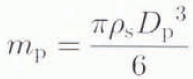
and the number density of suspended particle is

The surface area of an individual particle is S p = πD p 2 and the specific surface of suspended sediment is σ s = n s S p = 6c s/ρ s D p. From the chemical-reaction Equation (18), the rate of dissolution of constituent i from suspended sediment is therefore

Clearly, Equation (25) represents the volume-distributed chemical production of constituent i so that ψ i = (dc i/dt)s and from Equations (24) and (25)

Substituting Ji in = ci in Q in, Ji out = ciQ out and Equations (22) and (26) into Equation (11) gives

as the solute-balance equation. An interesting feature of Equation (27) is that it involves a three-way coupling between water transport (through Q in and Q out), sediment transport (through C s) and chemical transport.
Synthesis
The foregoing analysis illustrates that the lumped elements for sediment and solute exchange share common attributes with the previously defined flow-resistor and storage elements. For example, it is flow resistance (in the form of wall stress τ 0) that leads to sediment entertainment and a finite residence time (a property that implies water storage) that allows Stokes settling to proceed. Thus it is preferable to add sediment and solute exchange as attributes of the resistor and storage elements rather than introduce entirely new elements. These combination elements are referred to as the resistor/exchanger and storage/exchanger elements and are schematically depicted in Figure 1b.
The properties of resistor/exchanger elements are summarized by the following equations governing water, sediment and solute transport:


where Q = Q in = Q out, c s = c s out and c i = c i out. The resistance, area and volume appearing in Equations (28a) are assumed to describe a common drainage conduit. For simplicity this is assumed to have the geometry of a rectangular duct having dimensions ℓ (along-flow length), w (cross-flow width) and d (height), from which it immediately follows that A = wl is the base area, S = wd is the cross-sectional area and P = 2(w + d) is the perimeter of the conduit. Resistor/exchangers are assumed to be water-filled and to have constant volume; thus P corresponds to the wetted perimeter and dV/dt vanishes. For turbulent flow through the conduit, the wall stress is given by τ 0 = fρQ 2/8S 2, and the flow resistance coefficient is R = fPl/8gS 3.
The properties of the storage/exchanger elements are given by


The storage volume is assumed to have the geometry of a vertical-walled container with base area A v and temporally varying water volume V(t) = A v h(t). Water discharge through the storage volume is assumed to proceed sufficiently slowly that the substrate erosion term can be dropped from Equation (29b).
Simulation Example
Since summer 1989 the subglacial waler system of Trapridge Glacier (61°14′N, 140°20′W), Yukon Territory, Canada, has been subjected to continuous year-round measurements of subglacial water pressure, turbidity and electrical conductivity. The latter observations are proxies for subglacial suspended-sediment load and total dissolved-ion content. In the course of this measurement programme, occasional subglacial water-release events have been observed (Reference StoneStone, 1993: personal communication from C. C. Smart, 1986). I shall take the July 1990 release event, described by Reference StoneStone (1993), as the observational basis for this simulation example. Figure 2 shows measured water pressure, turbidity and electrical conductivity before and after the event. The event itself occurred at 2316 h on 22 July 1990 and is clearly indicated by a rapid increase in water turbidity (Fig. 2b). A noteworthy feature of the event is the change in character of the water-pressure signal (Fig. 2a); as recognized by Reference StoneStone (1993), prior to the event the water-pressure signal is quasi-exponential and following it the signal is quasi-sinusoidal. The event is marked by a rapid rise in turbidity (Fig. 2b) and a less rapid fall in electrical conductivity (Fig. 2c).
Subglacial water pressure, turbidity and electrical conductivity measurements from Trapridge Glacier, July 1990. Note the occurrence of a subglacial hydrological event at 2316 h on 22 July 1990.

Stone’s interpretation of the July 1990 release event is amply bolstered by observations that will not be discussed here. In outline, the event is thought to coincide with the establishment of an exit conduit for subglacial water. The formation of this conduit initiates flow in the subglacial water system and replaces mineralized subglacial water with unmineralized water routed from the glacier surface.
The lumped-element circuit that I introduce to emulate these features is shown in Figure 3. An essential feature of the circuit is the presence of the switch which diverts the water flow from a high-resistance path (through RX-2B) to a low-resistance path (through RX-2A). The storage/exchanger VX-1 has been included to enhance the tutorial value of this example. Its presence actually degrades the agreement between observations and model predictions, and for this reason I have chosen parameters that minimize the impact of VX-1 on the simulation results. The circuit nodes numbered 0, 1, 2 and 3 in Figure 3 denote points at which hydraulic head and discharge are evaluated. Values of the physical parameters of the model are summarized in Table 1 and specific values associated with individual circuit elements are presented in Table 2. Carbonate rocks are abundant in the vicinity of Trapridge Glacier, so for the simulation model I have thought of Ca2+ as the predominant cation. White (1988, p. 144) notes that for dissolution of CaCO3 it is found that v = 2 for many situations in Nature, so I have accepted this value in Table 1, The parameters D
p, n, τ*, N and Fi
have been assigned plausible values, and k
E,  , and ki
have been chosen to yield maximum sediment and solute concentrations in the range 1 kg m−3.
Proposed circuit to represent water, sediment and solute discharge before and after the July 1990 hydrological event. The onset of the event is initiated by throwing the switch from position B to position A.

Physical constants for simulation example

Parameter for lumped-element simulation example

The input forcings are assumed to be Q 0 = Q 0(t). c s0 = 0 and c 10 = 0. which corresponds to surface melt-water input containing no initial suspended sediment insolute. Noting that h 1 = h 2 the governing equations for the model are as follows:


where Θ(x) = sgn(x)|x|v, B
E = ρ
s( l – n)k
E and  . The switch position determines whether Q
2 passes through RX-2A or RX-2B and whether the parameters or RX-2A or RX-2B are used to calculate R
2, A
2, V
2 and τ
02 in Equations (33), (36) and (39).
Simulation results are given in Figure 4. Switching times and switch states are indicated by arrows and annotations along the upper frame boundary. In Figure 5 the interval from day 20 to day 26 is replotted to show details of the behaviour before and after the B ⟹ A switching event that releases stored subglacial water. Many qualitative features of the original data (Fig. 3) are reproduced. Before the switching event the hydraulic head shows no diurnal variation; following the event there is a sinusoidal diurnal signal. At the moment of the switching event the suspended-sediment load increases rapidly in association with increased subglacial water discharge. As a result of the increased discharge and reduced residence time of subglacial water the solute concentration drops dramatically. No attempt was made to optimize the selection of model parameters.
Simulated response of hydraulic circuit to switch-throwing. The switching times are indicated by arrows, and switch states by the letters A and B along the upper frame boundary. (a) Surface discharge (dashed line) into crevasse feeder and hydraulic head (solid line) at node 1 in Figure 3. (b) Suspended-sediment load at node 2 (solid line) and node 3 (dashed line) in Figure 3. (c) Solute concentration at node 1 (dotted line), node 2 (dashed line) and node 3 (solid line ) in Figure 3.

Detailed view of simulated response of hydraulic circuit to switch-throwing, the switching times are indicated by arrows, and switch states by the letters A and B along the upper frame boundary. (a) Surface discharge (dashed line) into crevasse feeder and hydraulic head (solid line) at node 1 in Figure 3. (b) Suspended-sediment load at node 2 (solid line) and node 3 (dashed line) in Figure 3. (e) Solute concentration at node 1 (dotted line), node 2 (dashed line) and node 3 (solid line) in Figure 3.

Concluding Remarks
Fruitful directions for future research would be to include more complex chemical relationships, for example the effect of dissolved CO2 on carbonate dissolution rate and to properly quantify the chemical rate constants. Inversion methods (e.g. Reference Murray and ClarkeMurray and Clarke, 1995) might be employed to estimate the parameters of simple circuits that optimally emulate observed records of hydraulic head, turbidity and electrical conductivity. As a first step it would be necessary to recast the lumped-element equations in dimensionless form in order to reduce the number of free parameters. Whether such an approach proves useful will in part depend upon the vigour of non-linearities in the hydraulic circuit. Lastly, computer models of ice-sheet dynamics are beginning to incorporate subglacial hydrology (e.g. Reference Arnold and SharpArnold and Sharp, 1992; Reference ArnoldArnold, 1993). Because the main purpose of such models is to promote understanding of the climate system it will soon become a priority to model the sediment and chemical fluxes from ice sheets. The lumped-element formalism described in this paper offers a comparatively simple starting-point.
Acknowledgements
This paper is a contribution to the Climate System History and Dynamics Programme (CSHD) that is jointly sponsored by the Natural Sciences and Engineering Research Council of Canada (NSERC) and the Atmospheric Environment Service of Canada. I wish to thank Professor E. Hairer of the Université de Genève for giving me a copy of his excellent but out-of-print book on differential-algebraic systems. Data collection on Trapridge Glacier was supported by an operating grant from NSERC; the theory and modelling by an NSERC collaborative grant. I thank Parks Canada and the Government of the Yukon for permission to conduct field-work in Kluane National Park.



