1. Introduction
Vortices of widely varying sizes exist in the Earth’s atmosphere and oceans, as well as in other planetary atmospheres. From synoptic-scale tropical cyclones to mesoscale Gulf Stream Rings and submesoscales eddies in the upper ocean, the structure and behaviour of these ‘geophysical’ vortices are strongly influenced by both the stable vertical density stratification and the planetary rotation. Vortices affect the collective motion of the atmosphere and the oceans and hence play an important role in our climate system. For example, anticyclonic mesoscale lens-shaped vortices called ‘meddies’ (McDowell & Rossby Reference McDowell and Rossby1978) found in the Gulf of Cadiz are thought to contribute significantly to the transport of heat and salinity into the North Atlantic Ocean. Geophysical vortices can often exist and evolve over long periods of time with minimal interaction with other coherent structures that may exist in the flow (Carton Reference Carton and Flor2010). A primary question then is why vortices exist and persist for many internal rotation periods, even when the background flow provides continuous disturbances. To address this, a natural starting point is to consider an isolated vortex, and determine how its shape and its strength affect its stability. While this approach is simplistic, we argue that it is relevant to the way in which vortices lose stability after being critically distorted by a background flow.
The study of isolated vortical structures, vortices, dates back to Rankine and Kirchhoff in the 19th century. The circular Rankine vortex (Rankine Reference Rankine1858) and the elliptical Kirchhoff vortex (Kirchhoff Reference Kirchhoff1876; Lamb Reference Lamb1932) are exact, shape-preserving solutions to the two-dimensional Euler equations for patches of uniform vorticity embedded in an unbounded potential flow. Extensions to include an ambient strain and shear flow were made by Chaplygin (Meleshko & van Heijst Reference Meleshko and van Heijst1994), Moore & Saffman (Reference Moore and Saffman1971) and Kida (Reference Kida1981), and stability was investigated by Dritschel (Reference Dritschel1990) and Meacham, Flirel & Send (Reference Meacham, Flirel and Send1990). For a review of early works on two-dimensional vortex dynamics, see Meleshko & van Heijst (Reference Meleshko and van Heijst1994).
In the more general geophysical context, isolated vortices called ‘rodons’ (Cushman-Roisin, Heil & Nof Reference Cushman-Roisin, Heil and Nof1985; Young Reference Young1986) have been found as exact solutions to the single-layer shallow-water equations (having a variable fluid depth), a model of warm-core rings shed by the Gulf Stream. Płotka & Dritschel (Reference Płotka and Dritschel2012) examined a wide class of vortex-patch equilibria with uniform potential vorticity (PV) in the quasi-geostrophic (QG) shallow-water equations, determining both their equilibrium shapes and stability numerically. Płotka & Dritschel (Reference Płotka and Dritschel2014) generalised this class to finite Rossby number, i.e. to the full shallow-water equations, and introduced the concept of ‘quasi-equilibria’: vortex solutions which steadily rotate apart from exceptionally weak gravity wave radiation. These are almost shape-preserving.
Some generalisations to three-dimensional rotating continuously stratified flows were made by Zhmur & Shchepetkin (Reference Zhmur and Shchepetkin1991) and Meacham (Reference Meacham1992), exploiting simplifications afforded by the QG approximation. They considered ellipsoidal volumes of uniform PV embedded in an otherwise quiescent unbounded fluid. Meacham (Reference Meacham1992) showed that such QG ellipsoidal vortices are steadily rotating shape-preserving solutions, hereafter ‘equilibria’. Moreover, Meacham (Reference Meacham1992) found that many vortices are linearly stable if close to a spherical form in the vertically stretched coordinate system
 $(x,y,Nz/f)$
where
 $f$
and
 $N$
are the Coriolis and buoyancy frequencies respectively. This coordinate system is a natural one for QG flows. Using a complementary approach, Dritschel, Scott & Reinaud (Reference Dritschel, Scott and Reinaud2005) found that these vortices are in fact stable over a much wider parameter range and furthermore examined their nonlinear stability and long-time evolution.
Meacham et al. (Reference Meacham, Pankratov, Shchepetkin and Zhmur1994) further generalised the ellipsoidal model to include a uniform background horizontal and vertical shear. Meacham, Morrison & Flirel (Reference Meacham, Morrison and Flirel1997) showed that the time-dependent vortex motion (which is potentially chaotic) can be described exactly in terms of a finite degree-of-freedom model obtained from the method of ‘Hamiltonian moment reduction’. The stability of QG ellipsoidal vortices has been studied for some special background flows, e.g. a pure horizontal strain flow (Meacham et al. Reference Meacham, Pankratov, Shchepetkin and Zhmur1994) and a pure shear flow for which the strain rate equals the background rotation (Hashimoto, Shimonishi & Miyazaki Reference Hashimoto, Shimonishi and Miyazaki1999). McKiver & Dritschel (Reference McKiver and Dritschel2006) studied the combined effects of horizontal strain and vertical shear on QG ellipsoidal vortices, analysing their linear stability to both ellipsoidal and non-ellipsoidal disturbances. Additional solutions to the QG equations representing a tilted spheroid rotating steadily about the vertical axis were discovered by Miyazaki, Ueno & Shimonishi (Reference Miyazaki, Ueno and Shimonishi1999), who also investigated their linear stability.
In a strongly stratified and rapidly rotating flow (having small Froude and Rossby numbers) there is a time-scale separation between the fast inertia–gravity waves (IGWs) and the slow ‘balanced’ vortical motions. This motivates the use of simplified balanced models – reduced models which filter out IGWs – for studying the slow PV-controlled dynamics (see Ford, McIntyre & Norton Reference Ford, McIntyre and Norton2000 and references therein). There is a direct analogue here to filtering sound waves by making the incompressible flow approximation. One of the simplest such balanced models, obtained in the limit of zero Rossby and Froude number (keeping an
 $O(1)$
ratio), is the QG model (Charney Reference Charney1948; Salmon Reference Salmon1998; Vallis Reference Vallis2006). In this model, the fluid motion and perturbation density field are entirely controlled by a single scalar quantity, the QG potential vorticity. This results in a major simplification of the original governing equations: one scalar field determines every aspect of the dynamics, the induced flow depends linearly on PV, and the system evolves at a slow rate proportional to the maximum PV, which is conserved in an adiabatic, frictionless flow. This may seem almost trivial, but what remains is nonlinear PV advection: PV induces the very flow which modifies its distribution. This can lead to complex, turbulent motion, albeit in a layerwise, two-dimensional sense.
Despite its broad applicability, the QG model is a balanced model of the lowest order and inevitably has its limitations. There are situations where departures from the QG limit are significant. For example, many mesoscale ocean eddies (Chelton, Schlax & Samelson Reference Chelton, Schlax and Samelson2011), including cyclonic and anticyclonic rings detached from major ocean currents (Olson Reference Olson1991; Lentini, Goni & Olson Reference Lentini, Goni and Olson2006) and meddies (Prater & Sanford Reference Prater and Sanford1994; Paillet et al.
Reference Paillet, Le Cann, Carton, Morel and Serpette2002), can have moderate Rossby numbers in the range of 0.1–1. Submesoscale eddies in the Southern California Bight tend to be ageostrophic with
 $O(1)$
Rossby numbers (Kim Reference Kim2010). Under these conditions, it has been shown that geophysical flows spontaneously emit IGWs during their evolution (Ford et al.
Reference Ford, McIntyre and Norton2000; Viúdez Reference Viúdez2007; Ólafsdóttir, Olde Daalhuis & Vanneste Reference Ólafsdóttir, Olde Daalhuis and Vanneste2008), indicating the non-existence of a strictly balanced system. Moreover, the QG model fails to distinguish between cyclonic and anticyclonic motions, due to the fact that the QG flow fields are linearly related to PV.
To better understand vortex dynamics in naturally occurring geophysical flows, there is a compelling need to go beyond our predominantly QG-based understanding. Specifically, we seek to answer key questions impacting on the validity of the QG approximation. How do ageostrophic effects change the stability and long-time evolution of a vortex? What role is played by IGWs? For how long can we expect a balanced model to faithfully represent vortex dynamics within a more complete model containing IGWs and higher-order ageostrophic effects? It is noteworthy that these questions are relevant to many practical applications in dynamical meteorology where the concept of balance is central to the understanding of large-scale vortical flows.
In this paper, we consider an incompressible stratified fluid in a three-dimensional rotating domain. For practical reasons, we are restricted to consider a finite domain, here triply periodic. Following many previous studies and to retain some simplicity, both the Coriolis and the buoyancy frequencies
 $f$
and
 $N$
are taken to be constant. Moreover, the Boussinesq approximation is employed. However, we do not assume hydrostatic balance nor geostrophic balance.
We study arguably the simplest vortex form possible, namely an ellipsoidal volume of uniform PV (or PV anomaly relative to a constant background). While in the QG model described above there are exact solutions for steadily rotating ellipsoidal vortices, no analogous solutions are known to exist for the non-hydrostatic Boussinesq equations. Instead we generate ‘quasi-equilibria’ by a novel numerical PV ramping procedure which spins up a non-hydrostatic ageostrophic flow with minimal excitation of IGWs. The solutions thus obtained are remarkably close to an ellipsoid shape. They are not strictly in equilibrium, in any frame of reference, due to the weak emission of IGWs occurring for any non-symmetric vortex shape. However, the emission is so weak that we may regard the solutions as equilibria and sensibly investigate their stability and long-time nonlinear evolution.
The problem investigated is governed by four parameters:
 $f/N$
, the PV-based Rossby number
 $q_{0}$
, the initial horizontal aspect ratio
 ${\it\lambda}_{0}$
and the initial vertical aspect ratio
 ${\it\mu}_{0}$
. When
 $f/N\ll 1$
, the dependence on
 $f/N$
is negligible (Smyth & McWilliams Reference Smyth and McWilliams1998; Dritschel & McKiver Reference Dritschel and McKiver2014), allowing us to focus attention on the remaining three parameters. We mention that the linear stability of an axisymmetric columnar vortex in a non-hydrostatic Boussinesq fluid has been studied by Smyth & McWilliams (Reference Smyth and McWilliams1998), but this lies outside the parameter space investigated here.
In § 2, the equations of motion are recast into a form suitable for flows that are close to a state of balance. We then discuss the numerical method and initialisation procedure employed. In § 3, we follow the nonlinear evolution of the vortex using an equivalent oriented ellipsoid. Phase diagrams are constructed identifying the stability boundary and categorising the long-time near-equilibrium state in terms of the vortex PV anomaly or Rossby number
 $q_{0}$
, and the initial vortex shape
 ${\it\lambda}_{0}$
and
 ${\it\mu}_{0}$
. Section 4 discusses the vortex rotation rate, specifically its correlation with the vortex shape, and the asymmetric role played by ageostrophic effects on cyclones and anticyclones. Section 5 analyses the structure and significance of balanced and imbalanced motions. The balanced flow is separated into a QG part and a remaining higher-order ageostrophic one, to clarify the impact of ageostrophic effects on vortex stability. The imbalanced flow is shown to take the form of radiating IGWs, albeit of very small amplitude across the entire parameter space. Finally, a few conclusions and suggestions for future study are provided in § 6.
2. Mathematical model and numerical method
2.1. Non-hydrostatic Boussinesq equations
We consider a rotating incompressible fluid with velocity
 $\boldsymbol{u}=(u,v,w)$
under the
 $f$
-plane approximation. With
 $z$
the vertical coordinate (normal to a reference geopotential surface), the fluid density
 ${\it\rho}$
and pressure
 $p$
are written as
 $$\begin{eqnarray}\displaystyle {\it\rho}(\boldsymbol{x},t) & = & \displaystyle {\it\rho}_{0}+\bar{{\it\rho}}(z)+{\it\rho}^{\prime }(\boldsymbol{x},t),\end{eqnarray}$$
 $$\begin{eqnarray}\displaystyle p(\boldsymbol{x},t) & = & \displaystyle \bar{p}(z)+p^{\prime }(\boldsymbol{x},t),\end{eqnarray}$$
 ${\it\rho}_{0}$
is a constant reference density. The basic-state quantities
 ${\it\rho}_{0}+\bar{{\it\rho}}$
and
 $\bar{p}$
satisfy hydrostatic balance
 $$\begin{eqnarray}\frac{\text{d}\bar{p}}{\text{d}z}=-({\it\rho}_{0}+\bar{{\it\rho}})g,\end{eqnarray}$$
where both the gravitational and centrifugal force contribute to the constant
 $g$
(Salmon Reference Salmon1998). The perturbation buoyancy
 $b$
and the buoyancy frequency
 $N$
are then defined through
 $$\begin{eqnarray}\displaystyle & \displaystyle b=-g\,{\it\rho}^{\prime }/{\it\rho}_{0}, & \displaystyle\end{eqnarray}$$
 $$\begin{eqnarray}\displaystyle & \displaystyle N^{2}=-\frac{g}{{\it\rho}_{0}}\frac{\text{d}\bar{{\it\rho}}}{\text{d}z}. & \displaystyle\end{eqnarray}$$
 $N$
to be constant, corresponding to a linear basic-state density profile.
Making the Boussinesq approximation (
 $\bar{{\it\rho}}$
,
 ${\it\rho}^{\prime }\ll {\it\rho}_{0}$
), the equations of motion may be simplified to
 $$\begin{eqnarray}\displaystyle & \displaystyle \frac{\text{D}\boldsymbol{u}}{\text{D}t}+f\,\hat{\boldsymbol{k}}\times \boldsymbol{u}=-{\it\rho}_{0}^{-1}\boldsymbol{{\rm\nabla}}p^{\prime }+b\,\hat{\boldsymbol{k}}, & \displaystyle\end{eqnarray}$$
 $$\begin{eqnarray}\displaystyle & \displaystyle \frac{\text{D}b}{\text{D}t}+N^{2}w=0, & \displaystyle\end{eqnarray}$$
 $$\begin{eqnarray}\displaystyle & \displaystyle \boldsymbol{{\rm\nabla}}\boldsymbol{\cdot }\boldsymbol{u}=0, & \displaystyle\end{eqnarray}$$
 $\text{D}/\text{D}t$
is the material derivative,
 $\hat{\boldsymbol{k}}$
is the unit vector in the
 $z$
-direction and
 $f$
is the Coriolis frequency (twice the constant background rotation rate).
2.2. Potential vorticity and ageostrophic vorticity
Following Dritschel & Viúdez (Reference Dritschel and Viúdez2003), we reformulate (2.6) using a set of variables that makes explicit the leading-order hydrostatic–geostrophic balance at small Rossby number. To this end, let us define the dimensionless total PV
 $Q$
and PV anomaly
 $q$
as
 $$\begin{eqnarray}Q=1+q=\frac{1}{f}\left({\bf\omega}+f\hat{\boldsymbol{k}}\right)\boldsymbol{\cdot }\boldsymbol{{\rm\nabla}}\left(\frac{b}{N^{2}}+z\right),\end{eqnarray}$$
where the vorticity
 ${\bf\omega}=({\bf\omega}_{h},{\it\zeta})=\boldsymbol{{\rm\nabla}}\times \boldsymbol{u}$
. The expression in the second bracket above is the isopycnal height. It is related to the density through
 $b/N^{2}+z=(1-{\it\rho}/{\it\rho}_{0})g/N^{2}$
. Hence,
 $Q$
is essentially the component of the absolute vorticity
 ${\bf\omega}+f\hat{\boldsymbol{k}}$
along the density gradient, normalised by
 $f$
. The basic state,
 ${\bf\omega}=b=0$
, then has
 $Q=1$
and
 $q=0$
.
A natural choice for the Rossby number is the PV anomaly
 $q$
itself, specifically its extreme value. Material conservation of PV implies that this Rossby number is constant. Its relation to the traditional Rossby number
 $U/f\,L$
may be seen by non-dimensionalising variables using QG scaling, i.e.
 $(x,y)=L(\tilde{x},{\tilde{y}})$
,
 $z=H\tilde{z}$
,
 $t=(L/U)\tilde{t}$
,
 $(u,v)=U({\tilde{u}},\tilde{v})$
,
 $w=(U/f\,L)(H/L)U\tilde{w}$
and
 $b=(U/f\,L)N^{2}H\tilde{b}$
, where
 $L$
and
 $H$
are typical horizontal and vertical length scales respectively, and
 $U$
is a typical horizontal velocity scale. Then the PV may be written
 $$\begin{eqnarray}Q=1+\frac{U}{f\,L}\biggl(\frac{\partial \tilde{b}}{\partial \tilde{z}}+\tilde{{\it\zeta}}\biggr)+\biggl(\frac{U}{f\,L}\biggr)^{2}\tilde{{\bf\omega}}\boldsymbol{\cdot }\tilde{\boldsymbol{{\rm\nabla}}}\tilde{b}.\end{eqnarray}$$
The non-dimensional variables, with tildes, are of
 $O(1)$
. Hence, to leading order the PV anomaly
 $q$
is just the traditional Rossby number. The extreme value of
 $q$
is a better choice as it does not require ad hoc choices for
 $U$
and
 $L$
.
The PV alone, however, is not sufficient to describe the dynamics of the flow, since the original system (2.6) has three independent time derivatives, after taking into account incompressibility. Motivated by QG balance, two additional variables are chosen from the horizontal (vector) component of the dimensionless ageostrophic (and non-hydrostatic) vorticity
 $$\begin{eqnarray}\boldsymbol{A}\equiv \frac{{\bf\omega}}{f}+\frac{\boldsymbol{{\rm\nabla}}b}{f^{2}}.\end{eqnarray}$$
Notably, the horizontal component
 $\boldsymbol{A}_{h}=0$
for a flow in thermal wind balance (apart from often negligible contributions from horizontal derivatives of the vertical velocity). Therefore,
 $\boldsymbol{A}_{h}$
captures higher-order ageostrophic motions beyond the leading-order hydrostatic–geostrophic balance. These motions include inertia–gravity waves, but are typically dominated by higher-order balance effects (Dritschel & Viúdez Reference Dritschel and Viúdez2007).
2.3. Reformulation of the governing equations
Instead of
 $\{\boldsymbol{u},b,p\}$
, we shall use
 $\{q,\boldsymbol{A}_{h}\}$
as the prognostic variables to explicitly enforce material conservation of PV. This enables a more accurate representation of both the balanced PV-controlled dynamics as well as the residual imbalance (Dritschel & Viúdez Reference Dritschel and Viúdez2003, Reference Dritschel and Viúdez2007). The equations of motion for
 $q$
and
 $\boldsymbol{A}_{h}$
are
 $$\begin{eqnarray}\displaystyle & \displaystyle \frac{\text{D}q}{\text{D}t}=0, & \displaystyle\end{eqnarray}$$
 $$\begin{eqnarray}\displaystyle & \displaystyle \frac{\text{D}\boldsymbol{A}_{h}}{\text{D}t}+f\hat{\boldsymbol{k}}\times \boldsymbol{A}_{h}=\frac{1}{f}({\bf\omega}\boldsymbol{\cdot }\boldsymbol{{\rm\nabla}})\boldsymbol{u}_{h}+(1-{\it\sigma}^{-2})\boldsymbol{{\rm\nabla}}_{h}w-\frac{1}{f^{2}}(\boldsymbol{{\rm\nabla}}_{h}\boldsymbol{u})\boldsymbol{\cdot }\boldsymbol{{\rm\nabla}}b, & \displaystyle\end{eqnarray}$$
 $\boldsymbol{u}_{h}$
is the horizontal velocity,
 $\boldsymbol{{\rm\nabla}}_{h}$
is the horizontal gradient operator and the dimensionless parameter
 $$\begin{eqnarray}{\it\sigma}\equiv \frac{f}{N}.\end{eqnarray}$$
We set
 ${\it\sigma}=0.1$
(a typical value for the oceans) for all the results reported here. The results are not sensitive to this parameter so long as
 ${\it\sigma}\lesssim 1$
(Dritschel & McKiver Reference Dritschel and McKiver2014).
The fields
 $\boldsymbol{u}$
and
 $b$
can be recovered from
 $\{q,\boldsymbol{A}_{h}\}$
as follows. Expressing
 $\boldsymbol{A}$
in terms of a potential
 ${\bf\varphi}$
,
 $$\begin{eqnarray}\boldsymbol{A}={\rm\nabla}^{2}{\bf\varphi},\end{eqnarray}$$
we have from (2.9),
 $$\begin{eqnarray}\displaystyle & \displaystyle \boldsymbol{u}=-f\,\boldsymbol{{\rm\nabla}}\times {\bf\varphi}, & \displaystyle\end{eqnarray}$$
 $$\begin{eqnarray}\displaystyle & \displaystyle b=f^{2}\,\boldsymbol{{\rm\nabla}}\boldsymbol{\cdot }{\bf\varphi}. & \displaystyle\end{eqnarray}$$
 ${\bf\varphi}_{h}$
and the vertical component
 ${\it\phi}$
of the potential
 ${\bf\varphi}$
are obtained from
 $\{q,\boldsymbol{A}_{h}\}$
by inverting the following relations:
 $$\begin{eqnarray}\displaystyle & \boldsymbol{A}_{h}={\rm\nabla}^{2}{\bf\varphi}_{h}, & \displaystyle\end{eqnarray}$$
 $$\begin{eqnarray}\displaystyle & \displaystyle q=\left({\rm\nabla}_{h}^{2}+{\it\sigma}^{2}\frac{\partial ^{2}}{\partial z^{2}}\right){\it\phi}-(1-{\it\sigma}^{2})\boldsymbol{{\rm\nabla}}_{h}\boldsymbol{\cdot }\frac{\partial {\bf\varphi}_{h}}{\partial z}+{\it\sigma}^{2}\boldsymbol{{\rm\nabla}}(\boldsymbol{{\rm\nabla}}\boldsymbol{\cdot }{\bf\varphi})\boldsymbol{\cdot }[{\rm\nabla}^{2}{\bf\varphi}-\boldsymbol{{\rm\nabla}}(\boldsymbol{{\rm\nabla}}\boldsymbol{\cdot }{\bf\varphi})].\qquad & \displaystyle\end{eqnarray}$$
 ${\bf\varphi}_{h}$
is known by solving the linear elliptic equation (2.15), we can rewrite (2.16) as a double Monge–Ampère equation in the unknown
 ${\it\phi}$
,
 $$\begin{eqnarray}{\it\sigma}^{2}({\it\phi}_{zz}{\rm\nabla}_{h}^{2}{\it\phi}-{\it\phi}_{xz}^{2}-{\it\phi}_{yz}^{2})+B_{1}{\rm\nabla}_{h}^{2}{\it\phi}+B_{2}{\it\phi}_{zz}+C_{1}{\it\phi}_{xz}+C_{2}{\it\phi}_{yz}+D=0,\end{eqnarray}$$
with the coefficients
 $B_{1}$
,
 $B_{2}$
,
 $C_{1}$
,
 $C_{2}$
and
 $D$
depending on
 ${\it\sigma}$
,
 ${\bf\varphi}_{h}$
and
 $q$
.
2.4. The contour-advective semi-Lagrangian algorithm and near-balanced initialisation
We solve the prognostic equations (2.10) numerically in a triply periodic box of horizontal side lengths
 $2{\rm\pi}L{\it\sigma}^{-1}\times 2{\rm\pi}L{\it\sigma}^{-1}$
and height
 $2{\rm\pi}L$
. In the following, we scale length and time such that
 $L=1$
and
 $N=2{\rm\pi}$
. Hence, the buoyancy period is 1 and (given
 ${\it\sigma}=0.1$
) the inertial period
 $T_{\mathit{ip}}=2{\rm\pi}/f=10$
.
The PV anomaly
 $q$
is represented by contours on isopycnal surfaces. The evolution of
 $q$
, governed by (2.10a
), is carried out by solving
 $\text{d}x/\text{d}t=u(\boldsymbol{x},t)$
and
 $\text{d}y/\text{d}t=v(\boldsymbol{x},t)$
on these surfaces, using the contour-advective semi-Lagrangian (CASL) algorithm (Dritschel & Ambaum Reference Dritschel and Ambaum1997). The ageostrophic field
 $\boldsymbol{A}_{h}$
is discretised on a three-dimensional grid and (2.10b
) is solved spectrally with explicit leap-frog time-stepping, together with very weak hyperviscosity and the high-order Fourier filtering scheme described in Hou & Li (Reference Hou and Li2007). A detailed description of the numerical method can be found in the appendix of Dritschel & Viúdez (Reference Dritschel and Viúdez2003). For the present work, we use 512 isopycnal surfaces and a grid size of
 $128^{3}$
, apart from a few exceptional cases at double resolution noted below. The fixed time step ranges from 0.025 to 0.1 depending on
 $q$
. For all other CASL parameters such as the surgical scale, we use the standardised values given in the bottom part of table 1 in Fontane & Dritschel (Reference Fontane and Dritschel2009).
The initial conditions are prepared so that, at time
 $t=0$
, an ellipsoidal volume of constant PV anomaly
 $q_{0}$
in a near-balanced state is located at the domain centre. This ensures that the initial emission of IGWs by adjustment is minimal. We achieve this by starting from a rest state at
 $t=-T_{\mathit{init}}$
, then smoothly ramp up
 $q$
inside the ellipsoid from 0 to
 $q_{0}$
according to the formula
 $$\begin{eqnarray}q(t)=q_{0}\sin ^{2}\left[\frac{{\rm\pi}}{2}\left(1+\frac{t}{T_{\mathit{init}}}\right)\right]\end{eqnarray}$$
while integrating the system forward over the initialisation period
 $-T_{\mathit{init}}<t<0$
. We take
 $T_{\mathit{init}}=20|q_{0}|T_{\mathit{ip}}$
to ensure minimal excitation of IGWs. Note that both the PV contours and the ageostrophic field
 $\boldsymbol{A}_{h}$
evolve during the initialisation period. We start at
 $t=-T_{\mathit{init}}$
with an upright ellipsoid whose shape is specified by the two horizontal semi-axis lengths
 $a_{0}$
and
 $b_{0}$
(
 $a_{0}<b_{0}$
) and the vertical semi-axis length
 $c_{0}$
. We define the initial horizontal aspect ratio
 ${\it\lambda}_{0}$
and initial vertical aspect ratio
 ${\it\mu}_{0}$
at
 $t=-T_{\mathit{init}}$
as follows:
 $$\begin{eqnarray}\displaystyle & \displaystyle {\it\lambda}_{0}=\frac{a_{0}}{b_{0}}, & \displaystyle\end{eqnarray}$$
 $$\begin{eqnarray}\displaystyle & \displaystyle {\it\mu}_{0}=\frac{c_{0}}{{\it\sigma}\sqrt{a_{0}b_{0}}}. & \displaystyle\end{eqnarray}$$
Throughout any given simulation, the linear dimensions of the vortex in the
 $x$
-,
 $y$
- and
 $z$
-directions remain less than one-third of the respective domain edge lengths, so that the effects of periodicity are small. The simulations run until the vortex reaches an ‘equilibrium’ state, by which we mean that the various vortex properties become approximately statistically stationary. The total simulated time ranges from
 $300T_{\mathit{ip}}$
to
 $2000T_{\mathit{ip}}$
. With all other parameters held fixed, each simulation is characterised by
 ${\it\lambda}_{0}$
,
 ${\it\mu}_{0}$
and the Rossby number
 $q_{0}$
. Our principal data set consists of 308 cases spanning a large range of aspect ratios and includes both cyclones and anticyclones with
 $|q_{0}|\leqslant 0.5$
. We have also performed a number of simulations at larger
 $|q_{0}|$
and higher resolution; these results will be included in some of the analyses presented in the following sections.
3. Stability and nonlinear evolution
We first study the stability of a given vortex and the evolution of its geometry by fitting the vortex to an equivalent oriented ellipsoid using a set of spatial moments up to second degree. The mathematical details are given in appendix A. To measure how close the vortex is to the equivalent ellipsoid, we use the normalised overlap volume
 $$\begin{eqnarray}{\it\varrho}=\frac{\text{volume of the overlap region between the equivalent ellipsoid and the vortex}}{\text{volume of the vortex}}.\end{eqnarray}$$
Since by construction the equivalent ellipsoid has the same volume as the vortex, we have
 $0\leqslant {\it\varrho}\leqslant 1$
with
 ${\it\varrho}=1$
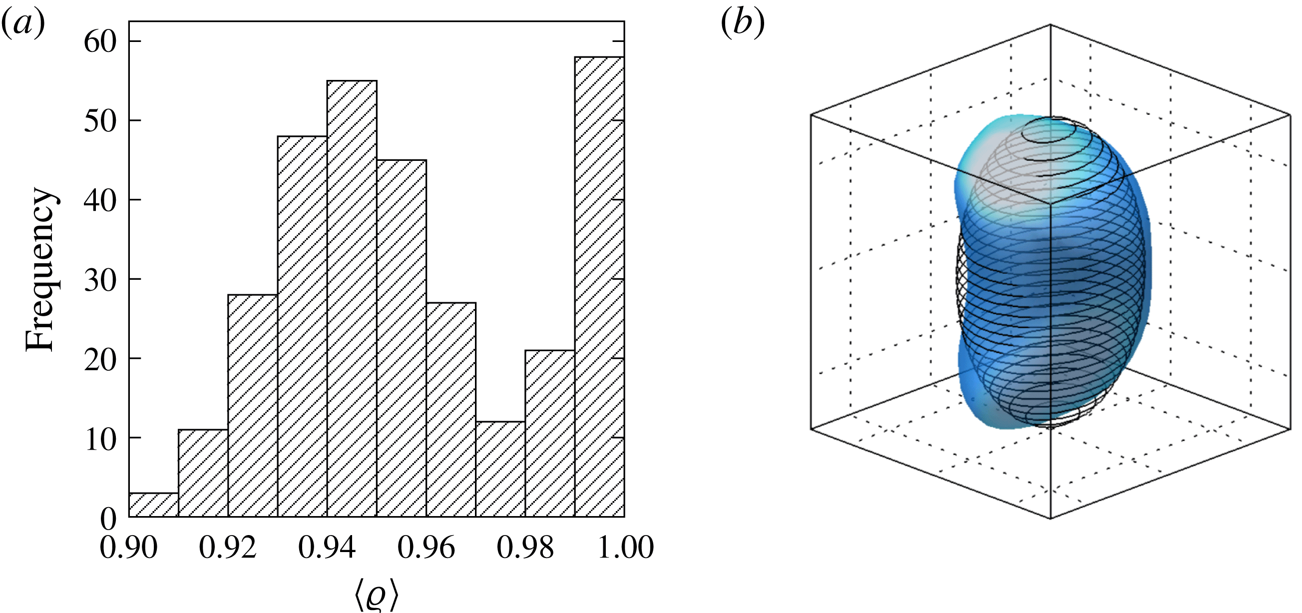
indicating that the vortex is a perfect ellipsoid. Figure 1(a) exhibits a histogram of
 $\langle {\it\varrho}\rangle$
based on all the principal cases studied in this paper (here
 $\langle \cdot \rangle$
denotes a time average over the statistically steady state). Notice that
 $\langle {\it\varrho}\rangle \geqslant 0.9$
for all cases, indicating any departure from the ellipsoidal shape is small. As a result, the semi-axis lengths of the equivalent ellipsoid are good measures of the extent of the vortex along the three corresponding perpendicular directions.
(a) Histogram of the normalised overlap volume
 $\langle {\it\varrho}\rangle$
defined in (3.1). A vortex with a nearly ellipsoidal shape has
 $\langle {\it\varrho}\rangle$
close to unity. The quasi-stable cases contribute to the spike at
 $\langle {\it\varrho}\rangle =1$
. (b) The vortex (smooth surface) and its equivalent oriented ellipsoid (solid lines) for
 $q_{0}=0.25$
,
 ${\it\lambda}_{0}=0.2$
and
 ${\it\mu}_{0}=1.8$
at a late time. The value of
 $\langle {\it\varrho}\rangle =0.9$
for this case is one of the smallest; nevertheless the equivalent ellipsoid manages to capture the aspect ratios and the orientation of the vortex.

It is not always straightforward to define the orientation of a geometrical shape (Žunić, Kopanja & Fieldsend Reference Žunić, Kopanja and Fieldsend2006). Here, however, we find it sufficient to define the orientation of the vortex by that of the equivalent ellipsoid. For the three principal axes of the equivalent ellipsoid, we label the one with the largest projection on the
 $z$
-axis as the vertical axis and denote its semi-length as
 $c(t)$
. The remaining two principal axes are then the horizontal minor axis, of semi-length
 $a(t)$
, and the horizontal major axis, whose semi-length is
 $b(t)$
(but see § 3.1 for special cases when the ellipsoid is tumbling). The orientation of the vortex can be inferred from the tilt angle
 ${\it\theta}(t)$
, defined as the angle between the vertical axis of the equivalent ellipsoid and the
 $z$
-axis. For example, using a case with the smallest
 $\langle {\it\varrho}\rangle$
, figure 1(b) demonstrates that the geometry of the vortex can be effectively captured by the equivalent ellipsoid.
3.1. Evolution and long-term fate
Depending on the initial conditions (
 $q_{0}$
,
 ${\it\lambda}_{0}$
and
 ${\it\mu}_{0}$
), the vortex displays a rich variety of evolutionary behaviours and reaches different equilibrium configurations at large times. We now give an account of the various phenomena observed in the broad range of numerical experiments conducted.
-
(a) Quasi-stable: a quasi-stable vortex deforms extremely slowly and remains close to the initial configuration during the whole simulation. Typically, the fractional change in the semi-axis lengths over
 $100T_{\mathit{ip}}$
is less than 1 %. A quasi-stable vortex often has
${\it\lambda}_{0}\geqslant 0.5$
.
-
(b) Shape alteration: an unstable vortex usually evolves and restablises into a new equilibrium state by changing its shape. We classify the eventual vortex shape as roughly ellipsoidal if
$\langle {\it\varrho}\rangle >0.95$
and non-ellipsoidal if
$\langle {\it\varrho}\rangle \leqslant 0.95$
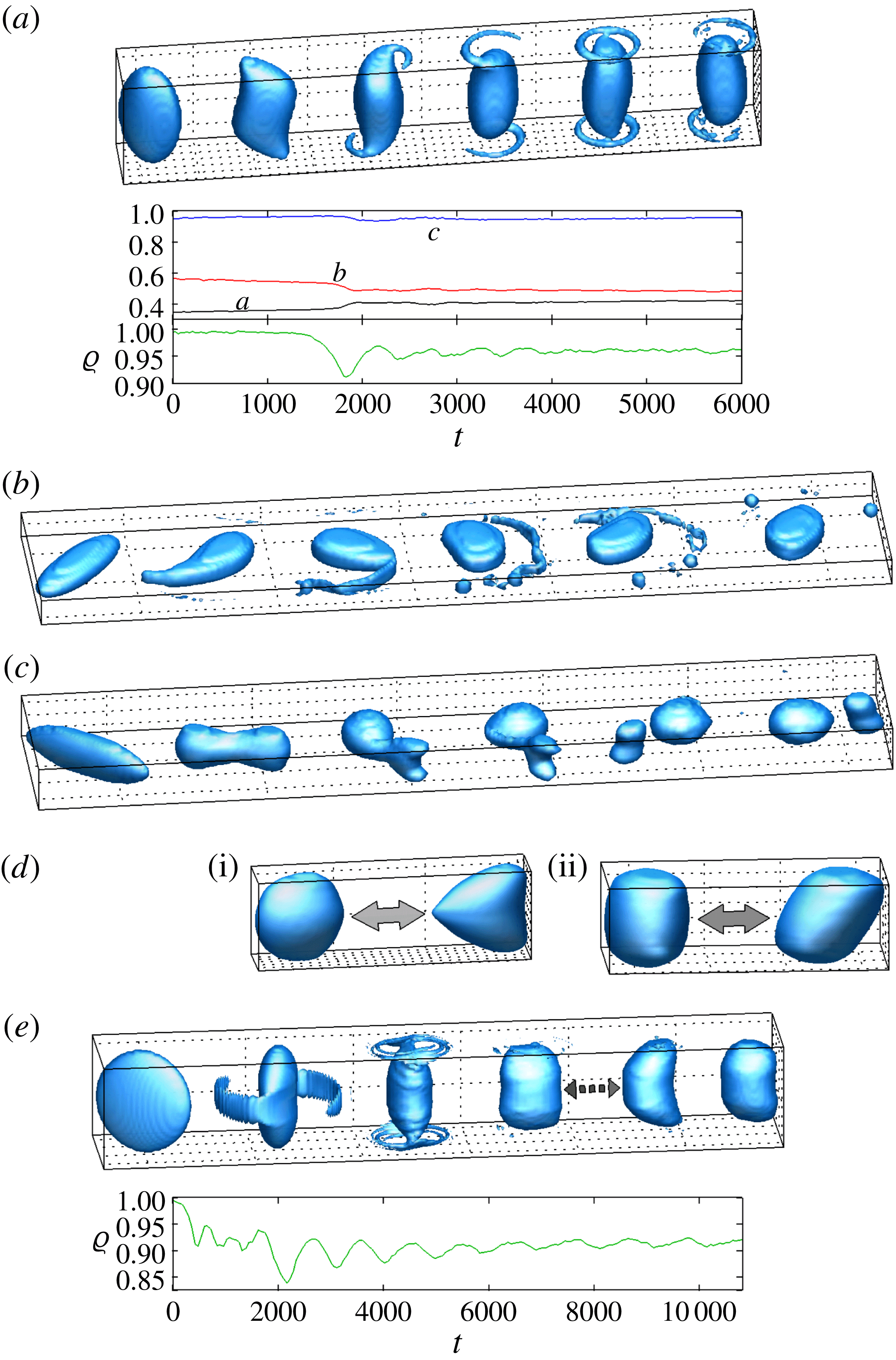
. The evolution process often involves the shedding of vortex filaments (though there are exceptions, see § 3.2). We find that the different scenarios for the nonlinear evolution of a QG vortex described in Dritschel et al. (Reference Dritschel, Scott and Reinaud2005) also apply to our non-hydrostatic Boussinesq system. Figure 2(a) shows an example of filaments being spun off and forming rings near the top and bottom of a prolate vortex (
${\it\mu}_{0}>1$
). -
(c) Binary system: it is not uncommon for ejected filaments to roll up into small satellite vortices which orbit around the main vortex, e.g. see figure 2(b). However, in a few rare cases involving a strongly horizontally elongated vortex, the vortex develops a dumbbell shape before breaking up into a roughly ellipsoidal primary vortex and a smaller secondary vortex. The two vortices revolve around each other forming a binary system. Figure 2(c) shows an example of an anticyclonic binary system. In the analysis presented below, we focus on the primary vortex only. The formation of a binary system has not been observed in QG dynamics.
-
(d) Shape oscillation: as a vortex becomes unstable, instead of converging towards an equilibrium shape, its boundary may start to morph away from and then back to its initial shape periodically. There are also cases where the vortex evolves away from its initial shape and oscillates between two new shapes. Furthermore, it is possible for a vortex to exhibit transient damped shape oscillations as it evolves towards an equilibrium configuration. Two modes of shape oscillation have been observed; they are illustrated in figure 2(d). Figure 2(e) shows a vortex undergoing transient shape oscillation.
-
(e) Tumbling: we find that in some cases where
${\it\mu}_{0}$
is close to unity, the vortex starts to tumble, irrespective of any subsequent development in the vortex shape. The notion of a vertical axis, and hence the definition of the semi-axis lengths, becomes ambiguous for a tumbling ellipsoid. In such cases, after the vortex has reached a statistical steady state, we define
$a(t)$
,
$b(t)$
and
$c(t)$
such that they have the same order in length as
$a_{0}$
,
$b_{0}$
and
$c_{0}$
.


Examples of vortex evolution at different initial horizontal (
 ${\it\lambda}_{0}$
) and vertical (
 ${\it\mu}_{0}$
) aspect ratios. (a) A prolate vortex (
 $q_{0}=0.5$
,
 ${\it\lambda}_{0}=0.6$
,
 ${\it\mu}_{0}=2.4$
) becomes unstable at
 $t\approx 1500$
, spinning off filaments that form rings near the top and bottom of the vortex. Time series of the semi-axis lengths
 $a$
and
 $b$
of its equivalent oriented ellipsoid shows that at the time it becomes unstable, the vortex acquires a near-circular cross-section (
 $\langle {\it\lambda}\rangle =0.87$
). The final equilibrium shape is roughly ellipsoidal as
 ${\it\varrho}>0.95$
at large
 $t$
.(b) PV fragments come off one end of a long oblate vortex (
 $q_{0}=0.5$
,
 ${\it\lambda}_{0}=0.3$
,
 ${\it\mu}_{0}=0.4$
) as it rotates. Two major fragments form satellite vortices orbiting around the main vortex while the finer ones are extended into thin filaments. (c) A binary system formed from a highly horizontally elongated vortex (
 $q_{0}=-0.25$
,
 ${\it\lambda}_{0}=0.2$
,
 ${\it\mu}_{0}=0.6$
). (d) Two modes of vortex shape oscillation: top and bottom of the vortex moving (i) in phase (
 $q_{0}=0.25$
,
 ${\it\lambda}_{0}=0.5$
,
 ${\it\mu}_{0}=1.4$
) or (ii) out of phase (
 $q_{0}=-0.5$
,
 ${\it\lambda}_{0}=0.3$
,
 ${\it\mu}_{0}=1.0$
). (e) A vortex (
 $q_{0}=0.25$
,
 ${\it\lambda}_{0}=0.6$
,
 ${\it\mu}_{0}=2.4$
) oscillates between two different shapes after initial strong filament shedding. The oscillation fades over time as the vortex tends to an equilibrium non-ellipsoidal shape (
 $\langle {\it\varrho}\rangle \approx 0.91$
). This is reflected in the damped oscillation of
 ${\it\varrho}(t)$
starting at
 $t\approx 1800$
.

Phase diagrams showing the equilibrium configuration of a vortex at large time, for varying aspect ratios
 ${\it\lambda}_{0}$
and
 ${\it\mu}_{0}$
and for different PV anomalies or Rossby numbers
 $q_{0}$
: (a) QG; (b)
 $q_{0}=0.25$
; (c)
 $q_{0}=-0.25$
; (d)
 $q_{0}=0.5$
; (e)
 $q_{0}=-0.5$
. The symbols denote the shape of the vortex, as follows: ○, little change from the initial shape at
 $t=0$
; ♢, roughly ellipsoidal (
 $\langle {\it\varrho}\rangle >0.95$
); ▵, non-ellipsoidal (
 $\langle {\it\varrho}\rangle \leqslant 0.95$
);

 $q_{0}=-0.5$
, inside the lower right region bounded by the dashed line are cases in which the vortex deforms smoothly without filament shedding.

3.2. Stability and phase diagram
In § 3.1 above, we described a rich variety of possible behaviours of a vortex and illustrated them in a few examples. We now present results from our full principal data set consisting of 308 simulations. We consider four different values of Rossby number:
 $q_{0}=\pm 0.25$
and
 $\pm 0.5$
. For the aspect ratios,
 ${\it\lambda}_{0}$
varies from 0.2 to 0.8 in steps of 0.1 and
 ${\it\mu}_{0}$
from 0.4 to 2.4 in steps of 0.2. Figure 3(b)–(e) summarises the equilibrium configuration for all cases. For completeness, we also performed simulations of the QG system (Dritschel et al.
Reference Dritschel, Scott and Reinaud2005) representing the limit of zero Rossby number. The results are shown in figure 3(a).
We first investigate the relation between the stability and the geometry of the vortex. Figure 3 shows that, generally, a small vertical aspect ratio and a near-circular horizontal cross-section are favourable conditions for stability. In figure 3, the circles occupy a region in the lower right of the
 ${\it\lambda}_{0}{-}{\it\mu}_{0}$
phase plane. Because the circles indicate that the vortex maintains or oscillates about its initial shape, and in anticipation of the results in § 3.3 below, we loosely refer to this region as the ‘stability region’. As we move away from the stability region by decreasing
 ${\it\lambda}_{0}$
or increasing
 ${\it\mu}_{0}$
, we first encounter cases of unstable vortices which evolve into a roughly ellipsoidal equilibrium shape. This is then followed by the non-ellipsoidal cases as we move further from the stability region. This pattern is especially conspicuous for the QG system. For
 $q_{0}=-0.5$
, no stability region is found within the parameter ranges considered. However, in the region below the dashed line in figure 3(e), the vortex deforms noticeably over several hundred inertial periods in a smooth manner, without shedding filaments. Thus, the evolution in these cases is not unlike that of a quasi-stable vortex except that it happens over a much shorter time scale.
We now turn to the effects of the Rossby number
 $q_{0}$
on the stability of the vortex. From figure 3, we see that as
 $q_{0}$
decreases, the stability region diminishes while its boundary shifts downwards and towards the right. Therefore we conclude that, for fixed aspect ratios
 ${\it\lambda}_{0}$
and
 ${\it\mu}_{0}$
, increasing
 $q_{0}$
enhances stability. As a consequence, a cyclone (
 $q_{0}>0$
) tends to be more stable than an anticyclone (
 $q_{0}<0$
) of the same shape and
 $|q_{0}|$
.
In most cases, the vortex rotates with a fixed orientation about the vertical axis (the vortex may be tilted). However, the orientation of the vortex varies if it is tumbling or undergoing the out-of-phase-type shape oscillation depicted in figure 2(d). An interesting observation from our simulations is that a vortex with a vertical aspect ratio
 ${\it\mu}_{0}$
around unity is most susceptible to orientation variation (hatched symbols in figure 3).
3.3. Aspect ratios of the late-time equilibria
In § 3.2 above, we have seen that the stability of a vortex depends crucially on its aspect ratios
 ${\it\lambda}$
and
 ${\it\mu}$
. In the present section, we look into how
 ${\it\lambda}$
and
 ${\it\mu}$
change as an unstable vortex evolves into an equilibrium configuration. The discussion surrounding (3.1) points out that the equivalent oriented ellipsoid effectively captures the vortex shape. Hence, we can reliably estimate the aspect ratios
 ${\it\lambda}(t)$
and
 ${\it\mu}(t)$
of the vortex at time
 $t$
from
 $a(t)$
,
 $b(t)$
and
 $c(t)$
using expressions analogous to (2.19). The aspect ratios of the equilibrium vortex shape are then represented by the time-averaged values
 $\langle {\it\lambda}\rangle$
and
 $\langle {\it\mu}\rangle$
over the statistically steady state.
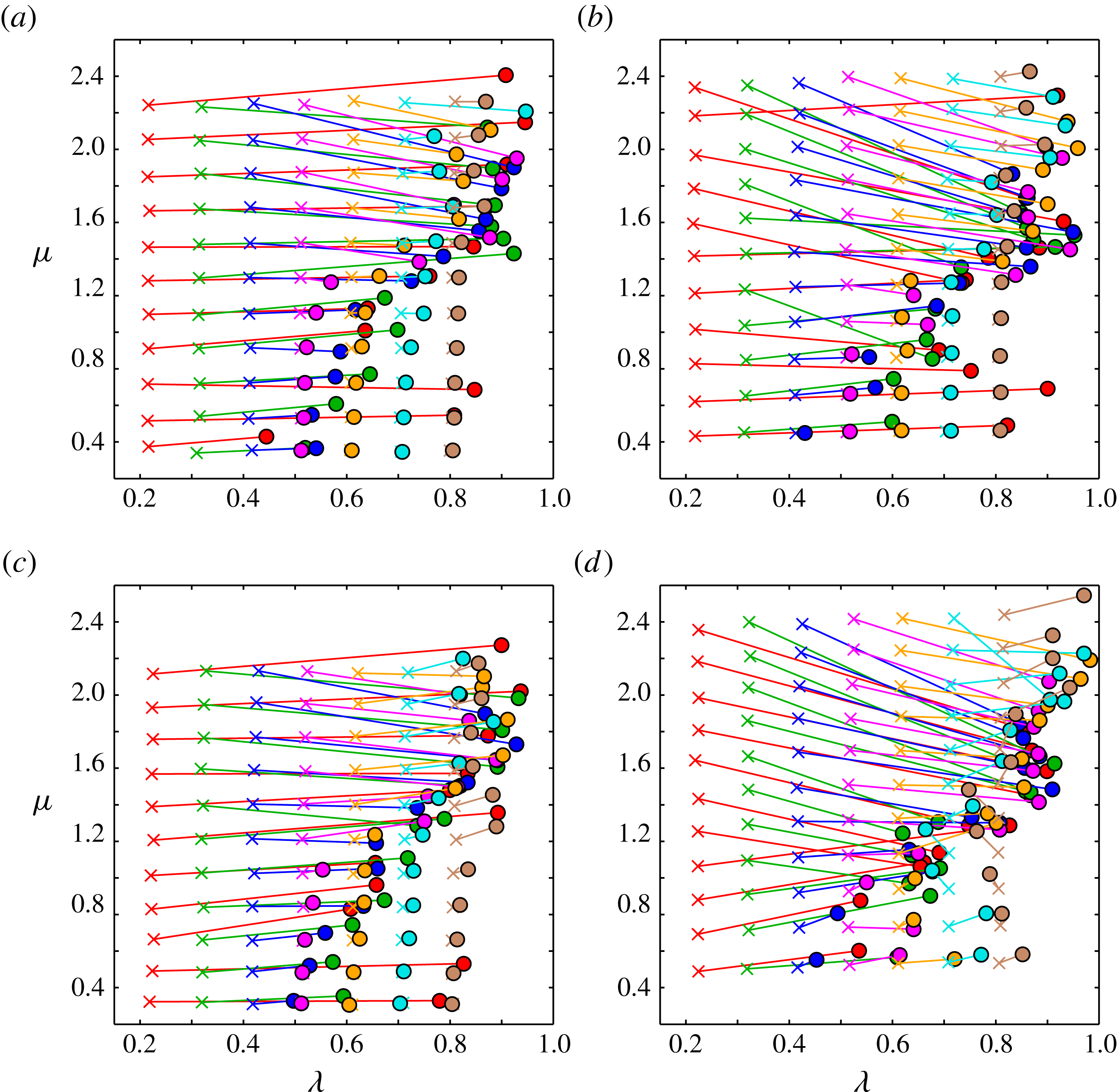
Figure 4 illustrates the change in
 ${\it\lambda}$
and
 ${\it\mu}$
between the initial shape at
 $t=0$
and the equilibrium shape at large
 $t$
. Note that
 $\{{\it\lambda}_{0},{\it\mu}_{0}\}\equiv \{{\it\lambda}(-T_{\mathit{init}}),{\it\mu}(-T_{\mathit{init}})\}$
and there is a small difference between
 $\{{\it\lambda}(0),{\it\mu}(0)\}$
and
 $\{{\it\lambda}_{0},{\it\mu}_{0}\}$
because the vortex is allowed to evolve during the initialisation period. A prominent feature of figure 4 is that
 ${\it\lambda}$
and
 ${\it\mu}$
migrate towards and cluster around the stability boundary (except for the binary systems which evolve deep into the stability region, see § 3.2 for a definition of the ‘stability region’). The deformation of cyclones is mostly achieved with only a minor change in
 ${\it\mu}$
, while a few of the anticyclones show relatively large changes in
 ${\it\mu}$
. In the majority of cases, the vortex eventually acquires a near-circular horizontal cross-section with
 $\langle {\it\lambda}\rangle >0.8$
. The time series in figure 2(a) shows an example of
 $a$
and
 $b$
approaching each other.
Changes in the horizontal aspect ratio
 ${\it\lambda}$
and the vertical aspect ratio
 ${\it\mu}$
of the vortex. Crosses are values at the end of the initialisation period
 $t=0$
. Solid circles are time-averaged values
 $\langle {\it\lambda}\rangle$
and
 $\langle {\it\mu}\rangle$
over the statistically steady state at large time. (a)
 $q_{0}=0.25$
; (b)
 $q_{0}=-0.25$
; (c)
 $q_{0}=0.5$
; (d)
 $q_{0}=-0.5$
.

We emphasise that, with the exception of the quasi-stable cases, the final equilibrium shape of the vortex is not a perfect ellipsoid, see figure 1. Thus, the clustering of
 $\langle {\it\lambda}\rangle$
and
 $\langle {\it\mu}\rangle$
seen in figure 4 suggests that the stability of the vortex depends primarily on the aspect ratios – gross measures of the vortex shape – not on the detailed vortex shape. The pattern displayed in figure 4 has interesting implications for the vortex rotation rate, as elaborated in § 4.
3.4. Discussion
In naturally occurring geophysical flows, the process of vortex formation is likely to be highly varied and complex. Therefore, one may expect to observe vortices with a wide range of shapes. However, observed ocean eddies generally appear to have roughly circular horizontal cross-sections. This has motivated much previous work on vortex stability in various idealised systems and has led to the idea that vortices which are highly elongated at birth are unstable and quickly evolve into more stable configurations; see for example Cushman-Roisin (Reference Cushman-Roisin1986) and Carton (Reference Carton2001) and references therein.
For the ellipsoidal vortices studied in the present work, we find that, in the vast majority of cases, instability results in a transition to another roughly ellipsoidal vortex, always with a more circular horizontal cross-section and often with a scaled vertical aspect ratio
 ${\it\mu}$
closer to unity (see figure 4). A key result of the present investigation is the identification of these quasi-stable vortex structures emerging as the end states of evolution starting from a wide range of initial shapes, i.e. the identification of the ‘stability region’ mapped out by the circles in figure 4.
The form of the stability region constrains the possible geometry of a stable vortex. This leads to some interesting consequences. As just remarked, all unstable vortices restabilise by increasing their horizontal aspect ratio
 ${\it\lambda}$
toward unity. At equilibrium, we find
 ${\it\lambda}\gtrsim 0.5$
. Furthermore, the most probable value for
 ${\it\lambda}$
is around 0.8. This echoes what has been reported in many observations of ocean eddies (Paillet et al.
Reference Paillet, Le Cann, Carton, Morel and Serpette2002; Lentini et al.
Reference Lentini, Goni and Olson2006; Kim Reference Kim2010; Park, Woo & Ryu Reference Park, Woo and Ryu2012). Also, tall vortices (large
 ${\it\mu}$
) are restricted to have
 ${\it\lambda}\approx 1$
while flat vortices (small
 ${\it\mu}$
) can exhibit a wider range of
 ${\it\lambda}$
. Finally, since the stability boundary migrates towards smaller
 ${\it\lambda}$
as
 $q_{0}$
increases, stable highly eccentric vortices (with small
 ${\it\lambda}$
) are most likely to be strongly ageostrophic cyclones (with
 $q_{0}$
near unity). On the other hand, strongly ageostrophic anticyclones are restricted to have nearly circular horizontal cross-section. In the light of the present results, it would be worthwhile to examine observational data to see where ocean eddies lie in figure 4.
As regards ageostrophic effects on stability (in the sense explained in § 3.1), we find robustly that vortices are increasingly stable (over a broader range of initial shapes) as the signed Rossby number
 $q_{0}$
increases. While our analysis has largely been restricted to the range
 $-0.5\leqslant q_{0}\leqslant 0.5$
, a few additional simulations at
 $q_{0}=0.75$
suggest that this trend applies over a wider range of
 $q_{0}$
. We cannot examine
 $|q_{0}|\gtrsim 1$
with the PV-conserving numerical algorithm employed here because then we cannot invert the PV (Dritschel & Viúdez Reference Dritschel and Viúdez2003).
4. Vortex rotation rate
In the majority of cases considered here, the vortex shape, specifically the boundary of the region of non-zero PV anomaly, rotates about the vertical axis at an approximately constant angular velocity
 ${\it\Omega}$
after the system has reached a statistically steady state. In the exceptional cases when the vortex shape oscillates or the vortex is tumbling, the magnitude or the direction of the angular velocity, or both, vary with time. For all cases, we compute the vortex rotation rate
 ${\it\Omega}(t)$
by tracking the projection of the horizontal major axis (defined in § 3) of the equivalent ellipsoid on the
 $x{-}y$
plane. Figure 5 shows
 ${\it\Omega}(t)$
for a few selected cases, illustrating a sample of the varied behaviours that are possible. Here, we examine the late-time average rotation rate
 $\langle {\it\Omega}\rangle$
of the equilibrium state, in particular its dependence on
 $\langle {\it\lambda}\rangle$
and
 $\langle {\it\mu}\rangle$
and its deviation from the rotation rate
 ${\it\Omega}_{\mathit{QG}}$
of a QG ellipsoid (Meacham Reference Meacham1992; Dritschel et al.
Reference Dritschel, Scott and Reinaud2005):
 $$\begin{eqnarray}{\it\Omega}_{\mathit{QG}}({\it\lambda},{\it\mu})=(q_{0}\,f)\,{\it\mu}\,\frac{{\it\lambda}^{-1}\,R_{D}({\it\mu}^{2},{\it\lambda},{\it\lambda}^{-1})-{\it\lambda}\,R_{D}({\it\mu}^{2},{\it\lambda}^{-1},{\it\lambda})}{3({\it\lambda}^{-1}-{\it\lambda})},\end{eqnarray}$$
where
 $$\begin{eqnarray}R_{D}(x,y,z)=\frac{3}{2}\int _{0}^{\infty }\frac{\text{d}t}{\sqrt{(t+x)(t+y)(t+z)^{3}}}\end{eqnarray}$$
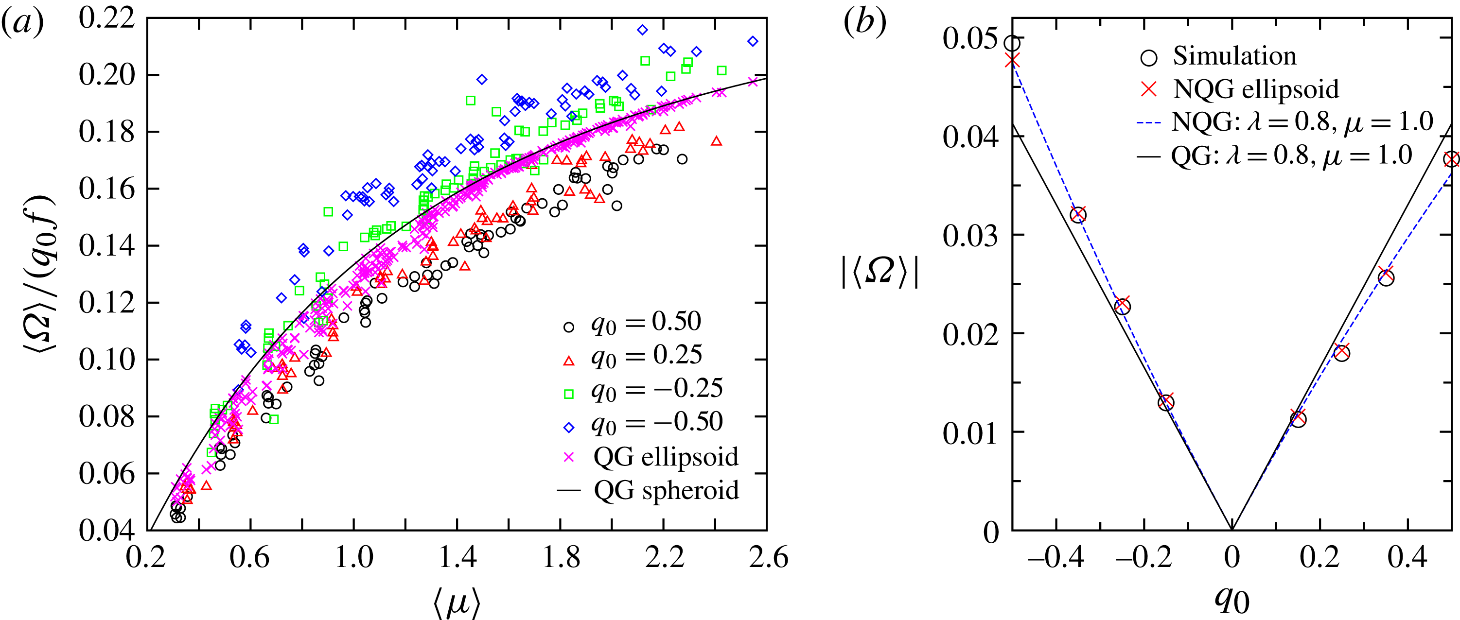
is Carlson’s symmetric elliptic integral of the second kind (Carlson & Gustafson Reference Carlson and Gustafson1994). Our main findings are summarised in figure 6(a), presenting a scatter plot of
 $\langle {\it\Omega}\rangle$
versus
 $\langle {\it\mu}\rangle$
for all cases in the principal data set. The corresponding QG ellipsoid rotation rate for each case, i.e.
 ${\it\Omega}_{\mathit{QG}}(\langle {\it\lambda}\rangle ,\langle {\it\mu}\rangle )$
, is also included in the plot.
Rotation rate
 ${\it\Omega}(t)$
for a vortex which (a) rotates approximately steadily at late times (
 $\langle {\it\lambda}\rangle =0.90$
and
 $\langle {\it\mu}\rangle =2.27$
for this case); (b) exhibits shape oscillations as shown in figure 2(d) (the period is
 ${\approx}150T_{\mathit{ip}}$
; note
 ${\it\Omega}(t)$
decreases in the phase of the oscillation when the vortex is extending horizontally); (c) starts to tumble after a period of steady rotation; the vortex maintains its initial ellipsoidal shape throughout the simulation. The initial configurations are: (a)
 $q_{0}=0.5,{\it\lambda}_{0}=0.2,{\it\mu}_{0}=2.4$
; (b)
 $q_{0}=0.25,{\it\lambda}_{0}=0.5,{\it\mu}_{0}=1.4$
; (c)
 $q_{0}=-0.25,{\it\lambda}_{0}=0.7,{\it\mu}_{0}=1.0$
.

(a) Scatter plot showing the correlation between the rotation rate
 $\langle {\it\Omega}\rangle$
(normalised by
 $q_{0}\,f$
) and the vertical aspect ratio
 $\langle {\it\mu}\rangle$
when the vortex is in approximate equilibrium at large time. For each simulation, we also calculate the corresponding QG ellipsoid rotation rate
 ${\it\Omega}_{\mathit{QG}}(\langle {\it\lambda}\rangle ,\langle {\it\mu}\rangle )$
using (4.1) (its normalised values are plotted as crosses). For reference, the rotation rate of a QG spheroid
 ${\it\Omega}_{\mathit{QG}}({\it\lambda}=1,{\it\mu})$
is included as a solid line. (b)
 $|\langle {\it\Omega}\rangle |$
versus
 $q_{0}$
for selected simulations having similar aspect ratios (circles). At each
 $q_{0}$
, the vortex has
 $\{\langle {\it\lambda}\rangle ,\langle {\it\mu}\rangle \}$
within 10 % of
 $\{0.8,1.0\}$
. The rotation rate of an NQG ellipsoid (see text) with the same aspect ratios
 $\{\langle {\it\lambda}\rangle ,\langle {\it\mu}\rangle \}$
is plotted by a cross for each
 $q_{0}$
. The dashed and solid lines give, respectively, the rotation rate of an NQG ellipsoid and a QG ellipsoid, both having aspect ratios
 $\{{\it\lambda},{\it\mu}\}=\{0.8,1.0\}$
. Only the QG rotation rate is symmetric about
 $q_{0}=0$
.

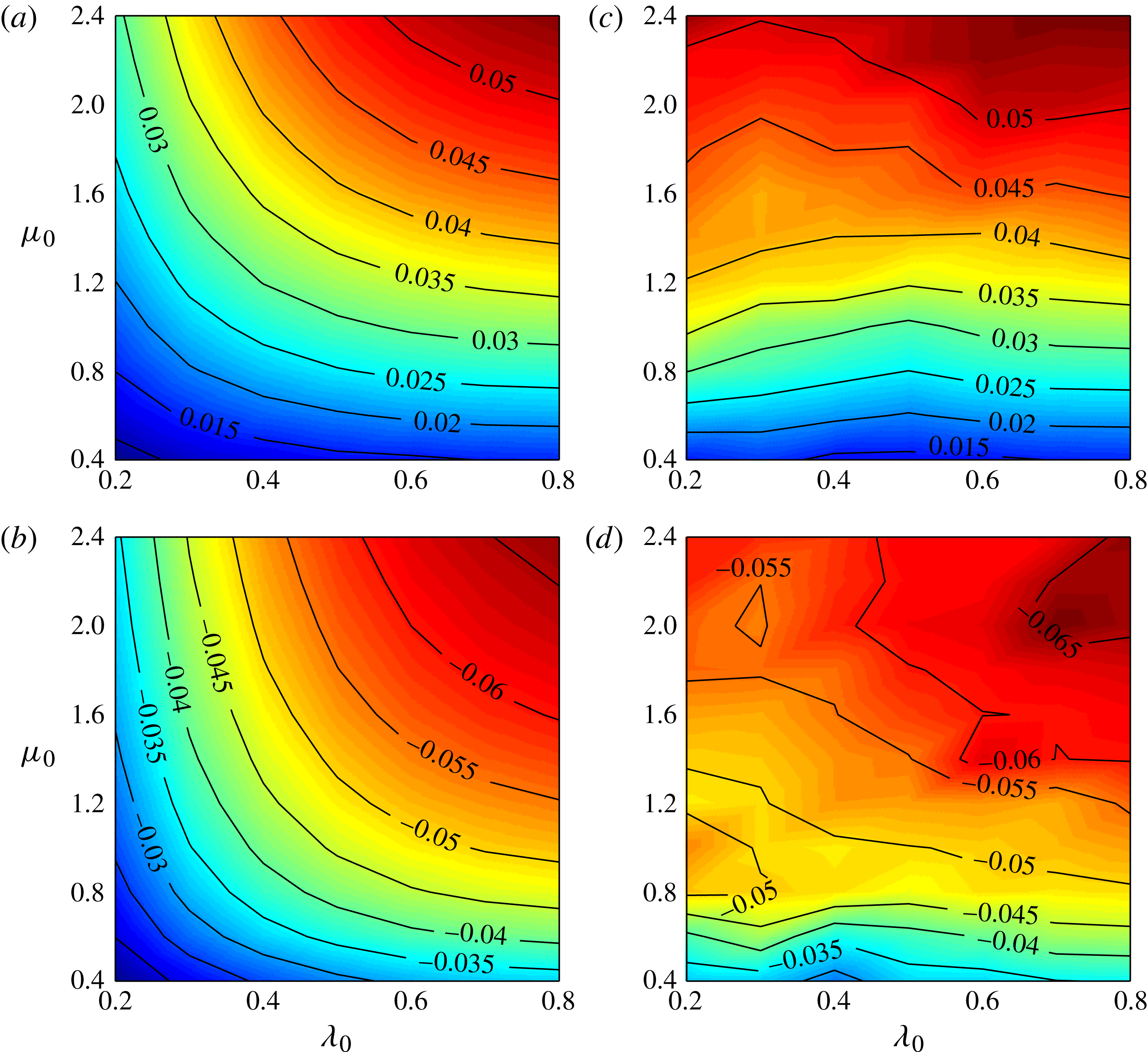
A remarkable feature of figure 6(a) is that the data for each
 $q_{0}$
strongly cluster around a single curve, implying that
 $\langle {\it\lambda}\rangle$
plays only a minimal role here. On the other hand,
 $\langle {\it\Omega}\rangle$
shows a strong dependence on
 $\langle {\it\mu}\rangle$
. This is a consequence of the evolutionary changes exhibited by
 $\langle {\it\lambda}\rangle$
and
 $\langle {\it\mu}\rangle$
in figure 4. To elucidate, we plot
 ${\it\Omega}_{0}\equiv {\it\Omega}(t=0)$
and
 $\langle {\it\Omega}\rangle$
as a function of the initial aspect ratios
 ${\it\lambda}_{0}$
and
 ${\it\mu}_{0}$
in figure 7 (see appendix B for the method to compute
 ${\it\Omega}_{0}$
). For a quasi-stable vortex,
 $\langle {\it\Omega}\rangle \approx {\it\Omega}_{0}$
,
 $\langle {\it\lambda}\rangle \approx {\it\lambda}_{0}$
and
 $\langle {\it\mu}\rangle \approx {\it\mu}_{0}$
since the initial ellipsoidal shape is maintained. For an unstable vortex, figures 4 and 7 together suggest that at late times,
 $\langle {\it\Omega}\rangle$
is close to the rotation rate of a quasi-stable ellipsoid with the same
 $\langle {\it\lambda}\rangle$
and
 $\langle {\it\mu}\rangle$
. In other words, for a vortex whose aspect ratios evolve from
 $\{{\it\lambda}_{0},{\it\mu}_{0}\}$
to
 $\{\langle {\it\lambda}\rangle ,\langle {\it\mu}\rangle \}$
, the late-time average rotation rate
 $\langle {\it\Omega}\rangle$
is estimated well by
 ${\it\Omega}_{0}({\it\lambda}_{0}=\langle {\it\lambda}\rangle ,{\it\mu}_{0}=\langle {\it\mu}\rangle )$
. This can be seen by comparing figures 7(a) with 7(c) and 7(b) with 7(d) (see also figure 5
a for an example). The fact that
 $\{\langle {\it\lambda}\rangle ,\langle {\it\mu}\rangle \}$
mostly clusters around the stability boundary, together with the observation that
 ${\it\Omega}_{0}$
depends weakly on
 ${\it\lambda}_{0}$
for
 $0.5\leqslant {\it\lambda}_{0}\leqslant 1$
, imply that
 $\langle {\it\lambda}\rangle$
is not important in determining
 $\langle {\it\Omega}\rangle$
. It also follows that the
 $\langle {\it\mu}\rangle$
-dependence of
 $\langle {\it\Omega}\rangle$
seen in figure 6(a) is well approximated by
 ${\it\Omega}_{0}({\it\lambda}_{0},{\it\mu}_{0}=\langle {\it\mu}\rangle )$
for some fixed
 ${\it\lambda}_{0}\approx 1$
.
The initial rotation rate
 ${\it\Omega}_{0}$
at time
 $t=0$
and the average rotation rate
 $\langle {\it\Omega}\rangle$
of the equilibrium state at large
 $t$
as a function of the initial aspect ratios
 ${\it\lambda}_{0}$
and
 ${\it\mu}_{0}$
: (a)
 ${\it\Omega}_{0}$
for
 $q_{0}=0.5$
, (b)
 ${\it\Omega}_{0}$
for
 $q_{0}=-0.5$
, (c)
 $\langle {\it\Omega}\rangle$
for
 $q_{0}=0.5$
, (d)
 $\langle {\it\Omega}\rangle$
for
 $q_{0}=-0.5$
. For a quasi-stable vortex,
 $\langle {\it\Omega}\rangle \approx {\it\Omega}_{0}$
. Assuming
 $\langle {\it\Omega}\rangle$
depends mainly on
 $\langle {\it\lambda}\rangle$
and
 $\langle {\it\mu}\rangle$
but not on the exact vortex shape (at least when
 $\langle {\it\varrho}\rangle \approx 1$
), then
 $\langle {\it\Omega}\rangle$
for an unstable vortex should be close to the rotation rate of a quasi-stable ellipsoid with the same
 $\langle {\it\lambda}\rangle$
and
 $\langle {\it\mu}\rangle$
. Hence, pictorially speaking,
 $\langle {\it\Omega}\rangle$
in (c) and (d) is obtained by flattening out the contours of
 ${\it\Omega}_{0}$
in (a) and (b). For
 $q_{0}=0.5$
, the weak dependence of
 $\langle {\it\Omega}\rangle$
on
 ${\it\lambda}_{0}$
reflects the fact that
 $\langle {\it\mu}\rangle \approx {\it\mu}_{0}$
, as evident in figure 4. For
 $q_{0}=-0.5$
, the small irregularities in
 $\langle {\it\Omega}\rangle$
around
 $(0.2,1.0)$
and
 $(0.3,2.0)$
are caused by the significant variation in the vertical aspect ratio
 ${\it\mu}$
in these regions, as seen from figure 4. Cases with
 $q_{0}=\pm 0.25$
show similar behaviour.

Figure 6(a) also reveals that ageostrophic effects occurring at finite Rossby number result in a visible asymmetry between cyclones and anticyclones: for the same aspect ratios
 $\langle {\it\lambda}\rangle$
and
 $\langle {\it\mu}\rangle$
and PV anomaly
 $|q_{0}|$
, an anticyclone rotates faster than a cyclone. The corresponding
 $|{\it\Omega}_{\mathit{QG}}|$
denoted by crosses in figure 6(a) lies somewhere between the cyclonic and the anticyclonic rotation rates. Cyclone–anticyclone asymmetry can be traced back to the nonlinear terms in (2.16) which break the invariance of the PV inversion under the transformation
 $(q,{\bf\varphi})\rightarrow -(q,{\bf\varphi})$
. Moreover this asymmetry can be quantitatively captured by a next-order correction to QG theory, as shown next.
4.1. Vortex rotation rate estimated by a higher-order balanced model
A number of balanced models have been developed to extend the QG approximation (see e.g. Warn et al.
Reference Warn, Bokhove, Shepherd and Vallis1995, Muraki, Snyder & Rotunno Reference Muraki, Snyder and Rotunno1999 and references therein). Here, we adopt the nonlinear quasi-geostrophic (NQG) balanced model of McKiver & Dritschel (Reference McKiver and Dritschel2008), see appendix C. The NQG balanced model uses a Rossby-number expansion to second order,
 $O(q_{0}^{2})$
, except that it retains the exact definition of PV. This greatly improves the estimate of the underlying balanced flow, as demonstrated explicitly in McKiver & Dritschel (Reference McKiver and Dritschel2008). The resulting nonlinear PV inversion relations allow one to reconstruct the velocity and buoyancy fields to
 $O(q_{0}^{2})$
from a given instantaneous PV field.
In figure 6(b), we plot
 $|\langle {\it\Omega}\rangle |$
versus
 $q_{0}$
for several cases having similar aspect ratios
 $\langle {\it\lambda}\rangle$
and
 $\langle {\it\mu}\rangle$
. Corresponding to each of these cases, we construct the velocity field from an ellipsoid of uniform PV with the same
 $\langle {\it\lambda}\rangle$
,
 $\langle {\it\mu}\rangle$
and
 $q_{0}$
by NQG PV inversion. The rotation rates of such NQG-balanced ellipsoids are then calculated (see appendix B). We find close agreement, typically within 3 %, between the theoretical NQG rotation rate and the data across all
 $q_{0}$
. Figure 6(b) also shows the rotation rate of an NQG ellipsoid with
 ${\it\lambda}=0.8$
and
 ${\it\mu}=1.0$
as a function of
 $q_{0}$
. These results clearly reveal the emergence of asymmetry in the cyclonic and anticyclonic rotation rate as soon as finite Rossby number effects are taken into account.
4.2. Discussion
We have seen above that
 ${\it\Omega}$
has a strong dependence on the vertical aspect ratio
 ${\it\mu}$
. Moreover, ageostrophic effects at
 $O(q_{0}^{2})$
make anticyclones spin faster than cyclones, particularly at large
 ${\it\mu}$
(see figure 6). In observations, for the cyclonic Gulf Stream cold core ring reported in Spence & Legeckis (Reference Spence and Legeckis1981) (
 ${\it\lambda}=0.65$
,
 ${\it\mu}=1.10$
,
 $q_{0}=0.52$
and
 $f=8.6\times 10^{-5}\,\text{s}^{-1}$
), we estimate
 ${\it\Omega}/{\it\Omega}_{\mathit{QG}}=0.73<1$
; while for the anticyclonic meddy documented by Hebert, Oakey & Ruddick (Reference Hebert, Oakey and Ruddick1990) (
 ${\it\lambda}=0.71$
,
 ${\it\mu}=0.32$
,
 $q_{0}=0.35$
and
 $f=1.0\times 10^{-4}\,\text{s}^{-1}$
), we estimate
 ${\it\Omega}/{\it\Omega}_{\mathit{QG}}=1.03\gtrsim 1$
. These two individual cases appear to support our findings. Exceptionally, the anticyclonic meddy ‘Ulla’ has
 ${\it\Omega}/{\it\Omega}_{\mathit{QG}}<1$
. This is perhaps not surprising as Ulla ‘is not just another meddy’ (Paillet et al.
Reference Paillet, Le Cann, Carton, Morel and Serpette2002) and has some peculiar features. In order to fully verify the
 $O(q_{0}^{2})$
effects discussed here, laboratory experiments under controlled conditions are probably needed. Additionally, there appears to be a wealth of untapped numerical simulation data available from high-resolution ocean models. This should be exploited.
5. Balance
5.1. Definitions and method of analysis
The control exerted by PV on the dynamics of vortices in rotating stably stratified geophysical flows can be, for all practical purpose, nearly complete, with IGWs playing a negligible role. This state of affairs is known as ‘balance’. Balance is favoured when the magnitude of the Rossby number
 $|q_{0}|\lesssim 1$
and the frequency ratio
 $f/N\lesssim 1$
, even in strongly turbulent flows (Dritschel & Viúdez Reference Dritschel and Viúdez2007; Dritschel & McKiver Reference Dritschel and McKiver2014), at least for carefully prepared initial conditions.
As described in § 2.4, we initialise each flow by artificially ramping up the PV anomaly over many inertial periods while otherwise solving the full equations of motion. This results in an ‘initial’ state nearly void of IGWs when
 $|q_{0}|\lesssim 1$
and
 $f/N\lesssim 1$
. To explore the possible spontaneous emission of IGWs at later times and to estimate their contribution to the dynamics, we need to quantify balance and the residual imbalance or IGW activity. One approach to diagnose the balanced component from a given PV field is to invert the ‘balance conditions’ obtained from a Rossby number expansion of the governing equations. Such balance conditions define an instantaneous state of balance. The traditional QG balance and the higher-order NQG balance in § 4.1 fall into this category. Here, we take another approach, called optimal potential vorticity (OPV) balance (Viúdez & Dritschel Reference Viúdez and Dritschel2004), which does not enforce any specific balanced conditions but instead seeks the ‘minimally imbalanced’ state through a numerical iterative procedure.
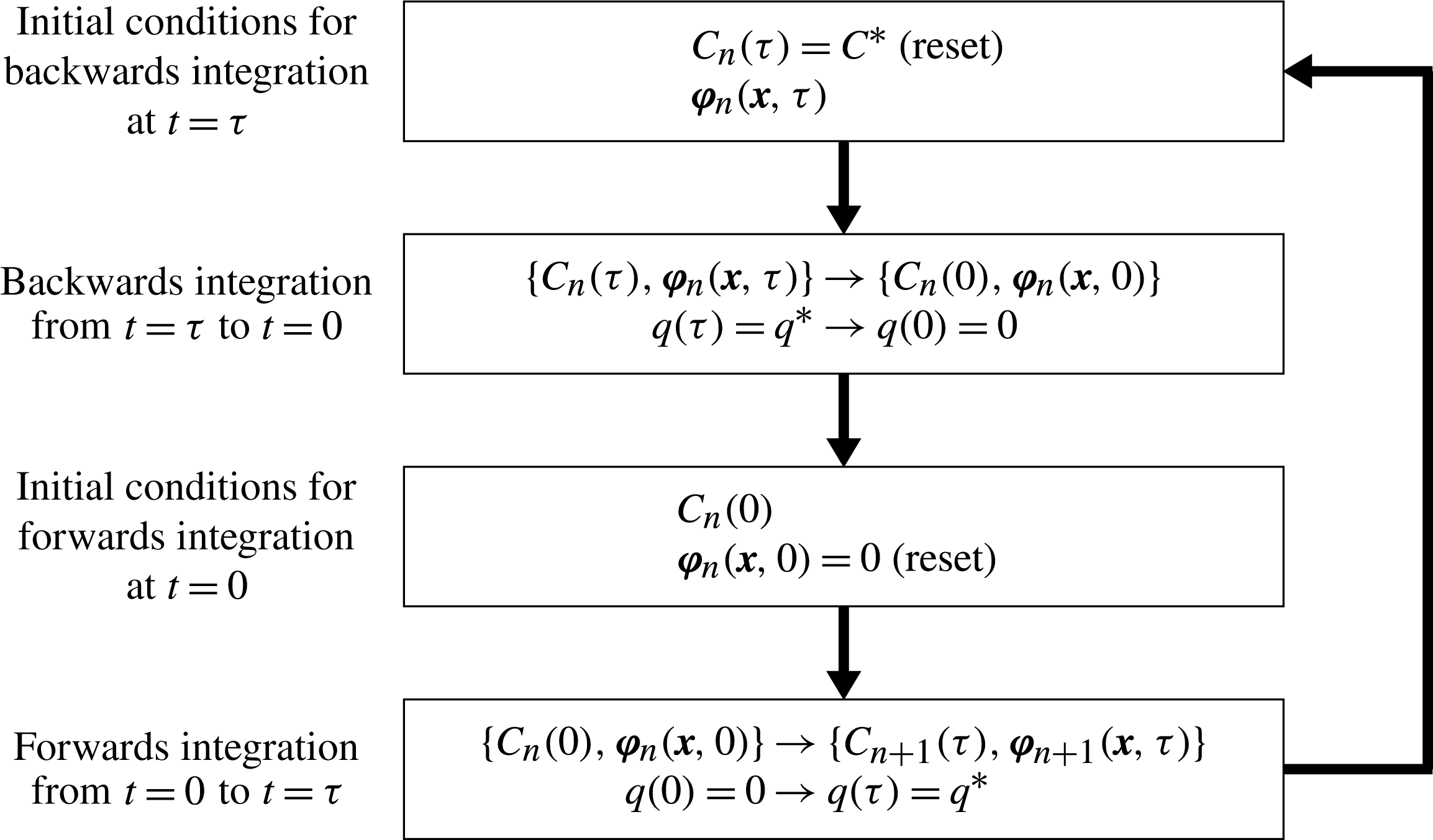
Given the PV distribution at some chosen diagnostic time
 $t$
, the OPV procedure carries out a series of artificial forward and backward integrations of the equations of motion, over a specified time period
 ${\it\tau}$
. Each integration involves ramping up or ramping down the PV anomaly. The objective is to arrive at the original given PV distribution from a different one in a state of rest at time
 $t-{\it\tau}$
, after ramping up the PV anomaly and otherwise solving the full equations of motion. The resulting fields are called ‘balanced’, even though they may contain small residual imbalance (Dritschel & Viúdez Reference Dritschel and Viúdez2007; Viúdez Reference Viúdez2007). Note, the balance depends only on the PV distribution provided and the ramp period
 ${\it\tau}$
. The choice of
 ${\it\tau}$
is strongly affected by the amount of distortion of the PV distribution occurring between
 $t-{\it\tau}$
(the base distribution) and
 $t$
(the given target distribution) during the ramp. If
 ${\it\tau}$
is too long, the base distribution is too distorted to ever converge to the target one. A compromise must be made. Following previous studies (Dritschel & Viúdez Reference Dritschel and Viúdez2007; McKiver & Dritschel Reference McKiver and Dritschel2008) and after conducting further tests here, we took
 ${\it\tau}$
to be four inertial periods. This is sufficiently long not to excite significant IGW activity, though not long enough to avoid all of it. In this sense, it is better to view OPV balance as a procedure which seeks the minimally imbalanced state, subject to the constraint that the base PV distribution can actually evolve into the target PV distribution. The technical details of OPV balance are summarised in appendix D.
Given the OPV balanced flow
 ${\bf\varphi}_{\mathit{bal}}$
at a chosen diagnostic time
 $t$
, the imbalanced flow (or ‘imbalance’) is defined simply by subtraction from the full flow,
 $$\begin{eqnarray}{\bf\varphi}_{\mathit{imb}}={\bf\varphi}-{\bf\varphi}_{\mathit{bal}}.\end{eqnarray}$$
The balanced flow is further divided into a QG balanced part
 ${\bf\varphi}_{\mathit{QG}}=(0,0,{\it\phi}_{\mathit{QG}})$
and the remaining ‘ageostrophic’ balanced part
 $$\begin{eqnarray}{\bf\varphi}_{\mathit{AGb}}={\bf\varphi}_{\mathit{bal}}-{\bf\varphi}_{\mathit{QG}}.\end{eqnarray}$$
Here,
 ${\it\phi}_{\mathit{QG}}$
is defined in the standard way, inverting the QG linear operator on the PV anomaly
 $q$
(see (C 3) in appendix C) on flat isopycnal surfaces, not on the actual displaced surfaces (the displacement is proportional to
 $q_{0}$
, and the effect of this displacement is
 $O(q_{0}^{2})$
on the balanced flow and therefore an ageostrophic effect).
We next focus on two cases which serve to illustrate how the nature of both the balanced flow and the imbalance vary with the vortex shape and the Rossby number
 $q_{0}$
. In each case, we examine a time at or near the end of the simulation when the vortex is in a near-equilibrium state. As discussed below, the imbalance is often largest during a period of instability and rapid change, though it never contributes significantly to the total energy. We finish by examining the fractional energy associated with the balanced and imbalanced flow components as a function of the Rossby number
 $q_{0}$
.
5.2. Oblate weakly eccentric vortices
We first look at an oblate cyclone and anticyclone at
 $|q_{0}|=0.25$
with
 ${\it\lambda}_{0}=0.8$
and
 ${\it\mu}_{0}=0.4$
. These vortices are quasi-stable: in the late-time equilibrium state
 $\langle {\it\lambda}\rangle \approx$
 ${\it\lambda}(t=0)=0.81$
in both cases, and
 $\langle {\it\mu}\rangle \approx {\it\mu}(t=0)=0.35$
and 0.46 for the cyclone and anticyclone respectively.
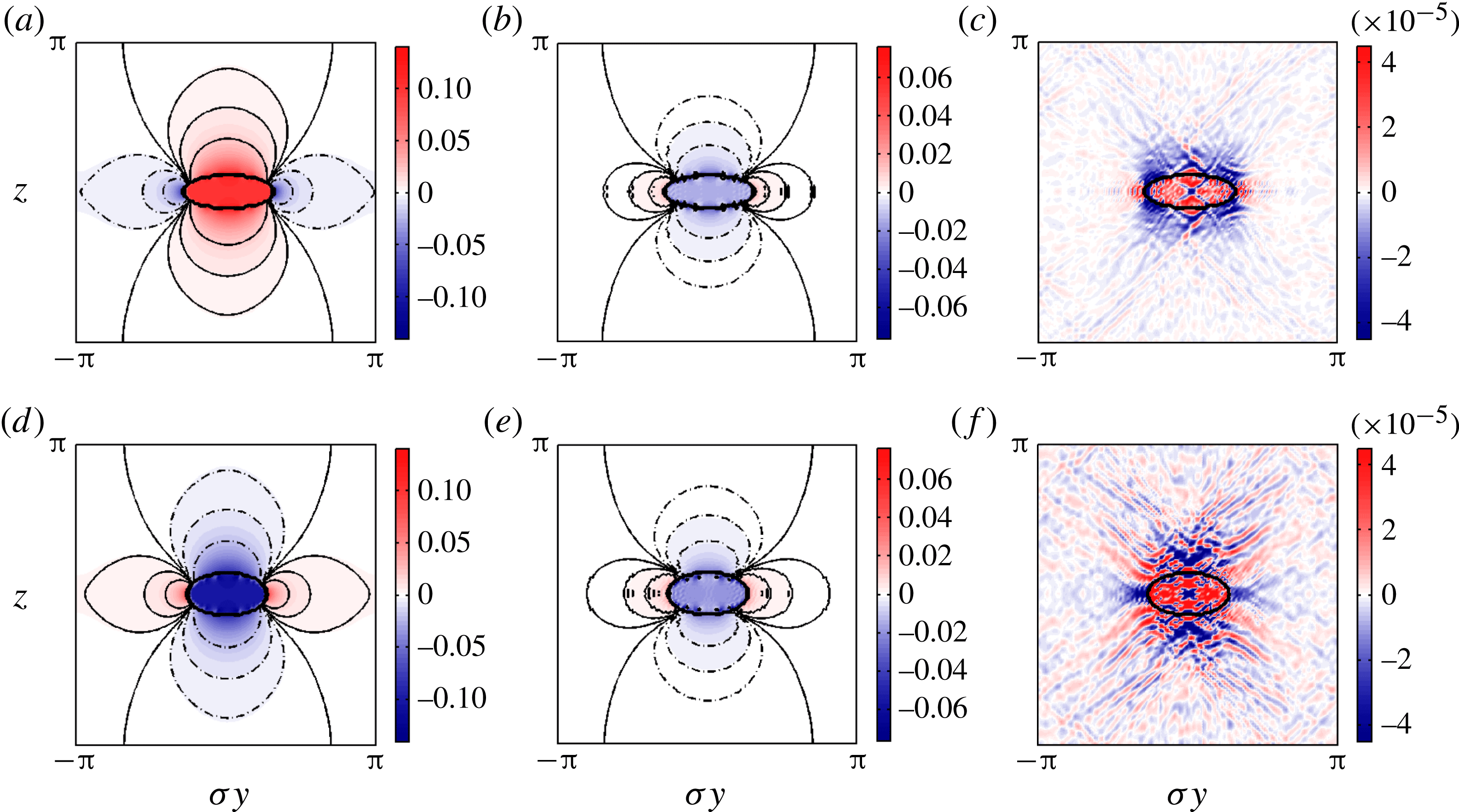
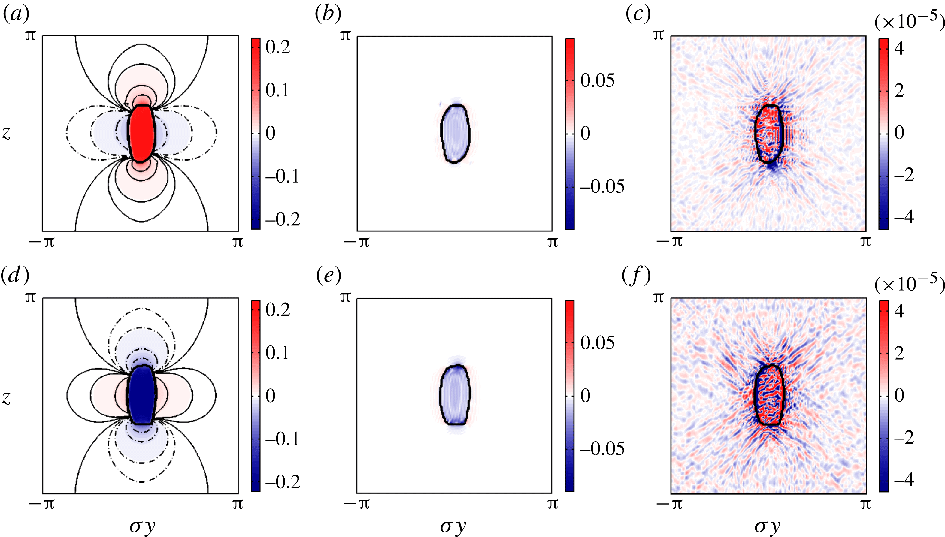
Figure 8(a–c) shows the balanced and imbalanced components of the scaled vertical vorticity
 ${\it\zeta}/f$
for the cyclone while figure 8(d–f) shows the analogous fields for the anticyclone. First of all, the QG balanced fields are entirely as expected: positive vorticity inside the vortex for the cyclone and negative for the anticyclone. Just outside, the vorticity switches sign. Again, this is consistent since, inside the cyclone, vortex lines are more bunched together, while outside they must be more spread out in order to relax to the undisturbed state with absolute vorticity
 $f\hat{\boldsymbol{k}}$
far from the vortex. The anticyclone is exactly the opposite. On the other hand, the ageostrophic balanced fields do not preserve the antisymmetry between cyclones and anticyclones. In both cases,
 ${\it\zeta}_{\mathit{AGb}}$
is negative inside the vortex, and weakly positive just outside of it. This is because
 ${\it\zeta}_{\mathit{AGb}}$
depends quadratically, to leading order, on the QG balanced fields (see appendix C or, explicitly, (2.23) of McKiver & Dritschel (Reference McKiver and Dritschel2008)).
A vertical
 $y{-}z$
cross-section at
 $x=-{\it\sigma}^{-1}{\rm\pi}/32$
of the scaled vertical vorticity
 ${\it\zeta}/f$
for a cyclonic vortex or ‘cyclone’ (a–c) and an anticyclonic vortex or ‘anticyclone’ (d–f) with
 $q_{0}=\pm 0.25$
respectively. The initial aspect ratios are
 ${\it\lambda}_{0}=0.8$
and
 ${\it\mu}_{0}=0.4$
in both cases. The QG balanced part
 ${\it\zeta}_{\mathit{QG}}/f$
is shown in (a) and (d), the ageostrophic balanced part
 ${\it\zeta}_{\mathit{AGb}}/f$
in (b) and (e), the imbalanced part
 ${\it\zeta}_{\mathit{imb}}/f$
in (c) and (f). The fields are depicted at
 $t=480T_{\mathit{ip}}$
. The bold black contour indicates the vortex edge, while the thin solid and thin dashed contours in (a,b,d,e) denote positive and negative field values, respectively. Note: the plotted domain is squeezed horizontally by the factor
 ${\it\sigma}=f/N=0.1$
. A nonlinear colour scale is used for the imbalanced fields to emphasise the weaker wave structure outside the vortex. The actual maximum of
 $|{\it\zeta}_{\mathit{imb}}/f|$
is approximately
 $8\times 10^{-4}$
.

Turning to the imbalanced vertical vorticity
 ${\it\zeta}_{\mathit{imb}}$
(figure 8
c, f), we see much smaller-scale features, strongest at the edge or inside the vortex. These features resemble wave crests running principally diagonally, as one would expect of IGWs ‘forced’ at sub-inertial frequencies (note the St Andrews cross at the centre of the cyclone). The forcing is provided by the rotating distorted vortex, and we see here evidence of a continuous spontaneous emission of IGWs by the balanced vortical flow. Some wave trapping is evident in the anticyclone, but the amplitude of the IGWs is closely comparable for both vortices. The amplitudes of the waves are exceedingly weak; imbalanced field values are
 $10^{2}{-}10^{3}$
times smaller than balanced field values at this Rossby number,
 $|q_{0}|=0.25$
. This remains true even at
 $|q_{0}|=0.5$
(see § 5.4 for a discussion of the Rossby number scaling).
Analogous results for the anomalous ‘static stability’,
 $$\begin{eqnarray}{\it\gamma}=\frac{1}{N^{2}}\frac{\partial b}{\partial z},\end{eqnarray}$$
are presented in figure 9 (a–c for the cyclone and d–f for the anticyclone). Note that
 ${\it\gamma}$
is the negative of the vertical derivative of the isopycnal displacement. The local squared buoyancy frequency equals
 $N^{2}(1+{\it\gamma})$
, so
 ${\it\gamma}<-1$
indicates static instability (overturning isopycnals). The structure of
 ${\it\gamma}_{\mathit{QG}}$
in the vortex interior implies increased stability (
 ${\it\gamma}>0$
) for cyclones, and decreased stability (
 ${\it\gamma}<0$
) for anticyclones. Note that
 ${\it\gamma}_{\mathit{QG}}$
has the same sign as
 ${\it\zeta}_{\mathit{QG}}/f$
in the vortex interior, but the opposite sign outside. The balanced ageostrophic component
 ${\it\gamma}_{\mathit{AGb}}$
(at second order in Rossby number) has almost no effect on stability within the vortex. Only at the vortex edge is
 ${\it\gamma}$
reduced, but it is increased above and below it, for both the cyclone and the anticyclone.
As in figure 8, but for the anomalous ‘static stability’
 ${\it\gamma}=b_{z}/N^{2}$
, with the QG balanced part
 ${\it\gamma}_{\mathit{QG}}$
in (a) and (d), the ageostrophic balanced part
 ${\it\gamma}_{\mathit{AGb}}$
in (b) and (e), and the imbalanced part
 ${\it\gamma}_{\mathit{imb}}$
in (c) and (f). The top row (a–c) is for the cyclone and the bottom row (d–f) is for the anticyclone. A nonlinear colour scale is used for the imbalanced fields. The maximum
 $|{\it\gamma}_{\mathit{imb}}|$
is approximately
 $6\times 10^{-4}$
.

The imbalanced field
 ${\it\gamma}_{\mathit{imb}}$
again displays evidence of IGW activity, more pronounced above and below the anticyclone (which is less oblate than the cyclone at this time). The pattern of
 $-{\it\gamma}_{\mathit{imb}}$
is remarkably similar to
 ${\it\zeta}_{\mathit{imb}}/f$
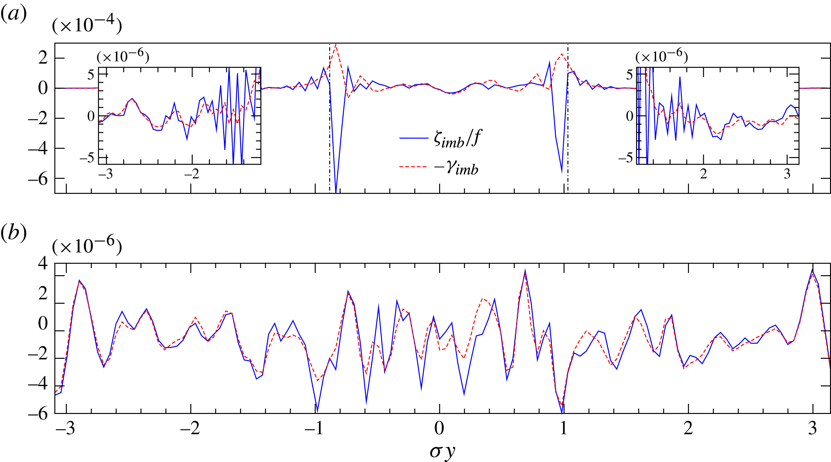
. In fact, for plane-wave solutions of the linearised equations about a state of rest, these two fields exactly cancel. The sum
 ${\it\zeta}_{\mathit{imb}}/f+{\it\gamma}_{\mathit{imb}}$
is indeed much smaller outside the vortex than either field in isolation, as seen in figure 10 displaying one-dimensional cross-sections from the two fields of the cyclone. This confirms that the imbalanced fields mainly consist of IGWs.
One-dimensional cross-sections along
 $y$
of
 ${\it\zeta}_{\mathit{imb}}/f$
(solid) and
 $-{\it\gamma}_{\mathit{imb}}$
(dashed) for the oblate cyclone shown in figure 8. The vertical dot-dashed lines indicate the location of the vortex edge. (a) A transect through the vortex at
 $(x,z)=(-{\it\sigma}^{-1}{\rm\pi}/32,0)$
(insets show regions having much weaker fields). (b) A transect below the vortex at
 $(x,z)=(-{\it\sigma}^{-1}{\rm\pi}/32,-{\rm\pi}/2)$
. The relation
 ${\it\zeta}_{\mathit{imb}}/f+{\it\gamma}_{\mathit{imb}}=0$
satisfied by plane-wave IGWs holds well, verifying that the imbalanced fields mainly consist of IGWs.

The vertical velocity
 $w$
contains only a balanced ageostrophic component
 $w_{\mathit{AGb}}$
and the imbalanced one
 $w_{\mathit{imb}}$
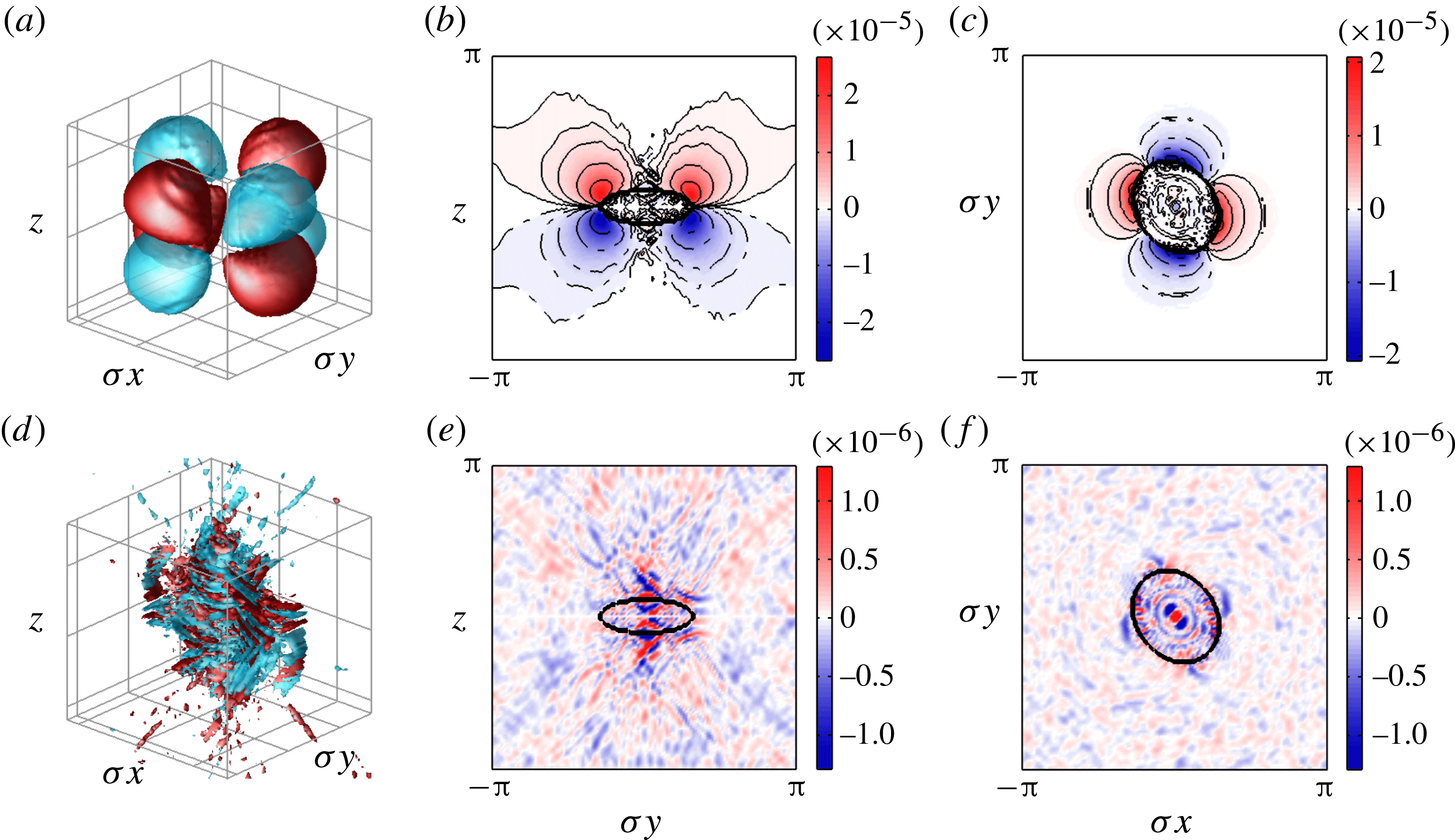
. These are shown in figure 11 (for the cyclone) and figure 12 (for the anticyclone). The balanced component
 $w_{\mathit{AGb}}$
displays a three-dimensional octopolar structure, typical of a rotating ellipsoid around which isopycnals rise and fall antisymmetrically about the midplane
 $z=0$
as the vortex rotates. In
 $w$
, the cyclone exhibits a significantly higher degree of balance, with the magnitude of
 $w_{\mathit{imb}}$
being nearly 10 times smaller than
 $w_{\mathit{AGb}}$
. For the anticyclone, by contrast,
 $w_{\mathit{AGb}}$
and
 $w_{\mathit{imb}}$
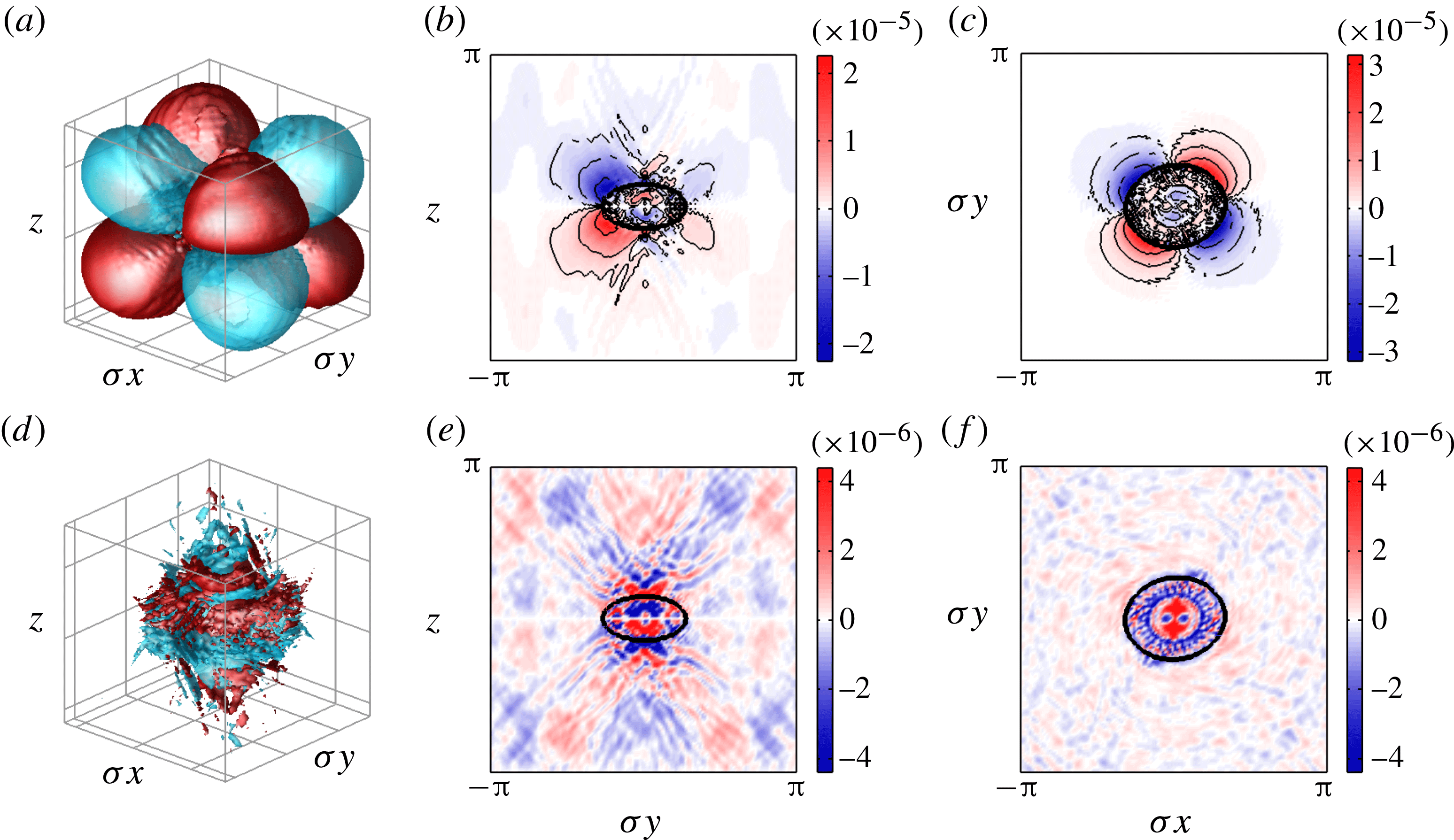
are comparable (note that the colour scales for the imbalanced fields in the figures are nonlinear), and it is evident that OPV balance struggles to clearly define balance. In both flows, waves appear to be trapped inside the vortex, especially in the horizontal cross-sections. Wave crests run approximately perpendicular to the flow at the vortex edge, but become radial approaching the centre of the vortex. While the imbalance is particularly visible here, it nonetheless plays an insignificant role in the flow evolution. This echoes previous findings when care is taken to carefully balance the initial conditions (Dritschel & Viúdez Reference Dritschel and Viúdez2007; McKiver & Dritschel Reference McKiver and Dritschel2008).
The ageostrophic balanced part
 $w_{\mathit{AGb}}$
(a–c) and the imbalanced part
 $w_{\mathit{imb}}$
(d–f) of the vertical velocity associated with a cyclonic oblate vortex (
 $q_{0}=0.25$
,
 ${\it\lambda}_{0}=0.8$
and
 ${\it\mu}_{0}=0.4$
). (a) and (d) show, respectively, three-dimensional surfaces at
 $w_{\mathit{AGb}}=\pm 5\times 10^{-6}$
and
 $w_{\mathit{imb}}=\pm 5\times 10^{-7}$
(positive values are in red); (b) and (e) are vertical
 $y{-}z$
cross-sections at
 $x=-{\it\sigma}^{-1}{\rm\pi}/32$
; (c) and (f) are horizontal
 $x{-}y$
cross-sections at
 $z=-{\rm\pi}/32$
. A nonlinear colour scale is used in the
 $w_{\mathit{imb}}$
cross-section plots. The maximum
 $|w_{\mathit{imb}}|$
is approximately
 $5\times 10^{-6}$
.

As in figure 11, but for an anticyclonic vortex with
 $q_{0}=-0.25$
. Surfaces at
 $w_{\mathit{AGb}}=\pm 5\times 10^{-6}$
and
 $w_{\mathit{imb}}=\pm 2\times 10^{-6}$
are shown in (a) and (d) respectively. A nonlinear colour scale is used in the
 $w_{\mathit{imb}}$
cross-section plots. The maximum
 $|w_{\mathit{imb}}|$
is approximately
 $2\times 10^{-5}$
.

5.3. Prolate vortices
We next compare the fields associated with two highly prolate vortices (
 ${\it\lambda}_{0}=0.7$
,
 ${\it\mu}_{0}=2.4$
and
 $q_{0}=\pm 0.25$
) with the oblate vortices examined just above. These prolate vortices are unstable and undergo mild filament shedding at the top and bottom. At equilibrium,
 $\{\langle {\it\lambda}\rangle ,\langle {\it\mu}\rangle \}=\{0.95,2.21\}$
and
 $\{0.91,2.29\}$
for the cyclone and anticyclone respectively.
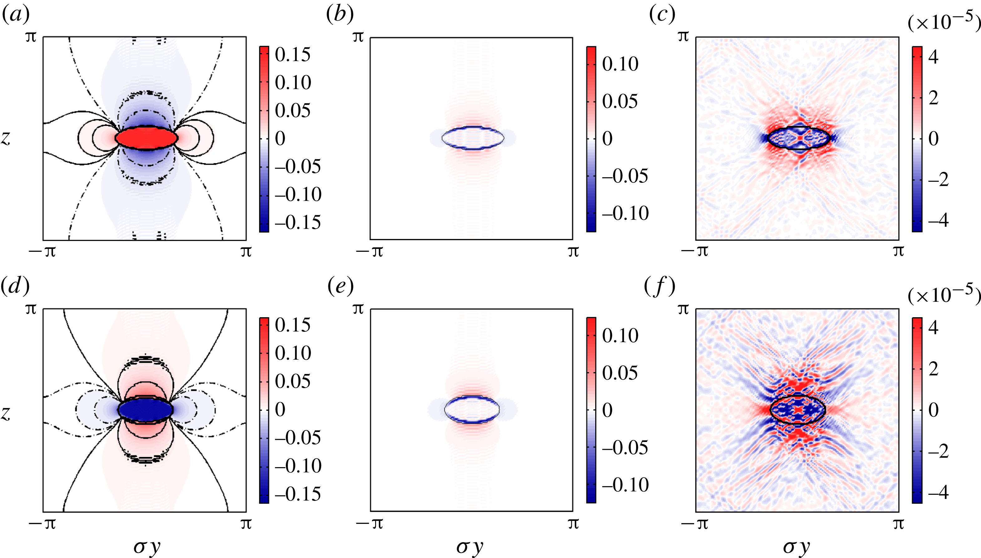
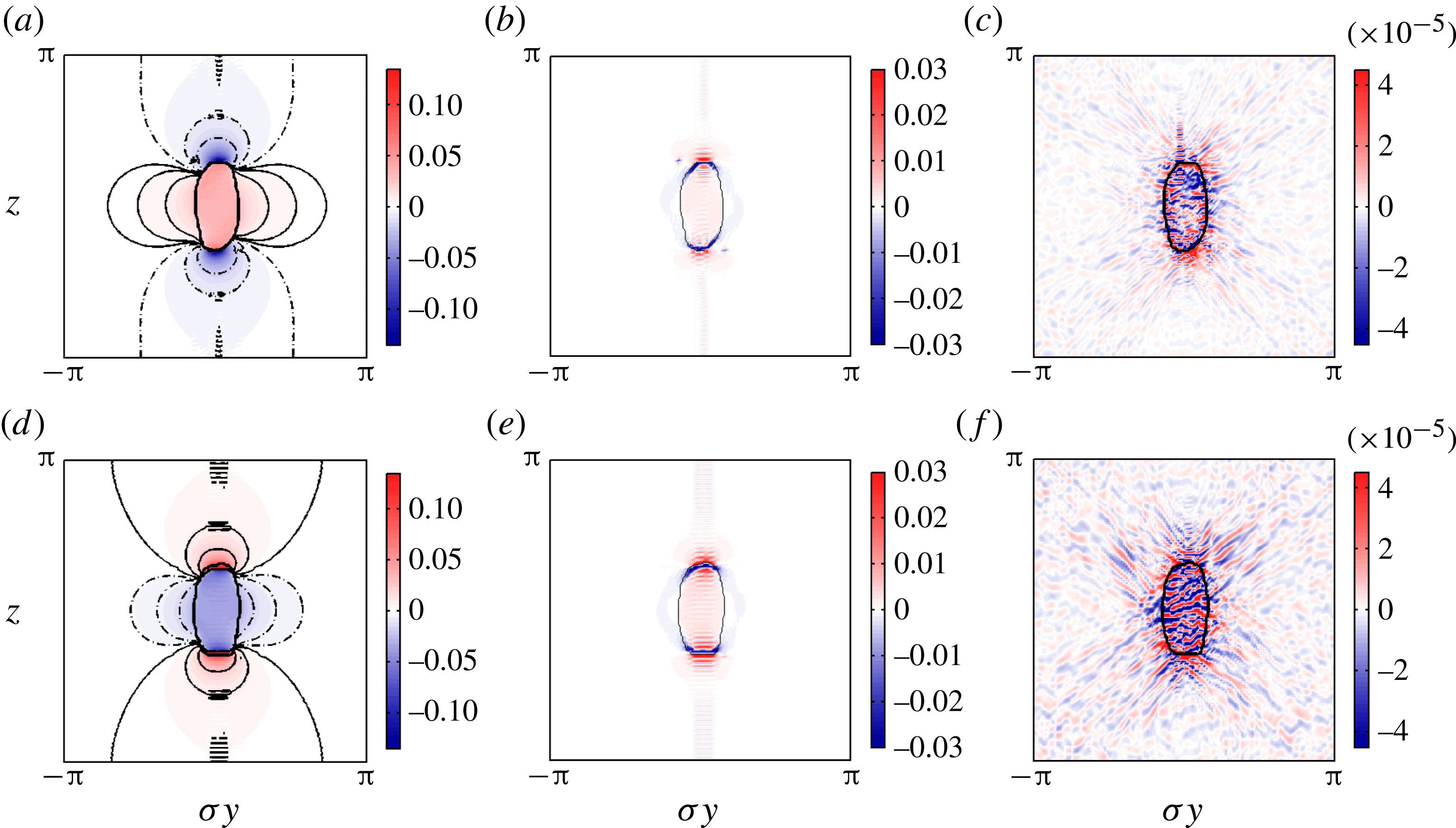
Figure 13 shows components of vertical vorticity,
 ${\it\zeta}_{\mathit{QG}}$
,
 ${\it\zeta}_{\mathit{AGb}}$
and
 ${\it\zeta}_{\mathit{imb}}$
(normalised by
 $f$
), for a cyclone (a–c) and an anticyclone (d–f). Comparing with the oblate vortices in figure 8, we observe broadly similar features, especially in the balanced components. The ageostrophic component again decreases
 ${\it\zeta}$
in the vortex core in both cases, but the decrease is less here due to the more barotropic character of the vortices. The imbalance
 ${\it\zeta}_{\mathit{imb}}$
is also more confined to the vortex interior. In all cases, one sees a characteristic St Andrews cross pattern associated with IGWs emanating from the rotating non-axisymmetric vortex. Note, however, that these waves are exceptionally weak, carrying vorticity nearly
 $10^{3}$
times smaller than the balanced component.
A vertical
 $y{-}z$
cross-section at
 $x=-{\it\sigma}^{-1}{\rm\pi}/32$
of the scaled vertical vorticity
 ${\it\zeta}/f$
for a cyclone (a–c) and an anticyclone (d–f) with
 $q_{0}=\pm 0.25$
respectively. The initial aspect ratios are
 ${\it\lambda}_{0}=0.7$
and
 ${\it\mu}_{0}=2.4$
in both cases. The layout is the same as in figure 8 with the QG balanced part
 ${\it\zeta}_{\mathit{QG}}/f$
in (a) and (d), the ageostrophic balanced part
 ${\it\zeta}_{\mathit{AGb}}/f$
in (b) and (e), and the imbalanced part
 ${\it\zeta}_{\mathit{imb}}/f$
in (c) and (f). The fields are depicted at
 $t=1200T_{\mathit{ip}}$
. A nonlinear colour scale emphasising the weak wave pattern outside the vortex is used for the imbalanced fields. The actual maximum of
 $|{\it\zeta}_{\mathit{imb}}/f|$
is approximately
 $8\times 10^{-4}$
.

Regarding the anomalous static stability
 ${\it\gamma}=b_{z}/N^{2}$
in figure 14, the balanced components are broadly similar to those shown for the oblate vortices in figure 9: QG balance enhances the stability of cyclones and reduces the stability of anticyclones. The ageostrophic component
 ${\it\gamma}_{\mathit{AGb}}$
is insignificant within the vortex and has a minor effect on stability. Regarding the imbalance,
 ${\it\gamma}_{\mathit{imb}}$
has a similar structure to
 ${\it\zeta}_{\mathit{imb}}/f$
, as expected for pure IGWs, and again the imbalance contributes negligibly to the dynamics (
 ${\it\gamma}_{\mathit{imb}}$
is
 $10^{2}$
times smaller than
 ${\it\gamma}_{\mathit{QG}}$
).
As in figure 13, but for the anomalous static stability
 ${\it\gamma}=b_{z}/N^{2}$
, with the QG balanced part
 ${\it\gamma}_{\mathit{QG}}$
in (a) and (d), the ageostrophic balanced part
 ${\it\gamma}_{\mathit{AGb}}$
in (b) and (e), and the imbalanced part
 ${\it\gamma}_{\mathit{imb}}$
in (c) and (f). The top row (a–c) is for the cyclone and the bottom row (d–f) is for the anticyclone. A nonlinear colour scale is used for the imbalanced fields. The maximum
 $|{\it\gamma}_{\mathit{imb}}|$
is approximately
 $2\times 10^{-3}$
.

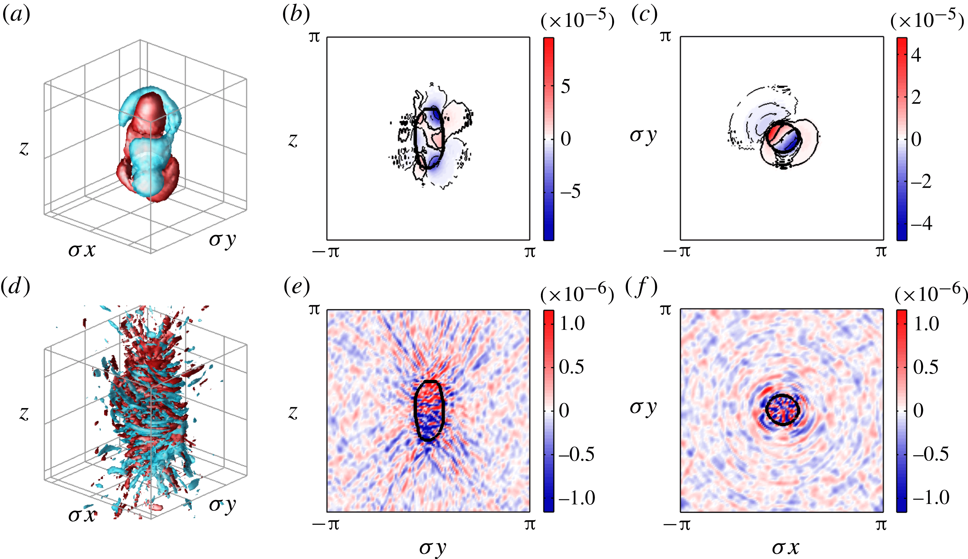
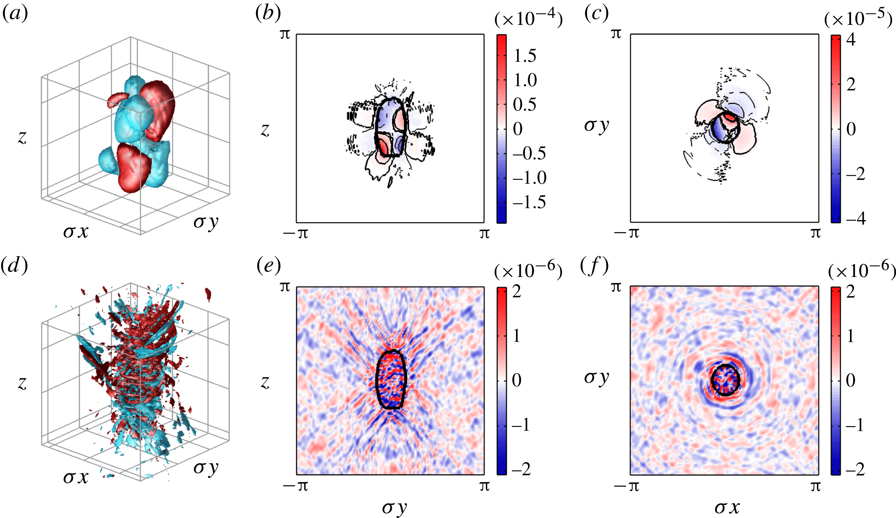
The vertical velocity components
 $w_{\mathit{AGb}}$
and
 $w_{\mathit{imb}}$
, shown in figure 15 (for the cyclone) and in figure 16 (for the anticyclone), are overall significantly different from their oblate-vortex counterparts in figures 11 and 12. First, the ageostrophic component is less well organised and more concentrated in the interior of prolate vortices, perhaps due to fact that vertical motions are less constrained. The pattern is much more complex, especially for the cyclonic state, where no octopolar pattern is evident. The imbalance
 $w_{\mathit{imb}}$
displays the characteristic St Andrews cross pattern in the
 $y{-}z$
cross-section, but in the
 $x{-}y$
cross-section wave crests are seen to be predominantly radial, switching abruptly to azimuthal just outside the vortex boundary. This structure is not seen clearly for the oblate vortices examined, and is probably due to the greater horizontal distortion of the vortex. Finally, as a fraction of
 $w_{\mathit{AGb}}$
, the imbalance
 $w_{\mathit{imb}}$
is appreciably weaker for these prolate vortices compared to their oblate counterparts. Here,
 $w_{\mathit{imb}}$
is 20–30 times smaller than
 $w_{\mathit{AGb}}$
. Even in vertical velocity, these flows exhibit a strong degree of balance.
The ageostrophic balanced part
 $w_{\mathit{AGb}}$
(a–c) and the imbalanced part
 $w_{\mathit{imb}}$
(d–f) of the vertical velocity associated with a cyclonic prolate vortex (
 $q_{0}=0.25$
,
 ${\it\lambda}_{0}=0.7$
and
 ${\it\mu}_{0}=2.4$
). (a) and (d) show, respectively, three-dimensional surfaces at
 $w_{\mathit{AGb}}=\pm 1\times 10^{-5}$
and
 $w_{\mathit{imb}}=\pm 6\times 10^{-7}$
(positive values are in red); (b) and (e) are vertical
 $y{-}z$
cross-sections at
 $x=-{\it\sigma}^{-1}{\rm\pi}/32$
; (c) and (f) are horizontal
 $x{-}y$
cross-sections at
 $z=-{\rm\pi}/32$
. A nonlinear colour scale is used in the
 $w_{\mathit{imb}}$
cross-section plots. The maximum
 $|w_{\mathit{imb}}|$
is approximately
 $4\times 10^{-6}$
.

As in figure 15, but for an anticyclonic vortex with
 $q_{0}=-0.25$
. Surfaces at
 $w_{\mathit{AGb}}=\pm 1\times 10^{-5}$
and
 $w_{\mathit{imb}}=\pm 1.3\times 10^{-6}$
are shown in (a) and (d) respectively. A nonlinear colour scale is used in the
 $w_{\mathit{imb}}$
cross-section plots. The maximum
 $|w_{\mathit{imb}}|$
is approximately
 $7\times 10^{-6}$
.

5.4. Energetics and Rossby number scaling
We next quantify the importance of the balanced and imbalanced parts of the flow using the energy norm
 $$\begin{eqnarray}E_{i}={\textstyle \frac{1}{2}}\langle |\boldsymbol{u}_{i}|^{2}+b_{i}^{2}/N^{2}\rangle ,\end{eqnarray}$$
where
 $i=\mathit{QG}$
,
 $\mathit{AGb}$
or
 $\mathit{imb}$
, and in this section
 $\langle \cdot \rangle$
denotes a domain average. We consider two cases, each having the same initial aspect ratios
 ${\it\lambda}_{0}=0.2$
and
 ${\it\mu}_{0}=2.4$
, but opposite PV,
 $q_{0}=\pm 0.5$
. Also, the simulations are carried out at double the standard resolution in each direction (i.e. at
 $256^{3}$
with subgrid PV kept to scales 16 times finer), and using a time step
 ${\rm\Delta}t=0.075$
. These prolate and initially highly eccentric vortices quickly become unstable and exhibit strong filament shedding between
 $t\approx 200T_{\mathit{ip}}$
and
 $t\approx 1500T_{\mathit{ip}}$
before finally settling down with
 $\{\langle {\it\lambda}\rangle ,\langle {\it\mu}\rangle \}=\{0.90,2.29\}$
and
 $\{0.88,1.73\}$
for the cyclone and anticyclone respectively.
Figure 17 shows the time evolution of the energy ratios
 $E_{\mathit{QG}}/E_{\mathit{tot}}$
,
 $E_{\mathit{AGb}}/E_{\mathit{tot}}$
and
 $E_{\mathit{imb}}/E_{\mathit{tot}}$
where
 $E_{\mathit{tot}}$
is the total energy, found from (5.4) using the full fields
 $\boldsymbol{u}$
and
 $b$
. Notably,
 $E_{\mathit{QG}}>E_{\mathit{tot}}$
and generally increases in time for the cyclone; just the opposite is true for the anticyclone. Hence, QG balance overestimates the energy of cyclones and underestimates that of anticyclones (this has been found to be true generally in all cases examined). We also find that oblate cyclones have larger
 $E_{\mathit{QG}}/E_{\mathit{tot}}\ ({>}1)$
than prolate ones, while oblate anticyclones have smaller
 $E_{\mathit{QG}}/E_{\mathit{tot}}\ ({<}1)$
than prolate ones. In other words, increasing vortex oblateness increases the difference
 $|E_{\mathit{QG}}/E_{\mathit{tot}}-1|$
.
Time evolution of the energy norms
 $E_{\mathit{QG}}$
,
 $E_{\mathit{AGb}}$
and
 $E_{\mathit{imb}}$
(defined in (5.4)) for a cyclone (a–c) and an anticyclone (d–f) at
 $q_{0}=\pm 0.5$
respectively. Both vortices have the same initial aspect ratios,
 ${\it\lambda}_{0}=0.2$
and
 ${\it\mu}_{0}=2.4$
. The insets show the total energy
 $E_{tot}$
versus time.

Turning to the ageostrophic balanced part
 $E_{\mathit{AGb}}$
, this is seen to be just 1–2 % of
 $E_{\mathit{tot}}$
even at these moderately high Rossby numbers.
 $E_{\mathit{AGb}}/E_{\mathit{tot}}$
generally grows in time and appears to level off at late times. Note that two estimates of
 $E_{\mathit{AGb}}$
are provided in the figure, one obtained using OPV balance and the other using NQG balance. Both give closely comparable measures of the small ageostrophic balanced part. Note, simple scaling estimates suggest
 $E_{\mathit{AGb}}/E_{\mathit{tot}}\sim q_{0}^{2}$
(see below), which overestimates the observed energy ratio by more than an order of magnitude if one naively assumes an
 $O(1)$
prefactor in the scaling.
Finally, regarding the imbalanced part
 $E_{\mathit{imb}}$
, first of all it is much smaller than even
 $E_{\mathit{AGb}}$
, with energy ratios of the order
 $10^{-5}$
or smaller.
 $E_{\mathit{imb}}/E_{\mathit{tot}}$
is largest when the vortex undergoes deformation at early times and decays to very small values at late times. Here, one can see a substantial difference between the OPV and NQG estimates of imbalance. Generally, the OPV estimate is about an order of magnitude smaller except during the early period of evolution. In this early period, the flow is rapidly changing due to instability, and OPV struggles to clearly define balance. Indeed, for such time-varying flows, no perfect definition of balance exists; all one can be sure of is that NQG balance provides an overestimate of the imbalance, since presumably one can construct more accurate balance methods for any specific flow situation (cf. Mohebalhojeh & Dritschel Reference Mohebalhojeh and Dritschel2001). OPV balance generally underestimates the imbalance for slowly evolving flows since inevitably some of the imbalance is attributed to the balanced flow, by construction (see appendix D). It is less clear what happens for rapidly evolving flows, but the results of figure 17 indicate that OPV balance overestimates the imbalance in this situation. The upshot is that we can bound the actual level of imbalance below the NQG estimate and above the OPV one, provided the OPV estimate is lower than the NQG one.
We next examine how the QG, balanced ageostrophic and imbalanced energies scale with the PV-based Rossby number
 $q_{0}$
. We consider a single vortex shape with
 ${\it\lambda}_{0}=0.3$
and
 ${\it\mu}_{0}=1.6$
for many different values of
 $q_{0}$
, both positive and negative. We compute
 $E_{\mathit{QG}}$
,
 $E_{\mathit{AGb}}$
and
 $E_{\mathit{imb}}$
at or near the final time in each simulation, when the vortex has reached an equilibrium form. The vortex shape at equilibrium depends on
 $q_{0}$
with
 $0.68<\langle {\it\lambda}\rangle <0.95$
and
 $1.26<\langle {\it\mu}\rangle <1.59$
.
In QG theory, the balanced fields are proportional to
 $q_{0}$
, and hence one would expect
 $E_{\mathit{QG}}$
to scale with
 $q_{0}^{2}$
. The balanced ageostrophic fields are of higher order, and according to the scaling presented in appendix C, one would expect
 $E_{\mathit{AGb}}\sim q_{0}^{4}$
. For the imbalanced fields, the scaling is less clear. What we find is shown in figure 18, plotting the values for
 $E_{\mathit{QG}}$
,
 $E_{\mathit{AGb}}$
and
 $E_{\mathit{imb}}$
as a function of
 $|q_{0}|$
up to
 $|q_{0}|=0.75$
, using circles for cyclonic states (
 $q_{0}>0$
) and crosses for anticyclonic ones (
 $q_{0}<0$
). The QG scaling
 $E_{\mathit{QG}}\sim q_{0}^{2}$
is robust at least up to
 $|q_{0}|=0.5$
, and furthermore
 $E_{\mathit{AGb}}\sim q_{0}^{4}$
over all Rossby numbers considered, with consistently higher values for anticyclones (typically 2–3 times larger). We find that this is generally true for all the vortex shapes in our principal data set (
 $q_{0}=\pm 0.25$
,
 $\pm 0.5$
), implying that, for the same Rossby number magnitude
 $|q_{0}|$
, cyclones are closer to QG balance. The imbalance also exhibits a quartic scaling,
 $E_{\mathit{imb}}\sim q_{0}^{4}$
, albeit with an amplitude
 $10^{4}{-}10^{5}$
times smaller than
 $E_{\mathit{AGb}}$
. There is no clear trend that anticyclones exhibit more imbalance than cyclones except for
 $|q_{0}|\gtrsim 0.5$
. However, we cannot draw a general conclusion based on just one vortex shape (and it is too costly to examine many different vortex shapes in this way).
Log–log plot of the energy norms for the QG, ageostrophic balanced and imbalanced fields, defined in (5.4), versus the PV-based Rossby number
 $q_{0}$
. Circles represent cyclonic states and crosses anticyclonic states. The initial aspect ratios of the vortex are
 ${\it\lambda}_{0}=0.3$
and
 ${\it\mu}_{0}=1.6$
.

5.5. Discussion
In the regime
 $f/N\lesssim 1$
, the concept of ‘balance’, whereby the PV alone determines all dynamical and thermodynamical fields, has proven immensely useful in understanding geophysical fluid behaviour (Hoskins, McIntyre & Robertson Reference Hoskins, McIntyre and Robertson1985; Ford et al.
Reference Ford, McIntyre and Norton2000; Mohebalhojeh & Dritschel Reference Mohebalhojeh and Dritschel2001; McKiver & Dritschel Reference McKiver and Dritschel2008). Balance arises from filtering, in some way, the IGWs from the dynamics. Mathematically, this can be achieved by seeking slowly evolving solutions of the governing equations in which the fluid acceleration
 $\text{D}\boldsymbol{u}/\text{D}t$
is subdominant. This leads to geostrophic and hydrostatic balance to leading order in the Rossby number, proportional to the ratio of the horizontal acceleration to the Coriolis acceleration.
The quasi-geostrophic (QG) model, describing the advection of a linearised approximation of PV by the leading-order geostrophic velocity field on flat isopycnal surfaces, is the simplest dynamical model imposing balance. However, this model does not distinguish cyclonic and anticyclonic flows (apart from the direction of their rotation). Cyclones and anticyclones are mirror images of each other, dynamically. This mirror symmetry is broken once higher-order effects, arising at second order in Rossby number, are taken into account. In fact, QG balance does clearly predict this symmetry breaking, i.e. it provides an estimate of (part of) the ageostrophic flow (Charney Reference Charney1948). It is just that the QG dynamical model does not make use of this (as elaborated below). Indeed it cannot without a further closure assumption (see appendix C).
At the QG level of balance, previous well-known results are confirmed, such as increased inertial stability (closer spacing of vortex lines) in cyclones and the opposite in anticyclones, as well as increased static stability
 ${\it\gamma}$
(closer spacing of density surfaces) in cyclones and the opposite in anticyclones. This already hints at the likely increase in stability with the signed Rossby number
 $q_{0}$
, which has been fully confirmed by our results. QG balance, it is worth emphasising, largely explains the difference in stability between cyclones and anticyclones.
The higher-order ageostrophic balance within the vortex, by contrast, is insignificant. The dominant asymmetry between cyclones and anticyclones is manifest within QG balance. The reason why this asymmetry does not show up in the QG dynamical model is that it is not used: the QG model advects a linearised approximation of PV on flat isopycnal surfaces using purely geostrophic velocities.
Regarding the residual imbalance, consistent with many previous studies of vortex dynamics and turbulence at PV-based Rossby numbers
 ${<}1$
, we find that inertia–gravity waves (the imbalance) play a negligible role, at least when the initial conditions are well prepared to contain minimal imbalance. This explains why we can identify ‘quasi-equilibria’, vortices which persist for long times with very small changes in shape (see Płotka & Dritschel Reference Płotka and Dritschel2014 for analogous results for shallow-water flows). Essentially, the radiation of inertia–gravity waves is too weak to modify the shape of the vortex over any sensible time period (over time periods extending as far as
 $10^{3}$
inertial periods (
 ${\sim}$
days) based on the results presented here).
6. Conclusion
We have examined one of the most basic problems in geophysical fluid dynamics, namely the behaviour of an isolated vortex in uniform background rotation and stratification. It proves especially convenient to consider a vortex having uniform PV since then one can exploit exact steadily rotating solutions having an ellipsoidal shape in the limit of zero Rossby number (vanishingly small PV anomaly relative to the background PV). Properties of these QG ellipsoids are now well known, including their linear stability and many aspects of their nonlinear behaviour. But the restriction to vanishingly small Rossby number is unrealistic in applications to the Earth’s atmosphere and oceans, or to other planetary atmospheres. Our principal aim has been to extend our knowledge of vortex behaviour at finite Rossby number, along the way providing a better understanding of both the limitations and utility of the QG approximation.
The problem investigated principally depends on three parameters, two describing the shape of the vortex (the horizontal and vertical aspect ratios
 ${\it\lambda}$
and
 ${\it\mu}$
), and the dimensionless PV anomaly
 $q_{0}$
within the vortex (the Rossby number). The problem also depends on the Coriolis to buoyancy frequency ratio
 $f/N$
, but only weakly when
 $f/N\lesssim 1$
(Smyth & McWilliams Reference Smyth and McWilliams1998; Dritschel & McKiver Reference Dritschel and McKiver2014). The regime of small
 $f/N$
is widely applicable to commonly occurring geophysical flows.
We have examined the stability of vortices covering a wide range of initial shapes
 $({\it\lambda}_{0},{\it\mu}_{0})$
and Rossby numbers
 $q_{0}$
. We have systematically catalogued the wide variety of instabilities which may occur (figure 3), and have identified the quasi-stable equilibrium configurations emerging from these instabilities (figure 4). For these configurations, we have shown that their rotation rate
 ${\it\Omega}$
depends primarily on the late-time average value of
 ${\it\mu}$
and
 $q_{0}$
(figure 6) and that anticyclones rotate faster than cyclones of the same general shape and
 $|q_{0}|$
. This asymmetry was explained using a higher-order balanced model, and was shown to stem from ageostrophic effects at
 $O(q_{0}^{2})$
.
We have carefully analysed the nature of balance, or the degree to which the PV field alone determines the instantaneous flow. We have shown explicitly that the residual imbalance, characterised by inertia–gravity waves, is negligible across the entire parameter space investigated. The vortex motion depends almost exclusively on the balanced dynamics. Decomposing this into a leading-order QG part and a remaining (balanced) ageostrophic part, we have shown that the gross stability properties of the vortices depend primarily on QG balance, not on the higher-order ageostrophic balance. In other words, the simplest balance – QG balance – is sufficient to explain why cyclones are generally more stable than anticyclones. While this result is not new, our work is the first comprehensive demonstration of it.
In the present work, we have restricted attention to small frequency ratios
 $f/N$
. A next step would be to study the changes to vortex behaviour that take place for increasing
 $f/N$
, at least up to
 $O(1)$
values, keeping the shape and the Rossby number
 $q_{0}$
of the vortex (or family of vortices) fixed. In rotating stratified turbulence (Dritschel & McKiver Reference Dritschel and McKiver2014) however, no significant changes have been found to occur in the basic flow properties for
 $|q_{0}|\lesssim 1$
for
 $f/N$
up to one, consistent with the results of Smyth & McWilliams (Reference Smyth and McWilliams1998) who studied the stability of a columnar vortex.
Open questions remain for
 $|q_{0}|\gtrsim 1$
that are inaccessible to the approach taken here. Reducing
 $q_{0}$
much below
 $-0.5$
greatly enhances the possibility of inertial instability, and under these circumstances one would expect a violent break-up of the vortex (Smyth & McWilliams Reference Smyth and McWilliams1998). Increasing
 $q_{0}$
above one would appear to eventually lead to inertial and/or static instability, if one can extrapolate the trends exhibited by the ageostrophic balanced fields in figures 13 and 14, for example. As the ageostrophic balanced fields grow quadratically with
 $q_{0}$
while the QG fields only grow linearly, there may exist a
 $q_{0}$
sufficiently large when static, inertial or another form of instability occurs (see appendix A.2 in Dritschel & Viúdez Reference Dritschel and Viúdez2003).
A problem which affects this research and related fundamental studies of vortex dynamics is the present lack of comprehensive observational data. Few ocean vortices, for example, have been analysed in detail (and very little is known about their PV structure), and these few vortices cannot be assumed to be representative. Surface observations alone do not provide vertical structure information, and miss out vortices at depth. Observational analyses are costly and we are not likely to obtain a representative cross-section of ocean vortex properties in the near future. What is more promising in the interim is an analysis of ocean vortex properties in high-resolution global simulations of the oceans. This would provide much needed support for theoretical studies, and moreover can be done now.
Acknowledgements
We are indebted to X. Carton for his insightful discussions with us. Support for this research has come from the UK Engineering and Physical Sciences Research Council (grant number EP/H001794/1).
Appendix A. The equivalent oriented ellipsoid
Given a volume
 $\mathscr{V }$
with uniform PV anomaly
 $q$
, we can compute its zeroth-, first- and second-order spatial moments, denoted by
 $V$
,
 $\bar{x}_{i}$
and
 $I_{ij}$
respectively, from the following expressions:
 $$\begin{eqnarray}\displaystyle & \displaystyle V=\int _{\mathscr{V }}\text{d}\boldsymbol{x}, & \displaystyle\end{eqnarray}$$
 $$\begin{eqnarray}\displaystyle & \displaystyle \bar{x}_{i}=\frac{1}{V}\int _{\mathscr{V }}x_{i}\text{d}\boldsymbol{x}, & \displaystyle\end{eqnarray}$$
 $$\begin{eqnarray}\displaystyle & \displaystyle I_{ij}=\frac{1}{V}\int _{\mathscr{V }}\left(\tilde{x}_{i}\,\tilde{x}_{j}-\frac{{\it\delta}_{ij}}{3}\,\mathop{\sum }_{l=1}^{3}\tilde{x}_{l}^{\,2}\right)\text{d}\boldsymbol{x}. & \displaystyle\end{eqnarray}$$
 $\boldsymbol{x}=(x_{1},x_{2},x_{3})=(x,y,z)$
denotes the position vector,
 $\tilde{\boldsymbol{x}}=\boldsymbol{x}-\bar{\boldsymbol{x}}$
is the position vector relative to the vortex centre at
 $\bar{\boldsymbol{x}}$
, and
 ${\it\delta}_{ij}$
is the Kronecker delta symbol. Note that there are only nine independent moments in (A 1) since
 $\sum _{i}I_{ii}=0$
.
We define an equivalent oriented ellipsoid
 $\mathscr{E}$
as one that has the same moments as the vortex up to the second order. This definition slightly differs from the usual one (Chandrasekhar Reference Chandrasekhar1987) in that we require the ellipsoid to have the same volume as the vortex. Now, a quadric surface, including the ellipsoid, centred at
 $\boldsymbol{x}^{\prime }$
is represented by the following general equation of second degree:
 $$\begin{eqnarray}(\boldsymbol{x}-\boldsymbol{x}^{\prime })^{\text{T}}\,\unicode[STIX]{x1D63C}^{-1}\,(\boldsymbol{x}-\boldsymbol{x}^{\prime })=1,\end{eqnarray}$$
where
 $\unicode[STIX]{x1D63C}$
is a symmetric
 $3\times 3$
matrix. For the equivalent oriented ellipsoid, it is obvious that
 $\boldsymbol{x}^{\prime }=\bar{\boldsymbol{x}}$
. To see the relation between
 $A_{ij}$
and
 $I_{ij}$
, let
 $V_{\mathscr{E}}$
be the volume of
 $\mathscr{E}$
,
 $a_{i}$
be its semi-axis length in the
 $x_{i}$
-direction and
 $\unicode[STIX]{x1D64D}$
be the rotation matrix with the property
 $$\begin{eqnarray}\unicode[STIX]{x1D64D}^{\text{T}}\unicode[STIX]{x1D63C}^{-1}\unicode[STIX]{x1D64D}=\unicode[STIX]{x1D63F}=\left[\begin{array}{@{}ccc@{}}a_{1}^{-2} & 0 & 0\\ 0 & a_{2}^{-2} & 0\\ 0 & 0 & a_{3}^{-2}\end{array}\right].\end{eqnarray}$$
We compute the second moments of
 $\mathscr{E}$
by transforming
 $\mathscr{E}$
into the unit sphere
 $\mathscr{S}$
centred at the origin. This is achieved by the translation
 $\boldsymbol{x}-\boldsymbol{x}^{\prime }$
followed by the rotation
 $\unicode[STIX]{x1D64D}$
. We finally scale length by
 $a_{i}$
along the principal axes:
 ${\it\xi}_{k}=a_{k}^{-1}\sum _{i}\!R_{ki}(x_{i}-x_{i}^{\prime })$
. Hence,
 $$\begin{eqnarray}\displaystyle \frac{1}{V_{\mathscr{E}}}\int _{\mathscr{E}}(x_{i}-x_{i}^{\prime })(x_{j}-x_{j}^{\prime })\text{d}\boldsymbol{x} & = & \displaystyle \frac{a_{1}a_{2}a_{3}}{V_{\mathscr{E}}}\mathop{\sum }_{kl}R_{ik}\left[(a_{k}a_{l})\int _{\mathscr{S}}{\it\xi}_{k}{\it\xi}_{l}\text{d}{\bf\xi}\right]R_{lj}^{\text{T}}\nonumber\\ \displaystyle & = & \displaystyle \frac{1}{5}\mathop{\sum }_{kl}R_{ik}D_{kl}^{-1}R_{lj}^{\text{T}}=\frac{A_{ij}}{5}.\end{eqnarray}$$
Above, the factor
 $a_{1}a_{2}a_{3}$
is the Jacobian associated with the rotation, and the integral over
 $\mathscr{S}$
equals
 $4{\rm\pi}{\it\delta}_{kl}/15$
. By the definition of equivalent oriented ellipsoid, we thus have
 $$\begin{eqnarray}A_{ij}-\frac{{\it\delta}_{ij}}{3}\mathop{\sum }_{l}A_{ll}=5I_{ij}.\end{eqnarray}$$
The shape and orientation of the ellipsoid can then be deduced from the eigenvalues and eigenvectors of
 $\unicode[STIX]{x1D63C}$
(see e.g. McKiver & Dritschel Reference McKiver and Dritschel2003 for a straightforward derivation).
Appendix B. Estimation of instantaneous vortex rotation rate
In this appendix, we present a method to estimate the vortex rotation rate from the velocity field at a single time instant. This method is used when the rotation rate, for example
 ${\it\Omega}_{0}$
at
 $t=0$
, cannot be obtained by tracking the rotation of the equivalent ellipsoid. The strategy is to find an optimal co-rotating frame in which the vortex shape appears to be least unsteady, and to identify the angular velocity
 ${\it\Omega}$
of this frame as the vortex rotation rate. The vortex shape is delineated by the PV contours andif a PV contour
 $\mathscr{C}_{l}$
on an isopycnal surface is steady, the velocity on
 $\mathscr{C}_{l}$
is tangent to
 $\mathscr{C}_{l}$
. Hence, to represent the unsteadiness, we compute the square of the non-tangential component of the velocity integrated around all contours in a rotating frame and summed over all surfaces:
 $$\begin{eqnarray}\mathscr{F}({\it\Omega})=\mathop{\sum }_{l}\oint _{\mathscr{C}_{l}}|\boldsymbol{u}^{\prime }-(\boldsymbol{u}^{\prime }\boldsymbol{\cdot }\hat{\boldsymbol{e}}_{t})\hat{\boldsymbol{e}}_{t}|^{2}\text{d}s.\end{eqnarray}$$
Here
 $\boldsymbol{u}^{\prime }=\boldsymbol{u}+{\it\Omega}\boldsymbol{a}$
(with
 $\boldsymbol{a}\equiv (y,-x,0)$
) is the velocity in the rotating frame and
 $\hat{\boldsymbol{e}}_{t}$
is the unit tangent vector along
 $\mathscr{C}_{l}$
. We seek
 ${\it\Omega}$
by minimising
 $\mathscr{F}({\it\Omega})$
; therefore, setting
 $\text{d}\mathscr{F}/\text{d}{\it\Omega}=0$
gives
 $$\begin{eqnarray}{\it\Omega}=-\frac{\displaystyle \mathop{\sum }_{l}\oint _{\mathscr{C}_{l}}\left[\,\boldsymbol{u}\boldsymbol{\cdot }\boldsymbol{a}-(\boldsymbol{u}\boldsymbol{\cdot }\hat{\boldsymbol{e}}_{t})(\boldsymbol{a}\boldsymbol{\cdot }\hat{\boldsymbol{e}}_{t})\,\right]\text{d}s}{\displaystyle \mathop{\sum }_{l}\oint _{\mathscr{C}_{l}}\left[\,|\boldsymbol{a}|^{2}-(\boldsymbol{a}\boldsymbol{\cdot }\hat{\boldsymbol{e}}_{t})^{2}\,\right]\text{d}s}.\end{eqnarray}$$
This method works well when the system consists of a single well-defined vortex (which is the case at
 $t=0$
). As the vortex evolves in time, filaments and satellites may be spun off, and tracking the equivalent ellipsoid becomes the preferred method.
Appendix C. Nonlinear quasi-geostrophic balance
Consider a rotating stratified fluid described by (2.10) with the definitions of
 $\boldsymbol{A}_{h}$
and
 $q$
given by (2.9) and (2.16) respectively. Introduce the small parameter
 ${\it\epsilon}\equiv \text{max}|q|$
and recall
 ${\it\sigma}=f/N$
. Using the standard QG scalings
 $$\begin{eqnarray}t\sim {\it\epsilon}^{-1},\quad (u,v)\sim {\it\epsilon},\quad w\sim {\it\sigma}{\it\epsilon}^{2},\quad b\sim {\it\sigma}{\it\epsilon}\end{eqnarray}$$
motivates the following expansions of the components of the vector potential
 ${\bf\varphi}=({\it\varphi},{\it\psi},{\it\phi})$
:
 $$\begin{eqnarray}\displaystyle & \displaystyle {\it\phi}={\it\epsilon}{\it\phi}_{1}+{\it\epsilon}^{2}{\it\phi}_{2}+O({\it\epsilon}^{3}), & \displaystyle\end{eqnarray}$$
 $$\begin{eqnarray}\displaystyle & \displaystyle {\bf\varphi}_{h}={\it\epsilon}^{2}{{\bf\varphi}_{h}}_{2}+O({\it\epsilon}^{3}). & \displaystyle\end{eqnarray}$$
 ${\it\epsilon}$
,
 $$\begin{eqnarray}q=({\rm\nabla}_{h}^{2}+{\it\sigma}^{2}\partial _{zz}){\it\phi}_{1},\end{eqnarray}$$
except that here
 $q$
is the exact Rossby–Ertel PV anomaly. At order
 ${\it\epsilon}^{2}$
, we obtain a system of linear constant-coefficient equations for the second-order potentials:
 $$\begin{eqnarray}\displaystyle & \displaystyle {\it\sigma}^{-2}({\rm\nabla}_{h}^{2}+{\it\sigma}^{2}\partial _{zz}){\it\varphi}_{2}+(1-{\it\sigma}^{-2})(\partial _{xx}{\it\varphi}_{2}+\partial _{xy}{\it\psi}_{2})=-2J_{yz}(\partial _{x}{\it\phi}_{1},\partial _{y}{\it\phi}_{1}), & \displaystyle\end{eqnarray}$$
 $$\begin{eqnarray}\displaystyle & \displaystyle {\it\sigma}^{-2}({\rm\nabla}_{h}^{2}+{\it\sigma}^{2}\partial _{zz}){\it\psi}_{2}+(1-{\it\sigma}^{-2})(\partial _{xy}{\it\varphi}_{2}+\partial _{yy}{\it\psi}_{2})=-2J_{zx}(\partial _{x}{\it\phi}_{1},\partial _{y}{\it\phi}_{1}), & \displaystyle\end{eqnarray}$$
 $$\begin{eqnarray}\displaystyle & \displaystyle {\it\sigma}^{-2}({\rm\nabla}_{h}^{2}+{\it\sigma}^{2}\partial _{zz}){\it\phi}_{2}+(1-{\it\sigma}^{-2})(\partial _{xz}{\it\varphi}_{2}+\partial _{yz}{\it\psi}_{2})=0. & \displaystyle\end{eqnarray}$$
 $J_{yz}(F,G)=\partial _{y}F\,\partial _{z}G-\partial _{z}F\,\partial _{y}G$
with
 $J_{zx}(F,G)$
analogously defined. The third equation (C 4c
) in this set incorporates a constraint needed to close the equations at second order, namely that the second-order potentials make no contribution to the PV at order
 ${\it\epsilon}^{2}$
. For a given PV anomaly
 $q$
at any instant of time, the NQG system can be solved for
 ${\it\phi}_{1}$
and
 ${\bf\varphi}_{2}$
iteratively. The velocity and the buoyancy fields can then be obtained from (2.13) and (2.14) respectively.
Appendix D. Optimal potential vorticity balance
For simplicity, consider a given PV field represented by a single contour
 $C^{\ast }$
of PV value
 $q^{\ast }$
. The objective of OPV balance is to find a potential
 ${\bf\varphi}^{\ast }(\boldsymbol{x})$
such that the target balanced flow specified by
 $\{C^{\ast },{\bf\varphi}^{\ast }\}$
has minimum IGW emission. This is achieved, approximately, using the iterative backwards–forwards time integration cycle introduced in Viúdez & Dritschel (Reference Viúdez and Dritschel2004). During each cycle, the PV value on the contour changes according to
 $$\begin{eqnarray}q(t)=q^{\ast }\sin ^{2}\left(\frac{{\rm\pi}t}{2{\it\tau}}\right).\end{eqnarray}$$
At
 $t=0$
, the system is in a state of rest. The idea is to very slowly ramp up
 $q(t)$
while evolving the full set of equations to minimise the emission of IGWs. As a result, the system at
 $t={\it\tau}$
represents an estimate of the target balanced state.
Schematic of the OPV balance procedure. At the beginning of the
 $n$
th iteration, the contour
 $C_{n}$
is reset to
 $C^{\ast }$
. The system is then integrated backwards in time from
 ${\it\tau}$
to 0 while the PV is ramped down from
 $q^{\ast }$
to 0 according to (D 1). Since
 $q(0)=0$
,
 ${\bf\varphi}_{n}(\boldsymbol{x},0)$
contains only the imbalance, which is removed by setting
 ${\bf\varphi}_{n}(\boldsymbol{x},0)=0$
. Then, a forwards integration from
 $t=0$
to
 $t={\it\tau}$
with the PV being ramped up from 0 to
 $q^{\ast }$
produces the potential
 ${\bf\varphi}_{n+1}(\boldsymbol{x},{\it\tau})$
for the next iteration. To start the cycle, the ‘frozen’ initialisation (see text) is used to supply an initial guess
 ${\bf\varphi}_{0}(\boldsymbol{x},{\it\tau})$
. The procedure is said to converge when
 $|{\bf\varphi}_{n}(\boldsymbol{x},{\it\tau})-{\bf\varphi}_{n-1}(\boldsymbol{x},{\it\tau})|$
is sufficiently small. We then have the desired potential
 ${\bf\varphi}^{\ast }={\bf\varphi}_{n}$
.

The cycle starts at
 $t={\it\tau}$
with the PV contour
 $C({\it\tau})=C^{\ast }$
and some
 ${\bf\varphi}(\boldsymbol{x},{\it\tau})$
which is an estimate of the target potential
 ${\bf\varphi}^{\ast }(\boldsymbol{x})$
. To improve the estimate, we integrate the system
 $C(t)$
and
 ${\bf\varphi}(\boldsymbol{x},t)$
backwards in
 $t$
, letting
 $C(t)$
vary as the flow distorts it. Upon arriving at
 $t=0$
,
 $q(0)=0$
but we generally find
 ${\bf\varphi}(\boldsymbol{x},0)\neq 0$
. This indicates that we have not yet converged. We reset
 ${\bf\varphi}(\boldsymbol{x},0)=0$
and integrate forward from a state of rest. Upon arriving at
 $t={\it\tau}$
, we have an improved estimate of
 ${\bf\varphi}^{\ast }(\boldsymbol{x})$
in
 ${\bf\varphi}(\boldsymbol{x},{\it\tau})$
but now
 $C({\it\tau})$
will generally not coincide with
 $C^{\ast }$
. We reset
 $C({\it\tau})=C^{\ast }$
and integrate backwards again and so on. The cycle ends when the difference between
 ${\bf\varphi}(\boldsymbol{x},{\it\tau})$
at two successive iterations is smaller than some prescribed tolerance.
To start the cycle described above, we need an initial estimate
 ${\bf\varphi}(\boldsymbol{x},{\it\tau})$
in the first iteration. This is obtained as follows. Starting with a state of rest at
 $t=0$
, we ‘freeze’
 $C(t)=C^{\ast }$
for all
 $t$
and integrate the remaining equations forward to
 $t={\it\tau}$
to get a first guess for
 ${\bf\varphi}(\boldsymbol{x},{\it\tau})$
.
Figure 19 describes the OPV procedure schematically. As shown in Viúdez & Dritschel (Reference Viúdez and Dritschel2004), convergence is generally exponentially fast except when
 ${\it\tau}$
is taken to be too large. Here, we take
 ${\it\tau}=4T_{\mathit{ip}}$
, which works well in most cases and is consistent with the suggested choice in Viúdez & Dritschel (Reference Viúdez and Dritschel2004).