


1 Introduction
In a vast array of both industrial and natural situations, fluid flows transport small particulate matter that is not neutrally buoyant. Due to its widespread applications, then, the question of how such ‘weakly inertial’ particles are transported in both turbulent (Guha Reference Guha2008) and laminar (Leal Reference Leal1980) flows has been a very active topic of research. The dynamics of such particles is highly complex, because they do not in general move in the same way as an equivalently sized fluid element would – they experience different forces, and may even eventually settle out. For spherical inertial particles, the response time scale of the particles relative to the time scale of the smallest fluid motions, a ratio known as the Stokes number, dictates the degree to which particles follow the flow. For nearly inertialess particles (that is, those with small Stokes and particle Reynolds numbers), these differences may be small when evaluating velocities at a single instant; but when predicting long-time particle transport, there may be an integrated effect that can result in larger discrepancies even in this limit (Ouellette, O’Malley & Gollub Reference Ouellette, O’Malley and Gollub2008).
When finite-sized particles are additionally not spherical, their dynamics can be further influenced by orientation-dependent lift and drag forces. Thus, the way that the shape of particles couples to their rotational and translational dynamics is an emerging area of interest (Andersson & Soldati Reference Andersson and Soldati2013; Voth & Soldati Reference Voth and Soldati2017). Much of this research has explored the rotational dynamics of rods and prolate spheroids in turbulence; for examples, see Shin & Koch (Reference Shin and Koch2005), Pumir & Wilkinson (Reference Pumir and Wilkinson2011), Parsa et al. (Reference Parsa, Calzavarini, Toschi and Voth2012), Ni, Ouellette & Voth (Reference Ni, Ouellette and Voth2014). A growing body of work, however, has addressed a broader spectrum of anisotropic-particle shapes, with again focus on characterizing particle rotational dynamics in isotropic turbulence via models (Klett Reference Klett1995) and simulations (Byron et al. Reference Byron, Einarsson, Gustavsson, Voth, Mehlig and Variano2015) and in shear flows (Challabotla, Zhao & Andersson Reference Challabotla, Zhao and Andersson2015a ). Inertia is often neglected in these simulations, which led Einarsson, Angilella & Mehlig (Reference Einarsson, Angilella and Mehlig2014) to analyse how weak inertia may affect some of these orientational dynamics findings. This focus on rotation is partly due to the symmetries of isotropic turbulence, so that long-time transport is not necessarily expected to be affected by particle orientation, and to the fact that the rotational and translational degrees of freedom for an anisotropic but non-chiral particle are not expected to be coupled (Brenner Reference Brenner1964).
In many cases, however, there is the possibility that the flow itself may break this symmetry and couple particle shape to transport. Our particular motivating case is that of the fate of microplastic particles in the ocean. Microplastics, a persistent and growing source of contamination in our oceans (Van Sebille et al. Reference Van Sebille, Wilcox, Lebreton, Maximenko, Hardesty, Van Franeker, Eriksen, Siegel, Galgani and Law2015), are typically defined to be small irregularly shaped plastic particles with length scales of less than 5 mm. Their most typical forms are elongated and fibrous, flat and planar fragments (Chubarenko et al. Reference Chubarenko, Bagaev, Zobkov and Esiukova2016), or nearly spherical pellets (Ryan et al. Reference Ryan, Moore, van Franeker and Moloney2009). Thus, to a good approximation, they can be idealized as particles along the spheroidal spectrum, from discs to spheres to rods. Such an approximation is additionally justified given that simplifying complex shapes to spheroids has been proven as an effective modelling technique by Bretherton (Reference Bretherton1962). Microplastic mass densities are close to that of water, but may be either positively or negatively buoyant. Most efforts to model microplastic transport in the ocean, however, treat the particles as tracers (Maximenko, Hafner & Niiler Reference Maximenko, Hafner and Niiler2012), potentially with a superimposed constant settling velocity (Kukulka et al. Reference Kukulka, Proskurowski, Morét-Ferguson, Meyer and Law2012), or neglect any effects of their shape and instead prescribe only bulk properties to the modelled particles (Beron-Vera, Olascoaga & Lumpkin Reference Beron-Vera, Olascoaga and Lumpkin2016). Although this latter approach may be more accurate than treating microplastics as pure flow tracers, neglecting particle shape effects has been shown to result in errors in predictions of anisotropic-particle transport (Broday et al. Reference Broday, Fichman, Shapiro and Gutfinger1997).
Most plastic pollution in the ocean is land sourced, and many delicate ecosystems reside near shorelines. Thus, understanding the transport of microplastics in the near-shore environment is a key environmental problem. The transport of scalars in the near-shore, coastal zone is controlled by phenomena such as wind waves, turbulence, Langmuir cells, longshore currents, rip currents and tidal currents. These complex and interacting hydrodynamic phenomena influence transport in these areas. Here, however, we simplify the problem and examine one simple but ubiquitous aspect of the near-shore environment: surface gravity waves. While linear wave theory predicts that fluid elements trace orbits as the wave passes, surface gravity waves also generate a mean Lagrangian current or Stokes drift (Stokes Reference Stokes1851). This induced current has well-studied effects on large-scale transport and mixing processes in the ocean as it interacts with other forces. For example, the Coriolis–Stokes forcing can induce opposing flow (Hasselmann Reference Hasselmann1970), and the Stokes vortex force describes how wind shear produces Langmuir circulation (Leibovich Reference Leibovich1983; McWilliams, Sullivan & Moeng Reference McWilliams, Sullivan and Moeng1997). When diffusion of particles is also included, a non-zero mean drift velocity appears even in the case where classical Stokes drift would vanish; this has been termed stochastic Stokes drift (Jansons & Lythe Reference Jansons and Lythe1998). Stokes drift has also been shown to be an important mechanism for modelling the transport of microplastics in the coastal oceans (Isobe et al. Reference Isobe, Kubo, Tamura, Kako, Nakashima and Fujii2014). Less is known, however, about how weakly inertial, anisotropic particles behave in these wavy flows.
The mean transport of particles in internal gravity waves was studied by Grinshpun et al. (Reference Grinshpun, Redcoborody, Kravchuk, Zadorozhnii and Zhdanov2000), who examined Stokes drag on particles that were essentially inertialess. However, as discussed above, inertial particles feel other forces as well. Previous studies that modelled the transport of finite-sized spherical particles under surface gravity waves found that added mass must be included (Eames Reference Eames2008) as well as other inertial effects (Santamaria et al. Reference Santamaria, Boffetta, Afonso, Mazzino, Onorato and Pugliese2013). The properties of the waves themselves can also lead to different results (Bakhoday-Paskyabi Reference Bakhoday-Paskyabi2015). Even though these models are very simple, they show that inertial particle transport in waves is both non-trivial and not well understood.
Here, we bring together these various threads of research and study the effects of shape and weak inertia on the orientation and transport of particles in wavy flows. We conducted numerical simulations of anisotropic, inertialess and weakly inertial spheroids in an analytically specified wave field. We find that the particles adopt preferential orientations relative to the wave propagation direction that are purely a function of their aspect ratio; and that this preferential alignment in turn leads to differences in the downstream transport of the particles. Thus, the interaction of the flow field and the particle dynamics leads to a coupling between the particle shape and their net transport. We also find that the rate of approach to this preferred alignment depends on the initial particle orientation, so that a plume of randomly oriented anisotropic particles will experience dispersion as it is advected downstream. Our results demonstrate that particle shape is a key component for predicting transport in wavy flows and should be included in models of the dispersal of oceanic microplastics.
We begin below in § 2 by describing our model for both the particles and the flow. In § 3, we present our results, focusing separately on the particle orientation, transport and dispersion. We also consider the contribution of the wavy oscillation in addition to the residual Stokes drift velocity field. Finally, in § 4, we summarize our results and discuss the potential contributions of effects we have not considered in our model.
2 Methodology
2.1 Particle model
Characteristics of particles used in the simulations. Both a prolate and oblate spheroidal particle and their corresponding diameters and symmetry axis in the coordinate system are shown. The waves lie in the
 $x$
–
 $z$
plane and move in the positive
 $x$
direction; they are not shown to scale. The particle’s orientation is described by the unit vector
 $p_{i}$
, which lies along the particle’s axis of symmetry.

We simulated particle trajectories using a point-particle approach to isolate the effects of particle shape on transport. The modelled particles are spheroids, and are described by
 $d_{s}$
, the diameter of the equivalent sphere with the same volume as the spheroid, and
 ${\mathcal{E}}$
, the eccentricity. We define
 ${\mathcal{E}}$
as
 $(\unicode[STIX]{x1D706}^{2}-1)/(\unicode[STIX]{x1D706}^{2}+1)$
, where
 $\unicode[STIX]{x1D706}$
is the aspect ratio and is given by the ratio
 $a/b$
, where
 $a$
is the length along the particle’s axis of symmetry and
 $b$
is the length of one of the orthogonal axes, as shown in figure 1. We considered both oblate (
 ${\mathcal{E}}<0$
) and prolate (
 ${\mathcal{E}}>0$
) spheroids. Note that
 ${\mathcal{E}}=0$
for a sphere, and that the limiting cases of
 ${\mathcal{E}}\rightarrow \pm 1$
correspond to rods and discs, respectively.
We ran simulations both with and without consideration of particle inertia. As described below, neglecting inertia allows us to isolate the interaction between the wave-driven flow and the particle orientation, whereas simulations with inertia allow the characterization of the effect of the orientation on particle transport.
In the inertialess limit, the particles follow fluid-element trajectories, although their orientation gives them additional degrees of freedom. Their rotation is governed by Jeffery’s (Reference Jeffery1922) equation for a spheroid, given by
 $$\begin{eqnarray}{\dot{p}}_{i}=\unicode[STIX]{x1D6FA}_{ij}p_{j}+{\mathcal{E}}(\unicode[STIX]{x1D61A}_{ij}p_{j}-p_{i}p_{j}\unicode[STIX]{x1D61A}_{jl}p_{l}),\end{eqnarray}$$
where
 $\unicode[STIX]{x1D6FA}_{ij}$
and
 $\unicode[STIX]{x1D61A}_{ij}$
are the anti-symmetric and symmetric parts of the fluid velocity gradient tensor and
 $p_{i}$
is a unit vector pointing along the particle’s axis of symmetry, as shown in figure 1.
When particle inertia is included, both the orientation and trajectory of the particle must be considered, since the particles no longer follow the flow. We assumed one-way coupling between the fluid and the particles, so that there is no back reaction of the particles on the flow; we also ignored particle–particle interactions and collisions. We also only considered the low particle Reynolds number regime. We define the particle Reynolds number
 $Re_{p}$
to be
 $Re_{p}=|v-u|d/\unicode[STIX]{x1D708}$
, where
 $v$
is the particle velocity,
 $u$
is the fluid velocity at the centre of the particle,
 $d$
is the longest length scale of the particle and
 $\unicode[STIX]{x1D708}$
is the kinematic viscosity of the fluid, and we fix
 $Re_{p}<1$
. To compute the particle trajectories, we integrate a modified form of the Maxey–Riley (Reference Maxey and Riley1983) equation. This equation was originally derived for the unsteady motion of spherical particles with
 $Re_{p}\ll 1$
; thus, we have modified some of the terms to account for non-spherical effects. In wavy flows like those we consider here, added-mass effects were shown to be important for spherical particles (Eames Reference Eames2008) (for a more general scaling of the Maxey–Riley equation, see Ling, Parmar & Balachandar (Reference Ling, Parmar and Balachandar2013)); thus, we keep added mass here. We neglect, however, the Basset history force since the particles are small, and the Faxén corrections and the Saffman lift force since they are negligible given our flow parameters.
With these simplifications, the equation of motion for each particle is
 $$\begin{eqnarray}\frac{\text{d}v_{i}}{\text{d}t}=\frac{1}{{\mathcal{B}}}\frac{\text{D}u_{i}}{\text{D}t}-\frac{1}{{\mathcal{B}}}\unicode[STIX]{x1D60A}_{ij}^{m}\frac{\text{d}}{\text{d}t}(v_{j}-u_{j})-18\frac{\unicode[STIX]{x1D708}}{{\mathcal{B}}d_{s}^{2}}\unicode[STIX]{x1D612}_{ij}(v_{j}-u_{j})-\left(1-\frac{1}{{\mathcal{B}}}\right)g\unicode[STIX]{x1D6FF}_{i3},\end{eqnarray}$$
where the terms on the right-hand side are, in order, the advection, added mass, Stokes drag and buoyancy forces. Here,
 $\unicode[STIX]{x1D60A}_{ij}^{m}$
is a tensor of added mass coefficients,
 ${\mathcal{B}}=\unicode[STIX]{x1D70C}_{p}/\unicode[STIX]{x1D70C}_{f}$
is the density ratio between the particle and the fluid,
 $g$
is the acceleration due to gravity and
 $\unicode[STIX]{x1D612}_{ij}$
is the resistance tensor (Brenner Reference Brenner1964).
We calculate the full, anisotropic added mass tensor in these simulations in order to fully quantify the effects of shape. In a frame aligned with the body axes of the particle, the components of the added mass tensor
 $\unicode[STIX]{x1D60A}_{ij}^{m}$
are given in terms of non-dimensional factors
 $\unicode[STIX]{x1D6FC}_{0}$
,
 $\unicode[STIX]{x1D6FD}_{0}$
and
 $\unicode[STIX]{x1D6FE}_{0}$
, (Lamb Reference Lamb1945) defined as
 $$\begin{eqnarray}\displaystyle & \displaystyle {\unicode[STIX]{x1D60A}_{11}^{m}}^{\prime }=\frac{\unicode[STIX]{x1D6FC}_{0}}{2-\unicode[STIX]{x1D6FC}_{0}}, & \displaystyle\end{eqnarray}$$
 $$\begin{eqnarray}\displaystyle & \displaystyle {\unicode[STIX]{x1D60A}_{22}^{m}}^{\prime }=\frac{\unicode[STIX]{x1D6FD}_{0}}{2-\unicode[STIX]{x1D6FD}_{0}}, & \displaystyle\end{eqnarray}$$
 $$\begin{eqnarray}\displaystyle & \displaystyle {\unicode[STIX]{x1D60A}_{33}^{m}}^{\prime }=\frac{\unicode[STIX]{x1D6FE}_{0}}{2-\unicode[STIX]{x1D6FE}_{0}}, & \displaystyle\end{eqnarray}$$
 $\unicode[STIX]{x1D60A}_{ij}^{m}$
is diagonal and the
 $x^{\prime }$
-axis is along the particle’s axis of symmetry. The dimensionless factors are derived as functions of the ‘eccentricity of the meridian’ in Lamb (Reference Lamb1945), and were later reported for prolate spheroids by Gallily & Cohen (Reference Gallily and Cohen1979) and for oblate spheroids by Siewert et al. (Reference Siewert, Kunnen, Meinke and Schröder2014) in terms of aspect ratio. For prolate spheroids,
 $\unicode[STIX]{x1D706}>1$
:
 $$\begin{eqnarray}\displaystyle & \displaystyle \unicode[STIX]{x1D6FC}_{0}=\frac{1}{(\unicode[STIX]{x1D706}^{2}-1)^{3/2}}\left(2(\unicode[STIX]{x1D706}^{2}-1)^{1/2}+\unicode[STIX]{x1D706}\ln \left(\frac{\unicode[STIX]{x1D706}-(\unicode[STIX]{x1D706}^{2}-1)^{1/2}}{\unicode[STIX]{x1D706}+(\unicode[STIX]{x1D706}^{2}-1)^{1/2}}\right)\right), & \displaystyle\end{eqnarray}$$
 $$\begin{eqnarray}\displaystyle & \displaystyle \unicode[STIX]{x1D6FD}_{0}=\unicode[STIX]{x1D6FE}_{0}=\frac{1}{2(\unicode[STIX]{x1D706}^{2}-1)^{3/2}}\left(2\unicode[STIX]{x1D706}^{2}(\unicode[STIX]{x1D706}^{2}-1)^{1/2}+\unicode[STIX]{x1D706}\ln \left(\frac{\unicode[STIX]{x1D706}-(\unicode[STIX]{x1D706}^{2}-1)^{1/2}}{\unicode[STIX]{x1D706}+(\unicode[STIX]{x1D706}^{2}-1)^{1/2}}\right)\right), & \displaystyle\end{eqnarray}$$
 $\unicode[STIX]{x1D706}<1$
:
 $$\begin{eqnarray}\displaystyle & \displaystyle \unicode[STIX]{x1D6FC}_{0}=\frac{\unicode[STIX]{x1D706}}{(1-\unicode[STIX]{x1D706}^{2})^{3/2}}(2\unicode[STIX]{x1D706}\tan ^{-1}(\unicode[STIX]{x1D706}(1-\unicode[STIX]{x1D706}^{2})^{-1/2})-\unicode[STIX]{x1D706}\unicode[STIX]{x03C0}+2(1-\unicode[STIX]{x1D706}^{2})^{1/2}), & \displaystyle\end{eqnarray}$$
 $$\begin{eqnarray}\displaystyle & \displaystyle \unicode[STIX]{x1D6FD}_{0}=\unicode[STIX]{x1D6FE}_{0}=-\frac{\unicode[STIX]{x1D706}}{2(1-\unicode[STIX]{x1D706}^{2})^{3/2}}(2\tan ^{-1}(\unicode[STIX]{x1D706}(1-\unicode[STIX]{x1D706}^{2})^{-1/2})-\unicode[STIX]{x03C0}+2\unicode[STIX]{x1D706}(1-\unicode[STIX]{x1D706}^{2})^{1/2}). & \displaystyle\end{eqnarray}$$
The resistance tensor
 $\unicode[STIX]{x1D612}_{ij}$
accounts for the variation of the drag on the particle as it rotates and presents different cross-sections to the flow. Just as with
 $\unicode[STIX]{x1D60A}_{ij}^{m}$
,
 $\unicode[STIX]{x1D612}_{ij}$
is diagonal in the body-axis frame of the particle. To compute it, we use the expressions for its eigenvalues, or drag correction factors, as derived by Oberbeck (Reference Oberbeck1876) and reported in Loth (Reference Loth2008); the eigenvalue associated with the axis of symmetry is given by
 $$\begin{eqnarray}f_{a}=\left\{\begin{array}{@{}ll@{}}\displaystyle \frac{(4/3)\unicode[STIX]{x1D706}^{-1/3}(1-\unicode[STIX]{x1D706}^{2})}{\unicode[STIX]{x1D706}-\displaystyle \frac{(2\unicode[STIX]{x1D706}^{2}-1)\ln (\unicode[STIX]{x1D706}+\sqrt{\unicode[STIX]{x1D706}^{2}-1})}{\sqrt{\unicode[STIX]{x1D706}^{2}-1}}},\quad & \text{if }\unicode[STIX]{x1D706}>1\\ \displaystyle \frac{(4/3)\unicode[STIX]{x1D706}^{-1/3}(1-\unicode[STIX]{x1D706}^{2})}{\unicode[STIX]{x1D706}+\displaystyle \frac{(1-2\unicode[STIX]{x1D706}^{2})\cos ^{-1}(\unicode[STIX]{x1D706})}{\sqrt{1-\unicode[STIX]{x1D706}^{2}}}},\quad & \text{if }\unicode[STIX]{x1D706}<1\end{array}\right.\end{eqnarray}$$
and the eigenvalues for the other two directions are given by
 $$\begin{eqnarray}f_{b}=\left\{\begin{array}{@{}ll@{}}\displaystyle \frac{(8/3)\unicode[STIX]{x1D706}^{-1/3}(\unicode[STIX]{x1D706}^{2}-1)}{\unicode[STIX]{x1D706}+\displaystyle \frac{(2\unicode[STIX]{x1D706}^{2}-3)\ln (\unicode[STIX]{x1D706}+\sqrt{\unicode[STIX]{x1D706}^{2}-1})}{\sqrt{\unicode[STIX]{x1D706}^{2}-1}}},\quad & \text{if }\unicode[STIX]{x1D706}>1\\ \displaystyle \frac{(8/3)\unicode[STIX]{x1D706}^{-1/3}(\unicode[STIX]{x1D706}^{2}-1)}{\unicode[STIX]{x1D706}-\displaystyle \frac{(3-2\unicode[STIX]{x1D706}^{2})\cos ^{-1}(\unicode[STIX]{x1D706})}{\sqrt{1-\unicode[STIX]{x1D706}^{2}}}},\quad & \text{if }\unicode[STIX]{x1D706}<1.\end{array}\right.\end{eqnarray}$$
Both
 $\unicode[STIX]{x1D60A}_{ij}^{m^{\prime }}$
and
 $\unicode[STIX]{x1D612}_{ij}^{\prime }$
then need to be rotated from the body-axis frame into the flow’s frame of reference to evaluate the right-hand side of equation (2.2). For example,
 $\unicode[STIX]{x1D612}_{ij}=\unicode[STIX]{x1D619}_{pi}\unicode[STIX]{x1D612}_{pq}^{\prime }\unicode[STIX]{x1D619}_{qj}$
, where
 $\unicode[STIX]{x1D619}_{ij}$
is the rotation matrix that rotates from the flow’s reference frame to the current direction of the orientation vector
 $p_{i}$
. We note that this formulation allows for lift forces (that is, forces orthogonal to the particle’s symmetry axis) on the particle as well as drag.
To characterize how well the particle responds to the flow, the Stokes number
 $St$
is typically used. In our case, it is calculated as the ratio of
 $\unicode[STIX]{x1D70F}_{p}$
, the relaxation time of the particle, to the wave period
 $T$
. The relaxation time of a spherical particle in Stokes flow is given by
 $\unicode[STIX]{x1D70F}_{p}^{s}={\mathcal{B}}{d_{s}}^{2}/18\unicode[STIX]{x1D708}$
, but is more difficult to define for an anisotropic particle since the particle’s resistance varies with its relative orientation to the flow. We use parameterizations that account for the resistance equally in all directions, as shown below for both a prolate spheroid (Shapiro & Goldenberg Reference Shapiro and Goldenberg1993) and an oblate spheroid (Zhao et al.
Reference Zhao, Challabotla, Andersson and Variano2015), as also reported in Voth & Soldati (Reference Voth and Soldati2017). We note that both of these parameterizations appropriately return to the spherical limit for
 $\unicode[STIX]{x1D706}=1$
. Here, we have rewritten them in terms of the spherical relaxation time to make them more clear. Based on volume equivalence, the spheroid principle axes have lengths
 $a=d_{s}\unicode[STIX]{x1D706}^{2/3}$
, and
 $b=d_{s}\unicode[STIX]{x1D706}^{-1/3}$
, and so the spheroid relaxation time can be expressed as that of an equivalent sphere multiplied by a correction factor
 $k_{\unicode[STIX]{x1D70F}}$
. Therefore,
 $\unicode[STIX]{x1D70F}_{p}=k_{\unicode[STIX]{x1D70F}}\unicode[STIX]{x1D70F}_{p}^{s}$
, where
 $$\begin{eqnarray}k_{\unicode[STIX]{x1D70F}}=\left\{\begin{array}{@{}ll@{}}\displaystyle \unicode[STIX]{x1D706}^{1/3}\left(\frac{\ln (\unicode[STIX]{x1D706}+\sqrt{\unicode[STIX]{x1D706}^{2}-1})}{\sqrt{\unicode[STIX]{x1D706}^{2}-1}}\right),\quad & \text{if }\unicode[STIX]{x1D706}>1\\ \displaystyle \unicode[STIX]{x1D706}^{-2/3}\left(\frac{\unicode[STIX]{x03C0}-2\tan ^{-1}(\unicode[STIX]{x1D706}(1-\unicode[STIX]{x1D706}^{2})^{-1/2})}{2\sqrt{1-\unicode[STIX]{x1D706}^{2}}}\right),\quad & \text{if }\unicode[STIX]{x1D706}<1.\end{array}\right.\end{eqnarray}$$
We plot the value of
 $k_{\unicode[STIX]{x1D70F}}$
for all
 ${\mathcal{E}}$
in figure 2 to demonstrate how the relaxation time varies with shape. Prolate ellipsoids have very similar relaxation times to a sphere, except in the very high-aspect-ratio rod limit where their relaxation time goes to zero since the expressions in (2.8) are based on the minor axis length scale
 $b$
, which vanishes in the rod limit. In the disc limit,
 $b$
becomes very large, which is why the disc relaxation time rapidly increases. This plot indicates that there should be a noticeable difference in how discs, ellipsoids and spheres respond to the flow. As shown below, however, our results do not always show such a sensitivity; thus, we caution that
 $St$
is not necessarily the best parameter for evaluating shape effects.
Particle Stokesian relaxation time correction
 $k_{\unicode[STIX]{x1D70F}}$
versus eccentricity for both oblate and prolate spheroids. The dotted lines intersect at the spherical case, the point
 $(0,1)$
.

For the slightly inertial particles we consider, with small
 $St$
and
 $Re_{p}$
, we calculate the rotation using Euler’s equation of rigid body motion in the frame of reference of the particle, given by
 $$\begin{eqnarray}\unicode[STIX]{x1D610}_{ij}^{\prime }\frac{\text{d}\unicode[STIX]{x1D714}_{j}^{\prime }}{\text{d}t}+\unicode[STIX]{x1D716}_{ijk}\unicode[STIX]{x1D714}_{j}^{\prime }\unicode[STIX]{x1D610}_{kl}^{\prime }\unicode[STIX]{x1D714}_{l}^{\prime }=M_{i}^{\prime },\end{eqnarray}$$
where
 $\unicode[STIX]{x1D714}_{i}$
is the rate of angular rotation of the particle, related to the orientation by
 $\dot{p_{i}}=\unicode[STIX]{x1D716}_{ijk}\unicode[STIX]{x1D714}_{j}p_{k}$
,
 $\unicode[STIX]{x1D716}_{ijk}$
is the Levi-Civita symbol,
 $\unicode[STIX]{x1D610}_{ij}$
is the particle’s moment of inertia tensor and
 $M_{i}$
, the torques on the particle as derived by Jeffery (Reference Jeffery1922), are
 $$\begin{eqnarray}M_{i}=\left[\begin{array}{@{}c@{}}\displaystyle \frac{32\unicode[STIX]{x03C0}\unicode[STIX]{x1D707}(\unicode[STIX]{x1D6FA}_{23}-\unicode[STIX]{x1D714}_{1})}{(3(\unicode[STIX]{x1D6FD}_{0}+\unicode[STIX]{x1D6FE}_{0}))}\\ \displaystyle \frac{16\unicode[STIX]{x03C0}\unicode[STIX]{x1D707}((b^{2}-a^{2})\unicode[STIX]{x1D61A}_{13}+(b^{2}+a^{2})(\unicode[STIX]{x1D6FA}_{13}-\unicode[STIX]{x1D714}_{2}))}{(3(b^{2}\unicode[STIX]{x1D6FE}_{0}^{2}+a^{2}\unicode[STIX]{x1D6FC}_{0}^{2}))}\\ \displaystyle \frac{16\unicode[STIX]{x03C0}\unicode[STIX]{x1D707}((a^{2}-b^{2})\unicode[STIX]{x1D61A}_{12}+(b^{2}+a^{2})(\unicode[STIX]{x1D6FA}_{12}-\unicode[STIX]{x1D714}_{3}))}{(3(b^{2}\unicode[STIX]{x1D6FD}_{0}^{2}+a^{2}\unicode[STIX]{x1D6FC}_{0}^{2}))}\end{array}\right].\end{eqnarray}$$
Here,
 $\unicode[STIX]{x1D707}$
is the dynamic viscosity of the fluid. We neglect rotational added mass; it vanishes identically for a sphere and is still relatively small in the context of our parameter regime. If included, it would effectively increase the particle’s moment of inertia in the non-spherical case, but would not affect our results qualitatively.
2.2 Flow
We describe the flow analytically using linear wave theory. This theory applies to waves with low wave steepness, requiring
 $kA\leqslant 0.33$
, where
 $A$
is the wave amplitude and
 $k$
is the wavenumber, related to the wavelength
 $L$
by
 $k=2\unicode[STIX]{x03C0}/L$
. Wavy flow described by linear wave theory is irrotational, so the first term of equation (2.1) vanishes in our flow, as do all the
 $\unicode[STIX]{x1D6FA}_{ij}$
terms in equation (2.10). We primarily consider the case of waves over an infinite depth
 $h$
to remove any depth dependence. We note that we also tested finite-depth waves and found similar results. In the deep-water limit, where
 $kh\gg 1$
and the flow is restricted to two dimensions, the velocity field is described in
 $x$
–
 $y$
–
 $z$
space by
 $$\begin{eqnarray}\boldsymbol{u}(x,z,t)=\unicode[STIX]{x1D714}A\text{e}^{kz}(\cos (kx-\unicode[STIX]{x1D714}t)\hat{\boldsymbol{e}}_{x}+\sin (kx-\unicode[STIX]{x1D714}t)\hat{\boldsymbol{e}}_{z}),\end{eqnarray}$$
where
 $\unicode[STIX]{x1D714}$
is the wave frequency and
 $\hat{\boldsymbol{e}}_{i}$
is a unit vector in the
 $i$
direction. The wavenumber and frequency are related through the deep-water dispersion relation
 $\unicode[STIX]{x1D714}=\sqrt{gk}$
and the wave period
 $T=2\unicode[STIX]{x03C0}/\unicode[STIX]{x1D714}$
. In this velocity field, the mean Eulerian flow is zero everywhere; however, the Lagrangian mean flow produces a residual horizontal transport in the direction of the waves, known as Stokes drift. The Stokes drift velocity for deep-water waves is only a function of depth, and is given by
 $$\begin{eqnarray}\boldsymbol{u}_{s}(z)=\unicode[STIX]{x1D714}kA^{2}\text{e}^{2kz}\hat{\boldsymbol{e}}_{x}.\end{eqnarray}$$
As our wavy flows are irrotational, there is no vorticity with which the particles can align. However, previous work in isotropic turbulence and shear flows has found that low Stokes number anisotropic particles will tend to align into the shear plane for both oblate (Challabotla et al. Reference Challabotla, Zhao and Andersson2015a ) and prolate particles (Mortensen et al. Reference Mortensen, Andersson, Gillissen and Boersma2008). In the creeping shear flow with inertialess spheroids described by Jeffery (Reference Jeffery1922), the particles undergo any number of closed periodic orbits that are dependent on initial condition.
In our simulations, we do not assume anything about the particles’ initial orientations, as microplastics do not necessarily enter the ocean from a localized point source. Instead, to keep our results general and fully explore the interplay of shape and orientation, we vary the initial orientation, sampling uniformly on the unit sphere. This is done both to capture some of the variability that would occur in real physical flows where the initial orientation may be unconstrained, and to isolate the effects solely due to particle orientation and wave interactions. We describe the orientation in spherical coordinates in the wave reference frame, labelling the azimuthal angle
 $\unicode[STIX]{x1D703}$
and the polar angle
 $\unicode[STIX]{x1D719}$
. In order to generate a distribution of random points uniformly distributed on the unit sphere, we first define
 $X$
and
 $Y$
as uniform random variables with values between
 $0$
and
 $1$
and then set
 $\unicode[STIX]{x1D703}=2\unicode[STIX]{x03C0}X$
and
 $\unicode[STIX]{x1D719}=\sin ^{-1}(2Y-1)$
. Due to symmetry, we need only to sample the initial orientations of
 $p_{i}$
in the ranges
 $0\leqslant \unicode[STIX]{x1D719}<\unicode[STIX]{x03C0}$
and
 $0\leqslant \unicode[STIX]{x1D703}<\unicode[STIX]{x03C0}/2$
.
The particles are initialized with the fluid velocity plus their corresponding settling velocity. The initial settling velocity
 $w_{p}(t=0)$
is given by
 $$\begin{eqnarray}w_{p}(t=0)=\frac{gd_{s}^{2}({\mathcal{B}}-1)}{18\unicode[STIX]{x1D708}\unicode[STIX]{x1D612}_{33}|_{(t=0)}},\end{eqnarray}$$
and is found by evaluating the steady-state velocity of the particle settling in quiescent fluid with
 $\boldsymbol{u}=0$
, leaving only the drag term and the gravity term in (2.2).
We move through our parameter space by manipulating the dimensionless parameters
 $kA$
,
 ${\mathcal{B}}$
,
 ${\mathcal{E}}$
and
 $St$
. For the analysis presented here, we use a set of 380 different combinations of these values, including a range of both positive and negative eccentricities. The Stokes number was varied between zero and unity. The ratio of the Stokes drift velocity to the particle settling velocity was varied as well; this was done by manipulating the density ratio
 ${\mathcal{B}}$
, the particle size
 $d_{s}$
and the wave amplitude
 $A$
.
3 Results
3.1 Orientation
Spatial trajectory and orientation of an inertialess prolate particle over 18 wave periods, with
 ${\mathcal{E}}=0.5$
, and
 $kA=0.2$
. The black line represents the trajectory, and the marker lines are drawn, not to scale, along the particle’s axis of symmetry, and are coloured by angle for emphasis. The particle has a net motion from left to right, with
 $\ast$
marking the starting position at
 $t=0$
.

In the limit of vanishing particle inertia, we find that the particles rotate to a time-averaged alignment that is independent of the flow and only a function of their shape. This behaviour contrasts with the infinite number of Jeffery orbits that exist in a shear flow that are solely dependent on initial condition. No matter the particle’s initial orientation in our wavy simulations, the particle will eventually reach its preferred alignment, although the time to reach this final alignment does depend on its initial condition. Due to the wavy nature of the flow, however, the particle will oscillate about its preferred alignment with the wave orbital period. This is shown in figure 3, where a non-inertial prolate spheroid with
 ${\mathcal{E}}=0.5$
is initially oriented away from its preferred alignment in a wave field with
 $kA=0.2$
. As it translates, it rotates toward its preferred alignment; but this prolonged rotation is superimposed on a faster, back-and-forth oscillation coinciding with the wave orbital motion. By the end of the time span shown in figure 3, the particle has not yet reached its preferred alignment position; but once it does, it will continue to oscillate about it with all passing waves.
For all cases, even with out-of-plane initial orientations, the preferred alignment position of
 $p_{i}$
is in the flow plane (
 $x$
–
 $z$
). We quantified this preferred alignment by measuring the steady-state
 $T$
-averaged angle
 $\unicode[STIX]{x1D719}$
from the
 $z$
-axis to the particle’s
 $x^{\prime }$
-axis, where the polar angle
 $\unicode[STIX]{x1D719}=\cos ^{-1}(p_{3}/\Vert \boldsymbol{p}\Vert )$
and
 $\Vert \boldsymbol{p}\Vert =1$
in this case. As shown in figure 4, our results collapse for all flow cases and are solely a function of shape; indeed, we find that
 $$\begin{eqnarray}\tan \unicode[STIX]{x1D719}=\unicode[STIX]{x1D706}.\end{eqnarray}$$
In the rod limit, the particle prefers to be horizontal, with its axis of symmetry pointed in the wave direction. In the disc limit, the particle’s axis of symmetry is vertical. Both of these configurations minimize the particle cross-sectional area in the direction of mean flow. Thus, the preferred orientation may be a result of the particle minimizing its energy dissipation, akin to what Jeffery (Reference Jeffery1922) concluded from his orbit derivation. This finding could also be relevant to the preferred alignment found in wall turbulence by Challabotla, Zhao & Andersson (Reference Challabotla, Zhao and Andersson2015b ), who found that rods align parallel to the wall and discs with their axis of symmetry normal to the wall.
Polar angle
 $\unicode[STIX]{x1D719}$
for inertialess spheroids in wavy flow as a function of
 ${\mathcal{E}}$
, showing the preferred alignment. The line shows (3.1), and the points are measured data from our simulations.

No matter the initial condition, non-spherical particles in the inertialess limit will eventually align to their preferred orientation, as shown in figure 5. Unlike in the Jeffery orbit case, however, we find that the particles do not flip until the limits of
 ${\mathcal{E}}\approx \pm 1$
are approached. We also find this mean alignment to be identical in all flows described by linear wave theory, including in the shallow-water limit also seen in figure 5. The mechanism that rotates the particle is solely due to the flow’s shear. In linear waves, there is no mean shear. Instantaneously, however, deep-water waves do have shear in both the horizontal and vertical velocity components (that is,
 $\text{d}u_{x}/\text{d}z$
and
 $\text{d}u_{z}/\text{d}x$
), and shallow-water waves have non-zero
 $\text{d}u_{z}/\text{d}x$
. Furthermore, if one were to integrate the shear along the path of the particle to calculate a shear associated with the mean transport, it would only be non-zero for the deep-water case, and only in the
 $\text{d}u_{x}/\text{d}z$
component. Thus, we conclude that the unsteady shearing must be the feature of the flow that directs the particles to their alignment position, which is only a function of shape. We discuss this unsteadiness effect further below in § 3.4.
Wave-period-averaged orientation angles, for (a) polar angle
 $\unicode[STIX]{x1D719}$
, and (b) azimuthal angle
 $\unicode[STIX]{x1D703}$
, of particles started at different initial orientations in deep (solid) and shallow (dotted) water waves as a function of time normalized by wave period. All particles have
 ${\mathcal{E}}=0.6$
and are inertialess. The colours correspond to different initial orientations. Oblate particles show similar results.

We still observe this alignment when inertia is introduced to the simulation; however, inertia slows down the rate at which the particles approach their final stable orientation. As discussed further below, for example, negatively buoyant particles may settle below the wave field before they have had time to reach their preferred alignment. This can affect how to predict transport and dispersion of particle plumes.
3.2 Mean transport
In general, the rotational and translational degrees of freedom of symmetric particles like our spheroids are uncoupled (Brenner Reference Brenner1964); only particles without three symmetry planes will show coupling. However, in our case the flow itself provides the requisite symmetry breaking, and so the distinct preferred alignment of differently shaped particles becomes necessary information for predicting their mean transport. Thus, as compared with simple models of particle transport that simply superimpose a constant settling velocity on the fluid velocities, our model captures more of the complexity of particle transport by calculating both anisotropic added mass and drag forces.
The mean transport of non-neutrally buoyant, weakly inertial spherical particles under deep-water surface gravity waves was considered previously by Eames (Reference Eames2008). He defined the net transport, or the total horizontal distance travelled by a particle, as either the distance to where a negatively buoyant particle released at the surface settles below the wave field or a positively buoyant particle released below the wave field reaches the surface. We denote this horizontal displacement by
 $X_{\infty }$
. It is expected to be proportional to the wavelength multiplied by the ratio between the surface Stokes drift velocity
 $u_{s}^{0}$
and the particle settling velocity
 $w_{p}$
(Eames Reference Eames2008). For deep-water waves this prediction is expressed as
 $$\begin{eqnarray}\frac{X_{\infty }}{L}=\frac{1}{4\unicode[STIX]{x03C0}}\frac{u_{s}^{0}}{|w_{p}|}.\end{eqnarray}$$
This theory was derived for spherical particles, and in that case, the particles settling below waves do indeed asymptote to a measurable
 $X_{\infty }$
value. However, as non-spherical particles descend and settle below the wave field, they can still continue to travel horizontally due to lift forces arising from their anisotropic drag, just like an anisotropic particle sedimenting in quiescent flow. Therefore, the value of
 $X_{\infty }$
is sensitive to the depth chosen. Here, we define
 $X_{\infty }$
for negatively buoyant particles in deep-water waves to be the total horizontal distance travelled from the time when the particles are released to the time when they have reached a depth at which the Stokes drift velocity has decayed to 1 % of its surface value. This occurs at a depth of
 $z_{\infty }=-0.37L$
. Spherical particles have moved to within a fraction of a per cent of their asymptotic horizontal limit by the time they reach this depth. For positively buoyant particles, we take a similar approach: the particles are released at
 $z_{\infty }$
, and
 $X_{\infty }$
is defined to be the point at which they reach the surface.
Trajectories of weakly inertial particles settling in deep-water waves. Wave-period-averaged trajectories of identical ellipsoidal particles with
 ${\mathcal{E}}=0.5$
are marked with solid lines, those of an equivalent sphere with dotted lines and
 $z_{\infty }$
is marked with dashed lines. Negatively buoyant particles (
 ${\mathcal{B}}=0.99$
) in (a) were started at the surface and positively buoyant particles (
 ${\mathcal{B}}=1.01$
) in (b) were started at
 $z_{\infty }$
and stopped at the surface. All particles simulated have the same absolute equivalent-sphere settling velocity
 $w_{p}^{s}$
. The waves have
 $kA=0.15$
. The ellipsoidal particles were started with different initial orientations in the
 $x$
–
 $z$
plane, as shown in figure 7; with
 $\unicode[STIX]{x1D719}=\unicode[STIX]{x03C0}/2,0$
. The time to
 $X_{\infty }$
is (a) 146, 144 (b) 149, 138 wave periods for the ellipsoids, respectively, and it is 141 wave periods for spheres in both (a) and (b). While time to
 $X_{\infty }$
varies across shape and orientation, the positively buoyant particles follow almost identical paths, whereas much more variation is seen in the negatively buoyant case. The results are similar for oblate particles.

Depicted in figure 6 are the trajectories of both negatively (a) and positively buoyant (b) particles of different shapes with equal and opposite equivalent-sphere settling velocities; in other words, the settling velocity of the negatively buoyant particle in quiescent flow is equal and opposite to that of the rising velocity of its corresponding positively buoyant particle. We set this condition by fixing the particle size and shape and setting the particle density such that the settling velocities defined by (2.13) have the same magnitude but opposite sign. We present example trajectories in both cases of a sphere and a corresponding equivalently sized ellipsoid that is started in two different orientations; this demonstrates both the effects of shape and initial orientation. The spherical particles reach the same
 $X_{\infty }$
value at the same time whether they are positively or negatively buoyant. This symmetry breaks, however, when the particles are anisotropic. This effect is entirely due to the vertical asymmetry in the flow; specifically, the vertical variation of the shear in the flow. The shear modulates each particle’s rate of rotation and thus determines the differential resistance. Therefore the particles rotate much faster when started near the surface than when released far below it, as shown in figure 7, because the shear decreases exponentially with depth. This difference in particle rotation rate means that particles that begin high in the water column and sink adopt a different set of orientations, with respect to space and time, from those that begin lower in the water column and rise. This in turn means that the net drag on the rising and sinking particles is different, regardless of their initial orientations. These differences in drag lead to the asymmetry in transport we observe for anisotropic rising and falling particles. For particles on the surface itself, additional physical phenomena such as capillarity or other surface-tension effects or wave breaking may become important and contribute to the long-term transport. Since positively buoyant particles will eventually reach the surface even when released below it (unlike negatively buoyant particles), we therefore restrict the rest of our analysis to negatively buoyant particles only. However, we note that our results hold qualitatively for positively buoyant particles as well.
The initial orientation of a particle also affects its transport. In these non-stochastic simulations, all spherical particles will follow the same path. This is not true, however, for anisotropic particles, as shown clearly in figure 6: particles of the same (non-spherical) shape but started in different orientations follow different trajectories. To obtain a mean value of
 $X_{\infty }$
, we ran 1024 trials with initial orientations uniformly distributed on the unit sphere and averaged the results. Because of the axisymmetry of the particle, we only sample the ranges
 $0\leqslant \unicode[STIX]{x1D719}<\unicode[STIX]{x03C0}$
and
 $0\leqslant \unicode[STIX]{x1D703}<\unicode[STIX]{x03C0}/2$
. Probability density functions (p.d.f.s) of the results are plotted in figure 8. In figure 8(a), the particle is much closer in shape to a sphere than in figure 8(b). Thus, there is significantly less variation in the trajectories, and the total width of the plume is much smaller. Significant skewness can be seen in the p.d.f.s as well, as will be explained later in this section. We note that out-of-plane motion is also captured in our simulations; however, it is orders of magnitude smaller than the horizontal motion, and so we neglect it in this analysis.
Wave-period-averaged polar angle
 $\unicode[STIX]{x1D719}$
of non-spherical particles in figure 6 over time. Solid lines indicate negatively buoyant and settling particles and dotted lines indicate positively buoyant and rising particles. Time is normalized by wave period. The particles have equal and opposite settling velocities.

The p.d.f.s of particle trajectories with varied initial orientation. The histogram density goes from dark (fewest trajectories) to light (most). Both plots have identical
 $kA$
,
 $d_{s}$
and
 ${\mathcal{B}}$
; panel (a), however, shows particles with
 ${\mathcal{E}}=0.2$
, and panel (b) shows particles with
 ${\mathcal{E}}=0.9$
.

In addition to adding a finite width to the distribution of trajectories, we also find that non-spherical shape requires a re-evaluation of the prediction of
 $X_{\infty }$
from (3.2). Although non-spherical particles do still follow the general trend of travelling further with increased Stokes drift velocity and shorter distances with increased absolute settling velocity, choosing how to define the settling velocity for a non-spherical particle is non-trivial. A priori, we can derive a settling velocity
 $w_{p}^{s}$
based on the equivalent sphere in a quiescent fluid, a settling velocity based on the mean resistance tensor
 $\unicode[STIX]{x1D612}_{ij}$
defined as
 $\overline{w_{p}}$
, or a settling velocity based on the vertical resistance at the preferred alignment
 $w_{p}^{\ast }$
. These three settling velocities are given by
 $$\begin{eqnarray}\displaystyle & \displaystyle w_{p}^{s}=\frac{gd_{s}^{2}({\mathcal{B}}-1)}{18\unicode[STIX]{x1D708}}, & \displaystyle\end{eqnarray}$$
 $$\begin{eqnarray}\displaystyle & \displaystyle \overline{w_{p}}=\frac{w_{p}^{s}}{\overline{\unicode[STIX]{x1D612}^{\prime }}}, & \displaystyle\end{eqnarray}$$
 $$\begin{eqnarray}\displaystyle & \displaystyle w_{p}^{\ast }=\frac{w_{p}^{s}}{\unicode[STIX]{x1D612}_{33}^{\ast }}. & \displaystyle\end{eqnarray}$$
 $\unicode[STIX]{x1D646}^{\ast }$
is the resistance tensor in the basis aligned with the mean particle alignment and
 $\overline{\unicode[STIX]{x1D612}^{\prime }}$
is the arithmetic mean of the eigenvalues of
 $\unicode[STIX]{x1D612}_{ij}$
or equivalently the mean of the trace of
 $\unicode[STIX]{x1D612}^{\prime }$
.
Tests of predicted horizontal transport for different settling velocity models. The relationship between
 $X_{\infty }/L$
and
 $u_{s}/4\unicode[STIX]{x03C0}w_{p}$
is plotted using compensated plots, where the former is normalized by the latter and plotted against it. The terms used for
 $w_{p}$
are (a)
 $w_{p}^{s}$
, (b)
 $\overline{w_{p}}$
and (c)
 $w_{p}^{\ast }$
. The colour bar represents the absolute value of eccentricity, where triangles are oblate and circles are prolate. The square symbols are from simulations with spheres. These data are from trials with
 $kA=0.15$
.

We tested all of these velocities by inserting them into (3.2). As shown in figure 9, it is clear that the corrected settling velocities are better at predicting transport, with the
 $w_{p}^{\ast }$
formulation in figure 9(c) having an
 $R^{2}$
value of
 $0.997$
. If there were no preferred alignment for the particles, if they were randomly oriented in space at all times, then the mean particle transport averaged over all initial orientations would follow the prediction using
 $\overline{w_{p}}$
. But this assumption results in an under-prediction of transport, as shown in figure 10. This can also be seen in figure 8, where the highest density of trajectories in the p.d.f. is skewed farther downstream than the centre of the plume; thus, the preferential alignment is responsible for this skewness. Shape is also important, and this variation with eccentricity is also shown in figure 10. The preferred alignment resistance,
 $\unicode[STIX]{x1D612}_{33}^{\ast }$
, corresponds with the trends in normalized transport with eccentricity better than the isotropic resistance value
 $\overline{\unicode[STIX]{x1D612}^{\prime }}$
. Therefore, the random orientation prediction using
 $\overline{w_{p}}$
both underperforms the
 $w_{p}^{\ast }$
prediction and underestimates the transport. The preferred alignment must enhance vertical drag on the particle, thus minimizing average settling velocities and allowing the particle to be transported farther before it settles below the wave field. There is also a trend with wave steepness, in that anisotropic particles in less steep waves travel farther than in steeper waves. Furthermore, we note that the mean horizontal transport of a spheroid can be almost 1.5 times greater than the transport of an equivalent spherical particle. Thus, as argued above, the effects of both shape and alignment must be included when predicting transport.
Mean horizontal transport
 $X_{\infty }$
of a negatively buoyant non-spherical particle normalized by the transport of its equivalent sphere, shown as
 $\circ$
, plotted against eccentricity. The isotropic mean resistance tensor eigenvalue
 $\overline{\unicode[STIX]{x1D612}^{\prime }}$
is plotted as
 $\times$
, and the preferred alignment vertical resistance
 $\unicode[STIX]{x1D612}_{33}^{\ast }$
is denoted by
 $\ast$
. The colour bar represents wave steepness
 $kA$
.

3.3 Dispersion
As we have shown, varying only the initial orientation of the particles can have a measurable impact on total transport. By running simulations across a range of initial orientations while keeping all other physical particle and flow parameters constant, we can characterize the evolution of a plume of released particles. First, let us note that neither anisotropic-particle shape nor inertia alone can cause dispersion in our simulations; both are needed. Without the former, there will be no difference between the trajectories of particles released with different initial orientations; and without the latter, the particles reduce to fluid tracers, in terms of their transport.
We uniformly sampled the space of unique three-dimensional initial orientations (disregarding those where symmetry of the particle or of the flow dictates identical results) for 1024 different values of
 $p_{i}(t=0)$
. We find that horizontal dispersion, defined as
 $\unicode[STIX]{x1D70E}_{X\infty }$
, the standard deviation of
 $X_{\infty }$
, increases with greater absolute particle eccentricity. Also, while inertia is necessary for dispersion to occur, it can also suppress dispersion. As particles become too heavy, they may settle out of the wave field before they have the chance to disperse. This settling is controlled by the general settling time scale
 $\unicode[STIX]{x1D70F}_{s}=L/w_{p}$
. The transport of the particles is determined by the magnitude of the Stokes drift velocity
 $u_{s}$
(2.12), from which we can define a wave transport time scale
 $\unicode[STIX]{x1D70F}_{w}=L/u_{s}^{0}$
using its value at the surface and the wavelength. A settling time scale
 $\unicode[STIX]{x1D70F}_{s}^{\ast }=L/w_{p}^{\ast }$
based on the preferred alignment can also be defined. Thus,
 $u_{s}/w_{s}^{\ast }$
can be rewritten as
 $\unicode[STIX]{x1D70F}_{s}^{\ast }/\unicode[STIX]{x1D70F}_{w}$
, which allows us to express the physics controlling the phenomena as a ratio of two competing time scales. This normalization collapses the data for
 $\unicode[STIX]{x1D70E}_{X\infty }$
into three distinct regimes, which we label as I, II and III in figure 11. We refer to these regimes as the settling, dispersive and aligned regimes, respectively.
Horizontal dispersion of negatively buoyant particle plumes, plotted as the standard deviation of normalized
 $X_{\infty }$
against a ratio of time scales. The symbol
 $\triangle$
is for oblate, and
 $\bullet$
for prolate. Colour bar values indicate absolute eccentricity. The figure is broken into three regimes. Data come from trials with varied
 $kA$
and
 $St$
.
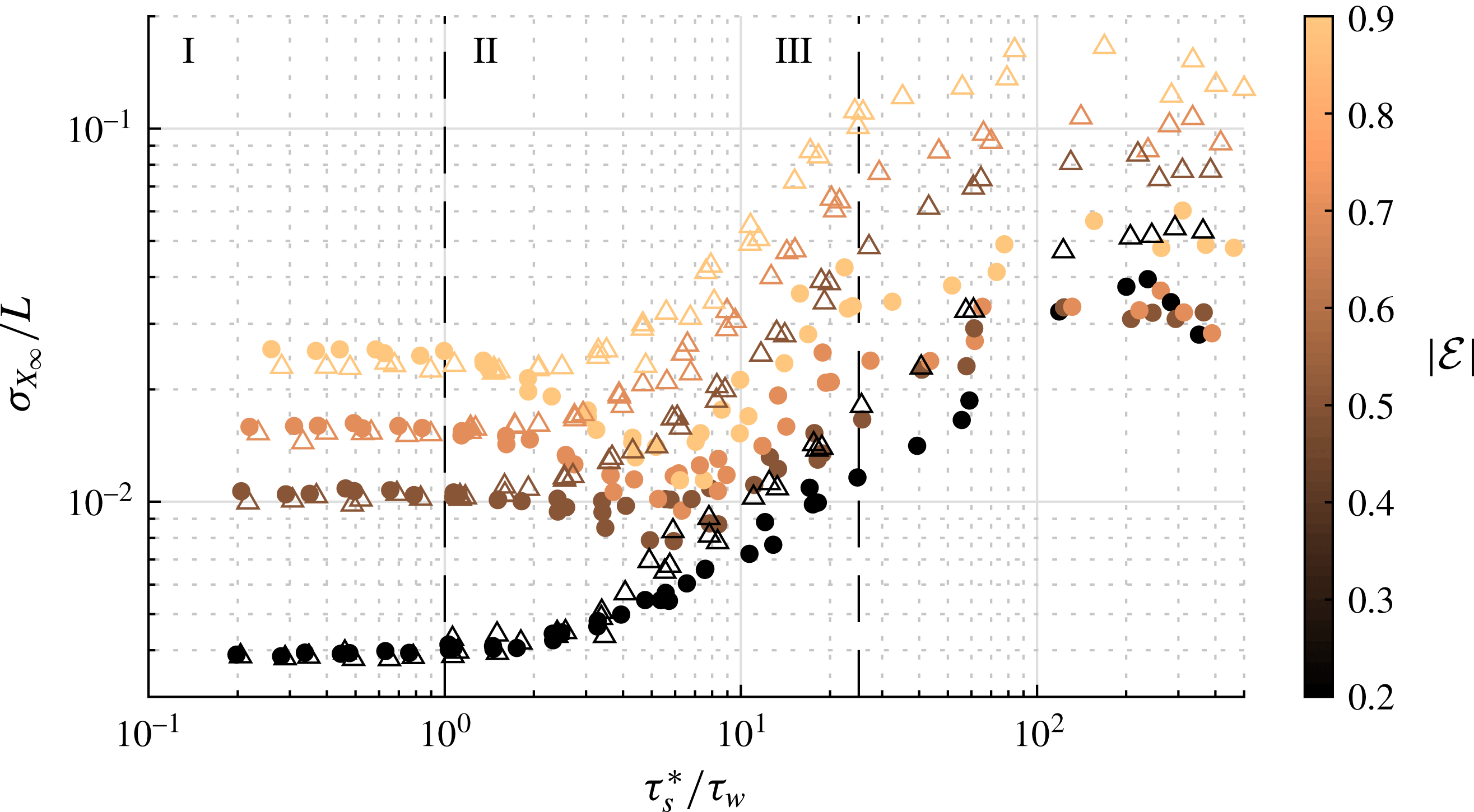
In the settling regime,
 $\unicode[STIX]{x1D70F}_{w}>\unicode[STIX]{x1D70F}_{s}^{\ast }$
. Here, the particles settle out of the wave field before they have a chance to be transported horizontally. They do not remain in the water column long enough for significant dispersion to take place, so whatever dispersion they do feel is due to various initial-condition-dependent lift forces on the particle as they sediment.
Once
 $\unicode[STIX]{x1D70F}_{w}$
and
 $\unicode[STIX]{x1D70F}_{s}^{\ast }$
are of the same order, the dispersion data deviate from the flat distributions seen in the settling regime and enters the dispersive regime. Here, the
 $\unicode[STIX]{x1D70E}_{x\infty }$
values of the oblate particle plumes increase monotonically with
 $\unicode[STIX]{x1D70F}_{s}^{\ast }/\unicode[STIX]{x1D70F}_{w}$
. This occurs because the particles are transported through the wave field for a longer distance before they settle out. If solely examining the oblate particle results, one would conclude that the larger
 $\unicode[STIX]{x1D70F}_{s}^{\ast }/\unicode[STIX]{x1D70F}_{w}$
ratios within this regime are indicative of more dispersion. However, for some of the prolate particles, the relationship is more complicated. For high-eccentricity prolate particles (
 ${\mathcal{E}}>0.2$
), dispersion in fact decreases at the onset of the dispersive regime. This is due to the fact that the particles are starting to align. The rate at which the particles align is not constant, as seen in figure 7; and in fact, the rate at which they align decreases over time. Therefore, the particles first quickly align to similar orientations, resulting in similar forcing on the particle and suppressing the dispersion. This bulk alignment rate is very different for oblate and prolate particles due to their different moments of inertia. Prolate particles are all almost aligned as they move through the dispersive regime, although some variability in their orientations still remains; thus, the dispersion is not removed but rather only slowed and is able to grow again at larger
 $\unicode[STIX]{x1D70F}_{s}^{\ast }/\unicode[STIX]{x1D70F}_{w}$
values. Oblate particles, on the other hand, have a much broader distribution of orientations, and their dispersion is stronger.
Finally, in the aligned regime, the particles have been in the waves long enough that they have all reached their preferred alignment. At this point, the dispersion ceases to grow, since the mechanism that drives it has been removed.
Our results demonstrate that the more anisotropic the particle, the more dispersion will be observed. But we also find that oblate ellipsoids disperse much more than their prolate counterparts. And, in general, more dispersion occurs when the transport is strong compared to the particle settling, or equivalently when the wave transport time scale is much shorter than the settling time scale. Furthermore, while there is a mechanism for dispersion in these simulations, we have demonstrated that the particles do not disperse without bound – in other words, if one were to predict that the anisotropic particles do not align and instead persist in random orientations, one would over-predict particle dispersion.
3.4 Effects of waviness
So far, our discussion has focused primarily on the properties of the Stokes drift rather than on the waves themselves. But the effect of the waves is not unimportant for the mean transport and dispersion of the particles. Here, we define the ‘waviness’ as the unsteady oscillating component of the flow. We isolate the effects of the waviness on transport by repeating the simulations using only the residual Stokes drift velocity field. This leads to a steady shear flow that decays exponentially with depth, described by (2.12). Note that this flow is no longer irrotational.
Orientation of identical prolate spheroids as a function of time in the same residual wave field with various initial orientations. The various colours represent corresponding orientation angles, for (a) polar angle
 $\unicode[STIX]{x1D719}$
and (b) azimuthal angle
 $\unicode[STIX]{x1D703}$
for particles started with different initial orientations in a deep-water residual Stokes drift velocity field as a function of time normalized by wave period. All particles have
 ${\mathcal{E}}=0.6$
and are inertialess. All oblate and prolate particles undergo similar orbits.

In a steady creeping shear flow, the particles undergo the expected Jeffery orbits. This is clearly seen when the particles from figure 5 were evolved in the deep-water residual Stokes drift velocity field alone. We show the corresponding orientation as a function of time in figure 12. Each particle undergoes a three-dimensional periodic orbit. The period is the same in all cases, as it is solely a function of the shear rate and aspect ratio. However, the type of orbit is dependent on initial orientation. The period of the orbits, as derived by Jeffery (Reference Jeffery1922), is
 $2\unicode[STIX]{x03C0}(\unicode[STIX]{x1D706}+1/\unicode[STIX]{x1D706})/\dot{\unicode[STIX]{x1D6FE}}$
where
 $\dot{\unicode[STIX]{x1D6FE}}$
is the shear rate.
When negatively buoyant particles are evolved in this type of flow, we can measure the new
 $X_{\infty }$
and
 $\unicode[STIX]{x1D70E}_{x\infty }$
values and compare to the corresponding wavy cases. We find that there is a measurable difference in both dispersion and mean transport of the particles. This makes sense, as we have already confirmed that orientational drag is important for transport; therefore, variations in particle orientation should affect the mean transport. In the presence of waves, the particle plumes tend to disperse more, but there is less mean transport. Particles in the Settling regime have identical plume dispersion with or without the wavy flow, but particles in the dispersive and aligned regime all have more dispersion in waves, with
 $\unicode[STIX]{x1D70E}_{x\infty }$
in some cases more than an order of magnitude higher. However, there is no clear trend indicating what controls this deviation. The mean transport is up to 30 % higher in the residual flow case. These results indicate that there remains much to be learned about the detailed effects of waves on particle transport.
4 Discussion and conclusions
To summarize our results, we conducted simulations of particle transport under linear surface gravity waves, extending previous work on this problem by incorporating the effects of particle anisotropy. We found that both prolate and oblate spheroids show preferred orientations, even without particle inertia. This alignment persists when the particles have weak inertia and must be considered when computing the particle’s mean settling velocity and transport. We also demonstrated that particle anisotropy causes the dispersion of particle plumes released with different initial orientations. Moreover, this dispersion cannot grow indefinitely as the particles will all eventually align if in the water column long enough. The unsteady shearing in waves both qualitatively and quantitatively affects how the particles are oriented and transported. Finally, our results suggest that the non-dimensional parameter that best describes the transport of weakly inertial anisotropic particles in wavy flows is not
 $St$
or
 $Re_{p}$
but rather the velocity ratio
 $u_{s}/w_{p}^{\ast }$
. This ratio captures the relative importance of the wave steepness
 $kA$
, which corresponds to the amount of shear in the flow, and
 $St$
, which captures the drag as the particle settles out of the wave field, as well as the preferred particle orientation.
Even though our simulations have revealed many features of the dynamics of spheroidal particles in wavy flows, there are many aspects that we have certainly not fully captured and that warrant further study. For example, we have assumed drag laws and torques that are only exact in the Stokes flow regime, where
 $Re_{p}\ll 1$
. The drag coefficients vary as
 $Re_{p}$
increases above unity, and as
 $Re_{p}$
grows past approximately 22, the laminar wakes of the particles may detach, and the drag should be re-parameterized (Zastawny et al.
Reference Zastawny, Mallouppas, Zhao and Van Wachem2012). Nevertheless, although the specifics of the drag coefficients will change in this intermediate
 $Re_{p}$
regime, the anisotropy of the drag forces, as well as the variation for different eccentricities, will remain (Ouchene et al.
Reference Ouchene, Khalij, Arcen and Tanière2016); and, as we have shown, the underlying physical mechanism for the effects we have observed is this anisotropic drag coupled with the dynamics of the flow field. The torques on the particle will be dependent on a rotational Reynolds number based on the particle’s length scale and angular velocity. Although the details of how Reynolds-number-dependent torques will affect our results are not clear at this time, the relationship between angle of attack and eccentricity will remain at increased Reynolds number (Ouchene et al.
Reference Ouchene, Khalij, Arcen and Tanière2016). Thus, although we would expect our results to change quantitatively with a different assumed drag law and torque parameterization, the same qualitative effects seen should still hold with increased particle inertia.
We have also shown that the specific nature of the flow field matters in determining the particle transport, since we find qualitatively different results when considering full wavy flows or only the residual shear component. We have not, however, studied the effects of turbulence, which may affect the preferred particle orientation we have observed. For example, there exists a limit when the effects of turbulence outweigh those of the waves, where the particles react as if they were subjected to turbulence alone. However, weaker turbulence will likely introduce a stochastic component to the particle motion while not necessarily destroying the preferential orientation. We leave these questions for more detailed numerical simulations or laboratory experiments.
Finally, while we have primarily considered negatively buoyant particles here, the same ideas apply to positively buoyant particles. However, since the shear rotating the particles is much weaker at depth in wavy flows, the quantitative results may be somewhat different. Furthermore, once the particles reach the surface, other forces may become important, affecting the long-term transport of positively buoyant particles in additional ways. We anticipate that this will be a fruitful area of study.
Acknowledgements
M.H.D. gratefully acknowledges the support of the Stanford Graduate Fellowship. This work was supported by the US National Science Foundation under grant no. CBET-1706586.



