Introduction
Estuaries provide many important ecological functions and services. Shallow estuaries with soft sediments provide ecological services that are predominately due to their extensive seagrass meadows. Seagrasses provide habitat, food, and shelter for diverse migratory and resident organisms, some of which have high commercial value. Seagrasses also improve sediment stability and prevent erosion (Orth et al., Reference Orth, Carruthers, Dennison, Duarte, Fourqurean, Heck, Hughes, Kendrick, Kenworthy, Olyarnik, Short, Waycott and Williams2006; Duarte et al., Reference Duarte, Kennedy, Marbà and Hendriks2013; Lavery et al., Reference Lavery, Mateo, Serrano and Rozaimi2013; Bartelli and Unsworth, Reference Bartelli and Unsworth2014; Dahl et al., Reference Dahl, Deyanova, Gütschow, Asplund, Lyimo, Karamfilov, Santos, Björk and Gullström2016; Brodie and N'Yeurt, Reference Brodie and N'Yeurt2018). Globally, seagrass meadows play important roles in nutrient production and cycling (Levin et al., Reference Levin, Boesch, Covich, Dahm, Erséus, Ewel, Kneib, Moldenke, Palmer, Snelgrove, Strayer and Weslawski2001), while their sediments also play an important role in carbon dioxide sequestration (Dahl et al., Reference Dahl, Deyanova, Gütschow, Asplund, Lyimo, Karamfilov, Santos, Björk and Gullström2016; Dahl et al., Reference Dahl, Asplund, Björk, Deyanova, Infantes, Isaeus, Nyström Sandman and Gullström2020; Shulkin et al., Reference Shulkin, Zharikov, Lebedev and Bazarov2024).
Seagrasses are sensitive to environmental conditions. Indeed, changes in environmental conditions are evident in tissue morphology, growth forms, distribution patterns, and growth rates (Fourqurean et al., Reference Fourqurean, Moore, Fry and Hollibaugh1997; Short and Duarte, Reference Short, Duarte, Shorts, Coles and Short2001). From the evidence to date, global warming is affecting the dynamics of seagrass beds. Short and Neckles (Reference Short and Neckles1999) summarized the effects of global climate change on seagrasses and concluded that the rise in global temperatures will alter seagrass growth rates, distributions, patterns of sexual reproduction, and other physiological functions. More recently, multiple studies have confirmed that rising sea surface temperatures (SSTs) affect seagrass ecosystems worldwide (Seddon et al., Reference Seddon, Connolly and Edyvane2000; Levin et al., Reference Levin, Boesch, Covich, Dahm, Erséus, Ewel, Kneib, Moldenke, Palmer, Snelgrove, Strayer and Weslawski2001; Gaeckle and Short, Reference Gaeckle and Short2002; Solana-Arellano et al., Reference Solana-Arellano, Echavarria-Heras and Leal-Ramirez2009; Marbá and Duarte, Reference Marbá and Duarte2010; Jordà et al., Reference Jordà, Marbà and Duarte2012; Brodie and N'Yaurt, Reference Brodie and N'Yeurt2018).
Some of these seagrass studies have examined the effects of rising sea levels due to high SST (Short and Neckles, Reference Short and Neckles1999; Duarte et al., Reference Duarte, Martins, Rosa, Matos, Roleda, Reush, Engleen, Serrao, Pearson, Marques, Cacador, Duarte and Jueterbock2018), while others have documented the loss of seagrass meadows, reporting that some have become functionally extinct (Höffle et al., Reference Höffle, Thomsen and Holmer2011; Jordà et al., Reference Jordà, Marbà and Duarte2012; Brodie and N'Yeurt, Reference Brodie and N'Yeurt2018). The loss of seagrass meadows inherently implies a loss of ecological services and habitats, which greatly affects the ability of seagrasses to sequester carbon. The consequences of these losses are global in scope. Orth et al. (Reference Orth, Carruthers, Dennison, Duarte, Fourqurean, Heck, Hughes, Kendrick, Kenworthy, Olyarnik, Short, Waycott and Williams2006) emphasized the urgency of prioritizing global conservation efforts for seagrass ecosystems, highlighting the crucial need for further research in seagrass meadows. Although the effects of climate change on seagrass meadows and habitats have been widely documented, the interactions between global warming and seagrass ecosystem dynamics require further study to develop sustainable management strategies for these crucial ecosystems.
Seagrasses exhibit clonal growth; meristematic activity results in the growth of rhizome nodules that form rhizome segments with bundles of attached shoots, leaves, and related roots (Tomlinson, Reference Tomlinson1974; Marbá and Duarte, Reference Marbá and Duarte1998; Vieira et al., Reference Vieira, López and Creed2018). In addition, seagrass biomass, density, and growth patterns are species-specific characteristics (Duarte, Reference Duarte1991; Duarte and Chiscano, Reference Duarte and Chiscano1999; Brun et al., Reference Brun, Vergara, Peralta, García-Sánchez, Hernández and Pérez-Lloréns2006; Vieira et al., Reference Vieira, López and Creed2018) that show strong seasonal and site dependence (Brun et al., Reference Brun, Vergara, Peralta, García-Sánchez, Hernández and Pérez-Lloréns2006; Turner, Reference Turner2007; Solana-Arellano et al., Reference Solana-Arellano, Echavarria-Heras and Leal-Ramirez2009; Solana-Arellano et al., Reference Solana-Arellano, Echavarria-Heras and Franco-Vizcaíno2010; Wong et al., Reference Wong, Bravo and Dowd2013; Vieira et al., Reference Vieira, López and Creed2018). Another of these characteristics is the plastochrone interval (PI), which is the time interval (days) between the formation of successive leaves (Jacobs, Reference Jacobs1979).
The PI concept was introduced by Erickson and Michelini (Reference Erickson and Michelini1957) in their study of Xanthium plants. Some years later, Jacobs (Reference Jacobs1979) used PI to evaluate the seagrass Zostera marina (Linnaeus, 1753). Since then, PI has been widely used in seagrass assessments and metabolic or physiological studies of leaf production (Dennison, Reference Dennison, Phillips and McRoy1990); growth, production, and biomass (Marbá et al., Reference Marbá, Cebrian, Enriquez and Duarte1996; Short and Duarte, Reference Short, Duarte, Shorts, Coles and Short2001; Gaeckle and Short, Reference Gaeckle and Short2002; Echavarria-Heras et al., Reference Echavarria-Heras, Solana-Arellano, Leal-Ramírez and Castillo2013); primary production (Erftemeijer and Herman, Reference Erftemeijer and Herman1994); and shoot age (Duarte and Sand-Jensen, Reference Duarte and Sand-Jensen1990; Duarte et al., Reference Duarte, Marbá, Agawin, Cebrián, Enriquez, Fortes, Gallegos, Merino, Olesen, Sand-Jensen, Uri and Vermaat1994; Tupan et al., Reference Tupan, Pentury and Uneputty2016; Fang et al., Reference Fang, Hang, Wang, Jiansheng and Li2018). Therefore, PI is an important and useful index in research on seagrass demography (e.g. Kraemer and Alberte, Reference Kraemer and Alberte1993; Van Tussenbroek, Reference Van Tussenbroek2002).
Every Z. marina leaf that is produced corresponds to a rhizome node that was formed leaving a scar in the rhizome; therefore, clonal growth and leaf formation can be considered equivalent processes in this seagrass (Jacobs, Reference Jacobs1979; Duarte et al., Reference Duarte, Hemminga and Marbá1996). Thus, it is reasonable to assume that variation in PI can be used to understand the architectural traits of Z. marina and the effects of environmental change (Brun et al., Reference Brun, Vergara, Peralta, García-Sánchez, Hernández and Pérez-Lloréns2006; Turner, Reference Turner2007). In particular, it is likely that the effects of climate change will be reflected in the seasonal patterns of PI variability.
This study aimed to (1) evaluate the tendency, seasonality, and interannual variability of the PI time series in a Z. marina meadow in Baja California using Bayesian statistics and (2) associate SST with changes in the PI time series.
Materials and methods
Study site
Data were collected in a Zostera marina meadow in the Punta Banda Estuary, located near Ensenada, Baja California, Mexico (31°44′N, 116°38′W). A Mediterranean climate characterizes the estuary, with warm summers (maximum temperature of 28°C) and cool humid winters (10°C) (Martinez-Inostros, Reference Martínez-Inostros1994). The salinity in the estuary ranges from 33.5 to 37.3‰ during winter (Acosta-Ruiz and Alvarez-Borrego, Reference Acosta-Ruiz and Alvarez-Borrego1974; Martinez-Inostros, Reference Martínez-Inostros1994). Normally, evaporation is greater than precipitation, but extreme winter storms can drive freshwater inputs that result in precipitation exceeding evaporation.
The Punta Banda Estuary has an approximate area of 18.71 km2. During the maximum high tide, ~16.40 km2 of the estuary is covered by water. The main channel (4–8 m depth) of the estuary covers ~1.78 km2. The estuary also contains mudflats that cover 2.85 km2, in which Z. marina is the only seagrass present. Zostera marina grows from the mudflats at a depth of −7 m (mean lower, low water) to the main channel (Flores-Uzeta, personal communication). Muddy banks are also present in the middle and at the head of the estuary. Seagrasses and green macroalgae grow on these banks, forming large mats that are clearly visible at low tide. Seagrasses and green algae have adapted to being periodically and completely covered by water (Pritchard et al., Reference Pritchard, de la Paz-Vela, Cabrera-Muro, Farreraz and Morales1978). The tides in the area are semidiurnal and play a notable role in the dynamics of the estuary. For example, up to 60% of the water in the estuary can ebb in one tidal cycle (Ibarra-Obando and Poumian-Tapia, Reference Ibarra-Obando and Poumian-Tapia1991).
Sampling, data processing, and statistical methods
During low tides, eelgrass was sampled using the Kentula and McIntire (Reference Kentula and McIntire1986) marking technique. The technique consists of marking the eelgrass shoots at the ligule (scar at the top of the sheath) by inserting a 22-gauge hypodermic needle through all the leaves just above the level of the youngest sheath. Marking and recovery depends on the tide. We sampled approximately every 2 weeks (13–17 days), the seagrass samples were collected. The complete data set is composed of the following periods: April 1998 to September 2003, October 2005 to March 2006, July 2008 to December 2013, September 2015 to April 2016, and November 2017 to August 2018. The data represent 316 biweekly sampling dates spanning approximately 158 months.
After marking the shoots, we recorded the number of leaves and placed a flag on the marked shoots (Meling-Lopez and Ibarra-Obando et al., Reference Meling-Lopez and Ibarra-Obando1997; Jimenez-Ramos et al., Reference Jiménez-Ramos, Henares, Egea, Vergara and Brun2023). During each sampling event, previously marked shoots were removed, and a new set of shoots were marked (40 during each sampling event). In laboratory, we recorded the number of new leaves, the leaf distance from the ligule to the needle mark (leaf growth), and number of leaves lost (number of leaves marked – number of leaves with needle marks). We also recorded the number of recovered shoots and the number of leaves. Following the methodology of Jacobs (Reference Jacobs1979), the average PI values associated with a sampling date t were calculated as follows:

where MS t is the number of recovered marked shoots at time t, $\nabla t$ is the time elapsed between sampling dates, and NLS t is the number of new leaves on marked shoots at time t.
A time series is a set of data recorded over time; it has its own components that act at the same time. The components of a time series are expressed by

where C t is the long-term trend; it is the pattern of the data over the time of analysis and constitutes the basis of an increase or reduction of the time series. S t characterizes data variation due to seasonal influences. I t is a set of cycles that last more than 1 year that can be due to a variety of factors. Finally, e t is the random error and explains the irregular and unpredictable behaviour of the time series (Brockwell and Davis, Reference Brockwell and Davis2002; Cowpertwait and Metcalfe, Reference Cowpertwait and Metcalfe2009; Shumway and Stoffer, Reference Shumway and Stoffer2010). In this study, we did not estimate I t due to a lack of data for some years in the PI t time series. Instead, we focus on C t and S t.
The tendency of the time series in terms of the response variable PI t was calculated fitting an equation of the form: C t = a + bt by the mean square method after removing seasonality by subtracting the PI mean of the log run series from each PI estimation (Cowpertwait and Metcalfe, Reference Cowpertwait and Metcalfe2009). A third degree polynomial was fitted to the PI data to show the decline on PI. Seasonality was assessed using the methodology of Grolemund and Wickham (Reference Grolemund and Wickham2011).
Water-column temperature and salinity were measured in situ with a digital thermometer and a portable refractometer (Leica, Wetzlar, Germany) respectively. To evaluate the degree of correlation between SST anomalies with monthly PI t means, we downloaded data from the Oceanic el Niño Index (ONI) (https://origin.cpc.ncep.noaa.gov/products/analysis_monitoring/ensostuff/ONI_v5.php). A one-way Bayesian analysis of variance (ANOVA) was used to identify differences in mean PI among years and seasons. All analyses were conducted in R (R Core Team, 2020).
Results
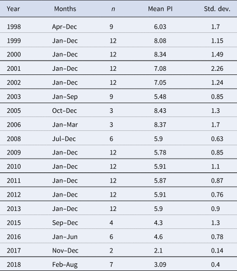
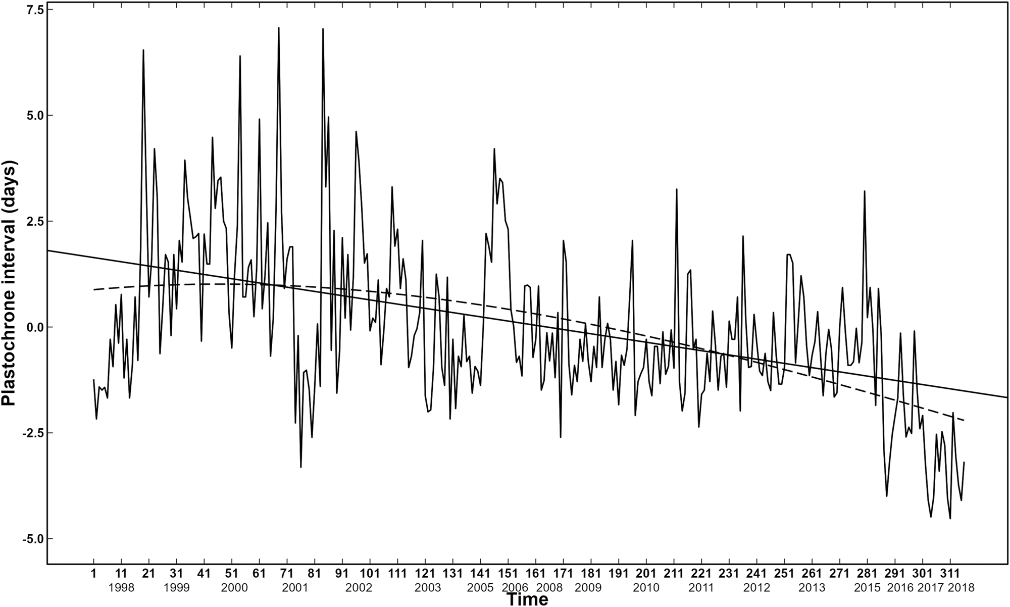
After fitting a Bayesian linear regression, the parameters of C t = a + bt of the time series were a = 1.65 ± 0.19 (95% credible intervals: [−1.27, 2.63]) and b = −0.01 ± 0.001 (95% credible intervals: [−0.012, −0.008]), and the Bayesian correlation coefficient was −0.495. The annual mean PI (days) values and standard deviation are shown in Table 1; the complete PI time series is shown in Figure 1.
Mean PI (days) and standard deviation per month

Complete biweekly PI means series measured in Punta Banda Estuary, Ensenada, México, without seasonality along with the Bayesian fitting tendency C t = a + bt with a negative b = −0 01 ± 0 001 with 95% credible intervals [−0. 02, −0 008].

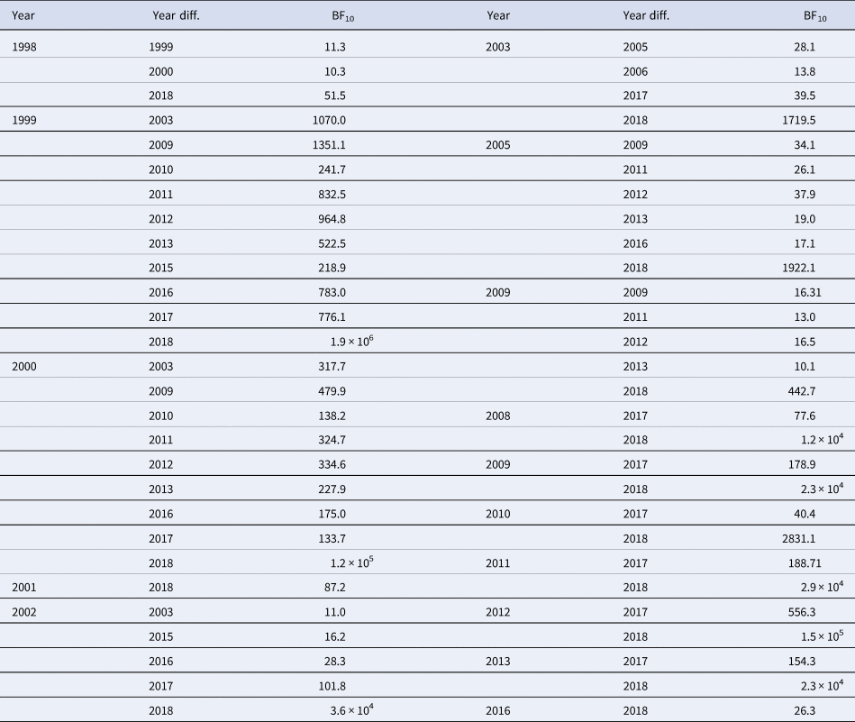
A Bayesian ANOVA showed strong evidence of differences among years with the Bayes factor (BF) ranging from 3.2 < BF < 1.88 × 10⁻⁶ (Table 2), indicating that the differences ranged from substantial to decisive (Jeffreys, Reference Jeffreys1935; Kass and Raftery, Reference Kass and Raftery1995). The biggest differences were found between hot and cold years. For example, 1999 exhibited cold SST anomalies, while 2010–2011 exhibited positive SST anomalies.
Bayesian ANOVA results

Second and fourth columns indicate the yearly differences with respect to year in first and third columns, whereas the third and sixth columns are the respective Bayes factors that indicate the probability of differences between years over the probability of equality between years. Individual comparisons are based on the default t-test with a Cauchy priori.
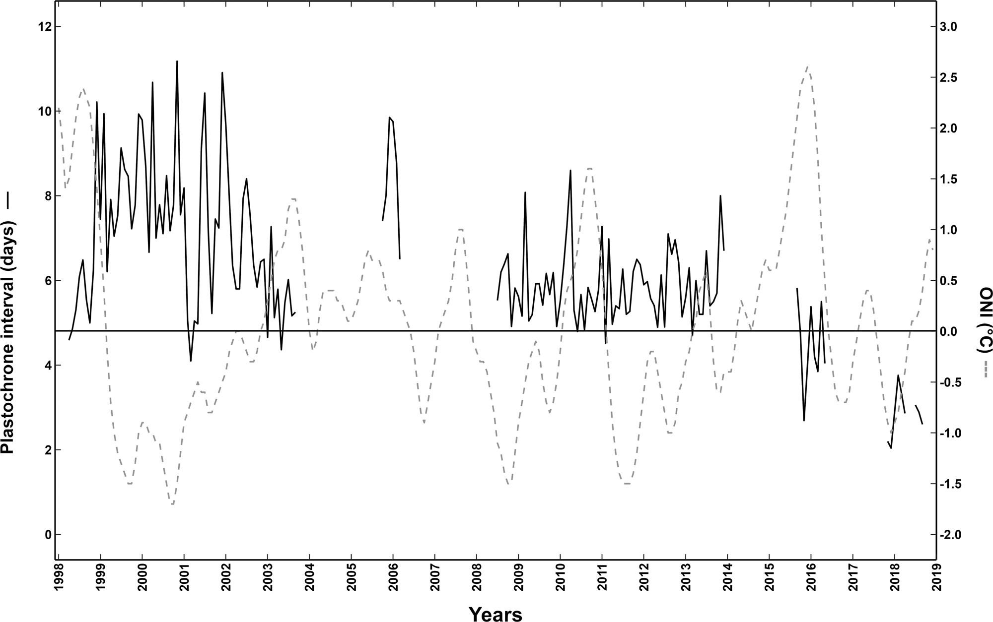
Monthly PI (days) means were calculated and correlated with the SST anomalies based on the monthly ONI. The estimated PI average for the whole series was 6.3 ± 1.9. Figure 2 shows the monthly PI series and SST anomalies. By 2018, the compound decedent tendency of PI resulted in PI declining three units below the overall mean. This could be the reason that most years exhibited a strong probability of being different from 2018 (Figure 2). Also, we found good correspondence between PI and ONI for most years (Figure 2). In particular, hot years that contained intermediate or strong El Niño events, such as 1997–1998, 2002–2003, 2010–2011, and 2015–2016, were associated with a decrease in PI values. Conversely, cold years, such as 1998–2002, 2008–2009, and 2012–2013, were associated with increasing PI values. Of note, a very long La Niña event occurred from 1998 to 2002, which decreased in strength over time.
Monthly PI average series (continuous line) and the corresponding ONI temperature anomalies (dashed line). Overall, there is a strong correspondence between PI and ONI in which positive anomalies are mostly associated with low PI values and negative anomalies correspond to high PI values.

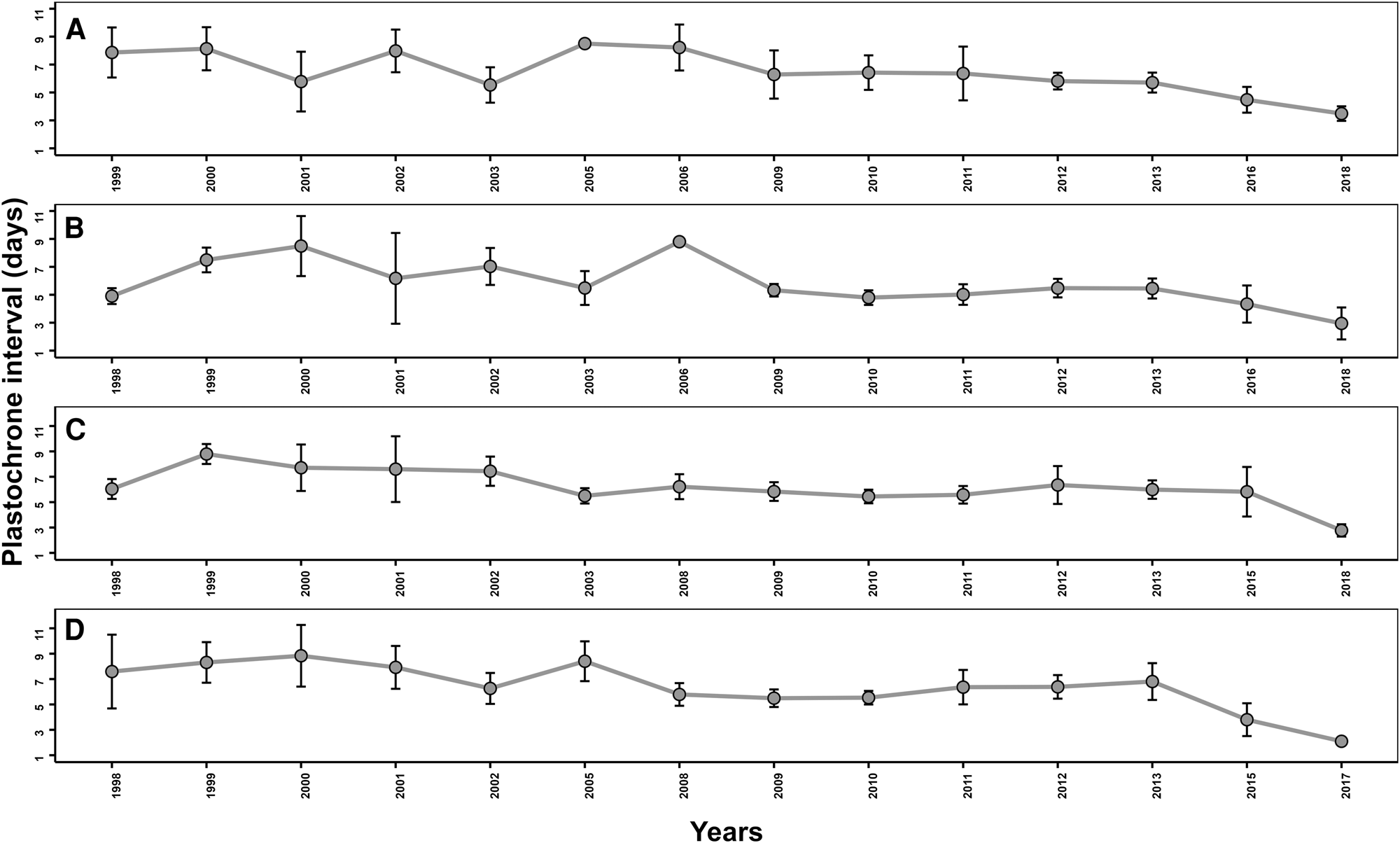
The PI series contained gaps because some months did not include sampling, the seasonal factor (equation (2)) could not be robustly estimated (Brockwell and Davis, Reference Brockwell and Davis2002). Nevertheless, we evaluated the climatology with the data, estimating the mean PI for the winter (December–February), spring (March–May), summer (June–August), and autumn (September–November) of each year (Figure 3). From the resulting climatology, we evaluated how PI varied during each season among different years (Figure 3), exhibiting a clear effect of seasonality on PI over time, since for all seasons, PI decline over time. Moreover, a Bayesian ANOVA was performed for each season's finding probability of differences (FB10 > 1.5) on PI among years; results are presented in the Supplementary material. Therefore, it is possible that climate change may be responsible for the variability observed in PI among years and seasons.
Seasonal representation of PI through years: (A) spring, (B) summer, (C) autumn, and (D) winter.

Discussion
Zostera marina is a dominant seagrass in temperate areas. It has been widely documented that temperature influences seagrass dynamics, especially those of Z. marina (Lee et al., Reference Lee, Park and Kim2007; Hosokawa et al., Reference Hosokawa, Nakamura and Kuwae2009; Solana-Arellano et al., Reference Solana-Arellano, Echavarria-Heras and Leal-Ramirez2009; Kaldy, Reference Kaldy2014; Kim et al., Reference Kim, Kim and Lee2015). Seasonality has also been found to affect seagrass dynamics, although this depends on the species and region (Ibarra-Obando et al., Reference Ibarra-Obando, Boudouresque and Roux1997; Azcárate-García et al., Reference Azcárate-García, Beca-Carretero, Cara, Villamayor, Cosnett, Bermejo, Hernández, Brun and Stengel2022; Salazar-Barrios, Reference Salazar-Barrios2015). Thus, we hypothesized that the rate of leaf and shoot formation (PI) varies seasonally. In normal consecutive years, we expected that seasonal PI fluctuations should be similar or that they should fluctuate around a stable average.
Overland et al. (Reference Overland, Rodionov, Minobe and Bond2008) suggested that these stable regimes can change gradually or abruptly due to perturbations or disturbances, such as increasing temperatures as in our study site. Azcárate-García et al. (Reference Azcárate-García, Beca-Carretero, Cara, Villamayor, Cosnett, Bermejo, Hernández, Brun and Stengel2022) evaluated seasonal vegetative development (morphology, population structure, and productivity) of Z. marina and Zostera noltii in western Ireland (cold temperatures) and southern Spain (warm temperatures) during 2017–2018 (Z. marina and Z. noltii) and 2019–2020 (only Z. noltii). The authors found that Z. marina in Ireland exhibited maximal growth during warmer months, while the Spanish population exhibited signs of growth reduction during periods of maximum annual temperatures, concluding that the optimal temperature for Z. marina in Spain was exceeded during summer, this could the case of our declining in PI. Moreover, Azcárate-García et al. (Reference Azcárate-García, Beca-Carretero, Cara, Villamayor, Cosnett, Bermejo, Hernández, Brun and Stengel2022) also demonstrated that leaf formation increased in Z. marina in Spain during autumn–winter 2017 and decreased during summer 2018 similarly as our results. Similarly, Johnson et al. (Reference Johnson, Shields, Kendrick and Orth2021) compared the survival of Z. marina in Chesapeake Bay (USA) after a warming event in 2005 and extraordinary precipitation and warming in 2018, reporting that these conditions led to large Z. marina declines. The authors concluded that (a) adult clone survival was lower in 2019 in regions with greater variation in temperature and salinity. (b) Mean bottom cover in recovering populations was higher in 2019 than 2006 despite lower adult survival due to high seedling abundance. (c) ‘If climate change increases the frequency of extreme events in the Chesapeake Bay and elsewhere, perennial Z. marina populations may be increasingly dependent on the previous years’ flowering and recruitment from seed’.
The mean annual PI showed an apparent decline over time and a clear agreement with SST anomalies (Table 1, Figure 2). It is therefore likely that temperature changes could have affected PI among years and seasons. Further, the mean annual PI ranged between 2.1 and 8.4 days, which is far below the ranges that have been reported in the literature for this species worldwide (13–28.7 days, Jacobs, Reference Jacobs1979; 9–14 days, Wium-Andersen and Borum, Reference Wium-Andersen and Borum1984; 8–18.86 days, Kentula and McIntire, Reference Kentula and McIntire1986; 10–30 days, Gaeckle and Short, Reference Gaeckle and Short2002). Moreover, our PI assessments generated a range of values that were lower than the ranges that have been reported for this species in the study region (6.4–12 days, Ibarra-Obando and Huerta-Tamayo, Reference Ibarra-Obando and Huerta-Tamayo1987; 5.7–11.2 days, Ibarra-Obando et al., Reference Ibarra-Obando, Boudouresque and Roux1997).
Seagrass plasticity, which is the capacity of seagrasses to acclimate to environmental stressors like increasing temperature (Hemminga and Duarte, Reference Hemminga and Duarte2000; McDonald et al., Reference McDonald, Prado, Heck, Forqurean, Frankovich, Dunton and Cebrian2016), may allow some seagrass species to withstand changing environmental conditions through morphological changes (Ruesink et al., Reference Ruesink, Fitzpatrick, Dumbauld, Hacker, Trimble, Wagner and Wisehart2012). In the Punta Banda Estuary, along with the declining PI, we observed an increase in the expansion of the meadow and number of leaves but a substantial decrease in the number of shoots and leaf length (Solana-Arellano and Flores-Uzeta, unpublished data). Moreover, we also observed an increase in opportunistic species, such as Gracilaria vermiculophylla (Salazar-Barrios, Reference Salazar-Barrios2015) and Ruppia maritima (Johnson et al., Reference Johnson, Williams, Lieberman and Solbak2003).
Shifts in PI dynamics may have negative effects on the ecology of seagrass ecosystems because elevated SSTs could induce multifarious responses in eelgrass metabolism (Hosokawa et al., Reference Hosokawa, Nakamura and Kuwae2009). Moreover, the relationship between the time series of PI and SST anomalies (ONI) (Figure 2) indicates that hot years were generally associated with low PI values. Johnson et al. (Reference Johnson, Williams, Lieberman and Solbak2003) directly linked the 1997–1998 El Niño with seagrass colonization in San Diego, California. The authors concluded that high SST, with anomalies ranging from 1.5 to 2.5°C, could be responsible for the observed shift in dominance from Z. marina to R. maritima, which likely caused changes in ecosystem functioning. Moreover, Thom et al. (Reference Thom, Southard and Borde2014) showed that SST and mean sea level were directly related to the ONI and closely related to eelgrass leaf growth and density in three estuaries in Washington state (USA). The authors concluded that seagrasses should be considered valuable indicators of the effects of climate change, specifically temperature variation in marine ecosystems, due to the close relationship between climate and seagrass dynamics. Furthermore, Jordá et al. (Reference Jordà, Marbà and Duarte2012) concluded that seagrass mortality was due to an increase in maximum annual SST and predicted the extinction of Posidonia oceanica in the Mediterranean Sea by 2049 if current warming conditions continue.
Given our findings of declining (or shifting) PI, if SST continues to rise due to global warming, Z. marina in the Punta Banda Estuary is likely to exhibit morphological changes with unknown ecological consequences for this important marine ecosystem. Further research is needed to understand how PI may change due to this stressor and the possible consequences of these changes for the ecosystem.
Supplementary material
The supplementary material for this article can be found at https://doi.org/10.1017/S0025315425000190
Data availability
Data are available on request from the authors.
Acknowledgements
We thank Andrea Lievana-MacTavish for the English revision of the manuscript.
Author contributions
E. S.-A. conducted the sampling over the entire time period, analysed and interpreted data, and wrote the manuscript. O. F.-U. conducted technical work, sampling, and sample processing during the entire period of time. C. E. C.-R., helped with the last 2 years of samplings and help with the data files. J. A. A.-C. contributed with data curation, analyses and the review/edition of the manuscript for the second peer-review.
Financial support
The is study was supported by Mexican Government.
Competing interests
None.