


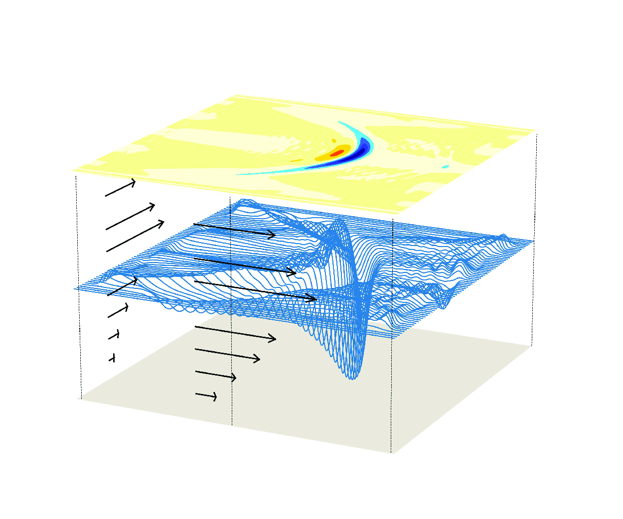



1. Introduction
Over the last few decades, internal waves in the ocean have gained significant attention due to advancements in our understanding of their substantial impact on oceanic energy cascade, climate systems, marine engineering, underwater navigation and ocean ecological systems, as reviewed by Helfrich & Melville (Reference Helfrich and Melville2006), Woodson (Reference Woodson2018), Boegman & Stastna (Reference Boegman and Stastna2019) and Whalen et al. (Reference Whalen, de Lavergne, Garabato, Klymak, MacKinnon and Sheen2020). This interest began with the pioneering work of Osborne & Burch (Reference Osborne and Burch1980), who utilised the Korteweg–de Vries (KdV) equation to analyse the observational internal solitary waves (ISWs) in the Andaman Sea. Theoretical equations have since become essential tools for exploring the dynamics of these waves and interpreting observational data. The KdV equation captures the interplay between nonlinear and dispersive effects, expressed mathematically as
 \begin{equation} A_t + c{\kern-1pt} A_x + \alpha A A_x + \beta{\kern-1pt} A_{xxx}=0, \end{equation}
where
 $A=A(x,t)$
is the wave amplitude,
 $c=c(x)$
denotes the linear wave phase speed, and
 $x$
and
 $t$
refer to the horizontal direction and time, respectively, with subscripts indicating partial derivatives. The nonlinear coefficient
 $\alpha =\alpha (x)$
and the dispersive coefficient
 $\beta =\beta (x)$
are determined by environmental factors such as variable topography, density stratification and background shear current (Grimshaw Reference Grimshaw1981, Reference Grimshaw1985; Yuan et al. Reference Yuan, Grimshaw and Johnson2018b
).
Inspired by these pioneering works, the KdV equation for oceanic ISWs has seen significant development and numerous variations. For example, Ostrovsky (Reference Ostrovsky1978) revisited the KdV equation to incorporate the effects of Earth’s rotation, resulting in the Ostrovsky equation; Grimshaw, Pelinovsky & Poloukhina (Reference Grimshaw, Pelinovsky and Poloukhina2002) derived a higher-order KdV equation that accounts for cubic nonlinear terms; Zhou & Grimshaw (Reference Zhou and Grimshaw1989) established a KdV-type model that includes the effects of variable background shear flow; Grimshaw (Reference Grimshaw1981, Reference Grimshaw1985) extended the equation from one horizontal dimension to two dimensions, resulting in the Kadomtsev–Petviashvili (KP) model. While some theoretical equations, such as the Miyata–Choi–Camassa equations (Miyata Reference Miyata1985, Reference Miyata1988; Choi & Camassa Reference Choi and Camassa1999), the Benjamin–Ono equation (Benjamin Reference Benjamin1966; Ono Reference Ono1975) and the modified Benney–Luke equation (Yuan, Wang & Chen Reference Yuan, Wang and Chen2020; Yuan & Wang Reference Yuan and Wang2022), demonstrate remarkable characteristics in specific scenarios, the KdV equation and its various adaptations remain the primary tools for interpreting observational data and understanding dynamics. This is largely due to its broad validity range, which often yields satisfactory results even under conditions beyond the formal assumptions (Ostrovsky & Stepanyants Reference Ostrovsky and Stepanyants2005).
Satellite observational data of (a) sea level anomaly (SLA) and (b) ISWs, in the South China Sea, on 23 April 2022. The data indicate that ISWs propagate into areas abundant with mesoscale eddies, marked by the blue and yellow patches in (a). This observation provides a paradigm for considering the effects of 2-D background shear currents on the evolution of ISWs. The red triangle marks where stratification is used for subsequent numerical computations. The SLA data were obtained from the AVISO website, https://www.aviso.altimetry.fr/en/data.html, while the satellite image was sourced from the NASA website, https://worldview.earthdata.nasa.gov.

Recent advancements in observational technology and numerical simulations have greatly improved our understanding of oceanic ISWs, particularly regarding their three-dimensional (3-D) spatial characteristics, where the effects of lateral spreading become significant (see figure 1; refer to Yuan & Wang Reference Yuan and Wang2022; Gong et al. Reference Gong, Li, Pawlowicz and Cai2023; Jia et al. Reference Jia, Gong, Zhang, Yuan and Zheng2024; Li & Sutherland Reference Li and Sutherland2024, amongst many others). However, most theoretical equations are constructed for a horizontally one-dimensional (1-D) framework, with only a few that can be generalised to examine 3-D variations (corresponding to the case of two horizontal dimensions). Among these, the KP equation is the most widely used, and its canonical form can be expressed as
 \begin{equation} \left ( A_t + c{\kern-1pt} A_x +\alpha A A_x + \beta{\kern-1pt} A_{xxx} \right )_x + \gamma{\kern-1pt} A_{yy} - \delta A = 0 , \end{equation}
where the additional terms, when compared to the KdV equation (1.1), indicate that
 $\gamma{\kern-1pt} A_{yy}$
represents the dispersive effects in the transverse
 $y$
-direction, and
 $\delta A$
signifies the long-wave dispersive effects induced by Earth’s rotation. Consequently, by utilising the vertical structures described by the modal function (Yuan et al. Reference Yuan, Grimshaw, Johnson and Chen2018c
), the 3-D fluctuations can be derived.
Indeed, Pierini (Reference Pierini1989) investigated the evolution of ISWs in the Alboran Sea under simplified conditions, specifically without considering varying environmental factors. His research was based on the regularised long-wave equation, closely resembling the KP equation with minor modifications. Later, Deng & Cai (Reference Deng and Cai2017) also employed the regularised long-wave equation to highlight the significance of Earth’s rotation on ISWs, particularly those with crestlines extending beyond
 $100$
km. Also, Cai & Xie (Reference Cai and Xie2010) and Yuan, Grimshaw & Johnson (Reference Yuan, Grimshaw, Johnson and Chen2018c
) utilised the KP equation to examine how islands and underwater canyons/plateaus influence the propagation of ISWs. Subsequently, Yuan et al. (Reference Yuan, Grimshaw, Johnson and Wang2018d
, Reference Yuan, Pan, Gao and Wang2023) applied the KP equation to explore the combined effects of variable topography and Earth’s rotation on the oblique interactions between two ISWs. However, these early studies focused primarily on one or two environmental factors. This limitation occurred partly because the classic KP equation (1.2) was sufficient at that stage for understanding the impact of individual factors. As research on ISWs has progressed, there is now a greater demand for a more in-depth understanding of internal wave dynamics when multiple factors are considered.
For instance, it has been known that the evolution of ISWs is significantly influenced by mesoscale eddies, as illustrated in figure 1. For example, Xie et al. (Reference Xie, He, Chen, Xu and Cai2015), Huang et al. (Reference Huang, Zhang, Zhang, Qian, Zhao and Tian2017, Reference Huang, Qiu, Zeng, Song, Guo and Chen2024) and Xu et al. (Reference Xu, He, Chen, Zhan, Wu, Xie, Shang, Ning, Fang and Cai2020) analysed observational data and numerical simulation results, revealing that the background shear currents induced by these eddies can reduce the variations of wave amplitudes by half. Nonetheless, the comparable spatial scales of the crest lengths of ISWs in the transverse direction and the radii of mesoscale eddies (as shown in figure 1) suggest that the effects of two-dimensional (2-D) background shear currents have to be considered in the propagation of ISWs. However, to the best of our knowledge, there are currently no reduced theoretical equations that account for 2-D background shear currents. To enhance our understanding of internal wave dynamics and aid in interpreting observational data, we propose a new theoretical equation. This equation retains the core characteristics of the classic KP equation while also incorporating the effects of 2-D background shear currents and Earth’s rotation.
The rest of the paper is structured as follows. In § 2, we derive a new theoretical equation that incorporates both 2-D background shear currents and Earth’s rotation by applying a multi-scale asymptotic expansion to simplify the rotational Euler equations. Given the complexity of analysing the proposed equation in its entirety, we first present a qualitative prediction in the same section. To examine the effects of each term in the equation, we design a corresponding numerical scheme that employs a pseudo-spectral method for spatial discretisation and a fourth-order Runge–Kutta method for time stepping, as described in § 3. The numerical results presented in § 4 highlight the significant impacts of both individual and combined effects of the 2-D background shear currents and Earth’s rotation, showcasing the potential effectiveness and applications of the proposed equation. Finally, in § 5, we offer concluding remarks and discuss the limitations of the newly developed model.
2. Mathematical formulations
2.1. Governing equations
We consider a 3-D inviscid and incompressible fluid characterised by continuous density stratification. A Cartesian coordinate system is established, where the
 $x$
-axis represents the direction of wave propagation, the
 $y$
-axis is the transverse direction, and the
 $z$
-axis indicates the vertical direction. According to convention, the
 $z$
-axis points upwards, with
 $z=0$
denoting the undisturbed free surface, and
 $z=-h_0$
representing the flat bottom at depth
 $h_0$
; see figure 2 for the schema. In the ocean, a typical scenario involves ISWs interacting with 2-D background shear currents, as mentioned in the Introduction. The ISWs have small wavelengths and high frequencies, even though the length of the wave crests in the transverse
 $y$
-direction is large, yet still smaller than the scale of the background currents. This observation likely justifies the assumption that horizontally uniform background currents – specifically, the flow components
 $u_0(z)$
in the
 $x$
-direction and
 $v_0(z)$
in the
 $y$
-direction – are adequate for examining the effects induced by 2-D background shear currents over a broad range.
Sketch of the problem and coordinate system.

We consider this configuration as the basic state, which consists of velocity components
 $u_0(z)$
and
 $v_0(z)$
in the respective
 $x$
- and
 $y$
-directions, along with the density distribution
 $\rho _0(z)$
and the pressure field
 $p_0(x,y,z)$
. When internal waves propagate into the region with this basic state, they introduce perturbed velocities
 $u(x,y,z,t)$
,
 $v(x,y,z,t)$
and
 $w(x,y,z,t)$
, as well as the perturbed density
 $\rho (x,y,z,t)$
and pressure
 $p(x,y,z,t)$
. The total velocity field can be expressed as
 $(u+u_0,v+v_0, w)$
, the total pressure field as
 $P=p_0+p$
, and the total density field as
 $\varrho =\rho _0+\rho$
. All these variables are governed by the rotational Euler equations, denoted as
 \begin{align} &\varrho [u_t+\left ( u+u_0\right )u_x+\left ( v+v_0 \right )u_y+w\left ( u+u_0\right )_z-f\left ( v+v_0 \right )] =-P_x + F_0^x,\end{align}
 \begin{align} &\varrho [v_t+\left ( u+u_0\right )v_x+\left ( v+v_0 \right )v_y+w\left ( v+v_0 \right )_z+f\left ( u+u_0\right )] =-P_y + F_0^y ,\end{align}
 \begin{align} \qquad w_t+\left ( u+u_0\right )w_x+\left ( v+v_0 \right )w_y+ww_z & = -\frac {P_z}{\varrho } -g ,\end{align}
 \begin{align} \qquad\varrho _t+\left ( u+u_0\right )\varrho _x+\left ( v+v_0 \right )\varrho _y+w\varrho _z & = 0 ,\end{align}
 \begin{align} \qquad u_x+v_y+w_z & = 0 ,\end{align}
where
 $f$
is the Coriolis parameter that accounts for the effects of Earth’s rotation,
 $F_0^x$
and
 $F_0^y$
denote the external forces in the
 $x$
- and
 $y$
-directions that drive the background shear currents, and the subscripts
 $x,y,z$
refer to differentiations with respect to the corresponding spatial dimensions. The boundary conditions at the respective free surface
 $z=\eta (x,y,t)$
and bottom
 $z=-h_0$
are
 \begin{eqnarray} &w=\eta _t+\left ( u+u_0\right )\eta _x+\left (v+v_0\right )\eta _y ,\quad P=P_a,\quad \text{at} \ z=\eta (x,y,t), \end{eqnarray}
 \begin{eqnarray} &w=0 \quad \text{at} \ z=-h_0, \end{eqnarray}
where
 $P_a$
denotes a constant atmospheric pressure. The vertical particle displacement of the fluid, represented as
 $\zeta (x,y,z,t)$
, is governed by
 \begin{equation} w=\frac {\mathrm{D}\zeta }{\mathrm{D} t}\; \Longrightarrow\; w=\zeta _t+\left (u+u_0\right )\zeta _x+\left (v+v_0\right )\zeta _y+w\zeta _z, \end{equation}
which satisfies the condition
 $\zeta =\eta$
at the free surface.
When internal waves cease – i.e. the perturbed velocity field has
 $u=v=w=0$
, and the perturbed density and pressure satisfy
 $\rho =p=0$
– (2.1)–(2.3) satisfy
 \begin{equation} f\rho _0v_0=p_{0x}-F_0^x \,,\quad f\rho _0 u_0 =-p_{0y}+F_0^y \,,\quad p_{0z}=-\rho _0 g , \end{equation}
while (2.4) and (2.5) hold automatically. It is noted that when there are no external forces, meaning
 $F_0^x=F_0^y=0$
, the basic state achieves a balance between rotation and pressure in the horizontal directions, while the hydrostatic balance is maintained in the vertical direction. This relationship can be used to simplify the primitive Euler system (2.1)–(2.5), resulting in the fully nonlinear perturbation equations for
 $(u,v,w,\rho ,p)$
:
 $\begin{eqnarray} \rm (\rho _0+\rho ) [ u_t+ ( u+u_0) u_x+ ( v+v_0 )u_y+w ( u+u_0 )_z-fv ] -\rho fv_0 +p_x=0, \end{eqnarray}$
 \begin{eqnarray} \rm (\rho _0+\rho ) [v_t+ ( u+u_0 ) v_x+ ( v+v_0)v_y+w ( v+v_0)_z+fu]+\rho fu_0 +p_y=0, \end{eqnarray}
 \begin{eqnarray} \rm(\rho _0+\rho )[w_t+ ( u+u_0) w_x+ ( v+v_0 )w_y+ww_z]+p_z+\rho g =0, \end{eqnarray}
 \begin{eqnarray} &\rho _t+ (u+u_0) \rho _x+ ( v+v_0) \rho _y+w\rho _z+w\rho _{0z}=0, \end{eqnarray}
 \begin{eqnarray} &u_x+v_y+w_z = 0, \end{eqnarray}
where the variables
 $(u_0,v_0,\rho _0,p_0)$
must satisfy (2.9).
2.2. Modelling
Following the classical KdV equation for internal waves (Grimshaw Reference Grimshaw1981, Reference Grimshaw1985), two small parameters,
 $\mu =h_0/\lambda \ll 1$
measuring dispersion and
 $\varepsilon =a/h_0\ll 1$
measuring nonlinearity, satisfy the relation
 $\varepsilon =\mathcal{O}(\mu ^2)$
, where
 $h_0$
is the water depth,
 $\lambda$
is a typical wavelength, and
 $a$
is a typical wave amplitude. We further assume that the fluid motion in the transverse
 $y$
-direction is of order
 $\mu$
slower than that in the primary-wave-propagating
 $x$
-direction. Under this assumption, the continuity equation (2.14) indicates that
 $v/u=w/u=\mathcal{O}(\mu )$
. To facilitate our derivation, we employ the multi-scale ansatz
 \begin{eqnarray} \rm u= \!\sum \limits _{j=1}^{\infty } \varepsilon ^j\,u_j (\theta ,Y,z,\tau ),\quad v=\mu \!\sum \limits _{j=1}^{\infty } \varepsilon ^j\,v_j (\theta ,Y,z,\tau ), \quad w=\mu \!\sum \limits _{j=1}^{\infty } \varepsilon ^j\,w_j (\theta ,Y,z,\tau ), \nonumber\\[7pt] \rm p=\sum \limits _{j=1}^{\infty } \varepsilon ^j\,p_j (\theta ,Y,z,\tau ),\quad \rho =\sum \limits _{j=1}^{\infty } \varepsilon ^j\,\rho _j (\theta ,Y,z,\tau ),\quad \zeta =\sum \limits _{j=1}^{\infty } \varepsilon ^j\,\zeta _j (\theta ,Y,z,\tau ), \nonumber\\ \hskip-2pc\end{eqnarray}
where
 $\theta =\mu (x-ct )$
,
 $Y=\mu ^2y$
and
 $\tau =\mu ^3t$
are slow variables, with the wave speed
 $c$
determined later in the analysis. Additionally, we assume that the effects of rotation and the particle velocity in the transverse
 $y$
-direction are small, with
 $f=\mathcal{O}(\varepsilon )$
and
 $v_0=\mathcal{O}(\mu )$
.
We substitute the above expansions into (2.10)–(2.14). Recalling that
 $\varepsilon =\mathcal{O}(\mu ^2)$
, we acquire, to leading order,
 \begin{eqnarray} &(c-u_0) \rho _0 \,u_{1\theta }-\rho _0 \,u_{0z}\, w_1-p_{1\theta }=0 , \end{eqnarray}
 \begin{eqnarray} &(c-u_0)\rho _0 \,v_{1\theta } - \rho _0 \, v _{0z} \,w_1 - p_{1Y} - f\left (\rho _0 u_1+\rho _1 u_0\right ) = 0, \end{eqnarray}
 \begin{eqnarray} &p_{1z}+g\rho _1=0, \end{eqnarray}
 \begin{eqnarray} &(c-u_0)\,\rho _{1\theta } - w_1\,\rho _{0z}=0, \end{eqnarray}
 \begin{eqnarray} &u_{1\theta }+w_{1z}=0, \end{eqnarray}
and (2.8) for the vertical particle displacement reduces to
 \begin{equation} w_1 + (c-u_0)\,\zeta _{1\theta } =0 . \end{equation}
To proceed with the derivation, the method of separation of variables is used by expressing the vertical displacement
 $\zeta _1 (\theta ,Y,z,\tau )$
induced by internal waves as the composition of wave amplitude
 $A (\theta ,Y,\tau )$
and vertical structure
 $\phi (z)$
, namely
 \begin{equation} \zeta _1=A (\theta ,Y,\tau )\,\phi (z). \end{equation}
Then substituting (2.22) into (2.21) and further into (2.16)–(2.20) leads to
 \begin{eqnarray} w_1 &=& -(c-u_0)\,A_\theta \,\phi,\quad u_1=A\left [(c-u_0)\,\phi \right ]_z,\quad \rho _1=-\rho _{0z}\,A\,\phi, \nonumber\\[6pt]&& p_1 =(c-u_0)^2\rho _0\,A\,\phi _z,\nonumber \\[6pt] v_{1\theta } &=& (c-u_0)\,A_Y\,\phi _z-A_\theta \,\phi \,v_{0z}+fA\sigma,\quad\sigma = \frac {\rho _0\left [(c-u_0)\,\phi \right ]_z-\rho _{0z}\,\phi \,u_0}{(c-u_0)\,\rho _0}, \nonumber\\\end{eqnarray}
and
 \begin{equation} [\rho _0\,(c-u_0)^2\,\phi _z]_z+\rho _0 N^2\phi =0, \end{equation}
where
 $N$
is the buoyancy frequency defined as
 $N=\sqrt {-({g}/{\rho _0}) ({\mathrm{d}\rho _0}/{\mathrm{d}z})}$
(also known as the Brunt–Väisälä frequency). In addition, the boundary conditions expressed in (2.6)–(2.7) show, to leading order, that
 \begin{align} (c-u_0)^2\phi _z=g\phi \quad &\mathrm{at}\ z=0, \end{align}
 \begin{align} \phi =0\quad &\mathrm{at}\ z=-h_0. \end{align}
Equations (2.24)–(2.26) form an eigenvalue problem that has an infinite number of solution pairs
 $(\phi _n,c_n)$
for
 $n=1,2,3,\ldots$
, where
 $n=1$
corresponds to the solution for long surface waves, and
 $n\geqslant 2$
represents the mode for
 $(n-1)$
. In particular, when the rigid-lid approximation is applied instead of the free surface condition, it leads to
 $\phi =0$
at
 $z=0$
, which excludes potential surface waves. In practice, once the specific mode
 $n$
is identified, the phase speed
 $c$
and the vertical structure
 $\phi$
can be determined uniquely using (2.24)–(2.26).
Expanding the governing system (2.10)–(2.14) to the next order yields
 \begin{align} & \rho _0[(c-u_0)\,u_{2\theta }-u_{0z}w_2]-p_{2\theta }\nonumber \\[6pt] & {}=\rho _0 (u_{1\tau }+u_1u_{1\theta }+w_1u_{1z} )+\rho _0v_{0}u_{1Y}-\rho _1[(c-u_0) u_{1\theta }-u_{0z}w_1]-f (\rho _0v_1+\rho _1v_{0} ), \end{align}
 \begin{align} & \rho _0[(c-u_0)v_{2\theta }-v_{0z}w_2]-p_{2Y}-f (\rho _0u_2+\rho _2u_0 )\nonumber \\[6pt] & {}=\rho _0 (v_{1\tau }+u_1v_{1\theta }+w_1v_{1z})-\rho _1 [(c-u_0)v_{1\theta }-{v}_{0z}w_1 ]+f\rho _1u_1+\rho _0{v}_{0}v_{1Y}, \end{align}
 \begin{equation} p_{2z}+g\rho _2=(c-u_0)\rho _0\,w_{1\theta }, \end{equation}
 \begin{equation} (c-u_0)\rho _{2\theta }-\rho _{0z}w_2=\rho _{1\tau }+u_1\rho _{1\theta }+w_1\rho _{1z}+v_0\rho _{1Y}, \end{equation}
 \begin{equation} u_{2\theta }+w_{2z}=-v_{1Y}. \end{equation}
Note that all terms on the right-hand side are known regarding the variables at the leading order. To address this problem, boundary conditions are required; however, upon examining (2.6)–(2.7), we find that the surface fluctuation
 $\eta$
must be considered at this stage. Thus to proceed, we expand
 $\eta$
as
 $\eta =\sum _{j=1}^{n}\varepsilon ^j\,\eta _j (\theta ,Y,\tau )$
. Recalling that at the surface
 $\zeta (\theta ,Y,z=\eta ,\tau )=\eta$
, the expansion at order
 $\mathcal{O}(\epsilon )$
leads to
 \begin{equation} \eta _1(\theta ,Y,\tau )=\zeta _1(\theta ,Y,z=0,\tau )=A\left (\theta ,Y,\tau \right )\,\phi \left (0\right )\! . \end{equation}
The expansion of
 $\eta$
allows us to establish the boundary conditions for (2.27)–(2.31) as follows:
 \begin{align} w_2+(c-u_0)\eta _{2\theta }=\eta _{1\tau }+u_1\eta _{1\theta }+u_{0z}\eta _1\eta _{1\theta }-w_{1z}\eta _1+v_0\eta _{1Y}\quad &\mathrm{at}\ z=0, \end{align}
 \begin{align} \eta _2-\zeta _2=\eta _1\zeta _{1z}\quad &\mathrm{at}\ z=0, \end{align}
 \begin{align} p_2-g\rho _0\eta _2=\frac {g\rho _{0z}}{2}\eta _{1}^{2}-\eta _1p_{1z}\quad &\mathrm{at}\ z=0, \end{align}
 \begin{align} w_2=0\quad &\mathrm{at}\ z=-h_0. \end{align}
The condition (2.34) is derived from the Taylor series of
 $\zeta (\theta ,Y,z=\eta ,\tau )=\eta$
at
 $z=0$
. Similarly, (2.8) at second order gives
 \begin{equation} w_2=-(c-u_0)\zeta _{2\theta }+A_\tau \phi -u_{0z}AA_\theta \phi ^2+v_0A_Y\phi . \end{equation}
Then substituting (2.37) into the incompressibility condition (2.30) and the continuity equation (2.31) yields, respectively,
 \begin{equation} \rho _2=\frac {\rho _{0zz}}{2}A^2\phi ^2-\rho _{0z}\zeta _2, \end{equation}
 \begin{equation} u_{2\theta }=(c-u_0)\zeta _{2\theta z}-u_{0z}\zeta _{2\theta }-A_\tau \phi _z+AA_\theta (u_{0z}\phi ^2)_z-({v}_{0}\phi)_zA_Y-v_{1Y}. \end{equation}
Solving for
 $p_{2\theta }$
using (2.27), (2.37) and (2.39), one obtains
 \begin{align} p_{2\theta }={}&\rho _0 (c-u_0)^2\zeta _{2\theta z}-\rho _0 (c-u_0) v_{1Y}-2\rho _0 (c-u_0) A_\tau \phi _z\nonumber \\[8pt] &{}+2\rho _0 (c-u_0) u_{0z}AA_\theta \phi \phi _z-2\rho _0 (c-u_0) v_{0}\phi _zA_Y-\rho _0 (c-u_0) v_{0z}\phi A_Y\nonumber \\[8pt] &{}+f\rho _0 v_1-f\rho _{0z}A\phi v_{0}-(c-u_0)^2AA_\theta (\rho _{0z}\phi \phi _z+\rho _0\phi _{z}^{2}-\rho _0\phi \phi _{zz}). \end{align}
By taking the derivative of (2.29) with respect to
 $\theta$
and then substituting (2.40) and (2.38) into the resultant equation, we arrive at
 \begin{align} & [\rho _0 (c-u_0)^2\zeta _{2\theta z}]_z-g\rho _{0z}\zeta _{2\theta }\nonumber \\[8pt] &=-(c-u_0)^2\rho _0A_{\theta \theta \theta }\phi +[\rho _0 (c-u_0) v_{1Y}]_z-g\rho _{0zz}AA_\theta \phi ^2\nonumber \\[8pt] &\quad{}+2A_Y[\rho _0 (c-u_0) v_{0}\phi _z]_z+A_Y[\rho _0 (c-u_0) {v}_{0z}\phi ]_z -f(\rho _0v_1)_z\nonumber \\[8pt] &\quad{}+AA_\theta [(c-u_0)^2(\rho _{0z}\phi \phi _z+\rho _0\phi _{z}^{2}-\rho _0\phi \phi _{zz})]_z+fA (\rho _{0z}\phi v_{0})_z\nonumber \\[8pt] &\quad{}-2AA_\theta [\rho _0 (c-u_0) u_{0z}\phi \phi _z ]_z +2A_\tau [\rho _0 (c-u_0) \phi _z ]_z. \end{align}
We next address the boundary conditions. Note that condition (2.36) implies
 $\zeta _{2\theta }=0$
at
 $z=-h_0$
, while condition (2.34) gives
 $\eta _2= \zeta _2+A^2\phi \phi _z$
at
 $z=0$
; thus (2.33) is satisfied automatically. Finally, the boundary condition (2.35) at
 $z=0$
can be recast to
 \begin{align} &\rho _0 (c-u_0)^2\zeta _{2\theta z}-g\rho _0\zeta _{2\theta }\nonumber \\[8pt] &=\rho _0 (c-u_0) A_Y{v}_{0z}\phi +\rho _0 (c-u_0) v_{1Y}+2\rho _0 (c-u_0) A_\tau \phi _z+2\rho _0 (c-u_0) A_Y v_{0}\phi _z\nonumber \\[8pt] &\quad{}+(c-u_0)^2AA_\theta (3\rho _0\phi _{z}^{2}-2\rho _0\phi \phi _{zz})-f\rho _0v_1+f\rho _{0z}A\phi {v}_{0}. \end{align}
Multiplying (2.41) by
 $\phi$
, and integrating with respect to
 $z$
from
 $z=-h_0$
to
 $z=0$
, gives the solvability condition:
 \begin{equation} \int _{-h_0}^{0} \{[\rho _0(c-u_0)^2\zeta _{2\theta z}]_z\phi -g\rho _{0z}\zeta _{2\theta }\phi \}\mathrm{d}z= [(c-u_0)^2\rho _0\zeta _{2\theta z}\phi -g\rho _{0}\zeta _{2\theta }\phi ]_{z=0}. \end{equation}
Finally, we substitute (2.41) and boundary condition (2.42) into (2.43). Using integration by parts, we obtain
 \begin{equation} \left ( A_\tau +\alpha A A_\theta + \beta{\kern-1pt} A_{\theta \theta \theta }+\chi A_Y+\iota A\right )_\theta +\gamma{\kern-1pt} A_{YY}-\kappa A_Y-\delta A = 0, \end{equation}
with the coefficients
 \begin{align} \alpha &= \displaystyle\frac {3\int _{-h_0}^{0}\rho _0 (c-u_0)^{2}\phi _{z}^{3}\mathrm{d}z}{2\int _{-h_0}^{0}\rho _0 (c-u_0) \phi _{z}^{2}\mathrm{d}z}\,, \quad \beta =\displaystyle\frac {\int _{-h_0}^{0}\rho _0 (c-u_0)^{2} \phi ^{2}\mathrm{d}z}{2\int _{-h_0}^{0}\rho _0 (c-u_0) \phi _{z}^{2}\mathrm{d}z}\,, \nonumber \\[8pt] \chi &=\displaystyle\frac {\int _{-h_0}^{0}\rho _0 (c-u_0) \phi _{z}^{2} v_{0}\mathrm{d}z}{\int _{-h_0}^{0}\rho _0 (c-u_0) \phi _{z}^{2}\mathrm{d}z}\,,\nonumber \\[8pt] \iota &= \displaystyle\frac {f\int _{-h_0}^{0}(\rho _0 v_{0})_z\phi \phi _{z} \mathrm{d}z}{2\int _{-h_0}^{0}\rho _0 (c-u_0) \phi _{z}^{2}\mathrm{d}z}\,, \quad \gamma =\displaystyle\frac {\int _{-h_0}^{0}\rho _0 (c-u_0)^{2}\phi _{z}^{2}\mathrm{d}z}{2\int _{-h_0}^{0}\rho _0 (c-u_0) \phi _{z}^{2}\mathrm{d}z}\,, \nonumber \\[8pt] \kappa &=\displaystyle\frac {f\int _{-h_0}^{0}(\rho _0u_0)_z\phi \phi _{z} \mathrm{d}z}{2\int _{-h_0}^{0}\rho _0 (c-u_0) \phi _{z}^{2}\mathrm{d}z}\,,\\[8pt] \delta &= \displaystyle\frac {f^2\int _{-h_0}^{0}\rho _0 \phi _{z}\sigma \mathrm{d}z}{2\int _{-h_0}^{0}\rho _0 (c-u_0) \phi _{z}^{2}\mathrm{d}z},\quad \text{with}\quad\sigma = \displaystyle\frac {\rho _0\left [(c-u_0)\,\phi \right ]_z-\rho _{0z}\phi u_0}{(c-u_0)\,\rho _0} \,. \nonumber \end{align}
Note that the proposed (2.44) takes into account the effects of both Earth’s rotation and 2-D background shear currents
 $(u_0,v_0)$
. If these factors are absent, meaning that
 $u_0=v_0=0$
and
 $f=0$
, then
 $\chi =\iota =\kappa =\delta =0$
. In this case, the equation simplifies to the classic KP equation; thus (2.44) will be referred to as the ‘KP-fusion’ equation hereafter, emphasising the evolution of internal waves under the influence of multiple coupling factors.
Notably, the KP-fusion equation (2.44) is not merely a nonlinear dispersive wave equation. The term
 $\iota A$
appears to be a manifestation of the Coriolis force in the
 $x$
-direction,
 $fv_0$
, and this extra force explains why the term can amplify or destroy waves as they propagate in the
 $x$
-direction and also why, if the term is of the correct sign and uniform in
 $x$
, it will cause solutions to grow arbitrarily large. Similarly, the term
 $\chi A_Y$
indicates a wave solution that propagates in the
 $Y$
-direction with speed
 $\chi$
. Nonetheless, the effects of the term
 $\kappa A_Y$
are more complex. In general, it signifies the decrease (when
 $l/k\lt 0$
) or increase (when
 $l/k\gt 0$
) of the Fourier components at modes
 $k$
and
 $l$
. Consequently, the overall variation of amplitudes cannot be determined easily, and requires numerical solutions for specific cases.
Given the water depth
 $h_0$
and the density profile
 $\rho _0(z)$
, the coefficient
 $\iota$
depends on the vertical structure of the background shear current
 $v_0$
in the
 $Y$
-direction, as well as the strength of Earth’s rotation
 $f$
, with
 $\iota =0$
in the case of either
 $v_0=0$
or
 $f=0$
. Similarly, the coefficient
 $\kappa$
depends on the vertical structure of the background shear current
 $u_0$
and the strength of Earth’s rotation
 $f$
, with
 $\kappa =0$
in the case of either
 $\partial _z u_0=0$
or
 $f=0$
. The wave propagation speed
 $\chi$
in the
 $Y$
-direction is determined by the background shear current
 $v_0$
. This consistent variation in amplitude, induced by
 $\iota A$
and
 $\kappa A_Y$
, suggests intricate energy transfer between the waves and the background currents. This phenomenon is partly due to the assumption that internal waves have smaller spatial scales compared to those of the background shear.
3. Numerical method
The KP-fusion equation (2.44) generally poses challenges in obtaining analytical solutions, which leads us to rely on numerical simulations. However, the terms associated with the Coriolis parameter
 $f$
usually require a long time to produce perceptible effects. To reduce computation time and enhance numerical efficiency, we introduce a scaling
 \begin{equation} A=\Upsilon \bar {A}\,,\quad \theta =L\bar {\theta }\,, \quad Y = L \bar {Y}\,, \quad \tau = L^3\bar {\tau }. \end{equation}
This scaling (3.1) effectively transforms the KP-fusion equation (2.44) into
 \begin{equation} \left ( \bar {A}_{\bar {\tau }} + \bar {\alpha } \bar {A} \bar {A}_{\bar {\theta }} + \bar {\beta } \bar {A}_{\bar {\theta }\bar {\theta }\bar {\theta }}+\bar {\chi } \bar {A}_{\bar {Y}} + \bar {\iota } \bar {A}\right )_{\bar {\theta }} + \bar {\gamma } \bar {A}_{\bar {Y}\bar {Y}}-\bar {\kappa } \bar {A}_{\bar {Y}}-\bar {\delta } \bar {A} = 0 , \end{equation}
where
 \begin{equation} \!\!\bar {\alpha }=\Upsilon L^2 \alpha \,,\quad \bar {\beta } = \beta \,, \quad \bar {\chi } = L^2 \chi \,, \quad \bar {\iota }=L^3 \iota \,, \quad \bar {\gamma } = L^2 \gamma \,, \quad \bar {\kappa } = L^3 \kappa \,, \quad \bar {\delta } = L^4 \delta . \end{equation}
Although the parameters
 $\Upsilon$
and
 $L$
can be chosen freely, in practice, scaling to ensure that the new nonlinear coefficient
 $\bar {\alpha }$
and the rotational coefficient
 $\bar {\gamma }$
are of order unity yields favourable results.
To accurately solve the scaled KP-fusion equation (3.2), we utilise a pseudo-spectral method based on the Fourier interpolant in the spatial domain while employing the fourth-order Runge–Kutta method for time stepping. By taking the 2-D Fourier transform, where
 $k$
and
 $l$
represent the Fourier modes in the respective
 $\theta$
- and
 $Y$
-directions, (3.2) can be expressed as
 \begin{equation} \hat {A}_{\bar {\tau }} =-\frac {\mathrm{i}k}{2} \bar {\alpha } \widehat {A^2} +\left ( \mathrm{i}k^{3}\bar {\beta }-\mathrm{i}l\bar {\chi } -\bar {\iota }-\frac {\mathrm{i}l^{2} }{k} \bar {\gamma } + \frac {l}{k}\bar {\kappa } -\frac {\mathrm{i}}{k}\bar {\delta } \right ) \hat {A}, \end{equation}
where
 $\mathrm{i}=\sqrt {-1}$
denotes the imaginary unit, and a hat indicates the Fourier coefficient, e.g.
 $\hat {A}=\mathcal{F} [\bar {A} ]$
, with
 $\mathcal{F}$
signifying the Fourier transform operator. To promote the stability and efficiency of the numerical scheme, we define
 \begin{equation} W=\mathrm{i}k^{3}\bar {\beta }-\mathrm{i}l\bar {\chi } -\bar {\iota }-\frac {\mathrm{i}l^{2} }{k} \bar {\gamma } + \frac {l}{k}\bar {\kappa } -\frac {\mathrm{i}}{k}\bar {\delta } . \end{equation}
Next, we multiply (3.4) by
 $\textrm{e}^{-W\bar {\tau }}$
and define
 $\widehat {U}=\textrm{e}^{-W\bar {\tau }}\hat {A}$
, transforming (3.4) into
 \begin{equation} \widehat {U}_{\bar {\tau }}=-\frac {\mathrm{i}k}{2} \bar {\alpha }\, \textrm{e}^{-W\bar {\tau }}\,\widehat {A^2} , \end{equation}
which can be practically rewritten as
 \begin{equation} \widehat {U}_{\bar {\tau }}+\frac {\mathrm{i}k}{2}\bar {\alpha }\, \textrm{e}^{-W\bar {\tau }}\,\mathcal{F}\left \{\left [\mathcal{F}^{-1} \left (e^{W\bar {\tau }}\,\widehat {U}\right ) \right ]^2 \right \} = 0 . \end{equation}
Nevertheless, in practice, the numerical algorithm encounters issues when dealing with terms where the first Fourier mode,
 $k=0$
, appears in the denominator. One possible solution is to simply set
 $\widehat {U}(k=0)=0$
at every time step. This indicates that
 $\int _\theta A\, \mathrm{d} \theta = 0$
, meaning that the integration of initial wave amplitude along the
 $\theta$
-direction must equal zero. This can be achieved by applying a reverse pedestal
 $A_p$
to the initial waves
 $A$
:
 \begin{equation} A_{ic} = A - A_p \quad \text{and}\quad A_p = A_s \left [\tanh \left (\frac {\theta +\theta _e}{\theta _w}\right ) - \tanh \left (\frac {\theta -\theta _e}{\theta _w}\right )\right ], \end{equation}
with
 $\int A\, \mathrm{d}\theta = \int A_p\, \mathrm{d}\theta$
. According to Yuan et al. (Reference Yuan, Grimshaw and Johnson2018a
), the length and slope of the pedestal are determined by the parameters
 $\theta _e$
and
 $\theta _w$
, which help to suppress the end effects of the pedestal. For this,
 $\theta _e=L^\theta /4$
and
 $\theta _w = L^\theta /8$
, with
 $L^\theta$
representing the length of the
 $\theta$
domain.
To reduce numerical noise and stabilise the simulations, an exponential filter
 $\varkappa$
is invoked to dampen the high-wavenumber components by filtering the Fourier field
 $\widehat {U} \to \varkappa \widehat {U}$
in both the
 $\theta$
- and
 $Y$
-directions (Subich, Lamb & Stastna Reference Subich, Lamb and Stastna2013). Following Subich et al. (Reference Subich, Lamb and Stastna2013) and Li & Sutherland (Reference Li and Sutherland2024), the filter is selected as
 \begin{equation} \varkappa (n) = \left \{ \begin{array}{lr} 1\,, & n\lt n_{{cut}}\,,\\[8pt] \exp \left [-e_1\left (\displaystyle\frac {n-n_{{cut}}}{n_m - n_{{cut}}}\right )^{e_2}\right ]\,, & n \geqslant n_{{cut}} , \end{array} \right . \end{equation}
where
 $n=n_\theta$
or
 $n_Y$
, indicating the number of Fourier modes in the respective
 $\theta$
- and
 $Y$
-directions. Here,
 $n_m=n/2$
,
 $e_1$
refers to the filter strength, and
 $e_2$
is the filter order. To effectively diminish numerical noise without affecting the wavenumber components that have non-negligible amplitudes, the cut-off parameters are set to
 $n_{{cut}}=0.6\, n_m$
,
 $e_1=20$
and
 $e_2=2$
, as suggested by Subich et al. (Reference Subich, Lamb and Stastna2013) and Li & Sutherland (Reference Li and Sutherland2024).
To address the rapid propagation of dispersive waves in the
 $Y$
-direction and the long waves induced by Earth’s rotation in the
 $\theta$
-direction, we introduce artificial boundary layers governed by coefficients
 $\varpi \lt 0$
. These layers are added to the right-hand side of (3.2), which results in
 \begin{equation} \left ( \bar {A}_{\bar {\tau }} + \bar {\alpha } \bar {A} \bar {A}_{\bar {\theta }} + \bar {\beta } \bar {A}_{\bar {\theta }\bar {\theta }\bar {\theta }}+\bar {\chi } \bar {A}_{\bar {Y}} + \bar {\iota } \bar {A}\right )_{\bar {\theta }} + \bar {\gamma } \bar {A}_{\bar {Y}\bar {Y}}-\bar {\kappa } \bar {A}_{\bar {Y}}-\bar {\delta } \bar {A} = \varpi \bar {A} . \end{equation}
In the inner domain, the coefficient
 $\varpi =\varpi (\theta ,Y)$
is zero and increases according to hyperbolic tangent functions, reaching specific values at the four boundaries.
(a) The summer density profile extracted from the World Ocean Atlas dataset 2018 at
 $20.5^{\,\circ}$
N,
 $118.5^{\,\circ}$
E, with an associated buoyancy frequency
 $N=\sqrt {-({g}/{\rho _0})({\mathrm{d} \rho _{0}}/{\mathrm{d} z})}$
. The specific location is illustrated in figure 1. (b) The vertical structures of the considered background shear currents, denoted as
 $u_0(z)$
and
 $v_0(z)$
, represented by solid lines. The calculated vertical structure
 $\phi$
(as defined in (2.24)–(2.26)) is displayed with orange and blue dashed lines, indicating the presence and absence of the background currents, respectively.

In the following numerical simulations, we use
 $n_\theta =1024$
or
 $2048$
, and
 $n_Y=512$
or
 $1024$
, Fourier modes to resolve the spatial dimensions
 $L^\theta \times L^Y = [-200,100]\times [-400,400]\ \text{km}^2$
in the respective
 $\theta$
- and
 $Y$
-directions. The fluid considered has a density profile as shown in figure 3, over a flat bottom of a depth
 $h_0=500$
m. Note that the vertical structures of background currents in the ocean are complicated and diverse due to the entanglement of multi-scale processes (Huang et al. Reference Huang, Huang, Zhao, Chang, Xu, Yang and Tian2022). Therefore, in this study, we establish an idealised background current
 $u_0$
in the wave propagation direction, approximated from the in situ observations shown in figure 7-k of Huang et al. (Reference Huang, Huang, Zhao, Chang, Xu, Yang and Tian2022). In addition, to enhance numerical efficiency, we expect a high propagation speed in the transverse direction using a seemingly unrealistic vertical structure for
 $v_0$
(figure 3). While the vertical structures of background currents considered here are uncommon in the ocean, they remain plausible since the obtained nonlinear coefficient
 $\alpha$
based on these background currents is representative when compared to values in the ocean, evidenced by the resemblance of magnitude between our table 1 and tables 1 and 2 in Liao et al. (Reference Liao, Hua Xu, Liang, Dong, Zhou, Ding, Huang and Xu2014). To comprehensively understand the dynamics, equation parameters for cases with the presence/absence of background shear currents
 $(u_0,v_0)$
and Earth’s rotation
 $f$
are also exhibited in table 1. The KP-fusion equation hinges on the premise that the nonlinearity and dispersion achieve a balance, i.e.
 $\epsilon =\mathcal{O}(\mu ^2)$
. Therefore, the dispersive coefficient
 $\beta$
is not explicitly illustrated in table 1; instead, its variations are implied by the nonlinear coefficient
 $\alpha$
. Note that the scenario in which background shear currents
 $u_0$
and
 $v_0$
are present while Earth’s rotation
 $f$
is absent is not considered, as this results in
 $\iota =\kappa =\delta =0$
, corresponding to the Exp3 case in table 1. Nonetheless, the nonlinear coefficient
 $\alpha$
may differ, leading to varying waveforms.
The KP-fusion coefficients in (2.45):
 $\alpha$
,
 $\gamma$
,
 $\iota$
,
 $\kappa$
,
 $\chi$
and
 $\delta$
. The coefficients are calculated with (indicated by Y) and without (indicated by N) the background currents
 $(u_0,v_0)$
(specific vertical structures are shown in figure 3) and Earth’s rotation
 $f=1.0\times 10^{-4}\,$
s
 $^{-1}$
. The cases are labelled from Exp1 to Exp7.

4. Results
4.1. The effects of individual background shear currents
 $u_0$
and Earth’s rotation in one dimension

In a uniform environment, where the background shear currents
 $(u_0,v_0)$
and Earth’s rotation
 $f$
are not considered,
 $\chi =\iota =\kappa =\delta =0$
in (2.45). This leads to the simplification of the KP-fusion equation (2.44) into the classic KP equation. The classic KP equation admits the oblique internal solitary wave solution
 \begin{equation} A = A_0\, \mathrm{sech}^2\left \{\sqrt {\frac {\alpha A_0}{12 \beta }} \left [\theta + Y\tan \psi - \left ( \frac {\alpha A_0}{3}+\gamma \tan ^2 \psi \right ) \tau \right ] \right \}, \end{equation}
where
 $A_0$
represents the wave amplitude, and
 $\psi$
denotes the angle between the direction of propagation and the
 $Y$
-axis (as shown in figure 2). When the oblique angle is
 $\psi =0$
, the ISW is uniform in the
 $Y$
-direction, allowing us to examine the wave evolution in the framework of the KdV equation. One of the key assumptions in deriving the KP-fusion equation (2.44) is that a stable solitary wave propagates through a large spatial region with 2-D background currents, exhibiting noticeable effects due to Earth’s rotation. This assumption suggests that the initial waves can be represented by (4.1) in the absence of the background shear currents and Earth’s rotation.
(a) The evolution results of the initial ISWs (4.1) at
 $\tau =2.0\times 10^{5}$
s, influenced solely by the background shear current
 $u_0$
. (b) The case of Earth’s rotation. Note that the initial solitary wave is independent of the
 $Y$
-direction, which implies that the KP-fusion equation (2.44) reduces to the classic KdV equation.

To facilitate the understanding of internal wave dynamics in two horizontal dimensions, we first analyse the results in a horizontal 1-D framework, as shown in figure 4. This figure considers the effects of the individual background shear current and Earth’s rotation. The incorporation of the background shear current
 $u_0$
alters the nonlinear coefficient
 $\alpha$
in (2.45) from an initial negative value (
 $u_0=v_0=f=0$
) to a positive value (
 $v_0=f=0$
, and
 $u_0=u_0(z)$
is given in figure 3). Specifically,
 $\alpha =-9.9\times 10^{-3}$
s
 $^{-1} \to 1.2\times 10^{-3}$
s
 $^{-1}$
(Exp1 versus Exp2 in table 1). The sign reversal of the nonlinear coefficient
 $\alpha$
leads to a change in the polarity of the initial solitary wave. This change manifests as a leading solitary wave that matches the far field through a dispersive shock wave riding on a negative pedestal, similar to the findings of Grimshaw & Yuan (Reference Grimshaw and Yuan2016). In contrast, the effect of Earth’s rotation, when
 $f=1.0\times 10^{-4}$
s
 $^{-1}$
, disrupts the coherent initial solitary wave, transforming it into wavepackets. This shift is akin to applying long-wave dispersion, which breaks the crucial dynamical balance between nonlinearity and dispersion of ISWs (Yuan et al. Reference Yuan, Grimshaw and Johnson2018a
).
4.2. The effects of individual background shear currents
$(u_0,v_0)$
and Earth’s rotation

While the previously discussed results in one dimension are a prerequisite for understanding internal wave dynamics, they do not consider the dependence on the
 $Y$
-direction. To address this limitation, we modify the initial solitary wave (4.1) by applying an envelope
 $E(Y)$
in the
 $Y$
-direction, specifically setting
 \begin{equation} E(Y) = \frac {1}{2}\left [\tanh \left (\frac {Y+Y_e}{Y_w}\right ) - \tanh \left (\frac {Y-Y_e}{Y_w}\right )\right ], \end{equation}
where
 $Y_e=50\,$
km and
 $Y_w=10\,$
km define the length and slope of the initial wave in the
 $Y$
-direction. The initial truncated solitary wave, with amplitudes
 $A_0=-20\,$
m (as shown in figure 5), is utilised in all subsequent numerical simulations.
The initial ISW truncated along the
 $Y$
-direction, with its section lines in the respective
 $\theta$
- and
 $Y$
-directions shown alongside.

The effects of individual background shear currents
 $(u_0,v_0)$
and Earth’s rotation
 $f$
on the evolution results are illustrated in figure 6, with the relevant coefficients outlined in Exp2–Exp4 of table 1. When compared to the scenario of a uniform environment (
 $u_0=v_0=f=0$
), the background shear current
 $u_0$
alone does not introduce any additional terms in the KP-fusion equation (2.44); this can be seen by comparing Exp1 with Exp2 in table 1. Nevertheless,
 $u_0$
indeed reverses the sign of the nonlinear coefficient
 $\alpha$
. Meanwhile, Earth’s rotation
 $f$
does introduce an additional term
 $\delta A$
in (2.44), as illustrated in Exp4 of table 1. This term accounts for the effect of long-wave dispersion competing with nonlinearity, leading to the emergence of coherent solitary-like wavepackets, which arise at the expense of decaying leading solitary waves (Helfrich Reference Helfrich2007; Grimshaw & Helfrich Reference Grimshaw and Helfrich2008; Deng & Cai Reference Deng and Cai2017). As a result, the evolution outcomes shown in figures 6(a) and 6(c) are similar to their 1-D counterparts (figures 4(a
,
b) versus figure 6(e)), even though the 2-D results exhibit dispersion along the
 $Y$
-direction while maintaining symmetry with respect to
 $Y=0$
(figures 6
a,c).
(a) The evolution results of the initial wave shown in figure 5 at
 $\tau =2.0\times 10^{5}\,$
s, with the background current
 $u_0(z)$
present. (b) The evolution results in a uniform environment where both background currents
 $(u_0,v_0)$
and Earth’s rotation
 $f$
are absent. (c) The results when Earth’s rotation is included, with
 $f=1.0\times 10^{-4}\,$
s
 $^{-1}$
. (d) The outcomes when the background current
 $v_0(z)$
is included, where the vertical structures of the background currents
 $(u_0(z),v_0(z))$
are depicted in figure 3. (e) To provide a detailed examination of the waveform, a plot of the wave amplitude
 $A$
along
 $Y=0$
. This also includes the scenario with the background current
 $v_0(z)$
, showing that the waves propagate in the positive
 $Y$
-direction at the theoretical speed
 $\chi$
, with the wave at
 $Y=98.3\,$
km being plotted. (f) Comparison of the theoretical and numerical distances along the
 $Y$
-direction, represented as
 $\Delta Y=\chi \tau$
over time
 $\tau$
.

In contrast, the individual background current
 $v_0$
does not alter the nonlinear coefficient
 $\alpha$
(and therefore the dispersive coefficient
 $\beta$
). However, it introduces an additional term
 $\chi A_Y$
in (2.44), as shown in Exp3 of table 1. The evolution results qualitatively resemble those observed in a uniform environment, with the entire pattern shifting in the
 $Y$
-direction at a speed denoted as
 $\chi$
. This observation is supported by numerical results, which indicate imperceptible differences between the blue solid and green dash-dotted lines in figure 6(e). By taking the location of maximum wave amplitude as the reference point, the numerical distance moved over time aligns well with the theoretical predictions (see figure 6
f). Moreover, the coincidence of wave fluctuations at
 $Y=0$
for the uniform environment case and
 $Y=\chi \tau$
for the background shear current
 $v_0$
case (as represented by the blue solid line and green dash-dotted line in figure 6
e), together with the indistinguishable wave patterns between figure 6(b) and figure 6(d), further supports the theoretical predictions. When a background shear current
 $u_0$
is present, the dispersive coefficient in the
 $Y$
-direction,
 $\gamma$
, is smaller compared to when
 $u_0$
is absent. Thus the inclusion of
 $u_0$
results in a weaker disintegration in the
 $Y$
-direction, as seen in the comparisons between figure 6(a) and figures 6(b–d).
4.3. The combined effects of background currents
$(u_0,v_0)$
and Earth’s rotation

In this subsection, we consider the combined effects of two factors: the background shear current
 $u_0$
along with Earth’s rotation
 $f$
(referred to as Exp5 in table 1), and the background shear current
 $v_0$
along with Earth’s rotation
 $f$
(referred to as Exp6 in table 1). It is important to note that the scenario where both background shear currents
 $(u_0,v_0)$
are present and
 $f$
is absent produces dynamics similar to that observed when only
 $v_0$
is present. Consequently, this scenario will not be examined in detail; refer to the results discussed in § 4.2.
(a) The evolution results of the initial wave shown in figure 5 at
 $\tau =2.0\times 10^{5}\,$
s, with Earth’s rotation
 $f=1.0\times 10^{-4}\,$
s
 $^{-1}$
taken into account. (b) The results when both the background shear current
 $u_0(z)$
and Earth’s rotation
 $f$
are present. (c) The results when the background shear current
 $v_0(z)$
and Earth’s rotation
 $f$
are both considered. (d) The maximum wave amplitudes along the
 $\theta$
-direction, with specific locations indicated by horizontal lines of corresponding colours in (a–c). The vertical structures of the background shear currents,
 $u_0(z)$
and
 $v_0(z)$
, are depicted in figure 3.

When considering both the background shear current
 $u_0$
and Earth’s rotation
 $f$
simultaneously, we observe notable differences compared to the scenario where only Earth’s rotation is taken into account. Specifically, in addition to the reversal of the nonlinear coefficient
 $\alpha$
, there is a smaller dispersive coefficient
 $\gamma$
and a slight modulation of the rotational strength
 $\delta$
. Furthermore, an additional term
 $\kappa A_Y$
is also incorporated, as shown in the comparison between Exp4 and Exp5 in table 1. The results presented in figure 7(b) reflect the characteristics of both dispersive shock waves and long-wave fluctuations (indicated by the green dash-dotted line in figure 7
d). However, it is important to note that the asymmetries observed along the
 $Y$
-direction, caused by the term
 $\kappa A_y$
, are pronounced.
When considering both the background shear current
 $v_0$
and Earth’s rotation
 $f$
, and taking into account the KP-fusion coefficients illustrated in Exp6 of table 1, we observe long-wave dispersive effects induced by Earth’s rotation, denoted as
 $\delta A$
in (2.44). Additionally, the waves propagate in the positive
 $Y$
-direction with speed
 $\chi =0.49\,$
m s−1. This combined effect results in a significant increase in wave amplitudes, with
 $\iota =-3.7\times 10^{-6}\lt 0$
. When factoring in the moving speed
 $\chi$
along the
 $Y$
-direction, the primary distinction between the case of Earth’s rotation
 $f$
alone (illustrated in figure 7
a) and the case that combines the effects of
 $v_0$
and
 $f$
is the overall increase in wave amplitudes, as seen in figure 7(c). In a general sense, the increase in wave amplitude can be estimated approximately by
 $\exp (-\iota \tau )=2.10$
. However, the amplification rate of maximum wave amplitudes derived from the numerical results of the complete (2.44) is slightly higher, resulting in magnitude
 $27.2/10.5=2.59$
, as depicted in figure 7(d).
When considering all three environmental factors, by virtue of the previous results, it can be predicted theoretically that reversing the nonlinear coefficient
 $\alpha$
leads to smaller dispersive shock waves compared to cases where
 $u_0$
is absent. The variable
 $\gamma$
indicates weaker diffusion along the
 $Y$
-direction, while the positive
 $\iota =3.2\gt 0$
results in a general attenuation of wave amplitudes. Additionally, the non-zero value of
 $\kappa$
introduces asymmetries in the
 $Y$
-direction, and
 $\chi \gt 0$
signifies that the wave propagates towards the positive
 $Y$
-direction. All these predictions are supported by the numerical results, as illustrated in figure 8.
(a) The evolution results of the initial wave depicted in figure 5 at time
 $\tau =2.0\times 10^{5}\,$
s, when the background shear currents
 $(u_0(z),v_0(z))$
and Earth’s rotation
 $f=1.0\times 10^{-4}\,$
s
 $^{-1}$
are taken into account. (b) The maximum wave amplitudes along the
 $\theta$
-direction, with specific locations marked by horizontal line in (a). The lines from figure 7(d) are also included for comparison. The vertical structures of the background shear currents
 $u_0(z)$
and
 $v_0(z)$
are displayed in figure 3.

5. Concluding remarks
Recent research on the interactions between ISWs and other large-scale or mesoscale phenomena underscores the need for new theoretical equations to enhance our understanding of internal wave dynamics. For instance, in the South China Sea, one of the most active regions for ISWs in the world’s oceans, six years of satellite data have shown that the primary period of interaction between ISWs and mesoscale eddies occurs from March to September (Sun et al. Reference Sun, Zhang, Meng and Cui2022). This indicates that these interactions happen with high frequency during this period. The spatial and temporal extents of mesoscale eddies are approximately
 $\mathcal{O}(100)\,$
km and
 $\mathcal{O}(10)$
weeks, respectively. These dimensions are considerably larger than the wavelength of ISWs, which is approximately
 $\mathcal{O}(100)\,$
m, and their lifespan, which is approximately
 $\mathcal{O}(1)\,$
days. While the wave crest length of ISWs in the transverse direction is indeed large, measuring approximately
 $\mathcal{O}(100)\,$
km, it remains smaller than the radii of mesoscale eddies (see figure 1 for illustration).
The observational data and realistic 3-D numerical simulations have shown that the horizontally 2-D background shear currents induced by mesoscale eddies significantly affect internal wave dynamics. This impact manifests primarily as distortions of wave crests in the transverse direction, and variations in waveforms in the propagation direction (Xie et al. Reference Xie, He, Chen, Xu and Cai2015; Xu et al. Reference Xu, He, Chen, Zhan, Wu, Xie, Shang, Ning, Fang and Cai2020; Huang et al. Reference Huang, Qiu, Zeng, Song, Guo and Chen2024). It is crucial to note that the theoretical equations considered must be horizontally 2-D, accounting for the background shear currents induced by mesoscale eddies, which, to the best of our knowledge, have not been adequately developed. Additionally, the substantial spatiotemporal differences between ISWs and mesoscale eddies suggest that using background currents that vary only with depth could serve as a reasonable first approximation. Furthermore, to include as many relevant factors as possible, Earth’s rotation is also taken into consideration.
To address the previously mentioned challenge, this paper employs a multi-scale asymptotic expansion to assign variables at different orders, which are determined by the dispersion parameter
 $\mu$
and the nonlinearity parameter
 $\epsilon$
, based on the natural scales that occur. Following the conventional weakly nonlinear balance of the KdV equation, where
 $\epsilon =\mathcal{O}(\mu ^2)$
, substituting the asymptotically expanded variables into the primary rotational Euler equations results in the emergence of the KP-fusion equation (2.44) at second order.
Analyses of the KP-fusion equation (2.44) reveal that incorporating background shear currents
 $(u_0,v_0)$
and Earth’s rotation
 $f$
introduces three additional terms compared to the classic KP equation. The term
 $\chi A_Y$
indicates a wave propagation trend in the
 $Y$
-direction, with speed represented by
 $\chi$
. The term
 $\iota A$
reflects a change in wave amplitude, where
 $\iota \gt 0$
indicates a decrease, and
 $\iota \lt 0$
suggests an increase. The rate of this change can be approximately estimated as
 $\exp (-\iota \tau )$
(where
 $\tau$
is the scaled time). The term
 $\kappa A_Y$
also signifies variations in wave amplitudes, but these variations are more challenging to quantify using simple indicators compared to the other two terms. In practice, by considering the water depth, the strength of Earth’s rotation, the density profile, and the background shear currents
 $(u_0,v_0)$
within the vertical column, each coefficient of the KP-fusion equation can be calculated using (2.24)–(2.26). Equation (2.44) can be solved numerically employing the numerical scheme outlined in § 3.
To clearly illustrate the effects represented by these three additional terms, we design seven cases in which the
 $Y$
-direction truncated initial solitary waves evolve over a finite period. This evolution takes into account the individual or combined effects of background shear currents
 $(u_0,v_0)$
and Earth’s rotation
 $f$
. The numerical results presented in figures 6–8 indicate that the propagation speed in the transverse direction can reach
 $0.49\,$
m s−1, and the ratio of amplitude variations can achieve
 $2.59$
. These results closely resemble theoretical predictions, despite minor discrepancies in magnitude. These discrepancies are likely caused by the combined effects of multiple terms in (2.44), which extend beyond the scope of the previously discussed simple analyses.
Finally, it is important to address potential shortcomings. The proposed KP-fusion equation (2.44) tends to approach infinity or become undefined over a long period, primarily due to the presence of the terms
 $\iota A$
and
 $\kappa A_Y$
. These seemingly unreasonable terms are justified by the consistent injection/extraction of energy caused by the Coriolis force, although this presents significant challenges in both mathematics and physics. However, it is important to remember that the motivation for this equation stems from naturally occurring phenomena, where variations of background shear currents over time and across horizontal directions are negligibly small in a finite time frame. This indicates that the equation is valid for only a limited duration, and its long-term behaviour falls outside the applicable range. Additionally, we are still working within the framework of weakly nonlinear theory, which means that we cannot expect to accurately address situations involving large amplitudes. Furthermore, similar to the classic KP equation, we assume that variations in the transverse direction are of a smaller order
 $\mu$
compared to those in the direction of propagation. Readers are advised to exercise caution when applying this equation to cases where variations along the two perpendicular directions are comparable.
Funding
This work was supported by the National Science Foundation for Distinguished Young Scholars (12325207), the Key Programme of the National Natural Science Foundation of China (12132018), the National Science Foundation of China (U23A2032, 42476014, 42450111), the Shandong Provincial Qingchuang Science and Technology Project (2023KJ039), and the Fundamental Research Funds for the Central Universities (202442002, 202264007, 202265005).
Declaration of interests
The authors report no conflict of interest.



