1. Introduction
The study of microorganisms navigating through complex fluids is a multidisciplinary endeavour at the interface of biology, physics and engineering (Cheang et al. Reference Cheang, Roy, Lee and Kim2010; Gutman & Or Reference Gutman and Y.2015). Of particular interest is the locomotion of microorganisms in viscoelastic fluids, which is common in biological environments such as mucus, extracellular polymeric substances and marine habitats (Suarez & Pacey Reference Suarez and Pacey2006; Smith et al. Reference Smith, Gaffney, Gadêlha, Kapur and Kirkman-Brown2009). Understanding the hydrodynamics of microswimmers in these environments is not only scientifically intriguing but also essential for advancing drug delivery systems, gene therapy and biomimetic applications (Gao & Wang Reference Gao and Wang2014; Magdanz et al. Reference Magdanz, Medina-Sánchez, Schwarz, Xu, Elgeti and Schmidt2017; Zhao et al. Reference Zhao, Wang, Jiang, Ma, Ma, He, Du, Ma and Huang2024; Wang et al. Reference Wang, Shen, Huang, Ye, He, Wu, Guo, Zhang and Xu2025).
The original work of Taylor (Reference Taylor1951) pioneered the concept of undulatory microswimmer propulsion using his model of the swimming sheet. Until now, there has been a series of works (Lauga Reference Lauga2007; Teran, Fauci & Shelley Reference Teran, Fauci and Shelley2010; Michelin & Lauga Reference Michelin and Lauga2011; Shen & Arratia Reference Shen and Arratia2011; Espinosa-Garcia, Lauga & Zenit Reference Espinosa-Garcia, Lauga and Zenit2013; Thomases & Guy Reference Thomases and Guy2014; Elfring & Goyal Reference Elfring and Goyal2016) that extended Taylor’s work to investigate the effects of non-Newtonian fluid properties on the swimming kinematics and efficiency of microorganisms. Among these, Lauga (Reference Lauga2007) revisited Taylor’s original calculation in the case in the case of a non-Newtonian fluid. Teran et al. (Reference Teran, Fauci and Shelley2010) numerically recovered the small-amplitude results of infinite-length sheets obtained by Lauga (Reference Lauga2007), and showed that viscoelasticity impedes locomotion in such cases. However, their results for finite-length swimmers with large tail undulations showed the opposite effect, with both speed and efficiency increasing due to the presence of highly stressed fluid regions behind the tail. Thomases & Guy (Reference Thomases and Guy2014) studied swimmers with two asymmetric strokes, i.e. kicker and burrower, and showed that both favourable stroke asymmetry and swimmer elasticity contribute to an increase in speed. Additionally, Elfring & Goyal (Reference Elfring and Goyal2016) showed that fluid viscoelasticity can significantly affect the swimming performance of microorganisms, either enhancing or inhibiting speed depending on the propulsion mechanism and the rheological properties of the fluid. Furthermore, the mechanism of motion of microorganisms encountering anisotropic viscoelastic fluids has been studied (Krieger et al. Reference Krieger, Dias and Powers2015a , Reference Krieger, Spagnolie and Powersb , Reference Krieger, Spagnolie and Powers2019; Lin et al. Reference Lin, Chen and Gao2021, Reference Lin, Yu, Li and Gao2022). In a two-dimensional hexatic liquid crystal film, Krieger et al. (Reference Krieger, Dias and Powers2015a ) studied the swimming start-up problem, and found that the fluid flow starts up immediately for strong anchoring, but the liquid crystal field and swimming velocity reach their steady-state values after a time proportional to the liquid crystal’s relaxation time. Lin et al. (Reference Lin, Chen and Gao2021, Reference Lin, Yu, Li and Gao2022) applied asymptotic analysis and numerical simulations to study undulating microswimmers swimming in liquid crystalline polymers. Their results showed that the swimming speed depends on the alignment angle for infinite-length swimmers, while reorientation significantly affects finite-length swimmers.
However, the above studies are limited to the Stokes flow regime by neglecting the effect of fluid inertia. Many aquatic microorganisms, such as zooplankton and certain bacteria, escape from predators by reaching a finite (swimming) Reynolds number at
 $O(1)$
in natural environments, where fluid inertia has a remarkable effect on locomotion and predator evasion (Kiorboe, Jiang & Colin Reference Kiorboe, Jiang and Colin2010; Hamel et al. Reference Hamel, Fisch, Combettes, Dupuis-Williams and Baroud2011; Wang & Ardekani Reference Wang and Ardekani2012a
,
Reference Wang and Ardekanib
; Scholz et al. Reference Scholz, Jahanshahi, Ldov and Löwen2018). Several scholars have recognised the important impact of inertia in the microbial survival environment. Based on the work of Taylor (Reference Taylor1951), Reynolds (Reference Reynolds1965) investigated the role of fluid inertia in swimming sheet propulsion, and found that fluid inertia increases swimming speed for a small given wave amplitude by neglecting the convection term. Tuck (Reference Tuck1968) later corrected Reynolds’ work by showing that the swimming speed of an infinitely flexible sheet decreases with increasing Reynolds number in the Newtonian fluid. Chaudhury (Reference Chaudhury1979) adopted a second-order fluid model, i.e. viscoelastic fluids, to investigate the fluid viscoelastic property, which can either augment or hamper self-propulsion in some range of Reynolds numbers. Childress (Reference Childress2008) further extended the work of Tuck (Reference Tuck1968) by recovering the leading term for the swimming speed at a large Reynolds number using matched asymptotic expansions. Wang & Ardekani (Reference Wang and Ardekani2012a
) analytically quantified the inertial influence on the locomotion of microorganisms using a squirmer model in Newtonian fluids. Their findings suggest that pushers accelerate while pullers decelerate in the inertial regime. Two types of swimmers are affected by fluid inertia in very different ways. It was later refined and extended to higher-order corrections (Khair & Chisholm Reference Khair and Chisholm2014) using matched asymptotic expansions, due to Whitehead’s paradox.
Despite these advances, the inertial effect on the behaviours of microorganisms in complex fluids is not yet fully understood. The fluid environment appears to be more complex with inertia. The interplay between fluid inertia and elasticity introduces diverse swimming behaviours, including the stabilisation or destabilisation of swimming patterns, changes in swimming speeds, and the emergence of complex dynamics such as tumbling and swinging (Chisholm et al. Reference Chisholm, Legendre, Lauga and Khair2016; Ouyang et al. Reference Ouyang, Lin, Yu, Lin and Phan-Thien2022, Reference Ouyang, Lin, Lin, Phan-Thien and Zhu2023). Therefore, this study investigates the dynamic mechanism of a swimming sheet in viscoelastic Oldroyd-B (OB) fluids at finite Reynolds numbers. The structure of the paper is as follows. Section 2 outlines the mathematical model and the process of asymptotic analysis. In § 3, we present the results of asymptotic analysis and carry out numerical simulations to capture the swimming mechanism of microorganisms. The conclusions and associated discussions are outlined in § 4, with Appendix A and Appendix B providing supplementary details regarding the asymptotic analysis and numerical algorithm.
2. Asymptotic analysis
2.1. Set-up
In this work, we investigate the locomotion of a two-dimensional undulatory swimmer that propels itself through an OB fluid at finite Reynolds numbers. The analysis is conducted utilising Taylor’s swimming sheet model (Taylor Reference Taylor1951; Lin, Chen & Gao Reference Lin, Chen and Gao2021), which is described by
 $y=A\sin\, (ks-\omega t)$
, with travelling wave amplitude
 $A$
, wavenumber
 $k$
, and angular frequency
 $\omega$
. We analyse the vertical displacement of an infinitely long wave sheet exhibiting travelling wave motion in the moving frame of the swimmer by adopting
 $k^{-1}$
as the length scale, and
 $\omega ^{-1}$
as the time scale. Then the motion is rescaled as
 $y(x,t)=\varepsilon \sin {(x-t)}$
, where
 $\varepsilon =Ak$
. The dimensionless governing equations of incompressible OB fluids are
 \begin{align} \boldsymbol{\nabla } \boldsymbol{\cdot }\boldsymbol{u} = 0 \quad \text{in} \: \varOmega _{\!f}, \\[-28pt] \nonumber \end{align}
 \begin{align} {\textit{Re}}\left (\dfrac {\partial \boldsymbol{u}}{\partial t}+\boldsymbol{u}\boldsymbol{\cdot }\boldsymbol{\nabla }\boldsymbol{u}\right ) =-\boldsymbol{\nabla } p+\mu _r\,\Delta \boldsymbol{u}+\boldsymbol{\nabla }\boldsymbol{\cdot }\boldsymbol{\tau _p}, \\[-28pt] \nonumber \end{align}
 \begin{align} \boldsymbol \tau _p =\dfrac {1-\mu _r}{\boldsymbol{Wi}}(\boldsymbol C-\boldsymbol I), \\[-28pt] \nonumber \end{align}
 \begin{align} \dfrac {\partial \boldsymbol{C}}{\partial t}+\boldsymbol{u}\boldsymbol{\cdot }\boldsymbol{\nabla }\boldsymbol{C}-\left(\boldsymbol{C}\boldsymbol{\cdot }\boldsymbol{\nabla }\boldsymbol{u}+\boldsymbol{\nabla }\boldsymbol{u}^{\textrm{T}}\boldsymbol{\cdot }\boldsymbol{C}\right) =-\dfrac {1}{\boldsymbol{Wi}}(\boldsymbol{C}-\boldsymbol{I}), \end{align}
where
 $\boldsymbol{u}$
represents the fluid velocity, and
 $p$
is the fluid pressure. The Reynolds number is defined as
 ${\textit{Re}}=\rho _f\omega /(\mu _0k^2)$
, where
 $\mu _0=\mu _s+\mu _p$
is the zero-shear viscosity of the fluids, with
 $\mu _s$
and
 $\mu _p$
being the solvent and polymer viscosities, and
 $\rho _f$
is the fluid density. The Weissenberg number
 ${\textit{Wi}}=\lambda _t \omega$
characterises the fluid relaxation time. In the above equation,
 $\boldsymbol \tau _{p}$
is the polymer stress, where
 $\mu _r = \mu _s/\mu _0$
represents the ratio of the solvent viscosity to the zero-shear viscosity, and
 $\boldsymbol{C}$
represents the configuration tensor of fluid elasticity. The conformation tensor
 $\boldsymbol{C}$
is an intermediate structural dependent variable related to the polymer stress (Alves, Oliveira & Pinho Reference Alves, Oliveira and Pinho2021).
Next, we outline the main steps to obtain the asymptotic solution of (2.1)–(2.4). Following previous work (Lauga Reference Lauga2007; Lin et al. Reference Lin, Chen and Gao2021), we assume a small amplitude
 $ \varepsilon \ll 1$
and introduce a stream function
 $ \varphi (x,y,t)$
to compute the two-dimensional velocity components as
 \begin{align} u_x = \dfrac {\partial \varphi }{\partial y},\quad u_y =-\dfrac {\partial \varphi }{\partial x}. \end{align}
Substituting (2.5) into (2.2) and applying the curl on both sides of (2.2), the equation becomes
 \begin{align} \boldsymbol{\nabla }\times \big(\boldsymbol{\nabla }\boldsymbol{\cdot }\boldsymbol{\tau }_p\big)=\mu _r\,{\nabla }^{4}\varphi -{\textit{Re}}\left (\dfrac {\partial {\nabla }^2\varphi }{\partial t}+\dfrac {\partial \varphi }{\partial y}\dfrac {\partial {\nabla }^2\varphi }{\partial x}-\dfrac {\partial \varphi }{\partial x}\dfrac {\partial {\nabla }^2\varphi }{\partial y}\right )\!. \end{align}
On the surface of the sheet, the fluid velocity satisfies the no-slip condition
 \begin{align} \boldsymbol{\nabla }\varphi |_{(x,\varepsilon \sin (x-t))}=\varepsilon \cos (x-t)\,\hat {\boldsymbol{e}}_{x}. \end{align}
We denote the steady swimming speed of the sheet by
 $-U_{\textit{OB}}\hat {\boldsymbol{e}}_{x}$
, expecting swimming to occur in the opposite direction to that of the travelling wave. In the moving frame, the velocity field far from the sheet asymptotically approaches
 $U_{\textit{OB}}\hat {\boldsymbol{e}}_{x}$
, leading to the boundary conditions at infinity:
 \begin{align} \left .\boldsymbol{\nabla }\varphi \right |_{(x,\infty )}=U_{\textit{OB}}\hat {\boldsymbol{e}}_{y}. \end{align}
It is straightforward to expand the variables in orders of
 $\varepsilon$
:
 \begin{align} \big\{ \varphi , \boldsymbol{\tau }_{p}, \boldsymbol{C},U_{\textit{OB}}\big\}&=\big\{ \varphi ^{(0)}, \boldsymbol{\tau }_{p}^{(0)}, \boldsymbol{C}^{(0)},U_{\textit{OB}}^{(0)}\big\}+\varepsilon \big\{ \varphi ^{(1)}, \boldsymbol{\tau }_{p}^{(1)}, \boldsymbol{C}^{(1)},U_{\textit{OB}}^{(1)}\big\}\nonumber\\[5pt] &\quad{}+\varepsilon ^{2}\big\{ \varphi ^{(2)}, \boldsymbol{\tau }_{p}^{(2)}, \boldsymbol{C}^{(2)},U_{\textit{OB}}^{(2)}\big\}+O(\varepsilon ^{3}). \end{align}
Since the motion of the sheet is of the order of
 $\varepsilon$
, the solutions are homogeneous at the zeroth order, i.e.
 $\boldsymbol{u}^{(0)}=\boldsymbol{0},\,\varphi ^{(0)} = 0$
,
 $U_{\textit{OB}}^{(0)} = 0$
,
 $\boldsymbol \tau _p^{(0)} = \boldsymbol{0}$
and
 $\boldsymbol{C}^{(0)} = \boldsymbol{I}$
. Expanding the boundary conditions of (2.7)–(2.8), the first-order problem satisfies
 \begin{align} \left .\boldsymbol{\nabla }\varphi ^{(1)}\right |_{(x,\infty )}=U_{\textit{OB}}^{(1)}\,\hat {\boldsymbol{e}}_{y},\quad \left .\boldsymbol{\nabla }\varphi ^{(1)}\right |_{(x,0)}=\cos (x-t)\,\hat {\boldsymbol{e}}_{x}, \end{align}
while the boundary conditions for the stream function at order
 $\varepsilon ^{2}$
are
 \begin{align} \boldsymbol{\nabla }\varphi ^{(2)}\Big |_{(x,+\infty )}=U_{\textit{OB}}^{(2)}\,\hat {\boldsymbol{e}}_{y},\quad\left .\boldsymbol{\nabla }\varphi ^{(2)}\right |_{(x,0)}=-\sin (x-t)\,\boldsymbol{\nabla }\left .\left (\frac {\partial \varphi ^{(1)}}{\partial y}\right )\right |_{(x,0)}. \end{align}
2.2. First-order solution
At
 $O(\varepsilon )$
order, (2.6) is expressed as
 \begin{align} \boldsymbol{\nabla }\times \big(\boldsymbol{\nabla }\boldsymbol{\cdot }\boldsymbol{\tau }_p^{(1)}\big)=\mu _r\,{\nabla }^{4}\varphi ^{(1)}-{\textit{Re}}\,\dfrac {\partial {\nabla }^2\varphi ^{(1)}}{\partial t}. \end{align}
Substituting (2.3) into (2.4), we obtain
 \begin{align} \left (a\frac {\partial }{\partial t}+b\right )\boldsymbol{\tau }_{p}^{(1)}=2\boldsymbol{E}^{(1)}, \end{align}
where
 $a={\boldsymbol{Wi}}/{(1-\mu _r)}$
,
 $b=a/\textit{Wi}$
and
 $\boldsymbol{E}=(\boldsymbol{\nabla }\boldsymbol{u}+\boldsymbol{\nabla }\boldsymbol{u}^{\textrm{T}})/2$
. After taking the divergence and applying the curl to both sides of (2.13), we get
 \begin{align} \left (a\frac {\partial }{\partial t}+b\right )\left (\mu _r\,{\nabla }^{4}\varphi ^{(1)}-{\textit{Re}}\,\dfrac {\partial {\nabla }^2\varphi ^{(1)}}{\partial t}\right )+{\nabla }^{4}\varphi ^{(1)}=0. \end{align}
By applying the separation of variables (Childress Reference Childress2008), we can obtain the first-order solution of the stream function:
 \begin{align} \varphi ^{(1)}=\dfrac {\begin{aligned} &\textrm e^{-Fy}((1-F)\sin (x-t+Gy)-G\cos (x-t+Gy))-\textrm e^{-y}((F-F^{2}-G^{2})\sin (x-t)-G\cos (x-t))\end{aligned}}{(F-1)^{2}+G^{2}}, \end{align}
where
 $F=\textrm{Re} (\sqrt {({b\mu _{r}+1-a{\textit{Re}}+(a\mu _{r}+b{\textit{Re}})i)}/{(b\mu _{r}+1+a\mu _{r}i}})),\ G=\textrm{Im} (\sqrt {{(b\mu _{r}+1-a{\textit{Re}}+(a\mu _{r}+b{\textit{Re}})i)}/{(b\mu _{r}+1+a\mu _{r}i)}})$
. Here,
 $\textrm{Re}$
and
 $\textrm{Im}$
are operators taking the real part and the imaginary part of a complex number, respectively. As Reynolds numbers approach zero, our results cover the first-order solution of Lauga (Reference Lauga2007), i.e.
 $\lim _{{\textit{Re}}\to 0}\varphi ^{(1)}=(1+y)\,\textrm{e}^{-y}\sin (x-t)$
. Then substituting
 $\varphi ^{(1)}(x,y,t)$
into (2.2) and (2.13), we can obtain the first-order pressure
 $p^{(1)}$
and polymer stress
 $\boldsymbol{\tau} _p^{(1)}$
, which is shown in Appendix A. Using stream function
 $ \varphi ^{(1)}$
and boundary conditions of (2.10), we derive the first-order swimming speed
 $U_{\textit{OB}}^{(1)}=0$
.
2.3. Second-order solution and swimming efficiency
At
 $O(\varepsilon ^2)$
order, (2.6) is derived as
 \begin{align} \boldsymbol{\nabla }\times \big(\boldsymbol{\nabla }\boldsymbol{\cdot }\boldsymbol{\tau }^{(2)}_p\big)=\mu _r\,{\nabla }^{4}\varphi ^{(2)}-{\textit{Re}}\left (\dfrac {\partial {\nabla }^2\varphi ^{(2)}}{\partial t}+\dfrac {\partial \varphi ^{(1)}}{\partial y}\dfrac {\partial {\nabla }^2\varphi ^{(1)}}{\partial x}-\dfrac {\partial \varphi ^{(1)}}{\partial x}\dfrac {\partial {\nabla }^2\varphi ^{(1)}}{\partial y}\right )\!. \end{align}
After taking the divergence and applying the curl to both sides of the equation, the governing equation for
 $\varphi ^{(2)}$
can be obtained as
 \begin{align} \left (a\dfrac {\partial }{\partial t}+b\right )&\left [\mu _{r}\,{\nabla }^{4}\varphi ^{(2)}-{\textit{Re}}\left (\dfrac {\partial {\nabla }^{2}\varphi ^{(2)}}{\partial t}+\dfrac {\partial \varphi ^{(1)}}{\partial y}\dfrac {\partial {\nabla }^{2}\varphi ^{(1)}}{\partial x}-\dfrac {\partial \varphi ^{(1)}}{\partial x}\dfrac {\partial {\nabla }^{2}\varphi ^{(1)}}{\partial y}\right )\right ]+{\nabla }^{4}\varphi ^{(2)}\nonumber\\[5pt] &=\boldsymbol{\nabla }\times \big\{\boldsymbol{\nabla }\boldsymbol{\cdot }\big[-\boldsymbol{u}^{(1)}\boldsymbol{\cdot }\boldsymbol{\nabla }\boldsymbol{C}^{(1)}+\big(\boldsymbol{C}^{(1)}\boldsymbol{\cdot }\boldsymbol{\nabla }\boldsymbol{u}^{(1)}+\boldsymbol{\nabla }\boldsymbol{u}^{(1){\rm T}}\boldsymbol{\cdot }\boldsymbol{C}^{(1)}\big)\big]\big\}. \end{align}
To get the steady swimming speed, it is convenient to consider its time-averaged solution
 $\langle \boldsymbol \varphi ^{(2)}\rangle$
. After performing the time-averaging on (2.17), we obtain
 \begin{align} \begin{aligned} &b\frac {{\rm d}^{4}}{{\rm d}y^{4}}\big\langle \boldsymbol \varphi ^{(2)}\big\rangle -b{\textit{Re}}\left \langle \frac {\partial \boldsymbol \varphi ^{(1)}}{\partial y}\frac {\partial \boldsymbol{\nabla} ^{2}\boldsymbol \varphi ^{(1)}}{\partial x}-\frac {\partial \boldsymbol \varphi ^{(1)}}{\partial x}\frac {\partial \boldsymbol{\nabla} ^{2}\boldsymbol \varphi ^{(1)}}{\partial y}\right \rangle \\[5pt]&\quad=\big\langle \boldsymbol{\nabla }\times \big\{\boldsymbol{\nabla }\boldsymbol{\cdot }\big[-\boldsymbol{u}^{(1)}\boldsymbol{\cdot }\boldsymbol{\nabla }\boldsymbol{C}^{(1)}+\big(\boldsymbol{C}^{(1)}\boldsymbol{\cdot }\boldsymbol{\nabla }\boldsymbol{u}^{(1)}+\boldsymbol{\nabla }\boldsymbol{u}^{(1){\rm T}}\boldsymbol{\cdot }\boldsymbol{C}^{(1)}\big)\big]\big\}\big\rangle . \end{aligned} \end{align}
We integrate both sides of (2.18) to get
 \begin{align} \dfrac {{\rm d}\left\langle \varphi ^{(2)}\right\rangle }{{\rm d}y}=(M_1\cos (Gy)+M_2\sin (Gy))\,\textrm{e}^{-(F+1)y}-\big(M_3\textrm{e}^{-2Fy}+M_4\textrm{e}^{-2y}\big)+C_{0}. \end{align}
With boundary conditions given by the time average of (2.11)
 \begin{align} \dfrac {{\rm d}\left\langle \varphi ^{(2)}\right\rangle }{{\rm d}y}\bigg |_{y=+\infty }=U_{\textit{OB}}^{(2)},\quad\dfrac {{\rm d}\left\langle \varphi ^{(2)}\right\rangle }{{\rm d}y}\bigg |_{y=0}=\dfrac {1}{2}F, \end{align}
we obtain the second-order swimming speed
 \begin{align} U_{\textit{OB}}^{(2)}=C_{0}=\dfrac {1}{4F}\left (\frac {2\left(F^{2}\left(\textit{Wi}^{2}\,\mu _{r}+1\right)+\textit{GWi}\,(1-\mu _{r})(F+1)\right)}{{\textit{Wi}}^{2}+1}-\frac {{\textit{Re}}G(2F+1)}{\left (F+1\right )^{2}+G^{2}}\right )\!. \end{align}
Combining the first- and second-order terms, we finally obtain the swimming speed
 \begin{align} U_{\textit{OB}}= U_{\textit{OB}}^{(2)}\varepsilon ^{2}+{o(\varepsilon ^{2})}. \end{align}
Below, following the previous works of Katz (Reference Katz1974) and Ives & Morozov (Reference Ives and Morozov2017), we analyse the hydrodynamic force acting on the sheet in the
 $x$
-direction, averaged over time
 \begin{align} 2\langle \{[(-p\boldsymbol{I}+2\mu _r\boldsymbol{E}+\boldsymbol{\tau }_{p})\boldsymbol{\cdot }\boldsymbol{n}]\boldsymbol{\cdot }\boldsymbol{e}_{x}\}|_{y=\varepsilon \sin (x-t)}\rangle =0, \end{align}
where the unit outer normal to the sheet is given by
 $\boldsymbol{n}=\boldsymbol{e}_y-\varepsilon \cos (x-t)\,\boldsymbol{e}_x$
.
After some manipulations of (2.23) with Taylor expansion, we can obtain the following.
 $O(\varepsilon )\textrm{order}$
:
 \begin{align} \left .\left \langle \mu _r\frac {\partial u_{x}^{(1)}}{\partial y}+\tau _{p,12}^{(1)}\right \rangle \right |_{y=0}=0. \end{align}
 $O(\varepsilon ^2)\textrm{order}$
:
 \begin{align} \left\langle \big[\cos (x-t)\,p^{(1)}\big]\vphantom{\left[\frac {\partial u_{x}^{(2)}}{\partial y} +\sin (x-t)\,\frac {\partial ^{2}u_{x}^{(1)}}{\partial y^{2}}-2\cos (x-t)\frac {\partial u_{x}^{(1)}}{\partial x}\right]}\right. & +\mu _r\left[\frac {\partial u_{x}^{(2)}}{\partial y} +\sin (x-t)\,\frac {\partial ^{2}u_{x}^{(1)}}{\partial y^{2}}-2\cos (x-t)\frac {\partial u_{x}^{(1)}}{\partial x}\right] \nonumber\\& \left.\left. +\left[\tau _{p,12}^{(2)}+ \sin (x-t)\,\frac {\partial \tau _{p,12}^{(1)}}{\partial y}-\cos (x-t)\,\tau _{p,11}^{(1)}\right]\right\rangle \right|_{y=0}=0. \end{align}
The first-order flow field does not exert a net force on the sheet, the same as the Newtonian flow field (Katz Reference Katz1974; Ives & Morozov Reference Ives and Morozov2017). And the second-order flow field contributes a net force
 \begin{align} F_{\textit{pres},x}^{(2)}&=2 \big\langle \cos (x-t)\,p^{(1)}\big\rangle \big|_{y=0}\nonumber \\&=\dfrac {-((a^{2}+b^{2})\mu _{r}+b)(F^2-G^2+F)-(2FG+G)a}{a^{2}+b^{2}}, \end{align}
 \begin{align} F_{v\textit{isc},x}^{(2)}&=2\mu _r\left \langle \dfrac {\partial u_{x}^{(2)}}{\partial y}+\sin (x-t)\,\dfrac {\partial ^{2}u_{x}^{(1)}}{\partial y^{2}}-2\cos (x-t)\left .\dfrac {\partial u_{x}^{(1)}}{\partial x}\right \rangle \right |_{y=0}\nonumber \\&=-\mu _{r}F_{\textit{pres},x}^{(2)}, \end{align}
 \begin{align} F_{poly,x}^{(2)} &=2\left .\left \langle \tau _{p,12}^{(2)}+\sin (x-t)\,\dfrac {\partial \tau _{p,12}^{(1)}}{\partial y}-\cos (x-t)\,\tau _{p,11}^{(1)}\right \rangle \right |_{y=0}\nonumber \\&=-(1-\mu _{r}) F_{\textit{pres},x}^{(2)}. \end{align}
Then we can gain three components of hydrodynamic forces as
 \begin{align} F_{x}^{{\textit{pres}/v\textit{isc}/poly}}=F_{{{\textit{pres}/v\textit{isc}/poly},x}}^{(2)}\varepsilon ^{2}+{o(\varepsilon ^{2})}. \end{align}
At the end, we analyse the swimming efficiency based on the average rate of work done by the sheet. The time-averaged rate of work (Lauga Reference Lauga2007; Teran et al. Reference Teran, Fauci and Shelley2010) can be calculated as
 \begin{align} P_{\textit{OB}}=2\left \langle (\boldsymbol{n}\boldsymbol{\cdot }(-p\boldsymbol{I}+2\mu _{r}\boldsymbol{E}+\boldsymbol \tau _{p})\boldsymbol{\cdot }\boldsymbol{u})|_{y=\varepsilon \sin (x-t)}\right \rangle . \end{align}
After some manipulations, we obtain
 \begin{align} P_{\textit{OB}}= P_{\textit{OB}}^{(2)}\varepsilon ^{2}+{o(\varepsilon ^{2})}, \end{align}
where the leading-order term is
 \begin{align} \begin{aligned} P_{\textit{OB}}^{(2)}&=2\left .\left \langle u_{x}^{(1)}\left (\mu _{r}\left (\frac {\partial u_{x}^{(1)}}{\partial y}+\frac {\partial u_{y}^{(1)}}{\partial x}\right )+\tau _{p,12}^{(1)}\right )+u_{y}^{(1)}\left (2\mu _{r}\frac {\partial u_{y}^{(1)}}{\partial y}-p^{(1)}-\tau _{p,11}^{(1)}\right )\right \rangle \right |_{y=0}\\&=\dfrac {-((a^{2}+b^{2})\mu _{r}+b)(F^2-G^2+F)-(2FG+G)a}{a^{2}+b^{2}}. \end{aligned} \end{align}
Then the mechanical efficiency (Lauga Reference Lauga2007; Teran et al. Reference Teran, Fauci and Shelley2010) is further obtained as
 \begin{align} \eta _{\textit{OB}}=\dfrac {U_{\textit{OB}}^{2}}{P_{\textit{OB}}}. \end{align}
3. Results and discussion
In this section, we analyse the dynamics of microorganisms swimming in OB fluids at finite Reynolds numbers. After some manipulations, we derive the asymptotic solution for the mean swimming speed
 $U_{\textit{OB}}$
to second order in
 $\varepsilon$
, as shown in (2.22). According to the discussions of Childress (Reference Childress2008), the velocity near the sheet is of order
 $\sqrt {{\textit{Re}}}\varepsilon$
for large
 ${\textit{Re}}$
, so it is worth noting that our analytical results should be regarded as asymptotic in
 $\varepsilon$
for fixed
 ${\textit{Re}}$
, and not uniformly valid in the limit of large
 ${\textit{Re}}$
. Therefore, we focus on the case
 ${\textit{Re}} \leqslant 1$
in the present work, to ensure that the velocity near the sheet is uniform to one order in
 $\varepsilon$
. As would be anticipated, upon extending the limits of
 ${\textit{Re}}\rightarrow 0$
, our equation recovers the swimming speed
 $U_{\textit{OB}, {\textit{Re}}=0}$
in the Stokesian regime, originally obtained by Lauga (Reference Lauga2007). It can be observed that the free-swimming speed in viscoelastic fluids varies non-monotonically, initially increasing with the Reynolds number and reaching a maximum, then decreasing to below Stokesian speed
 $U_{\textit{OB}, {\textit{Re}}=0}$
at large Reynolds number, as shown in figure 1(a–c). Meanwhile, the maximum value decreases sharply as the viscosity ratio
 $\mu _r$
increases. Our results indicate that the fluid inertia can enhance the speed of a free swimmer in viscoelastic fluids, which is contrary to the previous findings in Newtonian fluids (Tuck Reference Tuck1968; Childress Reference Childress2008). For further analysis, (2.22) is rewritten in terms of
 ${\textit{Re}}$
as
 \begin{align} U_{\boldsymbol{OB}} & = \left\{\dfrac {1}{2}\dfrac {1+\mu _r\,{\boldsymbol{Wi}}^{2}}{1+{\boldsymbol{Wi}}^{2}}+\dfrac {1}{4}\dfrac {(1-\mu _r)\,{\boldsymbol{Wi}}}{1+\mu _r^2\,{\boldsymbol{Wi}}^{2}}\dfrac {1+\mu _r\,{\boldsymbol{Wi}}^{2}}{1+{\boldsymbol{Wi}}^{2}}{\boldsymbol{Re}}\right.\nonumber\\[5pt]& \quad \left.-\dfrac {1}{32}\dfrac {(1+\mu _r\,{\boldsymbol{Wi}}^{2})^2-7[(1-\mu _r)\,{\boldsymbol{Wi}}]^2}{(1+\mu _r^2\,\boldsymbol{Wi}^2)^2}\dfrac {1+\mu _r\,{\boldsymbol{Wi}}^{2}}{1+{\boldsymbol{Wi}}^{2}}{\boldsymbol{Re}}^2+o({\boldsymbol{Re}}^{2})\right\}\varepsilon ^{2}+o(\varepsilon ^{2}). \end{align}
It is clear that the zeroth-order term is connected to the Stokesian speed
 $U_{\textit{OB}, {\textit{Re}}=0}$
. The leading-order term of
 ${\textit{Re}}$
, related to polymer stress, is always positive. We associate this with the swimming speed increasing in viscoelastic fluids at finite Reynolds numbers. In the limit of Weissenberg number
 ${\textit{Wi}} \rightarrow 0$
(or viscosity ratio
 $\mu _r \rightarrow 1$
), of course, our result (2.22) reduces to Newtonian speed
 $U_{N}$
derived by Tuck (Reference Tuck1968) and Childress (Reference Childress2008). Surprisingly, the leading-order term vanishes, and the second-order term becomes negative, a phenomenon that has been observed to result in a decrease in Newtonian speed
 $U_N$
.
(a–c) The speed ratio
 ${U_{\textit{OB}}}/{U_{\textit{OB},{{\textit{Re}}}=0}}$
as a function of
 ${{\textit{Re}}}$
. (d–f) the speed ratio
 ${U_{\textit{OB}}}/{U_{N}}$
as a function of
 ${\textit{Wi}}$
. Insets in (d) and ( f) show the speed ratio
 ${U_{\textit{OB}}}/{U_{N}}$
at small Weissenberg number.

To further validate our analytical predictions of (2.22), we conduct numerical simulations of an infinite-length sheet swimming with a small amplitude (
 $\varepsilon \sim O(10^{-2})$
) in OB fluids at finite Reynolds numbers. More details about the numerical simulations can be found in Appendix B. As demonstrated in figure 1(d–f), the speed ratio
 ${U_{\textit{OB}}}/{U_{N}}$
is introduced. The analytical and numerical predictions are in good agreement. Our results suggest that the speed of the free sheet is slightly larger than the Newtonian value (
 $U_{\textit{OB}}/U_{N}\gt 1$
) at small Weissenberg number, i.e.
 ${\textit{Wi}}\sim O(10^{-2})$
, as shown in the insets of figure 1(d, f). To reveal the interplay of fluid inertia and elasticity, we expand the swimming speed
 $U_{\textit{OB}}$
in terms of
 ${\textit{Wi}}$
:
 \begin{align} U_{\textit{OB}}=\left\{\frac {1}{2}\dfrac {2+\sqrt {2\sqrt {{\textit{Re}}^2+1}+2}}{2\sqrt {2\sqrt {{\textit{Re}}^2+1}+2}}+(1-\mu _r)H_1\boldsymbol{Wi}+o(\boldsymbol{Wi})\right\}\varepsilon ^2+o (\varepsilon ^2), \end{align}
where
 $H_1$
is connected with the fluid inertia, detailed in Appendix A. As shown in (3.2), the zeroth-order term, of course, is related to Newtonian speed
 $U_{N}$
derived by Tuck (Reference Tuck1968) and Childress (Reference Childress2008). The first-order term is always positive at finite Reynolds numbers, leading to the swimming speed slightly increasing at small Weissenberg numbers. Since
 $H_1$
increases monotonically with Reynolds number, there is a greater speed enhancement for larger Reynolds numbers at fixed Weissenberg number, as shown in the insets of figure 1(d, f). We believe that it is due to the interplay between fluid inertia and elasticity, as discussed above. However, as the Weissenberg number increases, the swimming speed decreases, and then the fluid elasticity impedes locomotion. For large Weissenberg numbers, it reaches a limit varying monotonically with viscosity ratio, as
 \begin{align} U_{\textit{OB},\textit{Wi}=\infty }=\dfrac {1}{4F_{\infty }}\left (2F_{\infty }^{2}\mu _r-\frac {{\textit{Re}}G_{\infty }(2F_{\infty }+1)}{\left (F_{\infty }+1\right )^{2}+G_{\infty }^{2}}\right )\varepsilon ^2+o (\varepsilon ^2), \end{align}
where
 $F_{\infty }=\sqrt {({1}/{2}) (\sqrt {({{\textit{Re}}^{2}}/{\mu _r^{2}})+1}+1 )},\ G_{\infty }=\sqrt {({1}/{2}) (\sqrt {({{\textit{Re}}^{2}}/{\mu _r^{2}})+1}-1 )}$
. The decay as a function of the Weissenberg number is reminiscent of the behaviours in the Stokesian regime (Lauga Reference Lauga2007).
(a) The Reynolds number that corresponds to the maximum velocity (
 ${\textit{Re}}_{max}$
) for varied Weissenberg numbers. (b) The speed ratio
 $U_{\textit{OB}, max}/U_{\textit{OB}, {\textit{Re}}=0}$
as a function of
 ${\textit{Wi}}$
.

Inspired by figure 1, where inertia exhibits an enhancement of swimming speed in viscoelastic fluids, we explore the Reynolds numbers
 ${\textit{Re}}_{max}$
that correspond to the maximum velocities at different Weissenberg numbers as demonstrated in figure 2(a). In cases
 ${\textit{Wi}} =0$
, the OB model reduces to the Newton model, which reaches its maximum speed in the Stokes regime, i.e.
 ${\textit{Re}}=0$
. As the viscosity ratio
 $\mu _r$
decreases, the velocity is maximised at larger Reynolds numbers. Below, we are concerned with maximising the enhancement in velocity under the combined effect of inertia and viscoelasticity. Thus we introduce the speed ratio
 $U_{\textit{OB}, max}/U_{\textit{OB}, {\textit{Re}}=0}$
shown in figure 2(b), where
 $U_{\textit{OB}, max}$
represents the maximum velocity at fixed
 $\mu _r$
and
 ${\textit{Wi}}$
. Correspondingly, for smaller viscosity ratios
 $\mu _r$
, there is a greater increase in speed. Besides, the speed ratio
 $U_{\textit{OB}, max}/U_{\textit{OB}, {\textit{Re}}=0}$
shows a non-monotonic trend with
 ${\textit{Wi}}$
. Therefore, the selection of moderate
 ${\textit{Wi}}$
and
 ${\textit{Re}}$
regimes can provide optimisation strategies for speed enhancement of microswimmers in viscoelastic fluids.
Then, according to our analytical results, we investigate the flow patterns around the infinite-length swimming sheet for various
 ${\textit{Wi}}$
and
 ${\textit{Re}}$
, which are described in figure 3. In figure 3(a), i.e. the Stokes regime, the flow field around the swimmer is symmetrical. The inertia affects the distribution of the velocity field to a large extent, causing the streamlines to be deflected, as shown in figure 3(b). We believe that this is connected to the swimming speed enhanced at finite Reynolds numbers, as shown in figure 1(a). By comparing figure 3(b,c), it seems that the Weissenberg number has less effect on the distribution of the velocity field.
The velocity field around the infinite length sheet at
 $t=0.5T_{c}$
: (a)
 ${\textit{Re}}=0,\ \textit{Wi}=3.0$
; (b)
 ${\textit{Re}}=0.3,\ \textit{Wi}=3.0$
; (c)
 ${\textit{Re}}=0.3,\ \textit{Wi}=12.0$
. The orange solid line represents Taylor’s swimming sheet. These parameters are fixed:
 $\varepsilon =0.06$
,
 $\mu _r=0.3$
.

Next, we investigate the hydrodynamic force acting on the sheet to explore the swimming dynamic mechanism at finite Reynolds numbers. We focus on the three components of time-averaged hydrodynamic force, which are derived from (2.26)–(2.28) and projected along the swimming direction of the sheet, i.e.
 $ F^{\textit{pres}/v\textit{isc}/poly}=-F_{x}^{\textit{pres}/v\textit{isc}/poly}$
. As shown in figure 4, the pressure force is always positive, thereby functioning as a thrust force and propelling the sheet forward. As illustrated in figure 4(a), the force magnitude significantly decreases at
 ${\textit{Wi}}\lt 3$
, resulting in a reduction in the sheet’s velocity, as illustrated in figure 1. As the Reynolds number increases in the range
 ${\textit{Re}}\lt 1$
, the force magnitude rises slightly. We believe that it corresponds to the acceleration of the sheet. In contrast, the viscous and elastic forces are negative and counterbalance the thrust, thereby acting as resistance and impeding the sheet. It is noteworthy that, ignoring higher-order terms, their magnitudes depend on respective viscosity ratios, i.e.
 $F^{v\textit{isc}}=-\mu _{r}F^{\textit{pres}},\ F^{\textit{poly}}=-(1-\mu _{r})F^{\textit{pres}}$
.
Hydrodynamic forces acting on the sheet as a function of
 ${\textit{Wi}}$
, with fixed parameters
 $\varepsilon =0.06$
,
 $\mu _r=0.3$
: (a) pressure force, (b) viscous force, (c) elastic force.

Furthermore, we explore the polymer stress field around the swimmer as shown in figure 5. In figure 5(a,b), we find a change in the distribution of the polymer stress field, due to inertia, corresponding to the streamlines in figure 3(b). The part of the swimmer that receives a greater polymer force is deflected towards the swimming direction, which results in a slight increase in the magnitude of the elastic force. As shown in figure 5(b,c), it can be observed that there is a greater polymer stress for a small Weissenberg number, consistent with the results in figure 4(c). It seems that a fast elastic response may result in more pronounced elastic forces.
The polymer stress field around the infinite length sheet at
 $t=0.2T_{c}$
: (a)
 ${\textit{Re}}=0,\ \textit{Wi}=3.0$
; (b)
 ${\textit{Re}}=0.3,\ \textit{Wi}=3.0$
; (c)
 ${\textit{Re}}=0.3,\ \textit{Wi}=12.0$
. The orange solid line represents the Taylor swimming sheet. The background colour corresponds to the component of polymer stress in the
 $y$
-direction. These parameters are fixed:
 $\varepsilon =0.06$
,
 $\mu _r=0.3$
.

(a–c) The swimming efficiency ratio
 ${\eta _{\textit{OB}}}/{\eta _{\textit{OB},{\textit{Re}}\,=\,0}}$
as a function of
 ${\textit{Re}}$
. (d–f) The swimming efficiency ratio
 ${\eta _{\textit{OB}}}/{\eta _{N}}$
as a function of
 ${\textit{Wi}}$
. Insets in (d) and ( f) show the efficiency ratio
 ${\eta _{\textit{OB}}}/{\eta _{N}}$
at small Weissenberg number.

In the end, we analyse the swimming efficiency, which is based on swimming speed and rate of work, calculated in (2.33). The swimming efficiency ratio
 $\eta _{\textit{OB}}/\eta _{\textit{OB}, {\textit{Re}}=0}$
, as shown in figure 6(a–c), varies non-monotonically with Reynolds number, similar to the behaviour of swimming speed. This indicates that fluid inertia can enhance the swimming efficiency at finite Reynolds numbers. As demonstrated in figure 6(d–f), we introduce another swimming efficiency ratio
 $\eta _{\textit{OB}}/\eta _{N}$
, as a function of Weissenberg number. It exhibits a slight excess of
 $1$
at the small Weissenberg number, as shown in the insets of figure 6(d, f). Then, as
 ${\textit{Wi}}$
increases, the swimming efficiency ratio decreases, turning to
 $\eta _{\textit{OB}}/\eta _{N}\lt 1$
, which indicates that the swimming efficiency is weakened as the sheet swims in viscoelastic fluids. These findings suggest that fluid inertia can benefit the locomotion of microorganisms in viscoelastic fluids at finite Reynolds numbers.
4. Conclusion
In this work, the effects of fluid inertia, combined with elasticity, on the locomotion of microorganisms in viscoelastic fluids are investigated. For an infinite-length swimming sheet with small-amplitude undulations, we combine asymptotic analysis and numerical simulations to capture its nonlinear swimming dynamics. Our results suggest that fluid inertia can boost the speed and efficiency of the sheet in viscoelastic fluids at finite Reynolds numbers, in marked contrast to the previous findings observed in Newtonian fluids. In particular, both the speed and efficiency of the sheet slightly exceed those Newtonian values at small Weissenberg number (
 ${\textit{Wi}}\sim O(10^{-2})$
), due to a passive inertial response of the body. By analysing the hydrodynamic force acting on the sheet, we believe that the force magnitude increase corresponds to the speed-up of the sheet at finite Reynolds numbers. Additionally, for large-amplitude motions, we found that it shows a more complex non-monotonic trend with Weissenberg number, which is different from the case with small amplitudes. We believe that it is of much significance under the inertial and viscoelastic combined effect. These findings bring us another step closer to uncovering the inertial effect on the locomotion of microorganisms through complex fluids.
Funding
The work was supported by the National Natural Science Foundation of China (grant nos 12172327, 12132015, 12332015).
Declaration of interests
The authors report no conflict of interest.
Appendix A. Variables and coefficients
In this appendix, the relevant variables and coefficients in asymptotic analysis are as follows:
 \begin{align} p^{(1)}&=\frac {\left \{\begin{aligned} &\textrm e^{-Fy}\!\left [\!\!\begin{aligned} &\cos (x-t+Gy)\!\left (\!\!\!\begin{array}{l}{-(a^{2}\mu _{r}+b^{2}\mu _{r}+b)(F^{4}-G^{4}-F^{3}+3\textit{FG}^{2}-F^{2}-G^{2}+F)}\\[4pt]{{}-G(a(2F^{3}+2FG^{2}-3F^{2}+G^{2})-({\textit{Re}}\,(a^{2}+b^{2})-a))}\end{array}\!\!\!\right )\\[4pt] &{}+\sin (x-t+Gy)\!\left (\!\!\!\begin{array}{l}{a(F^{4}-G^{4}-F^{3}+3FG^{2})+({\textit{Re}}\,(a^{2}+b^{2})-a)(F^{2}+G^{2}-F)} \\[4pt] {{}+(a^{2}\mu _{r}+b^{2}\mu _{r}+b)(-2F^{3}G-2FG^{3}+3F^{2}G-G^{3}-G)}\end{array}\!\!\!\right ) \end{aligned}\!\right ] \\[4pt] &{}+\textrm e^{-y}{\textit{Re}}\,(a^2+b^2)((F^2+G^2-F^2)\sin (t-x)-\cos (x-t)\,G) \end{aligned}\right \}}{(a^{2}+b^{2})(G^2+(F-1)^2)}, \end{align}
 \begin{align} \tau _{p,11}^{(1)}&=-\tau _{p,22}^{(1)} \nonumber \\[4pt]&=\frac {2\left \{\!\begin{aligned} &{\rm e}^{-Fy}\left [(F^{2}b-Fb+G(Gb-a))\cos(x-t+Gy) -\,(F^{2}a-Fa+G(Ga+b))\sin(x-t+Gy)\right ]\\[4pt]&{}-{\rm e}^{-y}\left [(F^{2}b-Fb+G(Gb-a))\cos(x-t) -\,(F^{2}a-Fa+G(Ga+b))\sin(x-t)\!\right ] \end{aligned}\right \}}{(a^{2}+b^{2})((F-1)^{2}+G^{2})}, \end{align}
 \begin{align} \tau _{p,12}^{(1)}&=\tau _{p,21}^{(1)} \nonumber \\[4pt]&=-\frac {\left \{\begin{aligned} &{\rm e}^{-Fy}\begin{bmatrix}&\!\!\!\!\!\!\!(F^3a+(-Gb-a)F^2+(G^2a+2Gb+a)F -(G^2-1)(Gb-a))\cos (x-t+Gy)\\[4pt]&\!\!\!\!\!\!\! +(F^3b+(Ga-b)F^2+(G^2b-2Ga+b)F +(G^2-1)(Ga+b))\sin (x-t+Gy)\end{bmatrix}\\[4pt]& +2\,{\rm e}^{-y}\left [(-a(F^2+G^2)+Fa-Gb)\cos (x-t) -\,(b(F^2+G^2)-Fb-Ga))\sin (x-t)\right ] \end{aligned}\right \}}{(a^{2}+b^{2})((F-1)^{2}+G^{2})}, \end{align}
 \begin{align} C_{11}^{(1)}=-C_{22}^{(1)}=a\tau_{p,11}^{(1)}, C_{12}^{(1)}=C_{21}^{(1)}=a\tau_{p,12}^{(1)} , \end{align}
 \begin{align} M_1&=\frac {\left \{\begin{aligned}&F^5a^2+(-Gab+4a^2)F^4+2((G^2+3)a^2-Gab)F^3\\&{}+((6G^2+Gb{\textit{Re}}+4)a^2-2G^3ab+Gb^3{\textit{Re}})F^2\\&{}+((G^4+6G^2-2Gb{\textit{Re}}+1)a^2+2(-G^3+G)ab-2Gb^3{\textit{Re}})F\\&{}-G((-2G^3-G^2b{\textit{Re}}-2G+b{\textit{Re}})a^2+b(G^4-1)a-G^2b^2{\textit{Re}}+b^3{\textit{Re}})\end{aligned}\right \}}{2(b\mu _r+1)(a^2+b^2)((F^2+G^2+1)^2-4F^2)},\\[-10pt]\nonumber \end{align}
 \begin{align} M_2&=\frac {\left \{\!\begin{aligned}&F^5ab+F^4Ga^2+((2G+b{\textit{Re}})a^2+2(G^2-1)ab+b^3{\textit{Re}})F^3\\&{}+2(G^3a^2-G^2ab)F^2+((2G+b{\textit{Re}})a^2+(G^2-1)ab+b^3{\textit{Re}})(G^2-1)F\\&{}+G((G^4+2Gb{\textit{Re}}-1)a^2-2G(G^2+1)ab+2Gb^3{\textit{Re}})\end{aligned}\right \}}{2(b\mu _r+1)(a^2+b^2)((F^2+G^2+1)^2-4F^2)},\\[-10pt]\nonumber \end{align}
 \begin{align}&\qquad M_3=\frac {2F^3a^2-abF^2G+(-a^2{\textit{Re}}/2+(G^2+1)a-b^2{\textit{Re}}/2)Gb}{2(b\mu _r+1)(a^2+b^2)((F-1)^2+G^2)F},\\[-6pt]\nonumber \end{align}
 \begin{align}&\qquad\qquad\qquad M_4=\frac {(F^2+G^2)a^2}{(b\mu _r+1)(a^2+b^2)((F-1)^2+G^2)},\\[-6pt]\nonumber \end{align}
 \begin{align}&\quad H_1=\frac { \left \{\begin{aligned} &{\textit{Re}}\left ({\textit{Re}}^{2}+3+5\sqrt {{\textit{Re}}^{2}+1}\right )\sqrt {2\sqrt {{\textit{Re}}^{2}+1}+2}\\[5pt]&{}-\left (\sqrt {{\textit{Re}}^{2}+1}\,({\textit{Re}}^{2}+4)+3{\textit{Re}}^{2}+4\right )\sqrt {2\sqrt {{\textit{Re}}^{2}+1}-2}\\[5pt]&{}+2\left ({\textit{Re}}^{2}+2+2\sqrt {{\textit{Re}}^{2}+1}\right ){\textit{Re}} \end{aligned}\right \} }{8\left (\sqrt {{\textit{Re}}^{2}+1}+1+\sqrt {2\sqrt {{\textit{Re}}^{2}+1}+2}\right )\left (\sqrt {{\textit{Re}}^{2}+1}+{\textit{Re}}^{2}+1\right )}. \end{align}
Appendix B. Numerical method
In this appendix, we include the specific numerical algorithms and the computational parameters. The kinematics of the swimming sheet in parametric form is given by
 $\boldsymbol{X}(s, t)$
, with the initial configuration defined as
 $\boldsymbol{X}(s,t=0)=(s, A\sin (ks))$
, which features a symmetrical swimming stroke. Using the immersed boundary method (Peskin Reference Peskin2002), the dimensionless governing equations of incompressible OB fluid are
 \begin{align}&\qquad\qquad\qquad\qquad \boldsymbol{\nabla } \boldsymbol{\cdot }\boldsymbol{u} = 0 \quad \text{in} \: \varOmega _{\!f}, \end{align}
 \begin{align}& {\textit{Re}}\left (\dfrac {\partial \boldsymbol{u}}{\partial t}+\boldsymbol{u}\boldsymbol{\cdot }\boldsymbol{\nabla }\boldsymbol{u}\right )=-\boldsymbol{\nabla } p+\mu _r\,\Delta \boldsymbol{u}+\boldsymbol{\nabla }\boldsymbol{\cdot }\boldsymbol{\tau _p}+\boldsymbol{f}_{\!e}, \end{align}
 \begin{align}&\qquad\qquad\qquad\quad \boldsymbol \tau _p=\dfrac {1-\mu _r}{\boldsymbol{Wi}}(\boldsymbol{C}-\boldsymbol I), \end{align}
 \begin{align}& \dfrac {\partial \boldsymbol{C}}{\partial t}+\boldsymbol{u}\boldsymbol{\cdot }\boldsymbol{\nabla }\boldsymbol{C}-(\boldsymbol{C}\boldsymbol{\cdot }\boldsymbol{\nabla }\boldsymbol{u}+\boldsymbol{\nabla }\boldsymbol{u}^{\textrm{T}}\boldsymbol{\cdot }\boldsymbol{C})=-\dfrac {1}{\boldsymbol{Wi}}\left (\boldsymbol{C}-\boldsymbol{I}\right ). \end{align}
Following previous works (Lee & Wolgemuth Reference Lee and Wolgemuth2016), the Lagrangian body force
 $\boldsymbol F_e$
induced by imposed actuation is obtained by taking the variational derivative of the elastic energy
 $E$
(Fauci & Peskin Reference Fauci and Peskin1988):
 \begin{align} \boldsymbol F_{\!e}\left (\boldsymbol{X}\right )=-\frac {\delta E\left [\boldsymbol{X}\left (s,t\right )\right ]}{\delta \boldsymbol{X}} \quad \text{in} \: \varOmega _{L}. \end{align}
The elastic energy is given by
 \begin{align} E[\boldsymbol{X}(s,t)]=\frac {k_s}{2}\int _{\varOmega _L}\left (\left |\frac {\partial \boldsymbol{X}}{\partial s}\right |-1\right )^2\textrm{d}s+\frac {k_b}{2}\int _{\varOmega _L}\left (\frac {\partial ^2\boldsymbol{X}}{\partial s^2}\boldsymbol{\cdot }\boldsymbol{n}-\kappa _0\right )^2\textrm{d}s. \end{align}
Here,
 $\boldsymbol{n}$
denotes the local normal direction, and
 $\kappa _0$
is a specified target body curvature defined in the Lagrangian frame
 $\varOmega _L$
. The total elastic energy comprises two components, produced by stretching and bending, characterised by the moduli
 $k_s$
and
 $k_b$
, respectively. Then the Eulerian forcing
 $\boldsymbol{f}_{\!e}$
in fixed coordinates can be calculated by a bilinear mapping between the Eulerian
 $\boldsymbol{x}(x,y)$
and Lagrangian
 $\boldsymbol{X}(X, Y)$
domains:
 \begin{align} \boldsymbol{f}_{e}(\boldsymbol{x},t)=\int _{\varOmega _{L}}\boldsymbol{F}_{e}(s,t)\,\delta (\boldsymbol{x}-\boldsymbol{X}(s,t))\,\textrm{d}s. \end{align}
The bilinear interpolation function is constructed as
 \begin{align} \delta (\boldsymbol{x}-\boldsymbol{X})=\frac {1}{h^{2}}\,\varPhi \left(\frac {x-X}{h}\right)\varPhi \left(\frac {y-Y}{h}\right)\!, \end{align}
where
 $h$
denotes the Eulerian mesh width, and
 $\varPhi$
is chosen as the linear function to maintain momentum conservation:
 \begin{align} \varPhi (r)= \begin{cases} 1-\vert r\vert, &\vert r\vert \leqslant 1,\\ 0,&\vert r\vert \gt 1. \end{cases} \end{align}
For the swimmer, the elastic body force
 $\boldsymbol{F}_e$
is explicitly calculated at each time step following the immersed boundary approach (Fauci & Peskin Reference Fauci and Peskin1988; Lee & Wolgemuth Reference Lee and Wolgemuth2016).
For the fluid phase, a fractional-step time scheme is utilised to solve the governing equations (B1)–(B4) in a fixed Eulerian domain with a uniform grid size. First, (B1)–(B2) are separated into three steps through the projection scheme (Yu Reference Yu2005).
-
(i) Helmholtz velocity equation:
(B10) \begin{align} \frac {\boldsymbol{u}^{\#}-\boldsymbol{u}^{n}}{\Delta t}-\frac {\mu _r}{2{\textit{Re}}}\,{\nabla }^{2}\boldsymbol{u}^{\#}={}&\frac {\mu _r}{2{\textit{Re}}}\,{\nabla }^{2}\boldsymbol{u}^{n} +\frac {1}{{\textit{Re}}}\boldsymbol{\nabla }\boldsymbol{\cdot }\boldsymbol{\tau }_p^n \nonumber\\[5pt]&{}-\boldsymbol{\nabla } p^n -\frac {1}{2}[3(\boldsymbol{u}\boldsymbol{\cdot }\boldsymbol{\nabla }\boldsymbol{u})^n-(\boldsymbol{u}\boldsymbol{\cdot }\boldsymbol{\nabla }\boldsymbol{u})^{n-1}]+\boldsymbol{f}_{\!e}^{n+1}. \end{align}
-
(ii) Poisson pressure equation:
(B11)
\begin{align} {\nabla }^{2}\phi =\dfrac {\boldsymbol{\nabla }\boldsymbol{\cdot }\boldsymbol{u}^{\#}}{\Delta t}. \end{align}
-
(iii) Correction of velocity and pressure:
(B12)
\begin{align}& \boldsymbol{u}^{n+1}=\boldsymbol{u}^{\#}-\Delta t\, \boldsymbol{\nabla } \phi , \end{align}
(B13)
\begin{align}&\quad p^{n+1} = p^{n}+\phi . \end{align}


A second-order finite difference scheme is applied for spatial discretisation. Equations (B10)–(B11) are solved by the ADI technique. The reader can find more details in the work by Yu (Reference Yu2005) and Wang et al. (Reference Wang, Ouyang, Xia, Zhu and Lin2024). Next, we solve the constitutive equation (B4) using the numerical method proposed by Vaithianathan & Collins (Reference Vaithianathan and Collins2003). To ensure the symmetric positive definiteness of the configuration tensor
 $\boldsymbol{C}$
, Cholesky decomposition is performed to decompose the configuration tensor
 $\boldsymbol{C}$
(Vaithianathan & Collins Reference Vaithianathan and Collins2003):
 \begin{align} \boldsymbol{C}=\boldsymbol{L}\boldsymbol{\cdot }\boldsymbol{L}^{\rm T}=\begin{pmatrix}l_{11}&0\\[4pt]l_{21}&l_{22}\end{pmatrix}\begin{pmatrix}l_{11}&l_{21}\\[4pt]0&l_{22}\end{pmatrix}\!. \end{align}
Then we adopt another transformation for the components of the matrix
 $\boldsymbol{L}$
:
 \begin{align} l_{11}=\exp {\widetilde l_{11}},\quad l_{22}= \exp {\widetilde l_{22}} . \end{align}
After transformation, new parameters
 $(\widetilde l_{11}, l_{21}, \widetilde l_{22})$
are unconstrained. Substituting (B14)–(B15) into (B4) leads to a new system, which is solved using the fourth-order Runge–Kutta method. Details can be found in the work by Ouyang et al. (Reference Ouyang, Lin, Lin, Phan-Thien and Zhu2023) and Peng et al. (Reference Peng, Pan, Chen and Lin2023).
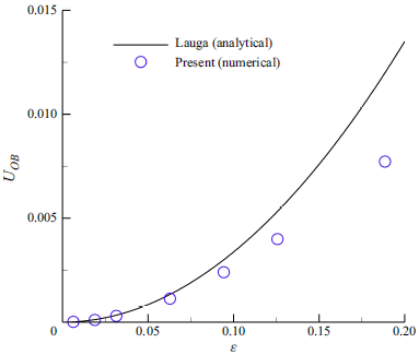
Free swimming speed
 $U_{\textit{OB}}$
for undulatory swimming motion in an OB fluid at small Reynolds number. These parameters are fixed:
 ${\textit{Re}}=0.0015$
,
 $\mu _r=2/3$
,
 ${\textit{Wi}}=6$
,
 $k_b = 80$
,
 $k_s = 1000k_b$
,
 $h=1/256$
,
 $\Delta t = 4 \times 10^{-7}$
,
 $\Delta s=4h$
.

In the end, the motion of Taylor’s swimming sheet is solved by
 \begin{align} {\frac {\partial \boldsymbol{X}}{\partial t}}=\boldsymbol{U}(s,t)=\int _{\varOmega _{\!f}}\boldsymbol{u}(\boldsymbol{x},t)\,\delta (\boldsymbol{X}(s,t)-\boldsymbol{x})\,\textrm{d}\boldsymbol{x}. \end{align}
To verify our numerical algorithm, we perform a benchmark case for the undulatory swimming motions in the OB fluids. As shown in figure 7, we measured the free swimming speed
 $U_{\textit{OB}}$
of an infinite swimmer at low Reynolds numbers, and compared the speed with the asymptotic results for Taylor’s swimming sheet of Lauga (Reference Lauga2007). We find that our results agree well with the analytical results at small amplitudes
 $\varepsilon \sim O(10^{-2})$
.
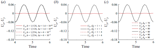
Next, we validate our numerical results by performing convergence tests for a swimmer free swimming in OB fluids, as demonstrated in figure 8. To model an infinite-length sheet in our simulations, it is placed within a square box with periodic boundary conditions. These tests investigate the time-dependent velocity components by varying the grid width, time step, domain size and bending stiffness. Our results demonstrate good agreement, confirming the reliability of the numerical approach.
Convergence studies of an infinite-length sheet free swimming in OB fluids with the time-dependent velocity
 $\boldsymbol{U}(U_x, U_y)$
by varying: (a) Eulerian grid width, (b) domain size, (c) the bending stiffness. These parameters are fixed:
 ${\textit{Re}}=0.0015$
,
 $\mu _r=0.3$
,
 ${\textit{Wi}}=3$
,
 $\varepsilon = 0.06$
,
 $k_s = 1000k_b$
.