1 Introduction
The flow over a wall-mounted finite circular cylinder is of considerable fundamental interest in fluid mechanics and widely encountered in numerous practical applications, such as cooler towers, chimneys and simplified buildings. Though the finite cylinder has a simple geometry, the flow over it is highly unsteady three-dimensionally. The complex vortex system around the finite cylinder consists of the horseshoe vortex at the wall junction, the tip vortex pair from the free end, the shedding vortex from the sidewalls, the mean arch vortex behind the cylinder, the trailing vortex around the reattachment zone, etc. Some sketches for these structures have been drawn in previous investigations (Kawamura et al. Reference Kawamura, Hiwada, Hibino, Mabuchi and Kumada1984; Pattenden, Turnock & Zhang Reference Pattenden, Turnock and Zhang2005; Frederich et al. Reference Frederich, Wassen, Thiele, Jensch, Brede, Hüttmann, Leder, Tropea, Jakirlic, Heinemann, Henke and Hönlinger2008; Porteous, Moreau & Doolan Reference Porteous, Moreau and Doolan2014), which provide a useful analysis framework for this type of flow. These three-dimensional flow structures were plausibly inferred from the previous flow visualizations and two-dimensional measurements, and a brief literature review is as follows:
(1) Tip vortex: in the literature, there were some differences in the origin of the streamwise tip vortex for the finite circular cylinder. For example, in the investigations of Etzold & Fiedler (Reference Etzold and Fiedler1976) and Kawamura et al. (Reference Kawamura, Hiwada, Hibino, Mabuchi and Kumada1984), it was indicated that the tip vortex originated from the leading edge of the free end. Roh & Park (Reference Roh and Park2003) showed that this vortex pair emanated from the focal points on the free-end surface. However, recent investigations (Pattenden et al. Reference Pattenden, Turnock and Zhang2005; Frederich et al. Reference Frederich, Wassen, Thiele, Jensch, Brede, Hüttmann, Leder, Tropea, Jakirlic, Heinemann, Henke and Hönlinger2008; Hain, Kähler & Michaelis Reference Hain, Kähler and Michaelis2008; Palau-Salvador et al. Reference Palau-Salvador, Stoesser, Fröhlich, Kappler and Rodi2010; Krajnović Reference Krajnović2011) by means of experiments and numerical simulations suggested that for the cases of the circular cylinder, this streamwise vortex pair originated from the trailing edge of the free end. The upwash flow from the sidewalls to the top area separates at the trailing edge of the free end, which triggers the formation of this tip vortex pair, as demonstrated by Palau-Salvador et al. (Reference Palau-Salvador, Stoesser, Fröhlich, Kappler and Rodi2010). In the results of large-eddy simulations (LES) by Krajnović (Reference Krajnović2011), an instantaneous tip vortex pair was observed slightly towards the wall due to the induced downwash. However, this vortex pair was not found in the instantaneous fields from the previous experimental measurements (Pattenden et al. Reference Pattenden, Turnock and Zhang2005; Hain et al. Reference Hain, Kähler and Michaelis2008) since the flow fields near the free end are highly unsteady three-dimensionally.
(2) Trailing vortex: the previous work revealed that the tip vortex pair only persisted downstream for a relatively short distance. For example, the tip vortex became hardly discernable at approximately
 $x/d=1.5$
(
 $x$
is streamwise location and
 $d$
is cylinder diameter) in the 2D-PIV results of Pattenden et al. (Reference Pattenden, Turnock and Zhang2005). Nevertheless, it is reported in the numerical simulation by Fröhlich & Rodi (Reference Fröhlich and Rodi2004) that a streamwise vortex pair existed at
 $x/d=3.5$
in the mean flow field. It is found that this streamwise structure, called the trailing vortex far from the free end, was not the continuation of the tip vortex, which has already disappeared. The trailing vortex results from the strong downwash effect and the associated upward motion away from the wake centreline triggered by the finite width of the cylinder (Frederich et al.
Reference Frederich, Wassen, Thiele, Jensch, Brede, Hüttmann, Leder, Tropea, Jakirlic, Heinemann, Henke and Hönlinger2008; Palau-Salvador et al.
Reference Palau-Salvador, Stoesser, Fröhlich, Kappler and Rodi2010). Practically, in the previous investigations, the trailing vortex was only shown in the mean flow field. Moreover, when extending downstream with a downward motion, the tip vortex may be connected to the trailing vortex, which needs a three-dimensional observation.
(3) Mean streamwise vorticity distribution: the base vortex generated behind the cylinder had the opposite sign to the tip vortex and induced an upwash flow away from the wall (Etzold & Fiedler Reference Etzold and Fiedler1976). The base vortex pair was weaker and dissipated more quickly than the tip vortex pair (Sumner, Heseltine & Dansereau Reference Sumner, Heseltine and Dansereau2004; Wang et al.
Reference Wang, Zhou, Chan and Lam2006). In the research of Sumner et al. (Reference Sumner, Heseltine and Dansereau2004) and Adaramola et al. (Reference Adaramola, Akinlade, Sumner, Bergstrom and Schenstead2006), the base vortex pair at the lee wall junction only occurred for
 $AR>3$
. Based on the previous investigations, Bourgeois, Sattari & Martinuzzi (Reference Bourgeois, Sattari and Martinuzzi2011) proposed two types of the mean streamwise vorticity distribution: the quadrupole type (two pairs of streamwise structures distributing in the upper and lower part of the wake, i.e. the tip and base vortex pairs) above a critical aspect ratio and the dipole type (one pair of the streamwise vortices located in the upper part) below the critical aspect ratio. In addition, Wang et al. (Reference Wang, Zhou, Chan and Lam2006) concluded that the appearance of the base vortex depended on the boundary-layer conditions, and the base vortex could be enhanced with increasing boundary-layer thickness, which was confirmed by later investigations (Wang & Zhou Reference Wang and Zhou2009; Hosseini, Bourgeois & Martinuzzi Reference Hosseini, Bourgeois and Martinuzzi2013). As observed by Hosseini et al. (Reference Hosseini, Bourgeois and Martinuzzi2013), the wake showed a quadrupole type for a thick boundary layer, and a dipole type for a thin boundary layer, although the aspect ratio (
 $AR=8$
) was higher than 3. Later, an experimental investigation was conducted by Hassan, Bourgeois & Martinuzzi (Reference Hassan, Bourgeois and Martinuzzi2015) on the interaction between the horseshoe vortex system (HVS) and the wake field behind a square cylinder (
 $AR=4$
) for two cases of the turbulent boundary layer (
 $\unicode[STIX]{x1D6FF}/h=0.18$
and 0.64,
 $\unicode[STIX]{x1D6FF}$
is boundary layer thickness and
 $h$
is cylinder height). It was found that for the thick boundary layer, the whole wake appeared to be affected by the HVS dynamics. Based on the existing studies for
 $AR>3$
, they concluded that a dipole-type mean wake was observed to occur when
 $\unicode[STIX]{x1D6FF}/d<1$
and a quadrupole type for
 $\unicode[STIX]{x1D6FF}/d>1.3$
. It remains unclear which type would be observed for
 $AR<3$
in the case of the thick boundary layer. Specifically, we need to address the following question: for the short cylinder, does the aspect ratio or the thickness of the boundary layer dominate the wake behaviour?
(4) Spanwise vortex shedding: the vortex shedding on the sidewalls of the finite cylinder was significantly influenced by the aspect ratio due to the effects of the free end and the base wall (Lee Reference Lee1997; Fröhlich & Rodi Reference Fröhlich and Rodi2004; Pattenden et al.
Reference Pattenden, Turnock and Zhang2005; Palau-Salvador et al.
Reference Palau-Salvador, Stoesser, Fröhlich, Kappler and Rodi2010; Tsutsui Reference Tsutsui2012). In addition, with PIV measurements on a square cylinder, Wang et al. (Reference Wang, Zhou, Chan and Lam2006) suggested that the boundary-layer conditions also had a great influence upon the occurrence of antisymmetrically and symmetrically arranged vortices. It is reported that increasing
 $\unicode[STIX]{x1D6FF}/h$
could enhance the base vortex and induced upwash flow, and the shedding type was closely related to the downwash and upwash effect. This relation was confirmed by Wang & Zhou (Reference Wang and Zhou2009), and it was concluded that the downwash/upwash flow promoted the symmetric vortex shedding. Thus, there exist both types of vortex shedding along the cylinder span in the meantime, which was supported by the proper orthogonal decomposition (POD) analysis for the flow field behind a square cylinder of
 $AR=7$
by Wang, Cao & Zhou (Reference Wang, Cao and Zhou2014a
). In their investigation, it was indicated that the flow at
 $x/d=6$
(near the top) was dominated by symmetric vortex shedding, while at
 $x/d=3.5$
and 1 (i.e. the centre and lower part, respectively), the wake was dominated by the alternating spanwise vortex shedding.
(5) Arch vortex: as sketched by Lee (Reference Lee1997), the arch vortex occurred for the cases of
 $AR<3$
. Practically, in the previous investigations (Fröhlich & Rodi Reference Fröhlich and Rodi2004; Frederich et al.
Reference Frederich, Wassen, Thiele, Jensch, Brede, Hüttmann, Leder, Tropea, Jakirlic, Heinemann, Henke and Hönlinger2008; Krajnović Reference Krajnović2011), the arch vortex was only observed in the mean wake field. With LES for
 $AR=2.5$
, Fröhlich & Rodi (Reference Fröhlich and Rodi2004) conjectured that an arch vortex, with the shape of a reversed
 $U$
located behind the cylinder, was a feature of the time-averaged but not the instantaneous flow. Later, the simulations by Krajnović (Reference Krajnović2011) showed that the legs of the mean arch vortex were inclined to the cylinder axis in the streamwise direction for
 $AR=6$
and the angle of inclination was approximately
 $31^{\circ }$
. It is not clear for the cases of the short cylinder. The downwash effect dominates the whole wake for the lower aspect ratio (
 $AR<3$
), which means a greater possibility of symmetric vortex shedding (Wang et al.
Reference Wang, Cao and Zhou2014a
). The formation of the arch vortex is closely related to the shedding modes. One could conjecture reasonably that symmetric vortex shedding might induce the occurrence of the instantaneous arch vortex for the short cylinder. In addition, the shape of the mean arch vortex remains unclear if considering the tip vortex and associated downwash effect.
(6) Flow structure model: the relations among the typical structures mentioned above have also been discussed in the literature. From the isolated 2D-PIV measurements, Wang & Zhou (Reference Wang and Zhou2009) proposed a physical model for the flow structures behind a finite-square cylinder (
 $AR=3{-}7$
). This topological model showed that a single arch-type coherent structure occurred in the near wake, which was the combination of the tip, base and spanwise vortex. The model has not been confirmed by later studies. Developing a new phase-averaged technique for the reconstruction of 3D velocity fields from the 2D-PIV data, Bourgeois et al. (Reference Bourgeois, Sattari and Martinuzzi2011) proposed a novel topological pattern in which an alternating shedding half-loop structure was observed for a square cylinder of
 $AR=4$
. This half-loop structure was characterized by a vertical principal core and a streamwise connector strand. The originally vertical vortex (i.e. the principal core) from the sidewalls deformed to create the streamwise structures. This streamwise connector strand connected upstream to the opposite sidewall structures, which induced the formation of the half-loop structures. Since then, many numerical simulations (Moazamigoodarzi et al.
Reference Moazamigoodarzi, Bergstrom, Einian and Sumner2014; Saeedi, Lepoudre & Wang Reference Saeedi, Lepoudre and Wang2014; Wang, Jackson & Sui Reference Wang, Jackson and Sui2014b
; Saeedi & Wang Reference Saeedi and Wang2016) have supported the existence of the half-loop structure for the same cylinder configuration.
(7) Obstacle shape effect: moreover, it is worth pointing out that there exist some differences between circular- and square-cylinder wakes. For example, an evident shedding signal was observed near the free end for the square cylinders (Wang & Zhou Reference Wang and Zhou2009; Bourgeois et al. Reference Bourgeois, Sattari and Martinuzzi2011; Hosseini et al. Reference Hosseini, Bourgeois and Martinuzzi2013), while the shedding signal was difficult to identify for the circular cylinders (Park & Lee Reference Park and Lee2002; Sumner et al. Reference Sumner, Heseltine and Dansereau2004; Adaramola et al. Reference Adaramola, Akinlade, Sumner, Bergstrom and Schenstead2006; Hain et al. Reference Hain, Kähler and Michaelis2008; Krajnović Reference Krajnović2011). Furthermore, the explanation of the tip vortex appears to be different for the two cylinder configurations. For the square cylinder, the streamwise vorticity near the free end came from reorientation of the initially vertical vorticity in the sidewall shear layers due to lateral vorticity of the free-end shear layer, i.e. the tip vortex is the deformation of the Karman vortex. However, for the circular cylinder, the tip vortex originates from the trailing edge of the free end, as mentioned above, and is not a representation of the Karman vortex. Practically, the separation location is fixed at the sharp edge for the square obstacle, while it is not the case for the circular obstacle. Naturally, the obstacle wake behaviour is different between the two cylinder cases.
Although a number of investigations have been conducted for this type of flow, there still exist some questions that need to be clarified, especially for the short cylinder. Particularly, the spatial locations of the typical vortex structures and their interactions are yet to be clarified. So far, few studies have been focused on experimentally obtaining the instantaneous volumetric vortex structures. It may be the reason that the measurement volume for the wake field is relatively large, and thus an enormous storage memory in the data acquisition devices will be required for the 3D velocity field calculations. Indeed, the wake structures show strong three-dimensional characteristics, so that with the planar measurement techniques, some important information concerning the flow field might be missed. The 3D finite-square-cylinder wake field which was deduced from the planar measurements has been elaborated by Wang & Zhou (Reference Wang and Zhou2009) and Bourgeois et al. (Reference Bourgeois, Sattari and Martinuzzi2011), while the understanding of the 3D wake for circular cylinders is still quite limited, except for the simulation work by Krajnović (Reference Krajnović2011). In particular, there are some questions concerning the flow over circular cylinders compared with the results for square cylinders. For example, considering the differences in the wake behaviour behind circular and square cylinders, does the half-loop structure also occur for the circular cylinder cases? The main intention here is to investigate the volumetric vortex structures, especially the instantaneous ones, in the short-cylinder wake. In addition, the present work attempts to improve the current conceptual model, in which the vortex structures and their relations will be described in more detail. For this object, tomographic PIV (Elsinga et al. Reference Elsinga, Scarano, Wieneke and van Oudheusden2006) is employed to measure the instantaneous flow field. Furthermore, the developments and dynamic characteristics of these volumetric wake vortices could be explored. Accordingly, in the present paper, POD and other statistical analysis methodologies will be used in the whole three-dimensional wake field.
This paper is constructed as follows. In § 2, detailed information of the experimental set-up and the measurement parameters for the TPIV system will be described. Section 3 presents the basic mean flow field. In § 4, the averaged and instantaneous typical flow structures in the wake field are presented with the aid of vortex identification methods, and some novel experimental results are displayed. Moreover, a new sketch of the mean flow field is obtained in § 4.2. A POD analysis for the whole wake field is performed in § 5. The emphasis is laid on the periodicity of the primary structures and the statistics of the antisymmetric and symmetric wake behaviours. We will end this paper with conclusions in § 6.
2 Experimental set-up and measurement technique
The experiment was conducted in a circular open water tunnel in Beijing University of Aeronautics and Astronautics, China. In order to enable experiments with the optical measurements, the bottom and two sidewalls of the test section are made of Plexiglass. Before entering the contraction section, the flow passes through a set of two honeycombs with a slenderness ratio of 7.5 and two screens with 60 mesh stainless steel grids. The width of the contraction section inlet is 2000 mm and the contraction ratio in width is 3.3:1. The size of the test section is 3000 mm (length)
 $\times$
600 mm (width)
 $\times$
700 m (height). The working section is followed by a diffuser with a diffusion half-angle of
 $4^{\circ }$
and a power unit. The free-stream velocity
 $U_{\infty }$
can be adjusted up to
 $500~\text{mm}~\text{s}^{-1}$
with a motor controller.
2.1 Experimental set-up
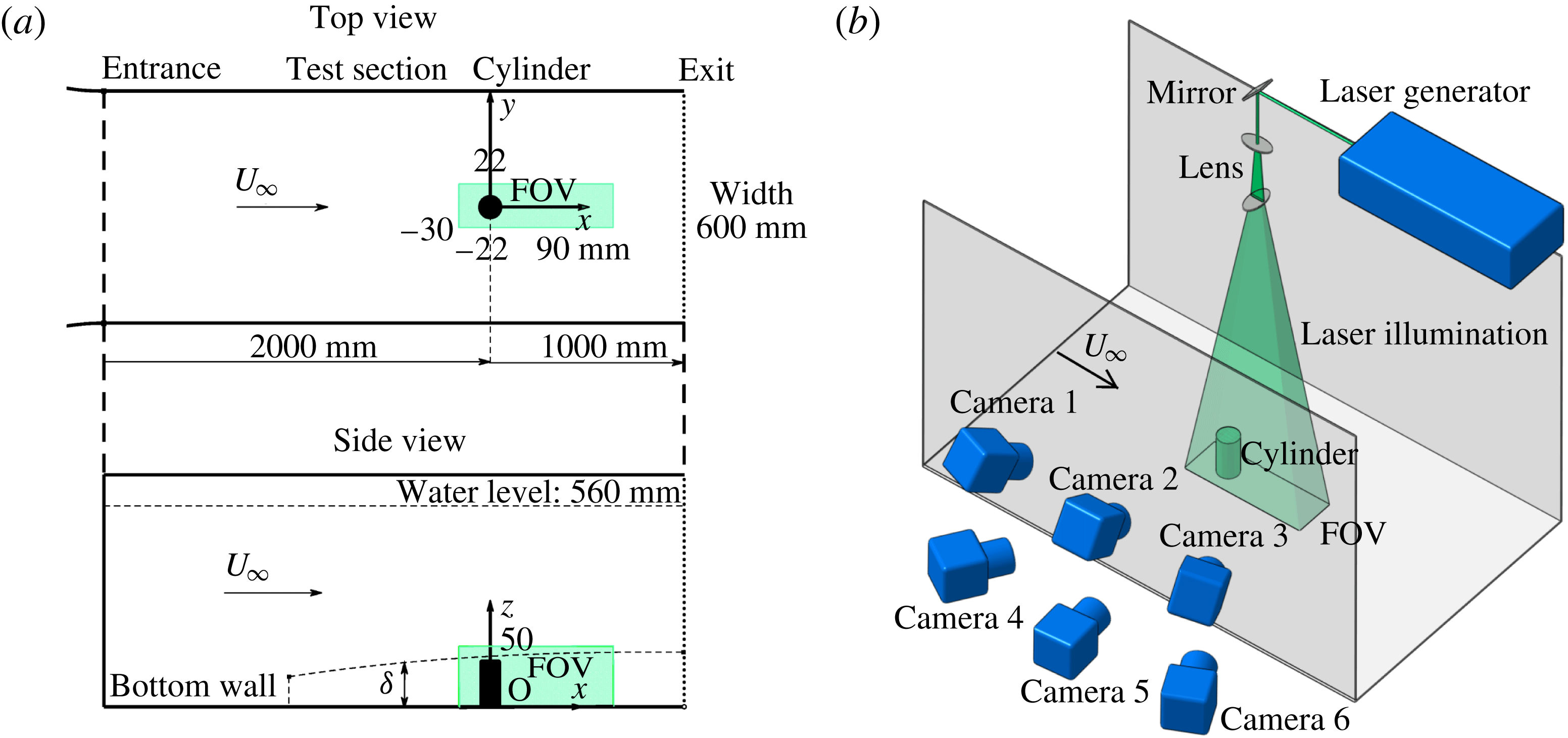
(a) Experimental arrangement in the water tunnel with the definition of the coordinate system, field of view (FOV) and corresponding essential parameters; (b) sketch of the experimental set-up for tomographic PIV measurements with the camera and illumination arrangements.

The sketch of the experimental set-up is given in figure 1. The circular cylinder model was mounted on the central axis of the bottom wall 2000 mm downstream of the test section entrance. The model has an aspect ratio of
 $AR=h/d=2$
with diameter
 $d=20~\text{mm}$
. To reduce reflections and interference from background light in the camera images, this steel cylinder was painted black. The experiment was conducted at a free-stream velocity of
 $U_{\infty }=160~\text{mm}~\text{s}^{-1}$
, giving a Reynolds number (based on the cylinder diameter) of
 $Re_{d}=U_{\infty }d/\unicode[STIX]{x1D708}=3,830$
, where
 $\unicode[STIX]{x1D708}$
is the kinematic viscosity of the fluid. Equipped with a tripwire at the test section entrance, a turbulent boundary layer was produced. The velocity profile was measured at the location of the finite cylinder using two-dimensional time-resolved particle image velocimetry (2DTRPIV). At the location of the cylinder, the undisturbed boundary-layer thickness
 $\unicode[STIX]{x1D6FF}$
was 41.0 mm (
 $\unicode[STIX]{x1D6FF}/h=1.025$
), resulting in the cylinder being fully immersed in the turbulent boundary layer. The measured shape factor (
 $H$
) was 1.38, which indicated the turbulent flow regime in the boundary layer. Relevant properties of the boundary layer are summarized in table 1. As shown in figure 1(a), along with the coordinate system, the origin of the coordinate system was set at the centre of the cylinder bottom surface. The three axes (
 $x$
,
 $y$
,
 $z$
) were along the streamwise, spanwise and wall-normal directions, respectively. Hollow glass beads with diameters in the range
 $15{-}20~\unicode[STIX]{x03BC}\text{m}$
and a density of
 $1.05\times 10^{3}~\text{kg}~\text{m}^{-3}$
were seeded as tracers in the present experiment. The response time of the seeding particles based on the free-stream velocity was
 $1.6{-}2.8\times 10^{-5}~\text{s}$
, which indicated good following performance of the particle tracers. The experimental apparatus for the tomographic PIV measurements is shown in figure 1(b). Illumination was provided by a dual-head Nd : YAG laser (
 $500~\text{mJ}~\text{pulse}^{-1}$
, 532 nm wavelength) with a pulse separation time of 3 ms, which yields average displacements of approximately 0.48 mm (8 pixels) in the free-stream region. The optical lenses and the mirror were designed to generate a 45 mm thick light sheet illuminating the tracer particles around the finite cylinder. The light sheet was perpendicular to the test section bottom. To improve the accuracy of the measurement, six high-resolution (
 $2058\times 2456~\text{pixels}^{2}$
, 12bit) double-exposure CCD cameras (IM-PERX B2520) were applied to record the measurement domain simultaneously. The sensor was cropped in the wall-normal direction, resulting in an active sensor region of
 $1100\times 2456~\text{pixels}^{2}$
. In figure 1(b), the viewing angles were approximately
 $60^{\circ }$
between Camera 1 and 3, and
 $30^{\circ }$
between Camera 2 and 5, which led to a high reconstruction quality (Scarano Reference Scarano2013). 50 mm Nikon lenses with an aperture of f/8.0 was positioned approximately 810 mm distant from the measurement domain to shoot images. Therefore, the DOF (depth of focus) of the lens was approximately 108 mm, 2.5 times the thickness of the measurement volume (44 mm). On account of the above conditions, all particles in the measurement area were recorded in focus, with no need for lens-tilt adapters mentioned in the Scheimpflug condition (Prasad & Jensen Reference Prasad and Jensen1995). The timing of the laser, cameras and frame grabber was controlled by a synchronizer. The sampling frequency for this measurement was 5 Hz, which indicated five pairs of images recorded per second for every camera. The frequency of vortex shedding was estimated to be approximately 1.6 Hz based on the dimensionless frequency (
 $St=0.21$
) for the infinite cylinder at the subcritical Reynolds number, so that the frequency of 5 Hz can resolve the periodic features present. Five data sets, in which the number of image pairs in every set was 200, were acquired and the results from these five datasets were in good agreement. The results shown in the present paper come from these 1000 three-dimensional, three-component (3D3C) independent instantaneous vector fields.
Details of the boundary layer at the position of the cylinder model.

2.2 Calculation for tomographic PIV
Tomographic particle image velocimetry (TPIV) was applied in the present investigation for its ability to display the average and instantaneous three-dimensional distribution of velocity and vorticity.
Generally, two main steps are necessary in a traditional TPIV process. First, the reconstruction of the particle intensity distribution is performed based on a mapping function between the image and the object space. Second, the calculation of the 3D3C vector fields is conducted through the three-dimensional cross-correlation. Before the volume reconstruction, constant background needs to be removed from the raw particle images. The TPIV process is implemented by an in-house MATLAB code, which is based on the algorithms and principles of the methodology described by Elsinga et al. (Reference Elsinga, Scarano, Wieneke and van Oudheusden2006). The MART algorithm with four iterations and a voxel-to-pixel rate of 1 was applied to reconstruct the three-dimensional particle intensity field. The measurement volume shown in figure 1(a) was in the coordinate range [
 $-30,90$
]
 $\times$
[
 $-22,22$
]
 $\times$
[0, 50] (mm), so that its corresponding physical domain had a size of
 $120\times 44\times 50~\text{mm}^{3}$
(
 $6d\times 2.2d\times 2.5d$
) that contained the whole finite cylinder. Resulting from the reconstruction process, the volume size was
 $2000\times 733\times 883~\text{voxel}^{3}$
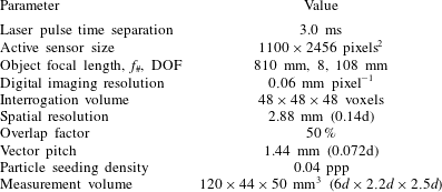
in the image domain, with a digital imaging resolution of 0.06 mm per pixel. The 3D vector calculation was done through multi-pass correlation analysis (Scarano Reference Scarano2002) with a deforming interrogation window. In the final pass, the interrogation volume was
 $48\times 48\times 48$
voxel with 50 % overlap, leading to a spatial resolution of 2.88 mm (0.14
 $d$
) and a vector pitch of 1.44 mm (0.072
 $d$
). The resulting spatial resolution enabled the detection of the large-scale vortex structures as their scales were on the order of
 $2d$
in the present work. Post-processing of the 3D vector field was performed by a divergence-free smoothing algorithm (Wang et al.
Reference Wang, Gao, Wang, Wei, Li and Wang2016a
). The six-camera system reconstructed the images with a seeding density of 0.04 ppp (particles per pixel) that was calculated by counting the intensity peaks in the images. Approximately six particles were found within an interrogation box, which was feasible for a robust cross-correlation analysis (Scarano Reference Scarano2013). The measurement and calculation parameters for TPIV are summarized in table 2.
Measurement and calculation parameters for TPIV.
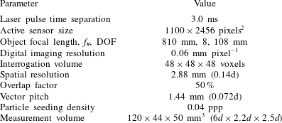
The experimental uncertainty arising from the measurement error is connected to the tomographic PIV measurement. The uncertainty in the mean flow fields depends on the number of uncorrelated samples
 $N_{s}$
and the fractional fluctuation
 $\unicode[STIX]{x1D70E}_{u}=u^{\prime }/U_{\infty }$
, which is the normalized standard deviation. In the present study, the dataset consisted of 1000 independent instantaneous flow fields and the typical level of normalized streamwise velocity fluctuations
 $\unicode[STIX]{x1D70E}_{u}$
in the turbulent boundary layer is approximately 0.1. The uncertainty in the mean field could be estimated by
 $\unicode[STIX]{x1D700}_{u}=\unicode[STIX]{x1D70E}_{u}/\sqrt{N_{s}}$
. Thus, for the present experiment,
 $\unicode[STIX]{x1D700}_{u}\approx 0.003$
. Accordingly, the uncertainty in the root mean square of the velocity fluctuation is
 $\unicode[STIX]{x1D700}_{u^{\prime }}\approx 0.002$
, which is estimated by
 $\unicode[STIX]{x1D700}_{u^{\prime }}=\unicode[STIX]{x1D70E}_{u}/\sqrt{2(N_{s}-1)}$
. The uncertainty due to the data processing algorithm (e.g. the reconstruction and the cross-correlation algorithm) is another source and controlled by the efforts from previous studies (see Elsinga et al. (Reference Elsinga, Scarano, Wieneke and van Oudheusden2006), Wieneke (Reference Wieneke2008) and Scarano (Reference Scarano2013), for a few examples). Additional sources of unquantified experimental random error include background illumination, camera background noise and the refractive index mismatch. Volume self-calibration was applied to improve the accuracy of the mapping function (Wieneke Reference Wieneke2008), reducing the regular disparity error of the original mapping function to less than 0.1 pixel. Following Elsinga et al. (Reference Elsinga, Scarano, Wieneke and van Oudheusden2006), the uncertainty for the vector was estimated as less than 0.2 pixel, corresponding to 2.5 % of the free-stream velocity (
 $U_{\infty }$
). In addition, the six-camera configuration in the present experiment attained a higher accuracy than the four-camera system. Overall, the accuracy of the experimental procedure was adequate for the present investigation.
In this paper, the velocity and vorticity were normalized by the free-stream velocity
 $U_{\infty }$
and
 $U_{\infty }/d$
, respectively. In order to observe the target structures much more clearly in the present investigation, a Gaussian smoothing with a
 $3\times 3\times 3$
spatial kernel and a coefficient of
 $\unicode[STIX]{x1D70E}=0.75$
was performed to remove residual noise and small structures in the instantaneous non-dimensional vorticity and other volumetric data fields.
3 Basic mean flow field
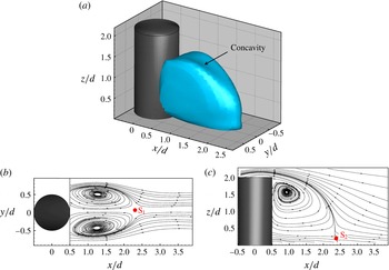
The wake behind the finite cylinder shows an apparent characteristic of the complex three-dimensional separation flow. The isosurface of
 $\bar{u}/U_{\infty }=0$
is displayed in figure 2(a), which represents the 3D-contour recirculation zone in the time-averaged flow field (average over
 $N=1000$
snapshots). Along the plane of symmetry,
 $y/d=0$
, a small concavity (i.e. the lower area on the surface) is observed in this isosurface, which is induced by the strong downwash flow from the free end. A similar phenomenon was displayed by Leder (Reference Leder2003) with a three-component laser Doppler anemometer (LDV). Moreover, due to the free-end effect, the extension of the recirculation zone shrinks in the
 $z$
direction and the recirculation disappears at elevations larger than
 $z/d=1.6$
. It means that the downwash flow impinges on the shedding process near the free end from the sidewalls of the cylinder. In figure 2(b,c), two cross sections at
 $z/d=0.6$
and
 $y/d=0$
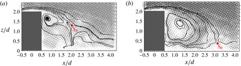
are displayed with mean streamlines to show the details of the mean wake field. The two figures show clearly the separation flow from the sidewalls and the free end, which resemble the flow around a 2D bluff body and over the backward-facing step, respectively. It is noteworthy to point out that the flow studied here is not simply the combination of these two planar flows but has a highly three-dimensional feature, as shown in the instantaneous flow fields discussed later. Two saddle points,
 $\text{S}_{1}$
in figure 2(b) and
 $\text{S}_{2}$
in figure 2(c), are apparent in the mean streamline pattern. Both of them indicate closure of the separation region in the near wake. As evident in figure 2(b), two large counter-rotating vortices in the rear region of the obstacle are observed. The recirculation from the free end in figure 2(c) is spread over most of the height of the finite cylinder. The downwash flow from the free end approaches the wall and ceases at the saddle point
 $\text{S}_{2}$
. This result is consistent with previous knowledge where the downwash effect dominates the wake for
 $AR<3$
. The location of
 $\text{S}_{2}$
is at
 $x/d=2.38$
and
 $z/d=0.2$
, which is influenced by the boundary-layer conditions and the aspect ratio.
Mean recirculation zone in the near wake. (a) Isosurface of
 $\bar{u}/U_{\infty }=0$
. The
 $x$
–
 $y$
slice (b) at
 $z/d=0.6$
and the
 $x$
–
 $z$
slice (c) at
 $y/d=0$
are displayed with mean streamlines. The two saddle points are marked with the red dots.

4 Typical wake structures
The effects of the free end and the cylinder-wall junction trigger the three-dimensional dynamic characteristics of the finite-cylinder wake. Various vortex patterns occur in the wake, and these typical flow structures include the horseshoe vortex wrapping around the front junction (not shown in this paper), the separation vortex from the sidewalls of the cylinder, the tip vortex originating from the free end and the mean arch vortex in the near-wake region. These three-dimensional structures, which were conjectured from the flow visualizations and planar measurements in the reported experimental studies, are first experimentally confirmed in the present investigation. Moreover, new structures and phenomena were observed in both the time-averaged and instantaneous flow fields, which will be shown in the following details.
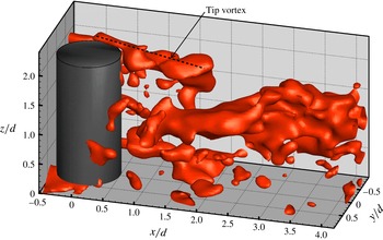
Instantaneous streamwise vorticity field at
 $t=1.0~\text{s}$
(isosurface of
 $\unicode[STIX]{x1D714}_{x}d/U_{\infty }=1$
). The positive tip vortex in the region of
 $y/d<0$
is marked by the black dotted line.

4.1 Tip vortex originating from the free end
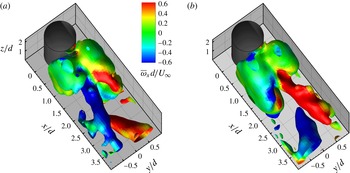
The tip vortex was clearly observed in the instantaneous flow field. In figure 3, the instantaneous dimensionless streamwise vorticity isosurface of
 $\unicode[STIX]{x1D714}_{x}d/U_{\infty }=1$
is presented, where
 $\unicode[STIX]{x1D714}_{x}$
is the streamwise vorticity. The black dotted line labels a positive tip vortex located in the region
 $y/d<0$
. The negative tip vortex is omitted to allow a clearer observation. As shown in the figure, the tip vortex pair, originating from the trailing edge of the free end, was relatively weak in strength and did not persist downstream for a long distance (
 $x/d<2$
). When developing downstream, this vortex pair inclines towards the ground plane due to the downwash effect, and then disappears. In addition, it is found that when being observed frame by frame, this instantaneous tip vortex pair evidently shows unsteadiness and irregularity in terms of its symmetry and strength, similar to observations of the flow on the free-end surface using tomographic and time-resolved PIV by (Hain et al.
Reference Hain, Kähler and Michaelis2008).
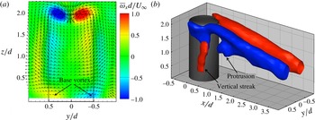
Figure 4(a) shows the time-averaged wake field in the
 $y$
–
 $z$
section for
 $x/d=0.85$
with the streamwise vorticity contour and the overlapped velocity vectors, in which the tip vortex is clearly observed. The velocity field shows a strong downwash effect along the wake centreline near the free end. Recirculation occurs with the upward-directed flow in the middle height of cylinder. At the sides of the cylinder on this slice, weak vorticity is observed due to the flow spreading outside the wake. In addition to the tip vortex pair in this figure, a base vortex pair is observed near the wall behind the cylinder, which is triggered by the present thick boundary layer (Wang et al.
Reference Wang, Zhou, Chan and Lam2006). It is noted that this vortex pair is much weaker and more short-lived (extending downstream only for half-diameter) than the tip vortex pair (see the colour depth). It should be mentioned that this base vortex pair should not be confused with the horseshoe vortex, since the horseshoe vortex does not extend into the wake and has the opposite sign to the base vortex.
Figure 4(b) shows the 3D mean streamwise vorticity isosurface of
 $\bar{\unicode[STIX]{x1D714}}_{x}d/U_{\infty }=\pm 0.5$
, coloured with blue and red representing the negative and positive vortex, respectively. A pair of evident streamwise vortices originate from the trailing edge of the free end. Ostensibly, this streamwise vortex distribution shows a dipole type. Previous knowledge (Sumner et al.
Reference Sumner, Heseltine and Dansereau2004; Adaramola et al.
Reference Adaramola, Akinlade, Sumner, Bergstrom and Schenstead2006; Sumner & Heseltine Reference Sumner and Heseltine2008) suggested that the streamwise vorticity was distributed in a quadrupole type above a critical aspect ratio and a dipole type below the critical aspect ratio for finite circular cylinders. Hassan et al. (Reference Hassan, Bourgeois and Martinuzzi2015) found that
 $\unicode[STIX]{x1D6FF}/d$
is a significant parameter determining the observed wake topology due to the interaction between the HSV and shed vortices, and concluded that the thicker boundary layer gave rise to a greater probability of the quadrupole type. Though the boundary layer is thick in the present experiment, the wake shows a dipole type because the base vortex pair is relatively weak. The observation of the dipole topology for the present condition (
 $AR=2$
,
 $\unicode[STIX]{x1D6FF}/d=2.05$
) appears to suggest that for
 $AR<3$
, the effect of the aspect ratio is more dominant than the effect of the thick boundary layer. It should be mentioned that the red vertical streak in figure 4(b) corresponds to positive streamwise vorticity due to the reversed flow in the mid-height of the cylinder sidewalls in figure 4(a). Based on observations of figures 3 and 4(b), the formation of the tip vortex can be determined as follows. Near the free end, the flow from the sidewalls of the cylinder has an upward motion, which is clearly observed in the hydrogen bubble flow visualization (not shown in the present paper). When this flow passes over the trailing edge of the free end, separation occurs and triggers the formation of the tip vortex pair.
Average streamwise vorticity field. (a)
 $y$
–
 $z$
slice at
 $x/d=0.85$
coloured by the streamwise vorticity with in-plane velocity vectors overlapped. The dashed line denotes the finite cylinder. (b) Streamwise vortex with the isosurface of
 $\bar{\unicode[STIX]{x1D714}}_{x}d/U_{\infty }=\pm 0.5$
(‘
 $-$
’ in blue and ‘
 $+$
’ in red).

As discussed above, the tip vortex is a short-lived structure (extension length
 $x/d<2$
). However, the streamwise vortex shown in figure 4(b) extends downstream to the end of the measurement domain. Similarly, Fröhlich & Rodi (Reference Fröhlich and Rodi2004) found that the streamwise vortex pair appeared at
 $x/d=3.5$
in the time-averaged flow of their LES results. They considered the tip vortex had already disappeared at this location and attributed this phenomenon to the formation of the trailing vortex. This trailing vortex pair was not the continuation of the tip vortex, though both of them had the same sign. The trailing vortex forms due to the strong velocity gradient between the strong downwash flow and the outside flow of the wake. From figure 4, it is concluded that connection (or mergence) between the tip vortex and trailing vortex occurs for an aspect ratio of 2 in the present experiment.
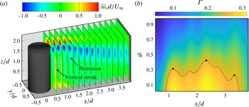
Strength variation of the mean streamwise vortex in the
 $x$
-direction: (a) 14 slices from
 $x/d=0.5$
to
 $x/d=3.9$
showing the variation of the
 $x$
-vorticity magnitude; (b) development of the in-plane circulation. The ordinate Percentage represents the percentage of the local maximum of
 $\unicode[STIX]{x1D706}_{ci}$
and indicates the boundary of the integral domain
 $A$
. It is indicated that the development of the circulation in the
 $x$
-direction is evident in the case of the most local circulation (i.e. percentage
 ${<}30\,\%$
) contained inside the boundary of
 $A$
. The black dashed line denotes
 $\unicode[STIX]{x1D6E4}=0.26$
. The three black dots correspond to the peaks at
 $x/d=1.2$
, 2.35 and 3.35, respectively.

To investigate this connection, the development of streamwise vorticity in the
 $x$
-direction was discussed. Fourteen
 $y$
–
 $z$
slices from
 $x/d=0.5$
to
 $x/d=3.9$
are displayed with the streamwise vorticity contour in figure 5(a). It is shown that this streamwise vortex structure becomes dispersed in area when extending downstream. The vortex strength shows evident alternating variation in the form of the colour intensity. In addition, the vertical streak and the protrusion are also shown in this figure, corresponding to figure 4(b). In order to confirm this variation of the vortex strength, tracking of the circulation referring to the vortex flux was performed. The circulation
 $\unicode[STIX]{x1D6E4}$
is calculated by
 $$\begin{eqnarray}\unicode[STIX]{x1D6E4}=\int _{A}\unicode[STIX]{x1D714}_{x}\,\text{d}A,\end{eqnarray}$$
where
 $A$
is the domain of integration. The boundary of the integral domain
 $A$
was defined as the percentage of the local maximum of
 $\unicode[STIX]{x1D706}_{ci}$
, which is the imaginary part of the complex conjugate eigenvalue of the velocity gradient tensor (VGT,
 $\unicode[STIX]{x2202}u_{i}/\unicode[STIX]{x2202}x_{j}$
) and represents the swirling strength (Zhou et al.
Reference Zhou, Adrian, Balachandar and Kendall1999). Considering the influence of the choice of the percentage, the circulation tracking results at different percentages have been drawn in figure 5(b). When most of the circulation is contained in the integral domain, the development can be clearly determined. Specifically in figure 5(b), a lower percentage corresponds to a larger integral domain
 $A$
and more local circulation contained inside the boundary. Therefore, at a certain low percentage (e.g. 10 %), we can observe development of the circulation in the streamwise direction. Due to a continuous feed of shear layers near the free end, the circulation increases and reaches its maximum at approximately
 $x/d=1.2$
, as shown by the first black dot in figure 5(b). In the following, the circulation experiences a decline in the streamwise direction. The reason for this decline is understandable, as the free-end shear layer become weak away from the free end. It is clearly indicated that there are three peaks at
 $x/d=1.2$
, 2.35 and 3.35, respectively. In addition, a small peak occurs at approximately
 $x/d=1.7$
, which is attributed to the appearance of the protrusion shown in figures 4(b) and 5(a). The peak at
 $x/d=2.35$
in the reattachment zone is attributed to the formation of the trailing vortex and its connection with the residual tip vortex, while it is not clear for the peak at
 $x/d=3.35$
. However, this peak may be ascribed to the deflection and uplift of the large-scale streamwise vortex shown in figure 3, which will be further discussed in § 4.3. It is noted that this variation in circulation shows good agreement with the maps of the vorticity contour in figure 5(a). Combined with the analysis on figures 4 and 5, the vortex evolution and connection can first be determined in the present experiment. The tip vortex is uplifted immediately, originating from the trailing edge with an increase in strength. Then, this vortex pair is directed to the ground wall due to the downwash effect with decreasing strength. The connection between the residual weak tip vortex pair and the trailing vortex occurs around the reattachment zone, which makes the vortex strength increase and reach a peak at
 $x/d=2.35$
. The connected structures become weak when continuously convecting downstream. The formation, development and connection of the mean tip and trailing vortex will be viewed in the sketch shown at the end of § 4.2.
4.2 Arch vortex near wake
The existence of the arch vortex in the finite-cylinder wake had not been experimentally confirmed in previous investigations due to limitations of the planar measurement. This arch vortex structure is observed in this experiment, and its main features are acquired and shown as follows.
In this investigation, the
 $Q$
criterion (Hunt, Wray & Moin Reference Hunt, Wray and Moin1988), in which
 $Q$
is calculated by
 $$\begin{eqnarray}Q=(\Vert \unicode[STIX]{x1D6FA}\Vert ^{2}-\Vert S\Vert ^{2})/2,\end{eqnarray}$$
was employed to identify the vortex structures.
 $\unicode[STIX]{x1D6FA}$
and
 $S$
here are the symmetric and antisymmetric components of the VGT, representing the angular velocity tensor and the rate of strain tensor, respectively.
 $\Vert \,\Vert$
represents the Euclidean norm. The
 $Q$
criterion identifies the vortices in the case of excess rotation relative to the strain rate (i.e. the positive second invariant
 $Q$
of VGT). Based on (4.2),
 $Q$
is normalized by the square of
 $U_{\infty }/d$
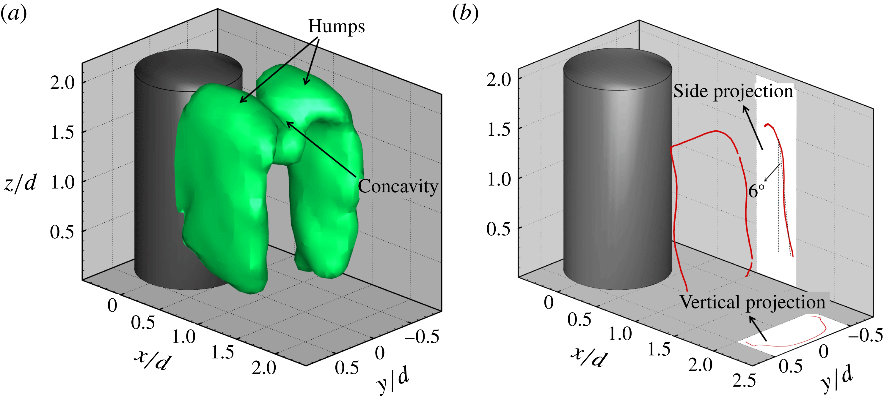
. Figure 6(a) presents the isosurface of
 $Q/(U_{\infty }/d)^{2}=0.40$
in the mean flow field. The arch structure is nicely observed and appears to be the shape of an M instead of a reversed U (Fröhlich & Rodi Reference Fröhlich and Rodi2004) located over the ground plane behind the finite cylinder. The legs of this M-shape structure are almost vertical to the ground plane. As evident in this figure, a concavity (or groove) in this M-shape structure is observed near the free end. There are two reasons behind this sunken phenomenon. First, the downwash flow coming from the free end pushes the vortex structures downward along the wake centreline. Second, two humps (naturally a concavity between them) of this M-shape structure result from the tip vortex being contained in this structure. Indeed, Fröhlich & Rodi (Reference Fröhlich and Rodi2004) mentioned that the arch vortex might exhibit a different shape in its upper part due to the existence of the tip vortex, which is corroborated by the present results. In addition, if the contour value of
 $Q$
is reduced in figure 6(a), there will exist two evident streamwise structures, the same as the observation in figure 4(b). Again, it is suggested that the long streamwise vortex pair is relatively weak. Moreover, the existence of a tip vortex is the reason why the shape of the vortex structure extracted by the
 $Q$
criterion is different from the one displayed by the vortex-core-extracting method discussed below.
Mean arch vortex structure with (a) the isosurface of
 $Q/(U_{\infty }/d)^{2}=0.40$
and (b) the vortex filaments constituted by the vortex cores attached by the vertical and side projections.

In order to have better knowledge of this arch structure, another way to present it was used by extracting vortex cores. The vortex filament was extracted based on the critical point theory (Sujudi & Haimes Reference Sujudi and Haimes1995). As evident in figure 6(b), the vortex filament constituted by vortex cores shows an arch shape. Vertical and side projections are provided to display more details of the arch vortex. Different from the M-shape structure displayed by the isosurface of dimensionless
 $Q$
, the vortex filament has a perfect arched shape, with its legs inclined slightly and its head (i.e. the horizontal part) stretched upstream. The head of the arch structure is pulled upstream and shows a cambered shape, as presented in the two projections. It results from the flow from the free end separating more upstream than the flow from the sidewalls of the cylinder. In addition, stretching upstream of the head, naturally contributing to a streamwise vorticity component, leads to the formation of the protrusion below the main part of the streamwise vortex at approximately
 $x/d=1.3$
, as shown in figures 4(b) and 5(a). The legs incline in the streamwise direction with an angle of approximately
 $6^{\circ }$
(see the side projection in figure 6
b), which is much smaller than the angle observed by Krajnović (Reference Krajnović2011). He found that the inclination angle of the legs was approximately
 $31^{\circ }$
for
 $AR=6$
. The reason for the inclination is that the upper part of the cylinder is occupied by the downwash flow, while the lower part is dominated by the Karman vortex. Because the aspect ratio in the present experiment is low and the downwash effect almost extends to the ground (figure 2
c), the inclination angle is relatively small. Thus, this disparity in angle is attributed to the aspect ratio and the other experimental conditions, which needs further analysis on their relations. In addition, it may be surprising that the vortex filament near the free end (i.e.
 $z/d>1.6$
) disappears, and neither the tip vortices nor the trailing vortex can be seen in figure 6(b). This case, where the information of the vortices with low strength disappears in vortex filaments, was also mentioned by Haimes & Kenwright (Reference Haimes and Kenwright1999) and Palau-Salvador et al. (Reference Palau-Salvador, Stoesser, Fröhlich, Kappler and Rodi2010). Specifically, the long streamwise vortices (i.e. the tip and trailing vortex) shown in figure 4(b) are relatively small and the local streamlines do not follow spiral paths. That is the reason why the information presented on vortices near the free end extracted by the two methods is different. In figure 6(b), the vortex shedding from the sidewalls near the free end disappears (
 $z/d>1.6$
), in agreement with the observation in figure 2(a). That could be attributed to the suppression of flow over the free end. It means that the streamwise vortex near the free end is independent of the shedding vortex from the side surfaces of the cylinder. It is not the case for the finite-square cylinder. The vortex-shedding signal near the free end of the square cylinder is evident and shows the same Strouhal number as the one detected away from the free end (Wang & Zhou Reference Wang and Zhou2009; Bourgeois et al.
Reference Bourgeois, Sattari and Martinuzzi2011; Hosseini et al.
Reference Hosseini, Bourgeois and Martinuzzi2013). Thus, it was concluded that the tip vortex is the reorientation of the Karman vortex for the square cases, while for the circular cases the tip vortex is independent of the Karman vortex.
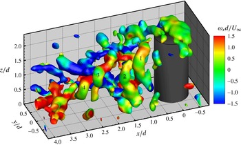
Instantaneous field (
 $t=13.6~\text{s}$
) with the isosurface of
 $Q/(U_{\infty }/d)^{2}=1.1$
coloured by
 $\unicode[STIX]{x1D714}_{x}d/U_{\infty }$
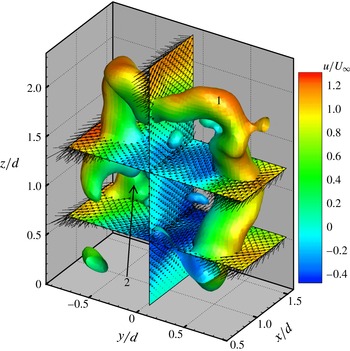
. The numbers are marked as the arch vortex or its fragments.


Substantial investigations (Fröhlich & Rodi Reference Fröhlich and Rodi2004; Pattenden et al.
Reference Pattenden, Turnock and Zhang2005; Frederich et al.
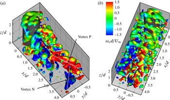
Reference Frederich, Wassen, Thiele, Jensch, Brede, Hüttmann, Leder, Tropea, Jakirlic, Heinemann, Henke and Hönlinger2008; Krajnović Reference Krajnović2011) indicated that the arch vortex existed only in the time-averaged flow, but not in the instantaneous flow field. However, instantaneous arch vortices are observed in the present experiment. As evident in figure 7, the complete instantaneous vortex structures around the finite cylinder are displayed with the
 $Q/(U_{\infty }/d)^{2}$
isosurface coloured by the streamwise vorticity
 $\unicode[STIX]{x1D714}_{x}d/U_{\infty }$
. It is indicated that the flow field studied here is complex and highly three-dimensional with various vortex structures. The vortex system on the free end occurs due to the flow separation at the leading edge. Evidently, the vortex cluster of the wake field slopes towards the bottom wall due to the downwash effect. An arch vortex with an M shape in the instantaneous field, similar to the one in the time-averaged flow field, is discernable and labelled 1 in figures 7 and 8. The legs of the instantaneous arch vortex incline in the streamwise direction, resulting from the separation on the cylinder sidewalls near the free end being delayed by interaction with the separated flow on the top. The inclination of the K–H vortex was also observed in the simulation results by Krajnović (Reference Krajnović2011). In addition, the separation over the free end is more upstream than that from the cylinder sides, as shown by the above mean vortex filaments in figure 6. It is interesting that the arch vortex labelled 1 is very similar to the model proposed by Wang & Zhou (Reference Wang and Zhou2009). It was demonstrated in their model that the bend upstream of the head (i.e. the horizontal part) resulted in a streamwise-component vorticity on the ‘shoulder’ of the arch structure, thus the tip vortex was a part of the arch vortex. Even so, as discussed above, the tip vortex is not the representation of the Karman vortex and simply blended with the arch vortex. Furthermore, it is more likely that the tip vortex is the transition between the shedding vortex from the sidewalls and the free end. It is actually indicated that the vertical and horizontal shedding vortex, corresponding to the legs and the head of the arch vortex, are connected by the tip vortex. Therefore, the explanation for the arch vortex in the present work is distinct from the one for the arch-type model proposed by Wang & Zhou (Reference Wang and Zhou2009). In addition, similar to the observation in the mean flow field, the sunken phenomenon of the horizontal part of the arch structure due to the downward motion is also observed in the instantaneous field. It should be mentioned that in figure 7, several quasi-streamwise vortices with opposite senses of rotation can be observed near the end of the measurement volume, which will be discussed in § 4.3.
It is noted that the integrated arch structure is not sustained for a long distance. On the contrary, the arch vortex dissipates and seems to be torn from the wake centreline by the downwash flow soon after its formation. As evident in figure 7, the vortex structures labelled 2, 3 and 4 are fragments of the arch vortex formed before the arch structure labelled 1. Precisely after the breakdown, the residue of the arch vortices can be a single-leg vortex (i.e. vertical vortex number 2) or a tilted hairpin-like vortex (number 3, 4). Then, all of them interact with the other structures in the wake and develop or dissipate downstream. Figure 8 shows an evident arch structure (number 1) extracted from figure 7. Three slices,
 $y/d=0$
and
 $z/d=0.55$
, 1.3, are extracted to display the details of this arch vortex. Generally, the shedding mode can be determined from the observation of the instantaneous fields. For a finite cylinder, there may exist both types of vortex shedding: antisymmetric Karman vortices and symmetric arch-type vortices (Sakamoto & Arie Reference Sakamoto and Arie1983; Sumner et al.
Reference Sumner, Heseltine and Dansereau2004; Palau-Salvador et al.
Reference Palau-Salvador, Stoesser, Fröhlich, Kappler and Rodi2010; Wang et al.
Reference Wang, Cao and Zhou2014a
). The simultaneous occurrence of the two shedding modes along the cylinder span is first observed in the present work. It is indicated in figure 8 that at this instant, the symmetrically arranged vortices occur in the upper part (
 $z/d=1.3$
) of the wake, while the antisymmetric arranged vortices occur in the lower part (
 $z/d<0.55$
). This leads to an imperfect arch vortex with one of the legs incomplete. The incomplete (or shorter) leg is located in
 $y/d<0$
, while the one in
 $y/d>0$
is longer and closer to the base. It can be concluded from the above observations that the reasons for the formation of the integrated arch vortex in the instantaneous field are as follows. First, the dominated downwash flow promotes the symmetric shedding (Wang et al.
Reference Wang, Zhou, Chan and Lam2006). Second, the symmetric shedding vortex from the sidewalls can be coupled with the separated vortex from the free end. Finally, the tip vortex connects the vertical and horizontal vortex.
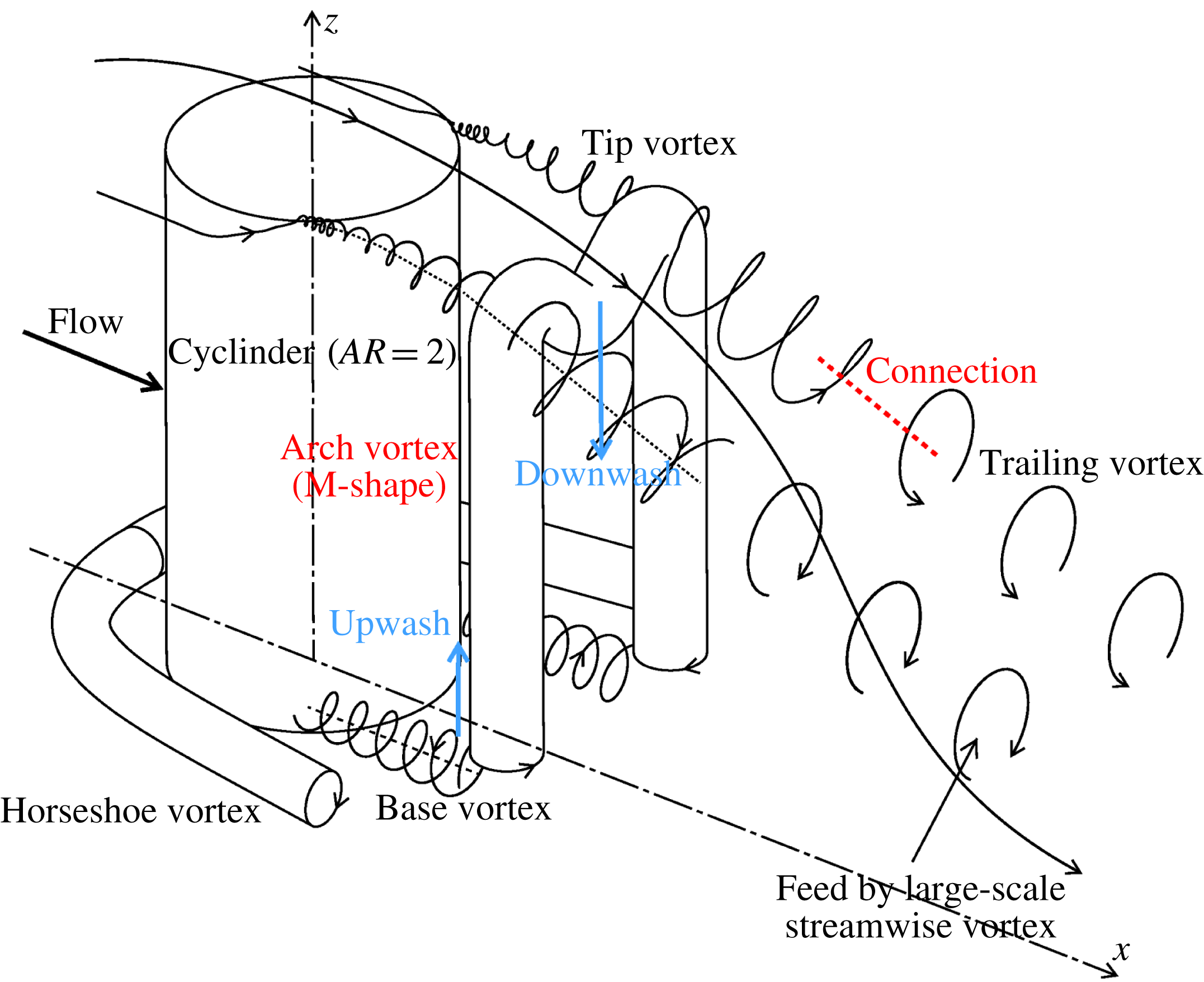
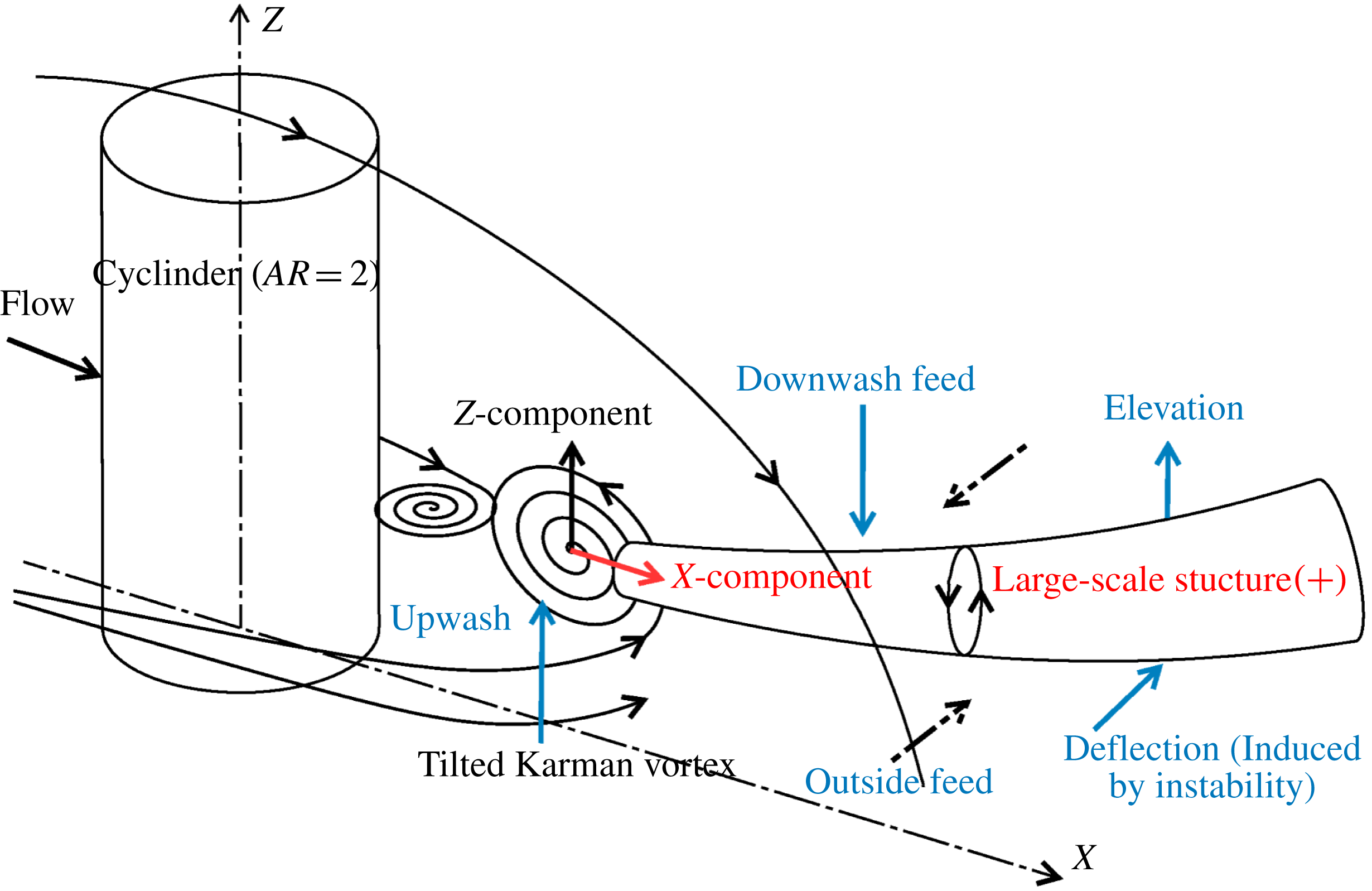
Sketch of the mean flow field around a finite circular cylinder for
 $AR=2$
.

Based on the analysis above, the typical structures and their details in the mean flow field are observed clearly, and the spatial locations and the coherent relations among these structures are determined. At this point, the complete characteristics of the mean wake field for the finite cylinder of
 $AR=2$
are obtained and sketched in figure 9. The mean tip, base, arch and trailing vortex and their locations and interactions are described in this sketch. It is noteworthy to point out that while the concepts of these typical structures have been proposed in the literature, their true three-dimensional configurations are first observed through the present experiment. Though there are various vortex structures in the sketch, we lay emphasis on the tip vortex and the arch vortex. In particular, the relation between the arch vortex and the tip vortex are clearly observed, i.e. the tip vortex is blended with the arch vortex, which could not be observed with the planar measurement in the previous experiments. In addition, it highlights that the connection between the tip vortex and the trailing vortex and the instantaneous M-shape arch vortex with its development are first found.
4.3 Large-scale streamwise vortex development
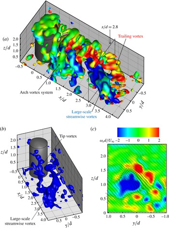
A strong large-scale streamwise vortex was first observed in the instantaneous three-dimensional wake fields. Figure 10(a) shows an instantaneous field with the isosurface of normalized
 $Q$
coloured by
 $x$
-vorticity. Again, the wake field presents the characteristics of three-dimensionality and complexity. Besides the arch vortex system, a single large-scale streamwise vortex with the negative sense of rotation is clearly observed in figure 10(a). The small-scale tip vortex and the large-scale streamwise vortex are presented in figure 10(b), which agrees fairly with the observation shown in figure 3. It is worth pointing out that the tip vortex near the free end is independent of the large-scale streamwise vortex. It is shown in figure 10(a,b) that the negative large-scale structure appears to escape from the ‘door’ of the arch vortex system. In other words, the large-scale streamwise vortex originates from the lower part of the wake and close to the cylinder. It means that this streamwise vortex is different from the tip vortex and trailing vortex discussed in § 4.1. From the observations of figures 3 and 10, it is indicated that subsequent large-scale streamwise structures with opposite senses of rotation are shed over time. That explains why this single streamwise vortex disappears in the time-averaged flow field, as shown in the sketch of figure 9. When extending downstream, the streamwise vortex deflects from the wake centreline to the positive
 $y$
-direction with a little uplift due to the wake instability. Figure 10(a) shows that the negative large-scale structure carries the positive streamwise vortex (i.e. the trailing vortex) and swings (or deflects) to the region
 $y/d>0$
. This swing makes the trailing vortex in
 $y/d>0$
disappear or merge into the large-scale streamwise vortex, which is more clearly seen in the slice at
 $x/d=2.8$
(see figure 10
c).
Instantaneous field at
 $t=0.6~\text{s}$
. (a) Isosurface of
 $Q/(U_{\infty }/d)^{2}=1.0$
coloured by the streamwise vorticity; (b) isosurface of
 $\unicode[STIX]{x1D714}_{x}d/U_{\infty }=-1.0$
; (c)
 $y$
–
 $z$
slice at
 $x/d=2.8$
overlapped by the velocity vectors. Note that the
 $y$
–
 $z$
slice and dimensionless
 $Q$
isosurface share the same colour bar.

It is noted that the deflection and uplift of this large-scale vortex structure make a contribution to the far-field mean streamwise vorticity shown in figures 4(b) and 9, and thus the circulation peak occurs at
 $x/d=3.35$
, as shown in figure 5(b). The contribution of the streamwise vortex to the far-field mean streamwise vorticity is consistent with the observation of the coherent half-loop structure by Bourgeois et al. (Reference Bourgeois, Sattari and Martinuzzi2011) and Hosseini et al. (Reference Hosseini, Bourgeois and Martinuzzi2013). Moreover, the present work suggests that this deflected large-scale streamwise vortex is not the only contribution to the far-field vorticity. The far-field streamwise vorticity (see the positive trailing vortex located in
 $y/d<0$
in figure 10(a,c) is found in the present instantaneous field. That verifies the mechanism, as mentioned in § 4.1, in which the far-field streamwise vorticity is generated from adequately strong shear between the downwash flow and the outside flow of the wake. Therefore, the mean far-field streamwise vorticity shown in figure 4(b) could come from the contribution of the trailing vortex pair. To sum up, it is suggested that the mean streamwise vorticity, extending from the trailing edge of the free end to the end of the measurement volume in figure 4(b), is fed by these three instantaneous vortex structures, i.e. the tip vortex, the trailing vortex and the deflected large-scale streamwise vortex. Therefore, the three peaks of the circulation occur at
 $x/d=1.2$
, 2.35 and 3.35 in figure 5(b), corresponding to the contribution of the three flow structures, respectively.
The phase-averaged half-loop shed mode for the square obstacle of
 $AR=4$
proposed by Bourgeois et al. (Reference Bourgeois, Sattari and Martinuzzi2011) was characterized by the principal core and the streamwise connector strand, and the latter was predominant. They considered that this streamwise structure was the three-dimensional deformation and evolution of the initially vertical vortices (i.e. the Karman vortex from the sidewalls of the square cylinder). To the best of the author’s knowledge, the asynchronously downstream convections of the two legs induced a skew stretching of the arch vortex, which triggered the formation of the half-loop shed structure (Bourgeois et al.
Reference Bourgeois, Sattari and Martinuzzi2011; Hosseini et al.
Reference Hosseini, Bourgeois and Martinuzzi2013). However, the present instantaneous results (see figure 10) appear without the half-loop structure. The vertical principal core is not observed in the instantaneous field. As evident in figure 10, in addition, the arch vortices and the large-scale streamwise structures are spatially separated and have different scales, indicating that the arch vortex and the streamwise vortex are not likely to be contained in an integrated structure. The arch vortex disintegrates soon after its formation, as shown in figure 7. These inconsistencies are likely to be attributed to the inherent differences of the wake behaviour behind the square and circular cylinder, as mentioned above. For example, the formation mechanism of the tip vortex is different for the two cylinder cases, as discussed in § 4.1. The separation point (the side edges) is fixed for the square case while it is not for the circular case. Moreover, the relatively lower aspect ratio and thick turbulent boundary layer in the present investigation are the other critical reasons for the inconsistencies. Though the reason for the formation of this large-scale vortex structures is not clear here, one could conjecture that it may connect with the development of alternating spanwise shedding vortices in the lower wake region (see figure 10
a,b).
As shown in figure 10(b), the large-scale streamwise vortex starts at the cylinder sidewall near wall and becomes larger in size when extending downstream. On the other hand, the downwash flow from the free end and the upwash flow from the ground may change the direction of the vortex axis, which is considered as the three-dimensional deformation and stretching of the vortex structure. Further analysis will be conducted with a decomposition method in the next section.
5 POD analysis on the whole wake field
Proper orthogonal decomposition (POD) is a shared method to extract high energetic modes from the complex flow patterns (see Chatterjee Reference Chatterjee2000, for example). This method has been widely employed (Feng, Wang & Pan Reference Feng, Wang and Pan2011; He et al.
Reference He, Pan, Feng, Gao and Wang2016; Wang et al.
Reference Wang, Gao, Wei, Li and Wang2016b
). POD eigenvalues
 $\unicode[STIX]{x1D706}_{n}$
, sorted in the decreasing order, represent the energy of each mode. The mode temporal coefficients
 $a_{n}$
for each snapshot can be obtained by projecting the original velocity fields onto the POD modes. These coefficients describe the time-sequential energy fluctuation of the corresponding modes. With the statistical theory, the spectrum analysis can be performed on the time-varying coefficients to obtain their periodic properties. Generally, in the shedding process the wake behind the bluff body contains several periodic terms which represent the most energetic structures, and with these terms the original flow field can be reconstructed into a low-order flow model. Specifically, with the phase-angle detection, POD-based phase averaging can be conducted to reconstruct the flow field and judge the dynamic behaviour of the flow.
5.1 POD coefficients and spectrum analysis
In this paper, POD was applied to extract the three-dimensional periodical structures from the turbulent wake field behind the finite circular cylinder. The POD analysis was performed on the five separated datasets (1000 snapshots in total) of the time-sequential volumetric velocity fields to obtain their common spatial modes. Specially, the five datasets were put together in a time sequence before the traditional POD process. Before the application of POD, the time-averaged velocity is subtracted from each velocity signal.
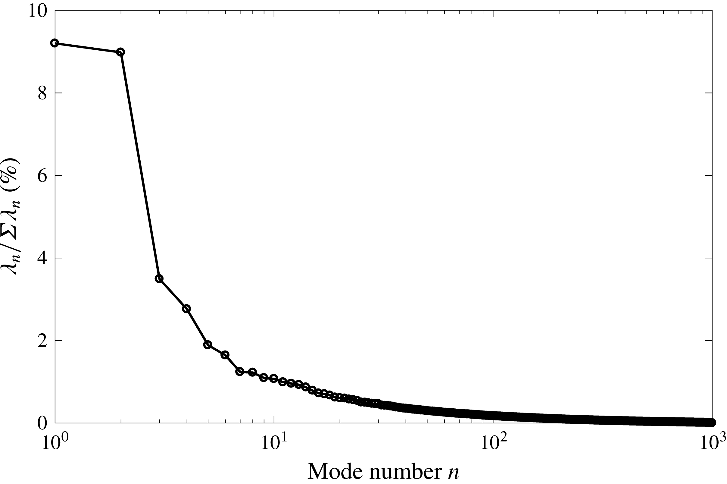
Energy percentages of the different POD modes.

The POD temporal coefficients
 $a_{n}$
will be normalized by their corresponding eigenvalues
 $\unicode[STIX]{x1D706}_{n}$
, i.e.
 $a_{n}^{\ast }=a_{n}$
(van Oudheusden et al.
Reference van Oudheusden, Scarano, Hinsberg and Watt2005; Wang et al.
Reference Wang, Cao and Zhou2014a
). The energy distributions (
 $\unicode[STIX]{x1D706}_{n}/\sum \unicode[STIX]{x1D706}_{n}$
) for all POD modes are plotted in figure 11. It is indicated that there exists a rapid decline in energy with increasing mode number, especially for the first several modes. This situation is valid and expected in POD modal analysis. The energy distributions of the first two modes are found to be similar and significantly larger than the other modes, which is the same result as observed in the case of the flow around an infinite cylinder. It is noteworthy to mention that the absolute energy content of the first modes is low, which might lead to the unsuccessful application of the POD technique. However, it is not the absolute energy content but the predominance of the first modes that plays a key role in the POD analysis. The first two modes (
 ${\approx}$
9 %) occupied approximately three times the energy of mode 3 (
 ${\approx}$
3.4 %) and mode 4 (
 ${\approx}$
2.6 %), and more than four times the energy of the other modes (
 ${\leqslant}$
2 %). On the other hand, the wake behind the finite cylinder immersed in the turbulent boundary layer is highly unsteady three-dimensionally, so it is predictable that the first modes have a lower energy compared with the infinite-cylinder cases. Nevertheless, the low energy content of the first modes does not impact determination of the periodic feature, as the results show below.
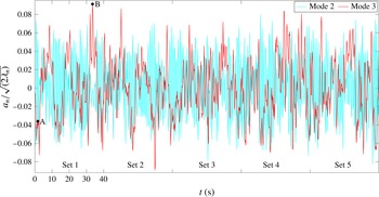
The POD coefficients of modes 2 and 3 for the five datasets. The letters A and B are located at
 $t=1.8$
and 33.6 s, respectively.

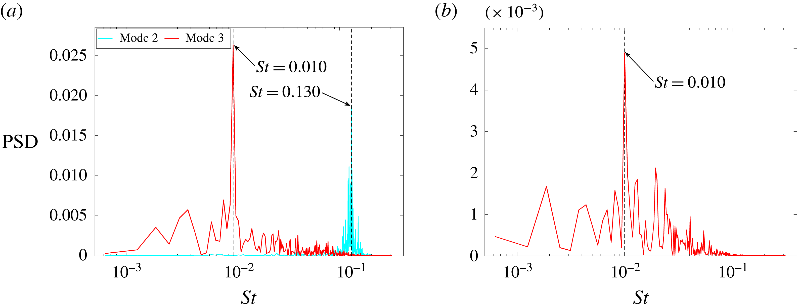
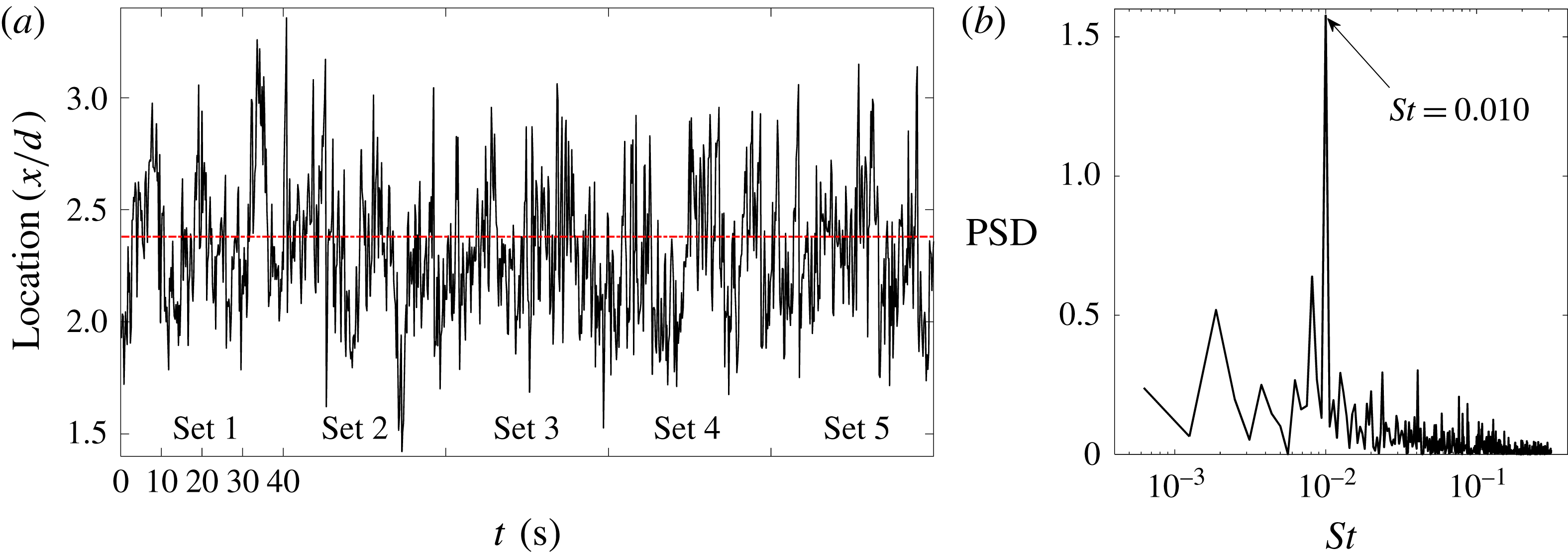
The corresponding power spectral density (PSD) functions of (a) modes 2 and 3 and (b) the envelope of mode 2.

Figure 12 displays the POD coefficients of modes 2 and 3 – mode 1 and mode 4 are not shown for clearer observation. The first two modes have a temporal phase shift of approximately
 $90^{\circ }$
. In addition, the temporal coefficients of mode 3 and mode 4 both show a relatively low frequency. In order to analyse the periodic features of these four modes, the power spectra are presented in figure 13. The ordinate represents the power spectral density (PSD) functions, defined as
 $|F|^{2}/(N\cdot Fs)$
, with
 $F$
the Fourier coefficients,
 $N$
the sample size and
 $Fs$
the sampling frequency. The ordinate scale is arbitrary for the spectrum analysis in figure 13, though the same scale is used for every spectrum for the purpose of comparison. As shown in the figures, the first two modes present clearly periodic characteristics and share the same peak at a Strouhal number (
 $St$
) of 0.130 (
 $\pm$
0.001), which is calculated by
 $St=fd/U_{\infty }$
(
 $f=1.038~\text{Hz}$
). A peak representing the low frequency (
 $St=0.010\pm 0.001$
) is evident for mode 3 shown in figure 13(a). It should be noted that modes 3 and 4 do not show a regular feature in the flow around the infinite (or 2D) cylinder without control (Feng et al.
Reference Feng, Wang and Pan2011), which indicates an underlying new phenomenon in the present experiment. The envelope for the temporal coefficients of mode 2 is extracted, which is formed by connecting the local maximum points of the temporal coefficients with splines. It is interesting that the same peak at
 $St=0.010$
in the power spectrum analysis of this envelope is presented in figure 13(b), which verifies the relation between the first pair and the second pair of modes. In the present work, mode 1 (or 2) and mode 3 (or 4) represent the two different wake topologies: antisymmetrically and symmetrically arranged vortex (shown later). To some extent, there exists a modulating effect of the second mode pair on the first mode pair according to the result of the enveloping line. It appears that this modulating motion causes a transformation of the different wake behaviours. Further discussion will be provided in § 5.3.
5.2 Origin and development of large-scale streamwise vortex
In order to determine the origin of the periodical features, the fast Fourier transform (FFT) method is separately performed on time series of the velocity at every measurement point in the whole wake field. This method, called Fourier mode decomposition (FMD), was proposed by (Ma et al.
Reference Ma, Feng, Pan, Gao and Wang2015). The FMD method is based on the application of the discrete Fourier transform (DFT) at each spatial position. The amplitude of the Fourier mode represents the fluctuation statistics (i.e. energy) of every sampling point corresponding to the eigen-frequency of interest. It could be regarded as a way to decompose the flow history into two parts: the mean flow and a series of modes with the simple harmonic fluctuations. Thus, this method can effectively decompose the global flow into individual characteristic frequencies and assist in finding the origin of the periodic features, which is elaborated by Ma et al. (Reference Ma, Feng, Pan, Gao and Wang2015). With this method, the fluctuation energy of the
 $x$
-component velocity corresponding to the normalized eigen-frequency
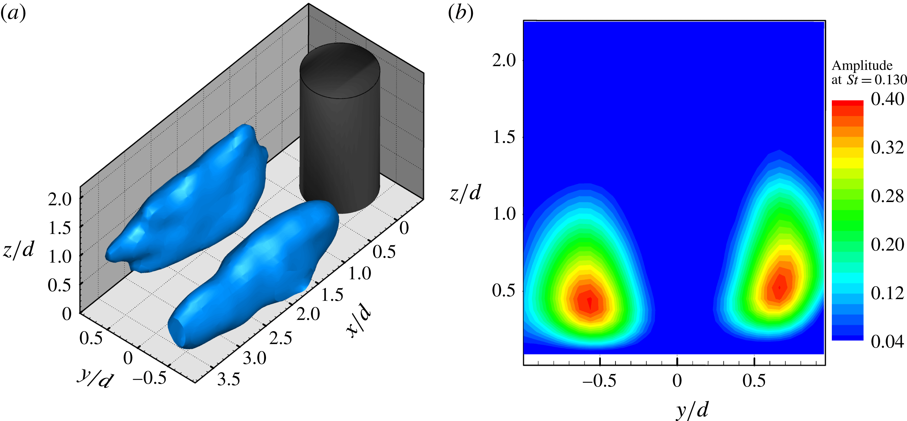
 $St=0.130$
is extracted for every point. The amplitude isosurface of velocity fluctuation at every point is displayed in figure 14. Similar to the configuration of the infinite cylinder, the high-amplitude region is distributed on both sides of the wake.
The result of FMD: the isosurface (a) and the extracted slice (b) at
 $x/d=1.75$
of the fluctuation energy corresponding to an eigen-frequency of
 $St=0.130$
. A high 3D-contour value occurs on both sides in the lower part of the cylinder wake.

Dimensionless
 $Q$
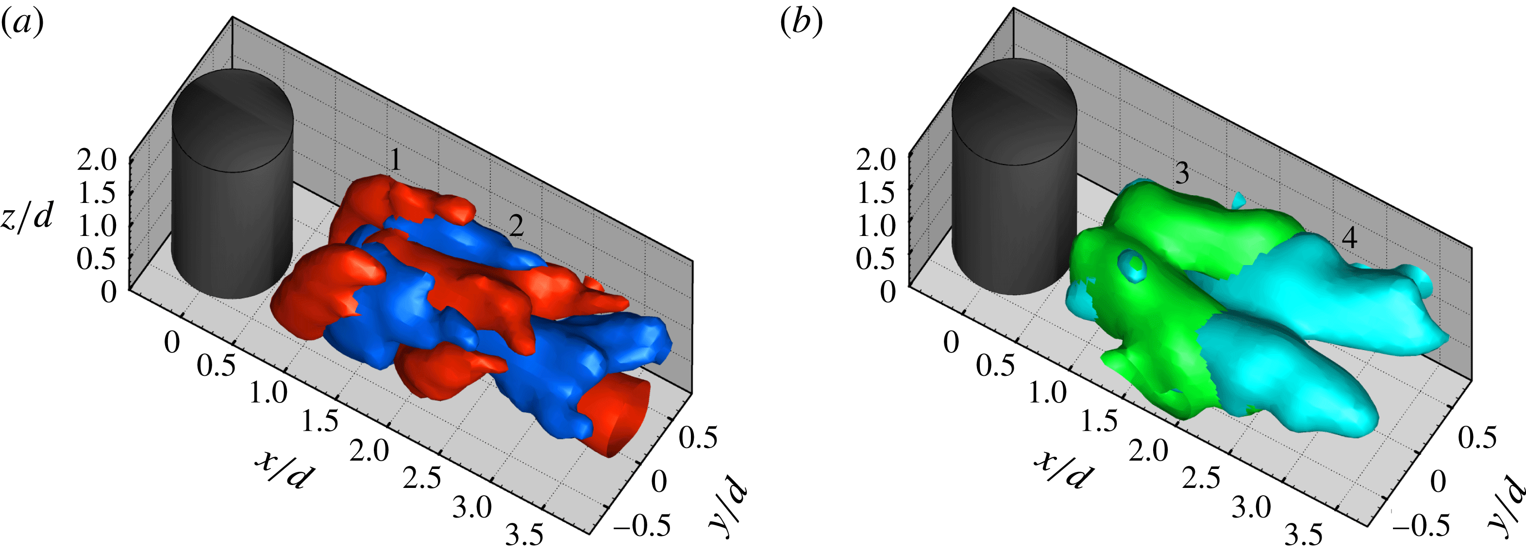
isosurface of the first four POD modes: (a) the first pair of modes, (b) the second pair of modes. Note that the colour does not denote the sense of vortex rotation, but distinguishes between the different modes. These modes are marked by the corresponding numbers.

Moreover, it is found in figure 14(b) that the high-contour value occurs in the lower part of the cylinder wake, which means that the shedding signal in the lower part is more evident than the one in the upper part. This amplitude distribution derived from FMD confirms that the peak of vortex-shedding signal tends to be ill-defined near the top and becomes apparent away from the top (Sumner et al. Reference Sumner, Heseltine and Dansereau2004; Adaramola et al. Reference Adaramola, Akinlade, Sumner, Bergstrom and Schenstead2006).
In addition, to clarify the flow features of the POD modes, the
 $Q$
isosurfaces are obtained based on the POD-reconstructed velocity field with the corresponding modes. Figure 15 presents the first four POD modes with dimensionless
 $Q$
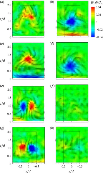
isosurfaces. It is shown that the first pair of modes is characterized by the alternating streamwise vortex, which is shown more clearly in figure 16. The slices (figure 16
a–d) at the different streamwise locations for modes 1 and 2 display the in-plane vorticity and velocity vectors. These figures indicate that the positive and negative streamwise vortices convect up and down alternatingly in the
 $x$
-direction, similar to the features of the Karman vortex. In the present work, for example, Karman vortex sheds left and right alternatingly in the
 $x$
–
 $y$
plane. Besides, the vortex structures near the free end disappear in the first two modes, and thus it suggests that the tip vortex is not the representation of the Karman vortex. The other evidence that the tip vortex is independent of the spanwise vortex is provided with the discussion of figures 2, 6 and 14. As discussed above, the same peak at
 $St=0.130$
is found for the spectrum analysis of the first two modes. It is conjectured that an underlying relation exists between the formation of the large-scale streamwise structure and alternating vortex shedding from the lower-part cylinder sidewalls. In order to confirm this relation and the periodic features corresponding to the first two modes, the phase-averaging method was performed. It has been shown that the first two temporal coefficients pertaining to a periodic wake flow can be used to identify the phase of the dominant coherent structures (van Oudheusden et al.
Reference van Oudheusden, Scarano, Hinsberg and Watt2005). The phase angle at every snapshot is estimated by
 $\unicode[STIX]{x1D703}=\arctan [a_{2}(t)/a_{1}(t)]$
, where
 $a_{1}$
and
 $a_{2}$
are the normalized temporal coefficients (shown in figure 12) of the first two modes. After determining the phase of every snapshot, the instantaneous velocity field can be phase-sorted to obtain the phase-averaged representations of the periodic vortex shedding. For more details about the phase average technique refer to van Oudheusden et al. (Reference van Oudheusden, Scarano, Hinsberg and Watt2005). Based on the analysis above, a phase bin size of
 $36^{\circ }$
was considered in the present investigation. Then all data that fell into the same bin were averaged. It resulted in 10 distinct phases (
 $0^{\circ }$
,
 $36^{\circ }$
,
 $72^{\circ },\ldots$
) in one cycle being obtained to give a picture of the periodicity in the wake field. As a consequence, a low-dimensional representation of the wake field was acquired by reconstruction with the first pair of modes.
The extracted slices from the first four POD modes are contoured by the streamwise vorticity with the overlapped vector fields. First row for mode 1: (a)
 $x/d=1.6$
, (b)
 $x/d=3.2$
; second row for mode 2: (c)
 $x/d=2.4$
, (d)
 $x/d=3.9$
; third row for mode 3: (e)
 $x/d=1.5$
, (f)
 $x/d=3.5$
; fourth row for mode 4: (g)
 $x/d=2.8$
, (h)
 $x/d=3.9$
.

Reconstructed flow fields in the phase-averaged results based on the first pair of modes for phases
 $PN=2$
(a) and
 $PN=7$
(b). Isosurface of
 $Q/(U_{\infty }/d)^{2}=1.0$
is coloured by
 $x$
-vorticity.

In-plane velocity vectors, streamlines and
 $z$
-vorticity fields in the phase-averaged results at the slice
 $z/d=0.35$
for phases
 $PN=2$
(a) and 7 (b).

Sketch for the formation and development mechanism of the instantaneous large-scale streamwise structure.

Figure 17 presents two typical snapshots of the reconstructed flow field from the phase-averaged results. Their phase numbers (
 $PN$
) are 2 and 7, which represents phase angles of
 $36^{\circ }$
and
 $216^{\circ }$
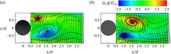
, respectively. It is shown that the long streamwise vortex convects downstream and deflects from the wake centreline. As evident in these two snapshots, a ‘small’ structure is located below the ‘large’ streamwise structures with the opposite sense of rotation to the small one, and these two structures have opposite directions of extension. In other words, subsequent large-scale structures with the opposite sense of rotation are shed alternatingly. The phase-averaging analysis reveals that the periodic characteristic of the wake field is reflected by the alternating large-scale streamwise structure. It is also found that the finite-cylinder wake is dominated by the alternating streamwise structure as well as the arch vortex shown in figure 17. In addition, figure 18 shows the velocity vectors and the associated in-plane wall-normal vorticity overlapped by streamlines at
 $z/d=0.35$
for
 $PN=2$
and 7. It is indicated that the flow patterns are typical of the Karman vortex (i.e. antisymmetrical vortex) shedding at the distinct phases. Combined with the FMD result, it is verified that the large-scale streamwise vortex is connected with the antisymmetrically shedding vortex from the lower part of the cylinder. Precisely, the large-scale streamwise structure originates from the lower-part vertical Karman vortex. This reoriented-vortex mechanism, i.e. the vertical vortex deforms to the streamwise vortex, is consistent with the streamwise connector in the half-loop model proposed by Bourgeois et al. (Reference Bourgeois, Sattari and Martinuzzi2011). Based on the analysis above, the formation mechanism of this long streamwise vortex can be determined. With the upwash effect near the wall, the Karman vortex on one side at lower heights of cylinder is uplifted and inclines towards the
 $x$
-direction. As a consequence, this tilted vortex has an
 $x$
-component vorticity. Extending downstream, this streamwise-component vortex is enhanced by highly three-dimensional stretching and deformation. In addition, this streamwise vortex is fed by the upwash/downwash and the outside flow, which makes it stronger. On the other hand, the dispersed fragments of the arch vortex and the trailing vortex (see figures 7 and 10) merge into and strengthen the large-scale structures. Under the arch vortex system, this strong streamwise vortex continues to extend downstream with a little uplift. Because of the alternating shedding effect, the long streamwise vortices are shed alternatingly and wiggle when convecting downstream. Figure 19 displays a simplified sketch of the formation and development of this large-scale streamwise structure.
5.3 Low-frequency symmetric-topology mode
5.3.1 2D/3D symmetric wake topology
The four slices at
 $z/d=0.35$
contoured by the wall-normal vorticity with the overlapped vector fields, which are extracted from mode 1 (a), mode 2 (b), mode 3 (c) and mode 4 (d), respectively.

Instantaneous dimensionless
 $Q$
fields coloured by the streamwise vorticity corresponding to point A (a) and point B (b) shown in figure 12.

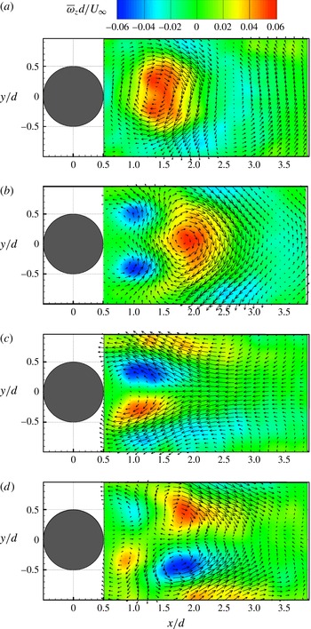
In figure 20, the four slices at
 $z/d=0.35$
contoured by the wall-normal vorticity with the overlapped vector fields are extracted from the first four modes. It is indicated that mode 1 and mode 2 represent an antisymmetric arranged pattern, similar to the infinite-cylinder cases, while mode 3 and mode 4 represent an evidently symmetric arranged pattern. In figure 20(a,b) the vorticity concentrations seems to be stretched laterally compared with the infinite-cylinder cases. This phenomenon is attributed to the downwash effect from the free end (Wang et al.
Reference Wang, Cao and Zhou2014a
). This downward motion acts to entrain fluid near the free end and to separate the shear layers separated from the cylinder sidewalls, resulting in widening the near wake. In figure 15(b), modes 3 and 4 represent a pair of streamwise vortex with opposite sense of rotation, which shows a relatively 3D symmetric wake topology compared to the first pair of modes. This observation is more clearly seen from the 2D symmetrical vortex configuration shown in figures 16(e,g) and 20(c,d). Surprisingly, the observations on the extracted
 $y$
–
 $z$
slices in figure 16 and
 $x$
–
 $y$
slices in figure 20 further suggest that the streamwise vortex (
 $x$
-direction) in the lower part of the cylinder is intimately connected with the spanwise vortex (
 $z$
-direction) shedding from the cylinder sidewalls (see figure 19).
The symmetric shedding mode can also be determined from the direct observation of the 3D instantaneous wake fields, as shown in figures 7 and 21. In figure 12, the point B in the profile of the POD coefficients indicates that the coefficients of mode 3 reach peaks while the coefficients of mode 1 and 2 fall and tend simultaneously to zero. It is found that large
 $a_{1}$
and
 $a_{2}$
correspond to antisymmetrical vortex shedding, while the small values lead to symmetrical vortex shedding (Wang et al.
Reference Wang, Cao and Zhou2014a
). The small temporal coefficients of the first two modes (
 $a_{1}$
,
 $a_{2}$
) or the large coefficients of mode 3 correspond to the 3D symmetric wake behaviour in the present work. In figure 21, the instantaneous flow fields corresponding to the points A (
 $t=1.8~\text{s}$
) and B (
 $t=33.6~\text{s}$
) in figure 12 are displayed with the dimensionless
 $Q$
isosurface coloured by
 $x$
-vorticity. The instantaneous flow field at point A shows two deflecting streamwise vortices P and N. Vortex P (marked with polygonal line) occurs close to the cylinder and the relatively small-scale vortex N (marked with white dotted line) is located below P, which presents the feature of antisymmetry and alternating convection. Similar observations, positive and negative large-scale streamwise structure, are also presented in figures 3 and 10, respectively. Unlike point A, the wake field at point B does not show a long deflecting streamwise vortex but a relatively symmetrical characteristic. It seems that the large-scale streamwise vortex breaks down in the arch vortex system. A similar configuration of the flow field in figure 21(b) is also observed at other points with the same features of temporal coefficients as point B. We attempt to explain this 3D symmetric wake behaviour such that the low aspect ratio is one of the critical reasons. In the current work, the cylinder is relatively short, thus the downwash flow can extend over most of the height of the cylinder and trigger the symmetric shedding vortex, which was elaborated in the previous sections. In this regard, symmetric wake behaviour is not likely to be observed for the tall cylinder of
 $AR>3$
(Wang & Zhou Reference Wang and Zhou2009; Bourgeois, Noack & Martinuzzi Reference Bourgeois, Noack and Martinuzzi2013). The other reason for the 3D symmetric wake could be breakdown of the large-scale streamwise vortex due to suppression by whole movement of the separated shear layers. The characteristics of the instantaneous flow fields have closely corresponding connections with the amplitude of the temporal coefficients, as shown in figures 12 and 21. Therefore, the probability of occurrence of a flow structure may be determined from the distribution of the POD coefficients (Wang et al.
Reference Wang, Cao and Zhou2014a
). To sum up, based on analysis of the temporal coefficients in figure 12, a quantification of antisymmetric and symmetric types of wake behaviour has been made in the present work.
It may be surprising that modes 3 and 4 both show the symmetric arranged vortex in figures 16(e,g) and 20(c,d) in the present experiment because mode 4 generally shows a different feature from mode 3 in previous studies on the flow around the cylinder without control (Feng et al.
Reference Feng, Wang and Pan2011; Wang et al.
Reference Wang, Cao and Zhou2014a
; Qu et al.
Reference Qu, Wang, Sun, Feng, Pan, Gao and He2017). It should be mentioned that the symmetry property in flow around a finite-square cylinder was also studied by Bourgeois et al. (Reference Bourgeois, Noack and Martinuzzi2013). They obtained harmonic modes that are extracted from a POD expansion of the symmetric and antisymmetric components of the velocity fluctuation, while in the present experiment, POD analysis is directly performed on the velocity fluctuation. Mode 3 from the traditional linear POD is not an isolated mode so this mode does not represent the shift mode which is obtained through the nonlinear interaction terms (Noack et al.
Reference Noack, Afanasiev, Morzyński, Tadmor and Thiele2003; Tadmor et al.
Reference Tadmor, Lehmann, Noack and Morzyński2010; Bourgeois et al.
Reference Bourgeois, Noack and Martinuzzi2013). In addition, earlier observations (Sattari, Bourgeois & Martinuzzi Reference Sattari, Bourgeois and Martinuzzi2012; Wang et al.
Reference Wang, Cao and Zhou2014a
) are reconciled showing that the symmetric shedding of vortices is a rare or random occurrence. It means that the existence of the symmetric wake behaviour without flow control cannot show a regular feature with a certain frequency due to the inherent instability. In the present experiment, however, the second pair of modes is characterized by regularly symmetric shedding with a low frequency of
 $St=0.010$
(see figures 12 and 13). Therefore, there may exist an underlying mechanism used to explain this new phenomenon, and in this work this mechanism is considered to be the low-frequency flapping phenomenon observed in the backward-facing step flow, which is discussed below.
The slices at
 $y/d=0$
extracted from the corresponding instantaneous flow fields in figure 21. The points
 $\text{S}_{A}$
and
 $\text{S}_{B}$
indicate the closure of the recirculation zone.

Reattachment location fluctuation (a) and corresponding power spectrum (b) at the slice
 $y/d=0$
. The red dashed line in (a) indicates the mean reattachment location
 $x/d=2.38$
.

5.3.2 Flapping phenomenon and its effect on the wake behaviours
Figure 22 shows slices at
 $y/d=0$
extracted from the two flow fields in figure 21; the in-plane instantaneous vectors and streamlines show reversed flow behind the cylinder. Evidently, the shapes of the lee recirculation zone are different in these two instantaneous flow fields. The length of the recirculation zone for the symmetric wake (see the point
 $\text{S}_{B}$
in figure 22
b) is much longer than the one for the antisymmetric wake (see the point
 $\text{S}_{A}$
in figure 22
a). Observations on the length of the recirculation zone were also conducted by previous investigations (Bourgeois et al.
Reference Bourgeois, Noack and Martinuzzi2013; Wang et al.
Reference Wang, Cao and Zhou2014a
). In the present study, the longer recirculation length corresponds to the symmetric topology of the wake and the disappearance of the large-scale streamwise vortex (see figure 21
b). More precisely, the recirculation length seems to be linked to the strength of the upwash flow from the wall. In figure 22, the upwash flow for the antisymmetric configuration is stronger than that for the symmetric configuration. That is understandable, as the upwash flow triggers the formation of large-scale streamwise structures (see figure 19). On the other hand, the longer recirculation zone means that the separated shear layer from the cylinder sidewalls and the free end extend more downstream and restrain the deflection or even formation of the long streamwise vortex. Consequently, this restraining makes the wake field symmetric, as observed in the instantaneous field at point B. The comprehensive analysis of the POD modes and the instantaneous flow fields reveals the intermittence in the finite-cylinder wake.
We attempt to explain the cause of formation of the low-frequency symmetric-topology mode. As discussed above, this 3D symmetric wake behaviour is ascribed to the effect of low aspect ratio and the extension of the separated shear layer in the present work based on the previous investigation, this type of long period (i.e. low-frequency) flow appears to originate from the flapping of the recirculation zone. The flapping phenomenon is common knowledge in the flow over a backward-facing step (Eaton & Johnston Reference Eaton and Johnston1980; Friedrich & Arnal Reference Friedrich and Arnal1990; Le, Moin & Kim Reference Le, Moin and Kim1997; Schäfer, Breuer & Durst Reference Schäfer, Breuer and Durst2009). As elaborated in the literature, the backward-facing step flow is prone to oscillations of the reattachment length of the primary recirculation region, also denoted ‘flapping’. The present work considers fluctuation of the reattachment point as the representation of flapping. In order to reveal this low-frequency flapping, the instantaneous streamwise location of the reattachment point at the slice
 $y/d=0$
is measured. The mean streamwise position is at
 $x/d=2.38$
, as shown in figure 2(c). Figure 23 shows fluctuation of the location of the reattachment point and its energy spectrum. It might be surprising that the feature of time-sequential reattachment locations is very similar to that of the temporal coefficients for mode 3 (see figures 12 and 23
a), and these two time series share the same peak in their power spectrum (see figures 13
a and 23
b). Therefore, there is oscillation of the reattachment point so that the whole recirculation zone represents the low-frequency action of the wake. That is, the low-frequency oscillation of the wake field and the antisymmetric spanwise vortex coexist and this flapping phenomenon has an effect on the different wake behaviours for the finite-cylinder wake. Therefore, the antisymmetric wake behaviour occurs most of the time and the symmetric one occurs intermittently.
6 Conclusions
The present study investigates the time-averaged and instantaneous three-dimensional flow structures in the wake field behind a finite circular cylinder with an aspect ratio of 2. The short cylinder is mounted on the bottom of the water tunnel and immersed in the turbulent boundary layer. Tomographic particle image velocimetry with six high-resolution CCD cameras is applied to conduct this measurement, and is successful in the description of the vortex-dominated wake flow behaviour.
Some novel results are obtained in this work. The mean streamwise vortex is of a dipole type in which a pair of streamwise vortices (i.e. the tip vortex) originates from the trailing edge of the free end and connects the trailing vortex near the reattachment zone. The relatively thick boundary layer triggers the formation of a weak base vortex at the rear wall junction. The arch vortex behind the cylinder is found to be a typical flow structure not only in the time-averaged field, as observed in the previous studies, but also in the instantaneous field. The mean arch vortex (
 $Q$
isosurface) shows an M shape instead of a reversed U shape due to the existence of the tip vortex and associated downwash effect. Based on the characteristics of these mean vortex structures, a refined sketch of the mean wake field for the finite cylinder of
 $AR=2$
is presented in figure 9.
A full picture of the instantaneous flow field behind the finite cylinder of
 $AR=2$
is first captured in the present experiment. The instantaneous wake fields are highly unsteady three-dimensionally and involve many novel phenomena. The spatial positions of the typical structures and their relations are clearly observed. The tip vortex is blended with the arch vortex. Precisely, in the instantaneous arch vortex, the tip vortex connects the horizontal vortex from the free end to the vertical vortex from the sidewalls. The development of the arch vortex is also discussed. Remarkable is the observation of the large-scale streamwise vortex which forms in the lower part of the cylinder (i.e. below the arch vortex system). Consequently, the instantaneous wake flow field is dominated by the arch vortex system and the long streamwise vortices. The large-scale streamwise vortex, originating from the deformation of the lower-part Karman vortex, deflects to one side and devours the trailing vortex and the fragments of the arch vortex on this side. Thus, it can be concluded that the mean streamwise vorticity comes from the contributions of the tip vortex, trailing vortex and the deflected large-scale streamwise vortex. Due to wake instability, this single large-scale vortex with a different sense of rotation at different instants swings alternatingly, which makes the wake antisymmetric. The formation and development of this instantaneous large-scale streamwise structure are sketched in figure 19.
The discussion of the 2D/3D symmetric wake behaviour is first provided with the observations on the POD modes and the instantaneous flow fields in the present work. The first pair of POD modes shows an antisymmetric arranged vortex while the second pair shows a symmetric arranged vortex. The extracted
 $x$
–
 $y$
and
 $y$
–
 $z$
slices (figures 16 and 20) from the first four modes suggest that the large-scale streamwise vortex in the lower part of the cylinder is intimately connected with the spanwise vortex shedding from the cylinder sidewalls, which is confirmed in the phase-averaged results. The instantaneous three-dimensional symmetric wake behaviour is first experimentally observed with TPIV in the present study. It is attributed to the short-cylinder effect due to dominant downwash flow promoting symmetric shedding and the extension of separated shear layers which suppress the evolution of the large-scale streamwise vortex. For that reason, the symmetric wake is not likely to occur for tall cylinders (
 $AR>3$
). In addition, the characteristics of the instantaneous flow fields have closely corresponding connections with the amplitude of the temporal coefficients, which corroborates that the probability of occurrence of a flow structure could be determined from the distribution of the POD coefficients. Therefore, qualification and quantification of antisymmetric and symmetric types of wake behaviour have been made with the POD method in the present work.
When an antisymmetric spanwise vortex or large-scale streamwise vortex occurred, the whole wake field flapped (or oscillated) simultaneously. The low-frequency feature is due to the flapping phenomenon observed in the backward-facing step flow. This flapping phenomenon of the recirculation zone, which is determined by measuring the recirculation length, has an impact on the three-dimensional wake behaviour. It is found that the longest recirculation length corresponds to a symmetric topology of the wake and the disappearance of the large-scale streamwise vortex (see figures 21 and 22). In addition, the recirculation length seems to be linked to the strength of the upwash flow from the wall. The longer recirculation zone indicates that the separated shear layer from the cylinder sides and the free end extends more downstream and restrains the deflection or even the formation of the long streamwise vortex. Consequently, this restraining makes the wake symmetric. It is worth mentioning that for the flow around an infinite cylinder without control, the third and fourth POD modes do not show regularly symmetric shedding, in contrast to the present results. It means that there exists an underlying auto-flow-control mechanism in the flow around the short cylinder. Though the appearance of the antisymmetric type is more frequent than the symmetric type, the capture of the low-frequency mode is of significance in practical applications.
Although the above phenomena are observed under the current conditions (
 $AR=2$
,
 $\unicode[STIX]{x1D6FF}/h=1.025$
), it could be conjectured reasonably that these phenomena also occur for flow over small-aspect-ratio obstacles immersed in a thick boundary layer. Direct observations and statistical analysis on the three-dimensional instantaneous flow field enhance the understanding of the complex separated flow and have some guiding significance for flow control. In short, the present results fill gaps in the related field and make a contribution to studies on the flow over obstacles with respect to the flow-induced noise and drag reduction. It should also be mentioned here that the sampling frequency is low in this investigation, which means that the time resolution is not high enough, and the transformation between symmetric and antisymmetric wake behaviours has not been identified, and needs further studies.
Acknowledgements
This work was supported by the National Natural Science Foundation of China (grant nos. 11327202 and 11490552).