1 Introduction
The high-frequency load and response experienced by a monopile exposed to ocean waves are of interest for the renewable industry, where the cylindrical monopile is by far the most popular support structure for wind turbines. With a focus on cost reduction and more optimized design, the industry is seeking improved understanding of the nonlinear wave load mechanisms that are driving high-frequency resonance responses (Zhen et al. Reference Zhen, Bingham and Nicholls-Lee2015).
The linear wave load, as found for a vertical cylinder by MacCamy & Fuchs (Reference MacCamy and Fuchs1954), is well defined. Also adequately covered are the nonlinear harmonic forces at
 $2\unicode[STIX]{x1D714}$
and
 $3\unicode[STIX]{x1D714}$
, where
 $\unicode[STIX]{x1D714}$
is the fundamental wave frequency. These harmonic forces have been the focus of several previous works. For regular waves, the second harmonic force has been analysed by Taylor & Hung (Reference Taylor and Hung1987), Chau & Eatock Taylor (Reference Chau and Eatock Taylor1992) and Newman (Reference Newman1996b
), while the third harmonic force has been analysed by Faltinsen, Newman & Vinje (Reference Faltinsen, Newman and Vinje1995) and Malenica & Molin (Reference Malenica and Molin1995). The latter method by Faltinsen, Newman & Vinje, referred to as FNV, is a long-wave approximation for deep water. This was later extended to the case of irregular waves by Newman (Reference Newman, Grue, Gjevik and Weber1996
a
). Recently, Kristiansen & Faltinsen (Reference Kristiansen and Faltinsen2017) have generalized FNV to finite water depth. For regular waves of moderate wave slope, the theoretical results show good agreement with measurements, while for steeper waves, a discrepancy is observed, indicating important shortcomings in the modelled
 $3\unicode[STIX]{x1D714}$
force.
The present work investigates the remaining part of the forces, i.e. the force contribution above
 $3\unicode[STIX]{x1D714}$
, where more work is needed, particularly for steep waves. This nonlinear force contribution has two main peaks in the time domain. The first peak occurs when the wave crest hits the cylinder, when the total load is positive. The second peak occurs between the passage of the wave crest and the following trough, close in time to the zero downcrossing of the wave, when the total load is negative (see figures 1
b and 2). Regarding the first of the two main peaks, we note that wave slamming, due to steep and breaking waves, is strongly correlated in time with the wave crest (Chella, Tørum & Myrhaug Reference Chella, Tørum and Myrhaug2012). The time also correlates with drag forces proportional to the square of the fluid velocity.
The second of the two peaks defines the secondary load cycle, a prominent strongly nonlinear phenomenon related to wave loading on a vertical cylinder, first identified by Grue, Bjørshol & Strand (Reference Grue, Bjørshol and Strand1993, Reference Grue, Bjørshol, Strand and Ohkusu1994). The secondary load cycle has been further explored by Chaplin, Rainey & Yemm (Reference Chaplin, Rainey and Yemm1997) in focusing waves and by Grue & Huseby (Reference Grue and Huseby2002) in the transient part of a regular wave train, and has been shown by Stansberg (Reference Stansberg1997) to appear in irregular waves. Several mechanisms have been suggested for the occurrence of the phenomenon. Grue et al. (Reference Grue, Bjørshol and Strand1993, Reference Grue, Bjørshol, Strand and Ohkusu1994) suggested a resonance between the cylinder and the wave induced flow at the scale of the cylinder diameter, an effect of surface gravity waves governed by the dimensionless Froude number
 $Fr=U/\sqrt{gd}$
, where
 $U$
is the flow velocity,
 $g$
is the acceleration due to gravity and
 $d$
is the cylinder diameter. The conclusion was based on experiments where the secondary load cycle was observed to be pronounced for
 $Fr\sim 0.4$
. In a small time interval, the flow experienced by the cylinder may be viewed as a slowly varying horizontal current. The current has a forced wave with wavelength
 $\unicode[STIX]{x1D706}_{C}=2\unicode[STIX]{x03C0}U/g$
, and
 $Fr\sim 0.4$
corresponds to
 $\unicode[STIX]{x1D706}_{C}\sim d$
. The wave resistance on a displacement ship, which is considerable for
 $Fr\sim 0.4$
, due to a suction force on the downstream end of the ship, illustrates the strong interaction between the local flow and the geometry at this Froude number.
Rainey (Reference Rainey2007) pointed to local wave breaking on the cylinder. The breaking wave propagates around the cylinder, leading to the formation of a cavitation bubble at the downstream end. The following collapse of this bubble was suggested as the source of the secondary load cycle. Tromans, Swan & Masterton (Reference Tromans, Swan and Masterton2006) discussed nonlinear wave scattering as the origin of the high-frequency forces. The scattered waves, referred to as types I and II, were shown by Sheikh & Swan (Reference Sheikh and Swan2005) and Swan & Sheikh (Reference Swan and Sheikh2015). Type I waves are generated from the runup and washdown on the cylinder front and back faces. Type II scattering is associated with the motion of the free surface around the cylinder. We note that both the nonlinear scattering of waves and the breaking wave shown by Rainey are surface gravity wave effects occurring at the cylinder diameter scale. This supports the role of the Froude number in the analysis of the wave forces.
More recent developments of computational fluid dynamics (CFD) have made it possible to investigate strongly nonlinear effects by numerical methods. The simulations carried out by Paulsen et al. (Reference Paulsen, Bredmose, Bingham and Jacobsen2014) point to the return flow from the diffracted wave field. When the return flow interacts with the outer flow of the wave motion, a downstream vortex is created. This downstream vortex was suggested as a contribution to the secondary load cycle. For a cylinder exposed to strong waves, Kristiansen & Faltinsen (Reference Kristiansen and Faltinsen2017) speculated whether flow separation contributes to the high-frequency forces. Flow separation is governed by the dimensionless Keulegan–Carpenter number
 $KC=UT/d$
and
 $\unicode[STIX]{x1D6FD}$
number
 $d^{2}/\unicode[STIX]{x1D708}T$
, where
 $T$
is the wave period and
 $\unicode[STIX]{x1D708}$
is the kinematic viscosity. At small scale (
 $2000<\unicode[STIX]{x1D6FD}<3500$
), flow separation may occur already at
 $KC\approx 1.25$
. However, for larger scale, the transition to turbulence suppresses flow separation to larger
 $KC$
values, where, for example at
 $\unicode[STIX]{x1D6FD}=11\,240$
, separation is expected to occur at
 $KC\approx 3$
(Sarpkaya Reference Sarpkaya1986).
Data from a set of laboratory experiments (Riise et al.
Reference Riise, Grue, Jensen and Johannessen2018), consisting of six time series with a vertical cylinder exposed to irregular deep water waves, including 2166 single wave events, are here reanalysed with a new perspective. The present work investigates the forces above
 $3\unicode[STIX]{x1D714}$
with a focus on the secondary load cycle. For each of the single wave events, the high-frequency wave-exciting forces, together with the associated local wave parameters, have been considered. While previous works have focused on a limited number of single events (see, e.g., Grue Reference Grue2002; Grue & Huseby Reference Grue and Huseby2002), the present analysis enables a systematic study of the phenomenon as a function of the wave parameters. The high-frequency forces are investigated both as a function of
 $KC$
, indicating flow separation effects, and as a function of
 $Fr$
, indicating the effect of surface gravity waves.
Regarding the secondary load cycle, the best correlation between the wave parameters and the high-frequency forces is found using the speed of the travelling edge of the undisturbed wave to define
 $Fr$
. Furthermore, the findings indicate a threshold value for
 $KC\sim 4$
–5, or alternatively for
 $Fr\sim 0.3$
–0.4. This suggests that both flow separation and the effects of local gravity waves at the scale of the cylinder diameter, are present and important.
The paper is organized as follows: § 2 outlines the methodology and gives an overview of the experiments; § 3 presents and discusses the results; conclusions are presented in § 4.
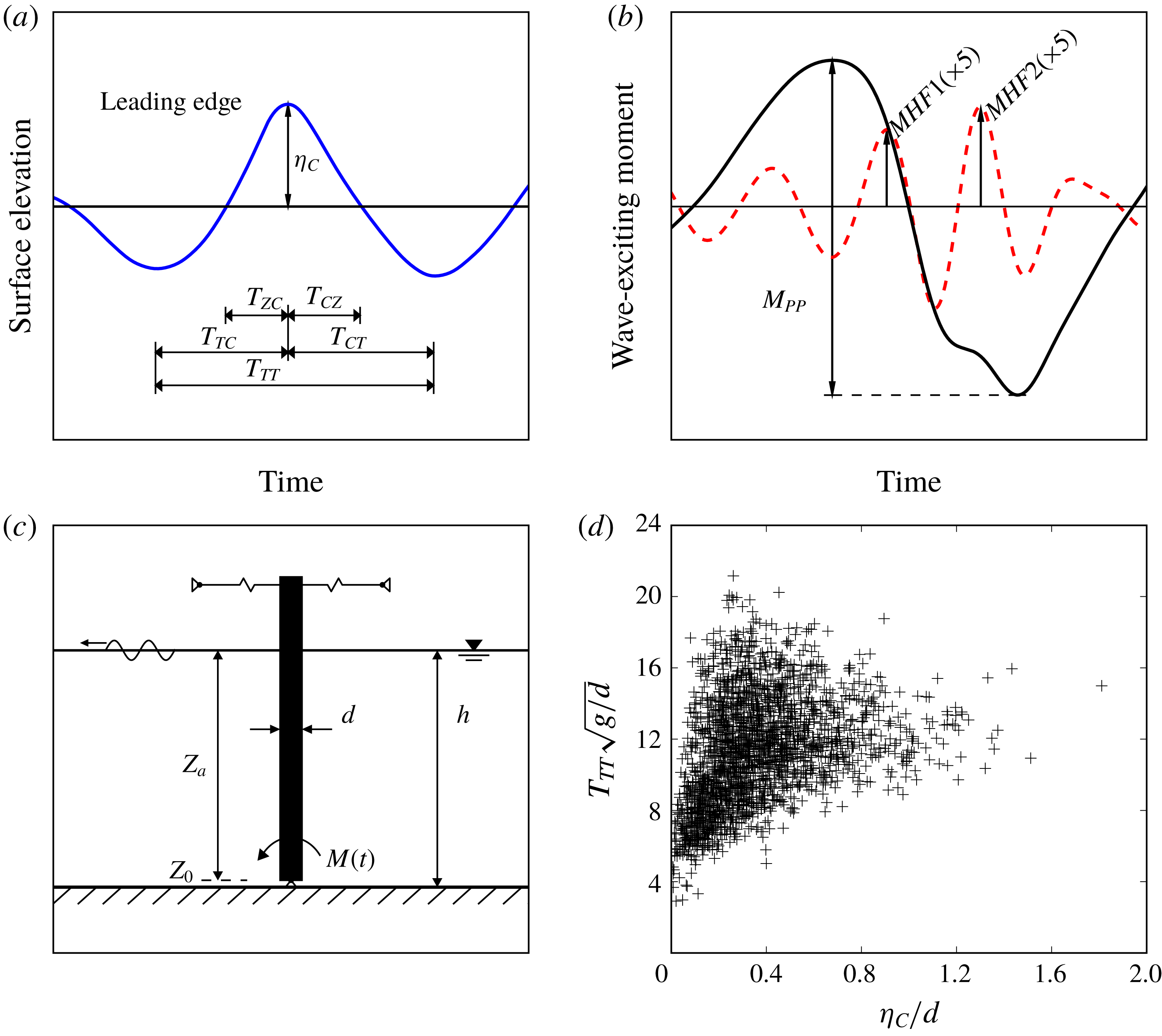
(a) The crest height
 $\unicode[STIX]{x1D702}_{C}$
, trough-to-trough period
 $T_{TT}$
, time from trough to crest
 $T_{TC}$
, zero upcrossing to crest
 $T_{ZC}$
, crest to trough
 $T_{CT}$
and crest to zero downcrossing
 $T_{CZ}$
; (b) the peak-to-peak load
 $M_{PP}$
, found from the total measured wave-exciting moment (——), and the high-frequency peaks
 $MHF1$
and
 $MHF2$
, found from the high-frequency part (– –) amplified by a factor of 5 (
 $\times 5$
); (c) cylinder set-up with diameter
 $d$
, water depth
 $h$
, rotation point
 $z_{0}$
, distance from rotation point to still water level
 $z_{a}$
and wave-exciting moment
 $M(t)$
; (d) wave scatter plot with
 $\unicode[STIX]{x1D702}_{C}$
and
 $T_{TT}$
(
 $+$
).

2 Methodology
A total of 2166 single wave events have been found from a set of laboratory experiments with a cylinder exposed to irregular deep water waves. The experiments, described in § 2.1, obtain the wave-exciting moment experienced by the cylinder about the rotation point
 $z_{0}$
; see figure 1(c). The high-frequency forces above a harmonic frequency of
 $3.5\unicode[STIX]{x1D714}_{TT}$
, where
 $\unicode[STIX]{x1D714}_{TT}=2\unicode[STIX]{x03C0}/T_{TT}$
and
 $T_{TT}$
is the trough-to-trough period of the local wave, see figure 1(a), are considered for each of the single events. A time window of
 ${\sim}20$
wave periods is used, where a general cutoff is applied at
 $\unicode[STIX]{x1D714}=60~\text{rad}~\text{s}^{-1}$
, which includes the sixth harmonic force for the majority of the waves, i.e. for
 $T_{TT}\sqrt{g/d}>8$
. The identified high-frequency forces clearly include the effects of slamming due to the steep and breaking waves, and also the secondary load cycle.
For a single wave event,
 $MHF1$
and
 $MHF2$
are the two most pronounced peaks found from the high-frequency part of the wave-exciting moment; see figure 1(b). In figure 1(b), the high-frequency part has been amplified by a factor of five for better visualization. The first peak, denoted by
 $MHF1$
, is found when the total load is positive and associated with the wave crest. The second peak, denoted by
 $MHF2$
, is found when the total load is negative and defines the secondary load cycle. In figure 1(b), we also define the peak-to-peak moment,
 $M_{PP}$
.
2.1 Experiments
The experiments (Riise et al.
Reference Riise, Grue, Jensen and Johannessen2018) where carried out in the hydrodynamic laboratory at the University of Oslo in a 25 m long and 0.5 m wide wave flume. The water depth was
 $h=0.72$
m. In one end of the tank, there was a piston type of wavemaker which was generating irregular waves. In the opposite end, there was a passively absorbing beach.
At a distance of 10.90 m from the wavemaker, a vertical surface-piercing cylinder with a diameter of
 $d=6$
cm was hinged at a horizontal lateral axis
 $2$
cm above the tank bottom; see figure 1(c). The top of the cylinder was connected to load cells (Hottinger Baldwin Messtechnik Type Z6C2 with 10 kg
 $\hat{=}\,2~\text{mV}~\text{V}^{-1}$
and 400 Hz sampling rate), measuring the force from which the wave-exciting moment
 $M(t)$
was determined. The accuracy of the load cells is
 ${<}0.01$
Nm, which is
 ${<}3\,\%$
with regards to the standard deviation of the measured load time series. The undisturbed waves were measured at the cylinder location with the cylinder removed, using ultrasound wave probes (UltraLab ULS Advanced Ultrasound, USS02/HFP with 250 Hz sampling rate). The accuracy of the wave probes is
 ${<}1$
mm, which is
 ${<}2$
% with regards to the cylinder diameter.
The experimental data consist of six irregular long-crested wave time series, each 320 s long, based on the JONSWAP spectrum (Hasselmann et al.
Reference Hasselmann, Barnett, Bouws, Carlson, Cartwright, Enke, Ewing, Gienapp, Hasselmann, Kruseman, Meerburg, Müller, Olbers, Richter, Sell and Walden1973) with peak enhancement factor
 $\unicode[STIX]{x1D6FE}=3.3$
. Each time series was repeated three times, and the median values are used to estimate the various parameters. The standard deviation of the measured crest heights over the three time series is typically 1.5 % of the cylinder diameter.
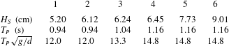
The wave spectral parameters are given in table 1, showing the significant wave height
 $H_{S}$
, the peak wave period
 $T_{P}$
and the normalized peak period
 $T_{P}\sqrt{g/d}$
, where
 $g$
is the acceleration due to gravity. These values are used to estimate the spectral steepness
 $0.5H_{S}k_{P}$
, normalized water depth
 $k_{P}h$
and wavelength
 $k_{P}r$
, where
 $r$
is the cylinder radius,
 $k_{P}$
is the peak wavenumber found using the linear dispersion relation
 $\unicode[STIX]{x1D714}_{P}^{2}=gk_{P}\tanh k_{P}h$
and
 $\unicode[STIX]{x1D714}_{P}=2\unicode[STIX]{x03C0}/T_{P}$
. This gives moderate to steep waves (
 $0.10<0.5H_{S}k_{P}<0.14$
) in deep water (
 $2.2<k_{P}h<3.3$
) outside the linear diffraction regime (
 $0.09<k_{P}r<0.14$
).
Spectral wave parameters for the six wave time series. Significant wave height
 $H_{S}$
, peak wave period
 $T_{P}$
and normalized period
 $T_{P}\sqrt{g/d}$
.

For the governing wave frequencies, the reflection coefficient, in terms of the amplitude as outlined by Goda & Suzuki (Reference Goda and Suzuki1976), is found to be less than 0.06. A small reflection from the beach primarily affects the force at the fundamental and second harmonic frequencies, and to a lesser extent higher harmonic forces (
 ${>}3\unicode[STIX]{x1D714}$
, where
 $\unicode[STIX]{x1D714}$
is the fundamental wave frequency) originating from wave effects at the waterline of the cylinder.
2.2 Wave parameter definitions
A single wave event is defined by the trough-to-trough period
 $T_{TT}$
and the crest height
 $\unicode[STIX]{x1D702}_{C}$
, as shown in figure 1(a). The 2166 single wave events are shown in the scatter plot in figure 1(d). For later purposes (§ 3.2), we define the Keulegan–Carpenter number
 $KC=2\unicode[STIX]{x03C0}\unicode[STIX]{x1D702}_{C}/d$
, governing flow separation effects, and the Froude number
 $Fr=U/\sqrt{gd}$
, governing free-surface gravity wave effects at the cylinder diameter scale. The flow velocity amplitude may be approximated by
 $U=2\unicode[STIX]{x03C0}\unicode[STIX]{x1D702}_{C}/T$
, where
 $T$
is the wave period. Furthermore, we define the leading wave edge, from trough to crest with the timing
 $T_{TC}$
, or from zero upcrossing to crest with
 $T_{ZC}$
. We also define the travelling wave edge, from crest to trough with
 $T_{CT}$
, or from crest to zero downcrossing with
 $T_{CZ}$
. In § 3.2, we relate the speed of the leading and travelling wave edges of the undisturbed wave to the flow velocity and Froude number. For this, an approximation of
 $U$
is suggested by
 $U=2\unicode[STIX]{x03C0}\unicode[STIX]{x1D702}_{C}/T_{i}$
, which gives
 $Fr=2\unicode[STIX]{x03C0}\unicode[STIX]{x1D702}_{C}/T_{i}\sqrt{gd}$
, where
 $T_{i}$
is given by
 $2T_{TC}$
,
 $4T_{ZC}$
,
 $2T_{CT}$
or
 $4T_{CZ}$
.
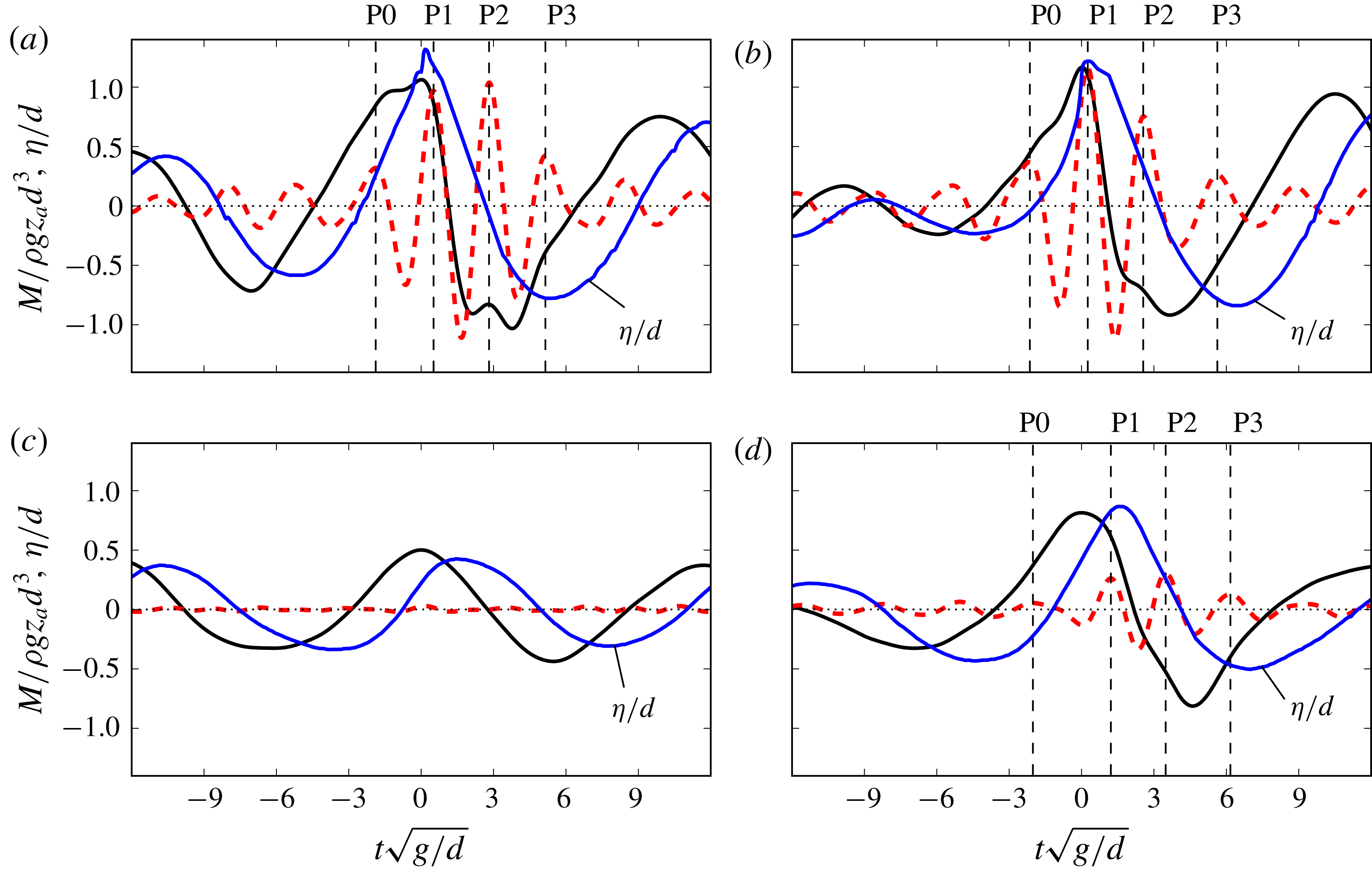
Surface elevation (——, blue), total measured wave-exciting moment (——) and high-frequency forces amplified by a factor of five (– –) for (a) series 1, with
 $(H_{S},T_{P})=$
(5.20 cm, 0.94 s), at
 $t=250.1$
s, (b) series 3, with
 $(H_{S},T_{P})=$
(6.24 cm, 1.04 s), at
 $t=155.7$
s, (c) series 1, with
 $(H_{S},T_{P})=$
(5.20 cm, 0.94 s), at
 $t=238.7$
s, and (d) series 3, with
 $(H_{S},T_{P})=$
(6.24 cm, 1.04 s), at
 $t=219.8$
s.

3 Results
We first illustrate the surface elevation and the wave-exciting moment for four typical wave events; see figure 2. The surface elevation
 $\unicode[STIX]{x1D702}$
is normalized by the cylinder diameter
 $d$
. The wave-exciting moment
 $M$
is normalized by
 $\unicode[STIX]{x1D70C}gz_{a}d^{3}$
, where
 $\unicode[STIX]{x1D70C}$
is the density of water,
 $g$
is the acceleration due to gravity and
 $z_{a}$
is the distance from the point of rotation to the still water level. The time
 $t$
is normalized by
 $\sqrt{g/d}$
. In the following,
 $^{\ast }$
denotes dimensionless values, i.e.
 $\unicode[STIX]{x1D702}^{\ast }=\unicode[STIX]{x1D702}/d$
,
 $M^{\ast }=M/\unicode[STIX]{x1D70C}gz_{a}d^{3}$
and
 $t^{\ast }=t\sqrt{g/d}$
.
In the first event (figure 2
a), with a crest height of
 $\unicode[STIX]{x1D702}_{C}^{\ast }=1.3$
and a wave period of
 $T_{TT}^{\ast }=10.4$
, we observe evidence of slamming due to the steep wave event. The maximum load has a value of
 $M^{\ast }=1.1$
and occurs approximately simultaneously with the wave crest. The minimum load has a value of
 $M^{\ast }=-1.0$
and occurs between the wave zero downcrossing and the following trough. This gives a peak-to-peak load of
 $M_{PP}^{\ast }=2.1$
and a time of
 $t^{\ast }=3.8$
between the maximum and minimum load peaks.
The high-frequency part of the wave-exciting moment, occurring during the local period of the load history (for
 $-4.5<t^{\ast }<6.4$
), consists of four peaks. The first peak (P0) is small. This occurs at
 $t^{\ast }=-2.0$
and is close in time to the wave zero upcrossing, where large inertia forces occur. The second peak (P1) is large, with
 $MHF1^{\ast }=0.19$
, and occurs at
 $t^{\ast }=0.4$
when the total load is positive. This is closely correlated in time with the wave crest, where large orbital velocity and wave breaking at the column occur. The third peak (P2) is also large, with
 $MHF2^{\ast }=0.20$
, occurring at
 $t^{\ast }=2.8$
when the total load is negative. This is associated with the secondary load cycle. The last peak (P3), which is small, occurring at
 $t^{\ast }=5.1$
, is close in time to the wave trough.
In the second event (figure 2
b), where
 $\unicode[STIX]{x1D702}_{C}^{\ast }=1.2$
and
 $T_{TT}^{\ast }=11.0$
, we observe evidence of slamming due to the breaking wave. The maximum load has a value of
 $M^{\ast }=1.2$
and the minimum load has a value of
 $M^{\ast }=-0.9$
. This gives
 $M_{PP}^{\ast }=2.1$
and
 $t^{\ast }=3.6$
between the extremes. The same distinct high-frequency peaks are observed with
 $MHF1^{\ast }=0.23$
at P1 and
 $MHF2^{\ast }=0.15$
at P2.
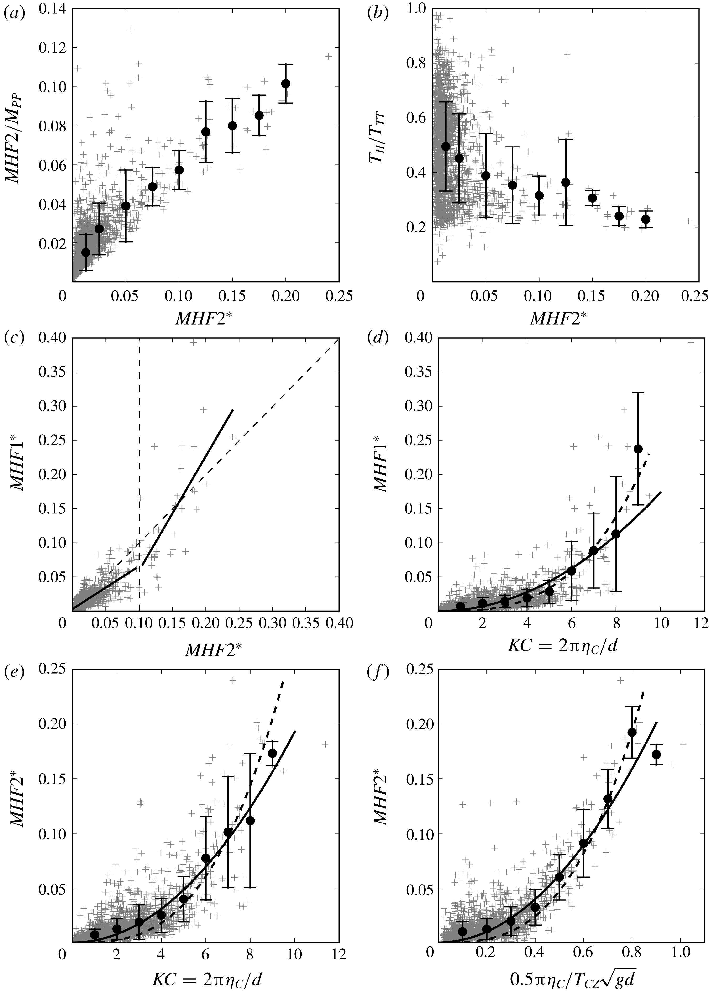
High-frequency force components and associated wave parameters in irregular waves. Single events (
 $+$
) and mean values (●), with bars corresponding to the standard deviation: (a) the magnitude of
 $MHF2^{\ast }$
relative to
 $M_{PP}^{\ast }$
; (b) the timing of
 $MHF2^{\ast }$
relative to
 $T_{TT}$
; (c) the magnitudes of
 $MHF2^{\ast }$
and
 $MHF1^{\ast }$
with fitted linear curves (——); (d)
 $MHF1^{\ast }$
as a function of
 $KC=2\unicode[STIX]{x03C0}\unicode[STIX]{x1D702}_{C}/d$
with fitted second- (——) and third- (– –) order curves; (e)
 $MHF2^{\ast }$
as a function of
 $KC$
; (f)
 $MHF2^{\ast }$
as a function of
 $Fr=0.5\unicode[STIX]{x03C0}\unicode[STIX]{x1D702}_{C}/T_{CZ}\sqrt{gd}$
.

Considering
 $MHF1^{\ast }$
and
 $MHF2^{\ast }$
for the two events (figures 2
a and 2
b), the time in between the peaks is
 $t^{\ast }=2.3$
and the magnitude is 7 %–11 % relative to
 $M_{PP}^{\ast }$
. In the first event,
 $MHF2^{\ast }$
is slightly larger than
 $MHF1^{\ast }$
, while in the second event,
 $MHF1^{\ast }$
is the largest. From the two events, it is found that the first of the two dominant peaks,
 $MHF1^{\ast }$
, occurs for
 $0<t^{\ast }<1$
(relative to the time of the maximum load), simultaneous to or shortly after the passing of the wave crest, when the total load is positive. Large orbital velocities and wave slamming due to the steep and breaking waves occur at the cylinder in this time range. The secondary load cycle,
 $MHF2^{\ast }$
, occurs for
 $2<t^{\ast }<3$
. This is approximately at the same time as the wave zero downcrossing. The total load is then negative.
A third event with no visible high-frequency force, where
 $MHF1^{\ast }\cong MHF2^{\ast }\cong 0.01$
, is shown in figure 2(c). For the fourth event, see figure 2(d), we observe small values of
 $MHF1^{\ast }\cong MHF2^{\ast }\cong 0.06$
. Regarding the secondary load cycle, it is generally observed that this becomes visible in the range
 $0.06<MHF2^{\ast }<0.10$
and is significant for
 $MHF2^{\ast }>0.10$
.
In a resonant build up of the motion response, a set of succeeding load cycles will amplify the response. As an illustration of the importance of the secondary load cycle, we may consider the time varying response
 $\unicode[STIX]{x1D709}(t)$
of an undamped oscillator exposed to a harmonic force
 $\cos (\unicode[STIX]{x1D714}_{0}t)$
, with
 $\unicode[STIX]{x1D714}_{0}$
the resonance frequency of the oscillator, expressed by the equation of motion
 $\ddot{\unicode[STIX]{x1D709}}(t)+\unicode[STIX]{x1D714}_{0}^{2}\unicode[STIX]{x1D709}(t)=\unicode[STIX]{x1D6FC}_{0}\cos (\unicode[STIX]{x1D714}_{0}t)$
. With a start from rest, the response increases according to
 $\unicode[STIX]{x1D709}(t)\propto t\sin (\unicode[STIX]{x1D714}_{0}t)$
. This shows that through one load cycle, the response is amplified by a factor equal to
 $t=2\unicode[STIX]{x03C0}/\unicode[STIX]{x1D714}_{0}$
, and that both the first and the second of the two large high-frequency peaks,
 $MHF1^{\ast }$
and
 $MHF2^{\ast }$
, are important.
3.1 Magnitude and period of the secondary load cycle
In the following, we consider the high-frequency force contributions for all of the 2166 events. Figures 3(a) and 3(b) present the magnitude and timing of the secondary load cycle
 $MHF2^{\ast }$
relative to the total load
 $M_{PP}^{\ast }$
. The magnitude ratio
 $MHF2/M_{PP}$
, as shown in figure 3(a), increases with regards to
 $MHF2^{\ast }$
, clearly indicating the nonlinear behaviour for the high-frequency force.
Furthermore, we observe that the magnitude for the large events (
 $MHF2^{\ast }>0.1$
) is up to 12 % of the peak-to-peak load. This shows that the present results, with the higher harmonic forces extracted from the wave-exciting moment, are comparable to previous published work, where the force ratio is reported. Grue et al. (Reference Grue, Bjørshol and Strand1993, Reference Grue, Bjørshol, Strand and Ohkusu1994) reported a magnitude up to 11 %, Chaplin et al. (Reference Chaplin, Rainey and Yemm1997) 8 %–12 % and Grue & Huseby (Reference Grue and Huseby2002) 10 %–15 %.
The timing of
 $MHF2^{\ast }$
with regards to the positive peak of the total load, shown in figure 3(b), seems to converge to around one quarter of a wave period. This is in good agreement with the results reported by Grue & Huseby (Reference Grue and Huseby2002), and generalizes the previous findings obtained in regular waves to the case of irregular waves.
The difference in magnitude between the high-frequency force peak close in time to the wave crest,
 $MHF1^{\ast }$
(P1), and the secondary load cycle,
 $MHF2^{\ast }$
(P2), is shown in figure 3(c). We observe that for events with small forces (
 $MHF2^{\ast }<0.15$
and
 $MHF1^{\ast }<0.15$
), it is mostly the force associated with the secondary load cycle that is the largest, i.e
 $MHF2^{\ast }>MHF1^{\ast }$
.
When the forces that occur at the same time as the wave crest become large (
 $MHF1^{\ast }>0.15$
), they also become more dominant, and for the largest forces we observe that the peak P1 is larger than the peak P2 (
 $MHF1^{\ast }>MHF2^{\ast }$
). Observations show that these events include evidence of slamming due to steep and breaking waves. The difference between the magnitudes of P1 and P2 is further visualized by two linear curves fitted to the data. The first curve is fitted to events where
 $MHF2^{\ast }<0.1$
and the second curve is fitted to events where
 $MHF2^{\ast }>0.1$
.
3.2 Keulegan–Carpenter number versus gravity effects
The effect of flow separation is considered by investigating the forces as a function of the Keulegan–Carpenter number
 $KC$
. Figure 3(d) shows the behaviour of the high-frequency force peak (P1) close in time to the wave crest,
 $MHF1^{\ast }$
. The ensemble mean and standard deviation are found together with the second- and third-order curves
 $\unicode[STIX]{x1D6FC}_{2}x^{2}$
and
 $\unicode[STIX]{x1D6FC}_{3}x^{3}$
respectively for
 $x=KC$
, estimated by least squares. For
 $KC<5$
, the force mean shows an approximately linear behaviour. Around
 $KC\sim 5$
, it appears to change to a more rapid growth, and for
 $KC>5$
the mean shifts between the higher-order curves. A large scatter is observed. For comparison, we define the coefficient of variation,
 $CV$
, by
 $$\begin{eqnarray}CV=\sqrt{\frac{1}{N}\mathop{\sum }_{i=1}^{N}\left(\frac{y_{i,meas}-y_{i,curve}}{y_{i,curve}}\right)^{2}},\end{eqnarray}$$
where
 $y_{i,meas}$
is the measurement,
 $y_{i,curve}$
is the fitted curve and
 $N$
is the number of events. We consider
 $KC>5$
,
 $CV=0.61$
and
 $0.60$
for the second- and third-order curves respectively.
The behaviour of the secondary load cycle,
 $MHF2^{\ast }$
(P2), as a function of
 $KC$
, is shown in figure 3(e). Similarly to the behaviour of
 $MHF1^{\ast }$
, the force mean shows an approximately linear behaviour for
 $KC<4$
, a change to a more rapid growth for
 $KC\sim 4$
–5, and for
 $KC>5$
we observe that the force mean shifts between the two higher-order curves. The coefficient of variation is
 $CV=0.48$
and
 $0.55$
for the fitted second- and third-order curves respectively for
 $KC>5$
.
In figure 3(f), free-surface gravity wave effects on the cylinder scale are considered by investigating
 $MHF2^{\ast }$
as a function of the Froude number
 $Fr$
. The secondary load cycle appears close in time to the wave zero downcrossing, which suggests the use of the speed of the travelling edge of the undisturbed wave to define the wave parameters. Then, an improved estimate of the Froude number is suggested by
 $Fr=0.5\unicode[STIX]{x03C0}\unicode[STIX]{x1D702}_{C}/T_{CZ}\sqrt{gd}$
. Here,
 $T_{CZ}$
is the time between the crest and the zero downcrossing. The measurements are compared with second- and third-order fitted curves,
 $\unicode[STIX]{x1D6FC}_{2}x^{2}$
and
 $\unicode[STIX]{x1D6FC}_{3}x^{3}$
respectively, for
 $x=Fr$
. We observe the same trends as outlined above for
 $KC$
. There is a close to linear behaviour when
 $Fr<0.3$
, a more rapid growth occurs around
 $Fr\sim 0.3$
–0.4, and the force mean shifts from the second- to the third-order curve for
 $Fr>0.4$
. The proxy with
 $Fr$
shows considerably less scatter for the large forces, compared with the results for
 $KC$
.
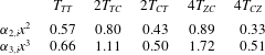
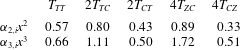
All of the periods defined in § 2.1 and figure 1(c) were analysed with the resulting
 $CV$
listed in table 2. The best correlation,
 $CV=0.33$
, was found using the time between the crest and the zero downcrossing,
 $T_{CZ}$
, as shown in figure 3(f). Although it is not evident which among the two discussed effects governs the secondary load cycle, it is clear that the flow velocity is an important parameter. Furthermore, the good correlation with the speed of the travelling edge of the undisturbed wave indicates that the asymmetry of the wave may be important.
Regarding the peak
 $MHF1^{\ast }$
(P1), the same tendencies are observed when the function is analysed as a function of
 $Fr$
. The best correlation was again found using the travelling edge of the undisturbed wave to define
 $Fr$
.
The coefficient of variation,
 $CV$
, for fitted second- (
 $\unicode[STIX]{x1D6FC}_{2,i}x^{2}$
) and third- (
 $\unicode[STIX]{x1D6FC}_{3,i}x^{3}$
) order curves for
 $x=MHF2$
and
 $Fr=2\unicode[STIX]{x03C0}\unicode[STIX]{x1D702}_{C}/T_{i}\sqrt{gd}>0.4$
with different wave period definitions
 $T_{i}$
.
4 Conclusions
A set of laboratory experiments with a bottom hinged cylinder, exposed to irregular deep water waves, was used to study the strongly nonlinear high-frequency forcing, with a focus on the secondary load cycle. We considered the forces above a harmonic frequency of
 $3.5\unicode[STIX]{x1D714}_{TT}$
, where
 $\unicode[STIX]{x1D714}_{TT}=2\unicode[STIX]{x03C0}/T_{TT}$
, and
 $T_{TT}$
is the trough-to-trough period of the local wave. Two pronounced high-frequency force peaks have been identified. The first peak, P1, is closely correlated in time with the wave crest. At this time, large orbital velocity is present and slamming due to steep and breaking waves may occur. The second peak, P2, defines the secondary load cycle. The high-frequency force peaks were studied for 2166 events and related to local wave parameters. This enabled a systematic study of the forces with respect to the two dimensionless parameters, the Keulegan–Carpenter number (
 $KC$
), governing for flow separation, and the Froude number (
 $Fr$
), governing for free-surface gravity wave effects. The two high-frequency peaks were investigated by means of regression analysis.
Regarding the secondary load cycle, both
 $KC$
, indicating flow separation effects, and
 $Fr$
, indicating the effect of surface gravity waves, were found to be important. Best correlation was found between the secondary load cycle and
 $Fr$
. The speed of the travelling edge of the undisturbed wave was used to approximate the fluid velocity. A threshold value separating small and large force peaks was found for
 $KC\sim 4$
–5 or, alternatively, for
 $Fr\sim 0.3$
–0.4, indicating a change in the physical mechanisms that govern the high-frequency force. Although it is not clear which of the two effects dominates, it is clear that the flow velocity is an important parameter for the secondary load cycle. The magnitude of the secondary load cycle was found to be up to
 ${\sim}12\,\%$
of the peak-to-peak load. The secondary load cycle was found to occur around one quarter of the wave period after the peak of the total load. This generalizes, to the case of irregular waves, previous findings obtained in regular waves.
Acknowledgements
This study was carried out with financial support from Stiftelsen Det Norske Veritas, DNV GL and The Research Council of Norway. The technical assistance during the experimental work by Head Engineer O. Gundersen is gratefully acknowledged.