1. Introduction
An understanding of the dynamics of the impact of a layer of fluid with a solid boundary is important in a number of practical applications, including any form of sea defence (e.g. the impact of a tide on a tidal barrage), dam breaking during earthquakes, sloshing in tanks and containers, and in ship design. Of particular interest in such scenarios is the structure of flow in the locality of the free surface and solid boundary where typically jet formation is observed. In particular, fluid–structure interactions for partially filled containers have numerous applications to the aerospace industry (Veldman et al. Reference Veldman, Gerrits, Luppes, Helder and Vreeburg2007) and to naval and air transport (Liu & Lin Reference Liu and Lin2009). In some cases, usually where the interaction is violent in nature, as in splashing and ship slamming (Korobkin & Pukhnachov Reference Korobkin and Pukhnachov1988; Purvis & Smith Reference Purvis and Smith2005), the structure of the jet will evolve over highly refined spatial and temporal scales. This may be seen, for example, in the case where a droplet impacts with finite speed on a solid substrate, leading to the formation of an ejecta sheet caused by a localized pressure singularity (see Howison et al. Reference Howison, Ockendon, Oliver, Purvis and Smith2005). A similar scenario occurs when a solid body impacts onto a layer of fluid, as investigated by Iafrati & Korobkin (Reference Iafrati and Korobkin2004), who considered the asymptotic structure of the flow generated by the impact of a flat plate on a liquid free surface. Whilst numerical methods provide a gateway to understanding some of the inherent features present in such problems (see Greenhow Reference Greenhow1993), the need for very fine spatial resolutions to accurately model the evolution of a jet caused by an impulsively or violently moved body into a layer of fluid can be very prohibitive. Additionally, with various numerical methods available for the treatment of such fluid–structure interactions, the validation of results with theoretical analysis very close to the contact point provides a good way of demonstrating the validity and applicability of a given computational model (Rebouillat & Liksonov Reference Rebouillat and Liksonov2010). In all such cases, an analytical approach may be useful and can be used to determine the order of magnitudes for jet thickness and strength (momentum flux).
The transient motion near the point of contact between a surface-piercing solid body and a free surface was considered by Roberts (Reference Roberts1987), who examined the development of a dispersive wavetrain for power-law displacements of a vertical plate adjacent to the free surface. Subsequently Chwang (Reference Chwang1983) determined the nonlinear hydrodynamic pressure on an accelerating vertical plate, obtaining an analytical solution using small-time expansions. An extension of the analysis of Roberts (Reference Roberts1987) to include the effects of capillarity on the train of short-wavelength dispersive waves observed near the moving boundary was presented by Joo, Schultz & Messiter (Reference Joo, Schultz and Messiter1990). Norkin & Korobkin (Reference Norkin and Korobkin2011) have examined the initial flow caused by an impulsively moved partially submerged circular cylinder. The full early-stage structure and dynamics of a free surface interacting with an accelerated vertical rigid plate has been investigated by King & Needham (Reference King and Needham1994) and Needham, Chamberlain & Billingham (Reference Needham, Chamberlain and Billingham2008). In both of these cases the fluid was considered to be inviscid and incompressible and without surface tension. King & Needham (Reference King and Needham1994) considered the case of a uniformly accelerated plate and investigated the resultant thin jet that moves up the plate. They derived an analytical solution for the flow field for small times
 $t$
. This work was extended by Needham, Billingham & King (Reference Needham, Billingham and King2007) to include the case where the plate is moved impulsively. Recently Needham et al. (Reference Needham, Chamberlain and Billingham2008) have considered the corresponding situation where the inclination of the plate to the exterior horizontal,
 ${\it\alpha}$
, was generalized so as to include the cases where
 ${\it\alpha}\in (0,{\rm\pi}/2)\cup ({\rm\pi}/2,{\rm\pi})$
. It was found that for the case where the angle is acute,
 ${\it\alpha}\in (0,{\rm\pi}/2)$
, a jet of thickness of
 $O(t^{2})$
as
 $t\rightarrow 0^{+}$
rises up the plate, with the free surface slope at the contact point being of
 $O(t^{{\rm\pi}/{\it\alpha}-2})$
as
 $t\rightarrow 0^{+}$
. This is in contrast to the case when the plate is vertical, where the jet has a thickness of
 $O(t^{2}\ln t)$
and free surface slope of
 $O(1/\!\ln t)$
as
 $t\rightarrow 0^{+}$
. For the case where the angle is obtuse,
 ${\it\alpha}\in ({\rm\pi}/2,{\rm\pi})$
, it was found that the thickness of the jet was given by
 $O(t^{{\it\gamma}})$
, where
 ${\it\gamma}=(1-{\rm\pi}/4{\it\alpha})^{-1}$
with slope
 $O(1)$
as
 $t\rightarrow 0^{+}$
. In summary, therefore, the jet becomes stronger and takes a much more nonlinear structure, with thickness depending on
 ${\it\alpha}$
, as
 ${\it\alpha}$
is increased through
 ${\rm\pi}/2$
. Moreover, classical solutions were only obtainable when
 ${\it\alpha}\in ({\rm\pi}/2,{\it\alpha}_{c}]$
, where
 ${\it\alpha}_{c}\approx 1.791\approx 102.6^{\circ }$
. For the special case where
 ${\it\alpha}={\it\alpha}_{c}$
, a corner forms at the contact point at
 $t=0^{+}$
and convects self-similarly into the inner region for
 $0<t\ll 1$
. This prevents continuation of the classical solution for angles
 ${\it\alpha}\in ({\it\alpha}_{c},{\rm\pi})$
. The effects of surface tension may allow for the possibility of classical solutions existing in the neighbourhood of
 $t=0^{+}$
when
 ${\it\alpha}\in ({\it\alpha}_{c},{\rm\pi})$
.
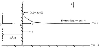
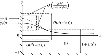
A sketch showing the displacement of the plate and the free surface at time
 $t>0$
. The translating coordinate system
 $(\bar{x},y)$
is also shown.

As a consequence, and a prelude to considering plate angles
 ${\it\alpha}\in (0,{\rm\pi}/2)\cup ({\rm\pi}/2,{\rm\pi})$
, in this paper we consider the dynamics of the free surface and plate intersection point (which we henceforth refer to as the contact point) for small time
 $t$
and weak surface tension, via the method of matched asymptotic expansions for the case where
 ${\it\alpha}={\rm\pi}/2$
. The paper is organized as follows. In § 2 we formulate the governing equations and boundary conditions and establish the initial–boundary value problem (IBVP) that is to be investigated. The solution of this problem as
 $t\rightarrow 0^{+}$
is examined in § 3, which can be considered as an extension of the work of King & Needham (Reference King and Needham1994), and is necessary here to motivate and provide information for the work that follows later. In § 4 we consider the local structure of the flow near the contact point. In § 5 we introduce surface tension, characterized by the inverse Weber number
 $\mathscr{W}$
, and consider the revised initial–boundary value problem
 $(\text{IBVP})^{\prime }$
, for which we examine the weak surface tension limit. This leads to a linear time-dependent harmonic problem, which we numerically solve in § 6. In § 7 we present the asymptotic structure of the solutions to
 $(\text{IBVP})^{\prime }$
as
 $\mathscr{W}\rightarrow 0$
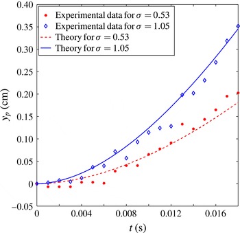
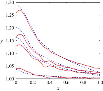
, along with key characteristics of the jet close to the plate. Finally, in § 9 we present some preliminary experimental results, which show both the rise of the jet at the contact point as well as the free surface profiles near the contact point, and we make favourable comparisons with the theoretical results obtained in §§ 7 and 8.
2. Problem formulation
We first consider the motion of an initially stationary layer of inviscid fluid when the layer is disturbed by a bounding vertical plate accelerating from rest into the region initially occupied by the layer, as shown in figure 1. The foregoing analysis is an extension of King & Needham (Reference King and Needham1994) and is needed here to motivate and provide additional results for the analysis in § 5. In particular, in this section, we consider the case where the surface tension
 $T=0$
. We consider this problem in the fixed Cartesian coordinates shown in figure 1, where
 $x$
points horizontally into the fluid layer and
 $y$
points vertically upwards, and throughout we measure fluid velocities relative to this rest frame. In this coordinate system, the free surface can be described by
 $y={\it\eta}(x,t)$
and the rigid bed by
 $y=-h$
, where
 $t$
is time and
 $h>0$
. Initially the fluid domain is bounded by a vertical rigid plate at
 $x=0$
and the fluid lies stationary in the region
 $(x,y)\in [0,\infty )\times [-h,0]$
. At
 $t=0$
the plate is translated in the positive
 $x$
direction with constant acceleration
 $a>0$
. The contact point and the bed are denoted by
 $(x_{p}(t),{\it\eta}(x_{p}(t),t))$
and
 $(x_{p}(t),-h)$
, respectively, with
 $x_{p}(t)=at^{2}/2$
for
 $t\geqslant 0$
.
The fluid motion when
 $t>0$
will be irrotational, since the fluid is at rest when
 $t=0$
, and hence there exists a velocity potential
 ${\it\phi}(x,y,t)$
. We denote the fluid pressure by
 $p(x,y,t)$
. It is convenient to introduce dimensionless variables
 $$\begin{eqnarray}x^{\prime }=\frac{x}{h},\quad y^{\prime }=\frac{y}{h},\quad {\it\eta}^{\prime }=\frac{{\it\eta}}{h},\quad {\it\phi}^{\prime }=\frac{{\it\phi}}{h\sqrt{gh}},\quad p^{\prime }=\frac{p}{{\it\rho}gh},\quad t^{\prime }=t\sqrt{\frac{g}{h}},\end{eqnarray}$$
where
 $g$
is the acceleration due to gravity and
 ${\it\rho}$
is the constant fluid density. For convenience in notation, we henceforth drop the primes. It is also convenient to introduce the coordinate
 $\bar{x}$
defined by
 $\bar{x}=x-s(t)$
in
 $t\geqslant 0$
, where
 $s(t)={\it\sigma}t^{2}/2$
with the dimensionless parameter
 ${\it\sigma}=a/g$
, which measures the dimensionless acceleration of the plate and is strictly positive, whilst
 $s(t)$
is the horizontal displacement of the vertical plate from its initial position. In the
 $(\bar{x},y)$
coordinate system the location of the plate is at
 $\bar{x}=0$
for all
 $t\geqslant 0$
(note that in the
 $(\bar{x},y)$
coordinate system, with origin in the plate, we will still measure fluid velocity fields relative to the stationary frame of reference). The region occupied by the fluid, for
 $t\geqslant 0$
, can be expressed as
 $$\begin{eqnarray}\mathscr{D}(t)=\{(\bar{x},y)\in \mathbb{R}^{2}:\bar{x}>0,-1<y<{\it\eta}(\bar{x},t)\}.\end{eqnarray}$$
It should also be noted that in this translating coordinate system we have
 $$\begin{eqnarray}\bar{x}_{p}(t)=0\quad \text{and}\quad y_{p}(t)={\it\eta}(\bar{x}_{p}(t),t)={\it\eta}(0,t),\end{eqnarray}$$
for
 $t\geqslant 0$
. The governing field equation for this problem is given by
 $$\begin{eqnarray}{\rm\nabla}^{2}{\it\phi}=0,\quad (\bar{x},y)\in \mathscr{D}(t),t>0.\end{eqnarray}$$
At the plate we have
 $$\begin{eqnarray}{\it\phi}_{\bar{x}}={\dot{s}}(t),\quad \bar{x}=0,-1<y<{\it\eta}(0,t),t>0.\end{eqnarray}$$
The bed is impermeable so that
 $$\begin{eqnarray}{\it\phi}_{y}=0,\quad y=-1,\bar{x}>0,t>0.\end{eqnarray}$$
The kinematic condition at the free surface can be written as
 $$\begin{eqnarray}{\it\eta}_{t}+[{\it\phi}_{\bar{x}}-{\dot{s}}(t)]{\it\eta}_{\bar{x}}-{\it\phi}_{y}=0,\quad y={\it\eta}(\bar{x},t),\bar{x}>0,t>0,\end{eqnarray}$$
whilst Bernoulli’s equation at the free surface, where the pressure is taken to be zero, gives the condition,
 $$\begin{eqnarray}{\it\phi}_{t}-{\dot{s}}(t){\it\phi}_{\bar{x}}+{\textstyle \frac{1}{2}}|\boldsymbol{{\rm\nabla}}{\it\phi}|^{2}+{\it\eta}=0,\quad y={\it\eta}(\bar{x},t),\bar{x}>0,t>0.\end{eqnarray}$$
Finally, at large distances from the plate we require
 $$\begin{eqnarray}\displaystyle & \displaystyle |\boldsymbol{{\rm\nabla}}{\it\phi}|\rightarrow 0\quad \text{as }\bar{x}\rightarrow \infty ,\text{uniformly for }-1\leqslant y\leqslant {\it\eta}(\bar{x},t),t>0, & \displaystyle\end{eqnarray}$$
 $$\begin{eqnarray}\displaystyle & \displaystyle {\it\eta}\rightarrow 0\quad \text{as }\bar{x}\rightarrow \infty ,t>0. & \displaystyle\end{eqnarray}$$
 $$\begin{eqnarray}\displaystyle & \displaystyle {\it\phi}(\bar{x},y,0)=0,\quad (\bar{x},y)\in \bar{\mathscr{D}}(0), & \displaystyle\end{eqnarray}$$
 $$\begin{eqnarray}\displaystyle & \displaystyle {\it\eta}(\bar{x},0)=0,\quad \bar{x}\geqslant 0. & \displaystyle\end{eqnarray}$$
 $$\begin{eqnarray}p=p_{d}-y,\quad (\bar{x},y)\in \bar{\mathscr{D}}(t),t>0,\end{eqnarray}$$
where
 $p_{d}$
is the dynamic fluid pressure field, which, via the Bernoulli equation, is given by
 $$\begin{eqnarray}p_{d}=-{\it\phi}_{t}+{\dot{s}}(t){\it\phi}_{\bar{x}}-{\textstyle \frac{1}{2}}|\boldsymbol{{\rm\nabla}}{\it\phi}|^{2},\quad (\bar{x},y)\in \bar{\mathscr{D}}(t),t>0.\end{eqnarray}$$
Our aim in the following two sections is to examine classical solutions to the initial–boundary value problem (2.4)–(2.14) (henceforth referred to as [IBVP]), in the sense that we impose the regularity conditions
 $$\begin{eqnarray}{\it\phi}\in C(\bar{\mathscr{G}})\cap C^{1}(\mathscr{G}\cup \partial \mathscr{G})\cap C^{2}(\mathscr{G}),\quad {\it\eta}\in C(\bar{\mathscr{H}})\cap C^{1}(\mathscr{H}),\end{eqnarray}$$
where
 $$\begin{eqnarray}\displaystyle & \mathscr{G}=\{(\bar{x},y,t)\in \mathbb{R}^{3}:(\bar{x},y)\in \mathscr{D}(t),t\in (0,\infty )\}, & \displaystyle\end{eqnarray}$$
 $$\begin{eqnarray}\displaystyle & \partial \mathscr{G}=\{(\bar{x},y,t)\in \mathbb{R}^{3}:(\bar{x},y)\in \bar{\mathscr{D}}(t)\setminus \mathscr{D}(t),t\in (0,\infty )\}, & \displaystyle\end{eqnarray}$$
 $$\begin{eqnarray}\displaystyle & \mathscr{H}=\{(\bar{x},t)\in \mathbb{R}^{2}:\bar{x}\in [0,\infty ),t\in (0,\infty )\}. & \displaystyle\end{eqnarray}$$
3. Asymptotic structure for [IBVP] as
 $t\rightarrow 0^{+}$

In this section we consider the asymptotic solution to [IBVP] as
 $t\rightarrow 0^{+}$
. We begin by considering an outer region in which
 $(\bar{x},y)\in \bar{\mathscr{D}}(t)=O(1)$
as
 $t\rightarrow 0^{+}$
, after which we require an inner region to complete the structure, in which
 $(\bar{x},y)\in \bar{\mathscr{D}}(t)=o(1)$
as
 $t\rightarrow 0^{+}$
.
3.1. Outer region as
$t\rightarrow 0^{+}$

By considering (2.5) and (2.7), together with the expression for
 $s(t)={\textstyle \frac{1}{2}}{\it\sigma}t^{2}$
, we require that
 ${\it\phi}=O(t)$
and
 ${\it\eta}=O(t^{2})$
as
 $t\rightarrow 0^{+}$
in the outer region. It is therefore appropriate that we introduce asymptotic expansions of the form
 $$\begin{eqnarray}{\it\phi}(\bar{x},y,t)=t{\it\sigma}\bar{{\it\phi}}(\bar{x},y)+O(t^{2}),\quad {\it\eta}(\bar{x},t)=t^{2}\bar{{\it\eta}}(\bar{x})+O(t^{3}),\end{eqnarray}$$
uniformly as
 $t\rightarrow 0^{+}$
in the outer region. The factor
 ${\it\sigma}$
in (3.1) is included for algebraic convenience at a later stage. Substitution of (3.1) into [IBVP] leads to the following leading-order problem for
 $\bar{{\it\phi}}$
, namely,
 $$\begin{eqnarray}\displaystyle & {\rm\nabla}^{2}\bar{{\it\phi}}=0,\quad (\bar{x},y)\in \mathscr{D}(0), & \displaystyle\end{eqnarray}$$
 $$\begin{eqnarray}\displaystyle & \bar{{\it\phi}}_{\bar{x}}=1,\quad \bar{x}=0,-1<y<0, & \displaystyle\end{eqnarray}$$
 $$\begin{eqnarray}\displaystyle & \bar{{\it\phi}}_{y}=0,\quad y=-1,\bar{x}>0, & \displaystyle\end{eqnarray}$$
 $$\begin{eqnarray}\displaystyle & \bar{{\it\phi}}=0,\quad y=0,\bar{x}>0, & \displaystyle\end{eqnarray}$$
 $$\begin{eqnarray}\displaystyle & |\boldsymbol{{\rm\nabla}}\bar{{\it\phi}}|\rightarrow 0\quad \text{as }\bar{x}\rightarrow \infty ,\text{uniformly for }-1\leqslant y\leqslant 0, & \displaystyle\end{eqnarray}$$
 $\bar{{\it\eta}}$
is given by
 $$\begin{eqnarray}\bar{{\it\eta}}(\bar{x})=\frac{{\it\sigma}}{2}\bar{{\it\phi}}_{y}(\bar{x},0),\quad \bar{x}\geqslant 0.\end{eqnarray}$$
Thus
 $\bar{{\it\phi}}$
is the solution to the harmonic boundary value problem (3.2), defined on the fixed semi-infinite rectangular domain
 $\bar{\mathscr{D}}(0)$
, and according to (2.15) we would require
 ${\it\phi}\in C(\bar{D}(0))\cap C^{1}(\bar{D}(0))\cap C^{2}(D(0))$
. However, a solution with this regularity cannot exist due to the boundary conditions (3.2b
) and (3.2d
). This reflects the non-uniformity in asymptotic expansions (3.1) when
 $(\bar{x},y)=o(1)$
as
 $t\rightarrow 0^{+}$
. To proceed, we relax regularity for this harmonic boundary value problem to
 $$\begin{eqnarray}\displaystyle & \displaystyle \bar{{\it\phi}}\in C(\bar{\mathscr{D}}(0))\cap C^{1}(\bar{\mathscr{D}}(0)\setminus \{0,0\})\cap C^{2}(\mathscr{D}(0))\quad \text{and} & \displaystyle \nonumber\\ \displaystyle & \displaystyle |\boldsymbol{{\rm\nabla}}\bar{{\it\phi}}|~\text{has at worst an integrable singularity at }(\bar{x},y)=(0,0). & \displaystyle\end{eqnarray}$$
Under this regularity, (3.2) has a unique solution, and this can be obtained explicitly via the method of separation of variables to give
 $$\begin{eqnarray}\bar{{\it\phi}}(\bar{x},y)=\frac{8}{{\rm\pi}^{2}}\mathop{\sum }_{n=0}^{\infty }\frac{1}{(2n+1)^{2}}\,\text{e}^{-(n+1/2){\rm\pi}\bar{x}}\sin \left[\left(n+\frac{1}{2}\right)\!{\rm\pi}y\right],\quad (\bar{x},y)=\bar{D}(0),\end{eqnarray}$$
after which we obtain from (3.3)
 $$\begin{eqnarray}\bar{{\it\eta}}(\bar{x})=\frac{2{\it\sigma}}{{\rm\pi}}\mathop{\sum }_{n=0}^{\infty }\frac{1}{(2n+1)}\,\text{e}^{-(n+1/2){\rm\pi}\bar{x}},\quad \bar{x}>0.\end{eqnarray}$$
This infinite series may be conveniently summed to arrive at
 $$\begin{eqnarray}\bar{{\it\eta}}(\bar{x})=\frac{{\it\sigma}}{{\rm\pi}}\ln \left(\coth \left(\frac{{\rm\pi}\bar{x}}{4}\right)\right),\quad \bar{x}>0.\end{eqnarray}$$
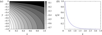
We plot contours of the potential
 $\bar{{\it\phi}}(\bar{x},y)$
and the free surface disturbance
 $\bar{{\it\eta}}(\bar{x})$
in figure 2. We observe that, as
 $\bar{x}\rightarrow 0$
, we have
 $\bar{{\it\eta}}(\bar{x})\rightarrow \infty$
. Accordingly, we now examine the local behaviour of
 $\bar{{\it\phi}}(\bar{x},y)$
near the origin
 $(\bar{x},y)=(0,0)$
by solving Laplace’s equation in polar coordinates in the quarter-plane
 $0<r<1$
and
 $-{\rm\pi}/2<{\it\theta}<0$
(with
 $\bar{x}=r\cos {\it\theta}$
and
 $\bar{y}=r\sin {\it\theta}$
) subject to the boundary conditions (3.2b
) and (3.2d
). It follows that the solution (3.5) must have the structure
 $$\begin{eqnarray}\bar{{\it\phi}}(r,{\it\theta})=-\frac{2}{{\rm\pi}}(r\ln r)\sin {\it\theta}-\frac{2}{{\rm\pi}}r{\it\theta}\cos {\it\theta}+\mathop{\sum }_{n=0}^{\infty }A_{n}r^{(2n+1)}\sin ((2n+1){\it\theta}),\end{eqnarray}$$
with
 $0\leqslant r<1$
and
 $-{\rm\pi}/2\leqslant {\it\theta}\leqslant 0$
, where
 $A_{n}\in \mathbb{R}$
are constants. This exhibits a weak singularity in
 $\boldsymbol{{\rm\nabla}}\bar{{\it\phi}}(r,{\it\theta})$
as
 $r\rightarrow 0$
. The local behaviour of
 $\bar{{\it\phi}}(\bar{x},y)$
near
 $(\bar{x},y)=(0,-1)$
can be investigated in a similar manner to establish that the solution (3.5) must have the structure
 $$\begin{eqnarray}\bar{{\it\phi}}({\it\rho},{\it\psi})={\it\rho}\cos {\it\psi}+\mathop{\sum }_{n=0}^{\infty }B_{n}{\it\rho}^{2n}\cos (2n{\it\psi}),\end{eqnarray}$$
with
 $0\leqslant {\it\rho}<1$
and
 $0\leqslant {\it\psi}\leqslant {\rm\pi}/2$
(with
 $\bar{x}={\it\rho}\cos {\it\psi}$
and
 $y=-1+{\it\rho}\sin {\it\psi}$
) and
 $B_{n}\in \mathbb{R}$
are constants and we observe that
 $\boldsymbol{{\rm\nabla}}\bar{{\it\phi}}({\it\rho},{\it\psi})$
is regular as
 ${\it\rho}\rightarrow 0$
. On using (3.3) and (3.8) we obtain the following expression for
 $\bar{{\it\eta}}(\bar{x})$
as
 $\bar{x}\rightarrow 0$
, namely,
 $$\begin{eqnarray}\bar{{\it\eta}}(\bar{x})=-\frac{{\it\sigma}}{{\rm\pi}}\ln \bar{x}-\frac{{\it\sigma}}{{\rm\pi}}+\frac{{\it\sigma}A_{0}}{2}+O(\bar{x}^{2}),\quad \text{as}~\bar{x}\rightarrow 0.\end{eqnarray}$$
We can compare this expression with the asymptotic expansion of the closed-form representation of
 $\bar{{\it\eta}}(\bar{x})$
as
 $\bar{x}\rightarrow 0$
, obtained from (3.7) as
 $$\begin{eqnarray}\bar{{\it\eta}}(\bar{x})=-\frac{{\it\sigma}}{{\rm\pi}}\ln \bar{x}+\frac{{\it\sigma}}{{\rm\pi}}\ln \left(\frac{4}{{\rm\pi}}\right)+O(\bar{x}^{2}),\quad \text{as}~\bar{x}\rightarrow 0.\end{eqnarray}$$
It follows from (3.10) and (3.11) that
 $$\begin{eqnarray}A_{0}=\frac{2}{{\rm\pi}}\left(1+\ln \left(\frac{4}{{\rm\pi}}\right)\right).\end{eqnarray}$$
We therefore have the asymptotic forms
 $$\begin{eqnarray}\bar{{\it\eta}}(\bar{x})=-\frac{{\it\sigma}}{{\rm\pi}}\ln \bar{x}+\frac{{\it\sigma}}{{\rm\pi}}\ln \left(\frac{4}{{\rm\pi}}\right)+O(\bar{x}^{2})\end{eqnarray}$$
as
 $\bar{x}\rightarrow 0$
and
 $$\begin{eqnarray}\bar{{\it\phi}}(r,{\it\theta})=-\frac{2}{{\rm\pi}}(r\ln r)\sin {\it\theta}+\frac{2r}{{\rm\pi}}\left[\left(1+\ln \left(\frac{4}{{\rm\pi}}\right)\right)\sin {\it\theta}-{\it\theta}\cos {\it\theta}\right]+O(r^{3})\end{eqnarray}$$
as
 $r\rightarrow 0$
uniformly for
 $-{\rm\pi}/2\leqslant {\it\theta}\leqslant 0$
. It follows from (3.14) that
 $$\begin{eqnarray}|\boldsymbol{{\rm\nabla}}\bar{{\it\phi}}(r,{\it\theta})|=\frac{2}{{\rm\pi}}|\!\ln r|+O((\ln r)^{-1})\end{eqnarray}$$
as
 $r\rightarrow 0$
uniformly for
 $-{\rm\pi}/2\leqslant {\it\theta}\leqslant 0$
.


An examination of both (3.13) and (3.14) reveals an integrable singularity in
 $\boldsymbol{{\rm\nabla}}\bar{{\it\phi}}(r,{\it\theta})$
as
 $r\rightarrow 0$
and
 $\bar{{\it\eta}}(\bar{x})$
as
 $\bar{x}\rightarrow 0$
, respectively. As anticipated, we must conclude that the asymptotic expansions (3.1) in the outer region become non-uniform when
 $(\bar{x},y)=o(1)$
as
 $t\rightarrow 0^{+}$
. Thus, in order to obtain a uniform asymptotic representation of the solution to [IBVP], when
 $(\bar{x},y)=o(1)$
as
 $t\rightarrow 0^{+}$
, we must introduce an inner region in which
 $(\bar{x},y)=o(1)$
as
 $t\rightarrow 0^{+}$
.
3.2. Inner region as
$t\rightarrow 0^{+}$

In the inner region, we require
 $(\bar{x},y)=O({\it\chi}(t))$
, with
 ${\it\chi}(t)=o(1)$
as
 $t\rightarrow 0^{+}$
. In order to capture the free surface in the inner region, we then require
 ${\it\eta}=O({\it\chi}(t))$
as
 $t\rightarrow 0^{+}$
. It therefore follows from (3.11) and (3.1) that
 ${\it\chi}(t)=O(t^{2}\ln {\it\chi}(t))$
as
 $t\rightarrow 0^{+}$
, from which it follows that
 ${\it\chi}(t)=O(t^{2}(-\ln t))$
as
 $t\rightarrow 0^{+}$
, and so
 ${\it\eta}=O(t^{2}(-\ln t))$
as
 $t\rightarrow 0^{+}$
. An examination of (3.14) and (3.1) then requires
 ${\it\phi}=O(t^{3}(\ln t)^{2})$
, as
 $t\rightarrow 0^{+}$
, in the inner region. We are now in a position to introduce the scaled inner coordinates
 $(X,Y)$
by the transformation
 $$\begin{eqnarray}\bar{x}=t^{2}(-\ln t)X,\quad y=t^{2}(-\ln t)Y,\end{eqnarray}$$
with
 $(X,Y)=O(1)$
as
 $t\rightarrow 0^{+}$
in the inner region. The location of the plate in the inner region is given by
 $X=0$
, and in terms of the inner coordinate we denote the contact point by
 $(X,Y)=(0,Y_{p}(t))$
with
 $y_{p}(t)=t^{2}(-\ln t)Y_{p}(t)$
. We now introduce the inner-region asymptotic expansions from above as
 $$\begin{eqnarray}\displaystyle & \displaystyle {\it\phi}(X,Y,t)=t^{3}(\ln t)^{2}{\it\phi}_{0}(X,Y)+t^{3}(-\ln t)(\ln (-\ln t)){\it\phi}_{1}(X,Y) & \displaystyle \nonumber\\ \displaystyle & \displaystyle +\,t^{3}(-\ln t){\it\phi}_{2}(X,Y)+o(t^{3}\ln t),\quad & \displaystyle\end{eqnarray}$$
 $$\begin{eqnarray}\displaystyle & \displaystyle {\it\eta}(X,t)=t^{2}(-\ln t){\it\eta}_{0}(X)+t^{2}(\ln (-\ln t)){\it\eta}_{1}(X)+t^{2}{\it\eta}_{2}(X)+o(t^{2}), & \displaystyle\end{eqnarray}$$
 $t\rightarrow 0^{+}$
with
 $X,Y,{\it\phi}_{i},{\it\eta}_{i}=O(1)$
in the inner region. The form of the correction terms in (3.18) has been deduced via Van Dyke’s (Reference Van Dyke1975) asymptotic matching principle, using (3.16) together with (3.1) and (3.13). Consequently, the free surface in the inner region is located at
 $Y=E(X,t)$
, where
 $$\begin{eqnarray}E(X,t)={\it\eta}_{0}(X)+\frac{\ln (-\ln t)}{(-\ln t)}{\it\eta}_{1}(X)+\frac{1}{(-\ln t)}{\it\eta}_{2}(X)+o\left(\frac{1}{(-\ln t)}\right),\quad X\geqslant 0,\end{eqnarray}$$
as
 $t\rightarrow 0^{+}$
.
We now rewrite the full problem [IBVP] in terms of the inner coordinates, which becomes, with
 $\tilde{\boldsymbol{{\rm\nabla}}}=(\partial /\partial X,\partial /\partial Y)$
,
 $$\begin{eqnarray}\displaystyle & \displaystyle \tilde{{\rm\nabla}}^{2}{\it\phi}=0,\quad X>0,-\infty <Y<E(X), & \displaystyle\end{eqnarray}$$
 $$\begin{eqnarray}\displaystyle & \displaystyle {\it\phi}_{X}=-{\it\sigma}t^{3}\ln t,\quad X=0,-\infty <Y<E(X), & \displaystyle\end{eqnarray}$$
 $$\begin{eqnarray}\displaystyle & \displaystyle {\it\eta}_{t}-\left(\frac{2}{t}-\frac{1}{t\ln t}\right)X{\it\eta}_{X}+\frac{{\it\eta}_{X}{\it\phi}_{X}}{t^{4}\ln ^{2}t}+\frac{{\it\sigma}t}{t^{2}\ln t}{\it\eta}_{X}+\frac{{\it\phi}_{Y}}{t^{2}\ln t}=0,\quad Y=E(X),X>0,\qquad & \displaystyle\end{eqnarray}$$
 $$\begin{eqnarray}\displaystyle & \displaystyle {\it\phi}_{t}-\left(\frac{2X}{t}-\frac{X}{t\ln t}\right){\it\phi}_{X}-\left(\frac{2Y}{t}-\frac{Y}{t\ln t}\right){\it\phi}_{Y}+\frac{{\it\sigma}t}{t^{2}\ln t}{\it\phi}_{X}\displaystyle +\frac{1}{2t^{4}\ln ^{2}t}|\tilde{\boldsymbol{{\rm\nabla}}}{\it\phi}|^{2}+{\it\eta}=0,\qquad & \displaystyle \nonumber\\ \displaystyle & \qquad Y=E(X),X>0. & \displaystyle\end{eqnarray}$$
 ${\it\phi}_{0}(X,Y)$
and
 ${\it\eta}_{0}(X)$
, with appropriate matching conditions, which has the solution
 $$\begin{eqnarray}\displaystyle & \displaystyle {\it\phi}_{0}(X,Y)=\frac{4{\it\sigma}}{{\rm\pi}}Y-\frac{16{\it\sigma}^{2}}{3{\rm\pi}^{2}},\quad X\geqslant 0,-\infty <Y\leqslant \frac{2{\it\sigma}}{{\rm\pi}}, & \displaystyle\end{eqnarray}$$
 $$\begin{eqnarray}\displaystyle & \displaystyle {\it\eta}_{0}(X)=\frac{2{\it\sigma}}{{\rm\pi}},\quad X\geqslant 0. & \displaystyle\end{eqnarray}$$
 ${\it\phi}_{1}(X,Y)$
and
 ${\it\eta}_{1}(X)$
, with appropriate matching conditions, which has the solution
 $$\begin{eqnarray}\displaystyle & \displaystyle {\it\phi}_{1}(X,Y)=-\frac{2{\it\sigma}}{{\rm\pi}}\left(Y-\frac{8{\it\sigma}}{3{\rm\pi}}\right),\quad X\geqslant 0,-\infty <Y\leqslant \frac{2{\it\sigma}}{{\rm\pi}}, & \displaystyle\end{eqnarray}$$
 $$\begin{eqnarray}\displaystyle & \displaystyle {\it\eta}_{1}(X)=-\frac{{\it\sigma}}{{\rm\pi}},\quad X\geqslant 0. & \displaystyle\end{eqnarray}$$
 $(\bar{X},\bar{Y})=(X,-(2{\it\sigma}/{\rm\pi})+Y)$
, which is simply a shift of the origin from the original inner coordinates
 $(X,Y)$
. The problem for
 ${\it\phi}_{2}$
and
 ${\it\eta}_{2}$
can then be written as
 $$\begin{eqnarray}\displaystyle & \bar{{\rm\nabla}}^{2}{\it\phi}_{2}=0,\quad \bar{X}>0,-\infty <\bar{Y}<0, & \displaystyle\end{eqnarray}$$
 $$\begin{eqnarray}\displaystyle & {\it\phi}_{2\bar{X}}={\it\sigma},\quad \bar{X}=0,-\infty <\bar{Y}<0, & \displaystyle\end{eqnarray}$$
 $$\begin{eqnarray}\displaystyle & \displaystyle 2{\it\eta}_{2}-2\bar{X}{\it\eta}_{2\bar{X}}-{\it\phi}_{2\bar{Y}}=\frac{2{\it\sigma}}{{\rm\pi}},\quad \bar{Y}=0,\bar{X}>0, & \displaystyle\end{eqnarray}$$
 $$\begin{eqnarray}\displaystyle & \displaystyle 3{\it\phi}_{2}-2\bar{X}{\it\phi}_{2\bar{X}}+\frac{4{\it\sigma}}{{\rm\pi}}{\it\eta}_{2}=-\frac{2{\it\sigma}}{{\rm\pi}}\left(1+\frac{4{\it\sigma}}{3{\rm\pi}}\right),\quad \bar{Y}=0,\bar{X}>0. & \displaystyle\end{eqnarray}$$
 $\bar{\boldsymbol{{\rm\nabla}}}=(\partial /\partial \bar{X},\partial /\partial \bar{Y})$
. Making use of Van Dyke’s (Reference Van Dyke1975) matching principle, and after introducing the polar coordinates
 $(\bar{R},\bar{{\it\theta}})$
via
 $\bar{X}=\bar{R}\cos \bar{{\it\theta}}$
and
 $\bar{Y}=\bar{R}\sin \bar{{\it\theta}}$
, the asymptotic matching conditions are found to be
 $$\begin{eqnarray}\displaystyle {\it\phi}_{2}(\bar{R},\bar{{\it\theta}}) & = & \displaystyle -\frac{2{\it\sigma}\bar{R}}{{\rm\pi}}\left[\sin \bar{{\it\theta}}\ln \bar{R}-\left(1+\ln \left(\frac{4}{{\rm\pi}}\right)\right)\sin \bar{{\it\theta}}+\bar{{\it\theta}}\cos \bar{{\it\theta}}\right]+o(\bar{R})\quad \nonumber\\ \displaystyle & & \displaystyle \qquad \text{as}~\bar{R}\rightarrow \infty ,-{\rm\pi}/2\leqslant \bar{{\it\theta}}\leqslant 0,\end{eqnarray}$$
 $$\begin{eqnarray}{\it\eta}_{2}(\bar{X})=-\frac{{\it\sigma}}{{\rm\pi}}\ln \bar{X}+\frac{{\it\sigma}}{{\rm\pi}}\ln \left(\frac{4}{{\rm\pi}}\right)+o(1)\quad \text{as}~\bar{X}\rightarrow \infty .\end{eqnarray}$$
We reformulate this problem in the quarter-plane
 $\bar{R}>0$
and
 $-{\rm\pi}/2\leqslant \bar{{\it\theta}}\leqslant 0$
and make the scaling transformation
 ${\it\phi}_{2}=-(2{\it\sigma}/{\rm\pi})\hat{{\it\phi}}$
and
 ${\it\eta}_{2}=-({\it\sigma}/{\rm\pi})\hat{{\it\eta}}$
, after which we obtain
 $$\begin{eqnarray}\displaystyle & \displaystyle \bar{{\rm\nabla}}^{2}\hat{{\it\phi}}=0,\quad \bar{R}>0,-{\rm\pi}/2<\bar{{\it\theta}}<0, & \displaystyle\end{eqnarray}$$
 $$\begin{eqnarray}\displaystyle & \displaystyle \hat{{\it\phi}}_{\bar{{\it\theta}}}=-\frac{{\rm\pi}\bar{R}}{2},\quad \bar{{\it\theta}}=-{\rm\pi}/2,\bar{R}>0, & \displaystyle\end{eqnarray}$$
 $$\begin{eqnarray}\displaystyle & \displaystyle -\hat{{\it\eta}}+\hat{{\it\eta}}_{\bar{R}}\bar{R}+\frac{\hat{{\it\phi}}_{\bar{{\it\theta}}}}{\bar{R}}=1,\quad \bar{{\it\theta}}=0,\bar{R}>0, & \displaystyle\end{eqnarray}$$
 $$\begin{eqnarray}\displaystyle & \displaystyle 3\hat{{\it\phi}}-2\bar{R}\hat{{\it\phi}}_{\bar{R}}+\frac{2{\it\sigma}}{{\rm\pi}}\hat{{\it\eta}}=\left(1+\frac{4{\it\sigma}}{3{\rm\pi}}\right),\quad \bar{{\it\theta}}=0,\bar{R}>0, & \displaystyle\end{eqnarray}$$
 $$\begin{eqnarray}\displaystyle & \displaystyle \hat{{\it\phi}}(\bar{R},{\it\theta})=\bar{R}\left[\sin \bar{{\it\theta}}\ln \bar{R}-\left(1+\ln \left(\frac{4}{{\rm\pi}}\right)\right)\sin \bar{{\it\theta}}+\bar{{\it\theta}}\cos \bar{{\it\theta}}\right]+o(R)\quad & \displaystyle \nonumber\\ \displaystyle & \displaystyle \text{as}~\bar{R}\rightarrow \infty ,-{\rm\pi}/2\leqslant {\it\theta}\leqslant 0, & \displaystyle\end{eqnarray}$$
 $$\begin{eqnarray}\displaystyle & \displaystyle \hat{{\it\eta}}(\bar{R})=\ln \bar{R}-\ln \left(\frac{4}{{\rm\pi}}\right)+o(1)\quad \text{as }\bar{R}\rightarrow \infty . & \displaystyle\end{eqnarray}$$
Substitution of the far-field conditions (3.38) and (3.39) into (3.34), (3.36) and (3.37) allows us to deduce the terms of
 $o(R)$
appearing in condition (3.38), to give
 $$\begin{eqnarray}\displaystyle \hat{{\it\phi}}(\bar{R},{\it\theta}) & = & \displaystyle \bar{R}\left[\sin \bar{{\it\theta}}\ln \bar{R}-\left(1+\ln \left(\frac{4}{{\rm\pi}}\right)\right)\sin \bar{{\it\theta}}+\bar{{\it\theta}}\cos \bar{{\it\theta}}\right]-\frac{2{\it\sigma}}{3{\rm\pi}}\ln \bar{R}\nonumber\\ \displaystyle & & \displaystyle +\,\frac{1}{3}\left[1+\frac{2{\it\sigma}}{{\rm\pi}}\ln \left(\frac{4}{{\rm\pi}}\right)\right]+o(1)\quad \text{as}~\bar{R}\rightarrow \infty ,-{\rm\pi}/2\leqslant {\it\theta}\leqslant 0,\qquad\end{eqnarray}$$
as a refinement of the far-field condition (3.38). For the inner asymptotic expansions (3.18) to satisfy the regularity conditions (2.15), we require a solution to the harmonic boundary value problem (3.34)–(3.39) which has regularity
 $$\begin{eqnarray}\hat{{\it\phi}}\in C^{1}(\bar{\mathscr{T}})\cap C^{2}(\mathscr{T}),\quad \hat{{\it\eta}}\in C^{1}([0,\infty )),\end{eqnarray}$$
where
 $\mathscr{T}=\{(\bar{R},\bar{{\it\theta}}):\bar{R}>0,-{\rm\pi}/2<\bar{{\it\theta}}<0\}$
. We remark that the harmonic boundary value problem (3.38)–(3.44) is linear in the fixed quarter-plane
 $\bar{R}\geqslant 0$
,
 $-{\rm\pi}/2<\bar{{\it\theta}}<0$
.
Before making any further progress, it is worthwhile examining whether (3.34)–(3.39) will admit a solution with the regularity required by (3.41). Consideration of (3.41) implies that we must have
 $$\begin{eqnarray}\hat{{\it\phi}}(\bar{R},{\it\theta})=\hat{{\it\phi}}_{0}+\bar{R}F(\bar{{\it\theta}})+o(\bar{R}),\quad \hat{{\it\eta}}(\bar{X})=\hat{{\it\eta}}_{0}+\hat{{\it\eta}}_{1}\bar{X}+o(\bar{X}),\end{eqnarray}$$
as
 $\bar{R},\bar{X}\rightarrow 0$
,
 $-{\rm\pi}/2\leqslant \bar{{\it\theta}}\leqslant 0$
and with
 $\hat{{\it\eta}}_{0}$
and
 $\hat{{\it\phi}}_{0}$
as constants. On substitution from (3.42) into (3.34)–(3.37), we obtain, at leading order as
 $\bar{R},\bar{X}\rightarrow 0$
,
 $$\begin{eqnarray}\displaystyle & \displaystyle F(\bar{{\it\theta}})=-\frac{{\rm\pi}}{2}\cos \bar{{\it\theta}}+\bar{A}\sin \bar{{\it\theta}},\quad -{\rm\pi}/2\leqslant \bar{{\it\theta}}\leqslant 0, & \displaystyle\end{eqnarray}$$
 $$\begin{eqnarray}\displaystyle & \displaystyle \hat{{\it\phi}}_{0}=\frac{1}{3}\left(1+\frac{4{\it\sigma}}{3{\rm\pi}}\right)-\frac{2{\it\sigma}}{3{\rm\pi}}(\bar{A}-1),\quad \hat{{\it\eta}}_{0}=\bar{A}-1,\hat{{\it\eta}}_{1}=\frac{{\rm\pi}^{2}}{4{\it\sigma}}, & \displaystyle\end{eqnarray}$$
 $\bar{A}\in \mathbb{R}$
a globally determined constant in this local near-field approximation. Thus the harmonic problem (3.34)–(3.39) will certainly admit a solution with the regularity as required by (3.40) as
 $\bar{R},\bar{X}\rightarrow 0$
.
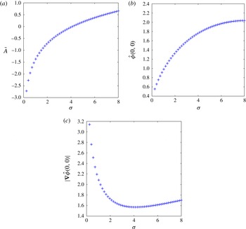
(a) Numerical approximations to the constant
 $\bar{A}$
, which appeared in (3.44), plotted against different values of
 ${\it\sigma}$
. (b) The value of
 $\hat{{\it\phi}}(0,0)$
together with the numerical approximation for
 $\hat{{\it\phi}}_{0}$
, from (3.44) (after making use of
 $\bar{A}$
). In this case no difference between
 $\hat{{\it\phi}}(0,0)$
and
 $\hat{{\it\phi}}_{0}$
, from (3.44), is observed. (c) Numerical approximations for
 $|\boldsymbol{{\rm\nabla}}\hat{{\it\phi}}(0,0)|$
plotted against
 ${\it\sigma}$
.

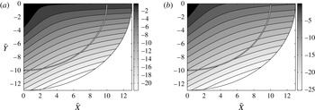
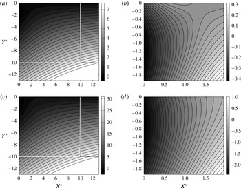
A contour plot of
 $\hat{{\it\phi}}$
. The thick line indicates the location
 $\bar{R}=10.0$
which demarcates the numerical solution (that is, the region inside
 $\bar{R}=10.0$
) and the far-field form (3.40): (a)
 ${\it\sigma}=1$
, (b)
 ${\it\sigma}=8$
.

We now perform a numerical solution of the harmonic boundary value problem (3.34)–(3.39) using finite differences. In doing so, the regularity condition (3.41) is enforced as
 $\bar{R}\rightarrow 0$
by using the near-field asymptotic form (3.42) and (3.44) to apply the near-field boundary condition
 $$\begin{eqnarray}\hat{{\it\phi}}_{\bar{{\it\theta}}}\sin \bar{{\it\theta}}-\bar{R}\cos \bar{{\it\theta}}\,\hat{{\it\phi}}_{\bar{R}}=\frac{{\rm\pi}}{2}\bar{R}\quad \text{on}~\bar{R}={\it\epsilon},-{\rm\pi}/2<\bar{{\it\theta}}<0,\end{eqnarray}$$
with
 ${\it\epsilon}>0$
chosen sufficiently small. We use finite differences in polar coordinates with a value of
 $R_{\infty }=25$
. Thereafter, the constant
 $\bar{A}$
in (3.44) can be approximated numerically. The results of these numerical approximations for
 $\bar{A}$
are shown in figure 3 for a range of values of
 ${\it\sigma}$
. We also plot the direct numerical approximations for
 $\hat{{\it\phi}}(0,0)$
against
 ${\it\sigma}$
along with the approximation obtained by using
 $\bar{A}$
in (3.44) to determine
 $\hat{{\it\phi}}_{0}$
. We find that there is no discernible difference between the two values. In figure 3 we plot
 $|\boldsymbol{{\rm\nabla}}\hat{{\it\phi}}(0,0)|$
against values of
 ${\it\sigma}$
. In figure 4 we show contour plots of
 $\hat{{\it\phi}}$
in the quarter-plane for two different values of
 ${\it\sigma}$
. In these plots we show a comparison between the numerical values of
 $\hat{{\it\phi}}$
obtained and the far-field form for
 $\hat{{\it\phi}}$
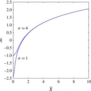
given by (3.40). In figure 5 we show plots of
 $\hat{{\it\eta}}$
for two different values of
 ${\it\sigma}$
. It is of interest to obtain the properties of the flow at the contact point. The expression for the contact point is
 $y_{p}(t)$
, and this is given, via (3.16), (3.18), (3.25), (3.27), (3.42) and (3.44), as
 $$\begin{eqnarray}y_{p}(t)=\frac{2{\it\sigma}}{{\rm\pi}}t^{2}(-\ln t)-\frac{{\it\sigma}}{{\rm\pi}}t^{2}\ln (-\ln t)-\frac{{\it\sigma}}{{\rm\pi}}(\bar{A}-1)t^{2}+o(t^{2}),\end{eqnarray}$$
as
 $t\rightarrow 0^{+}$
. The free surface slope at the contact point is given, via (3.16), (3.18), (3.25), (3.27), (3.42) and (3.44), by
 $$\begin{eqnarray}{\it\eta}_{\bar{x}}(0,t)=-\frac{{\rm\pi}}{4(-\ln t)}+o\left(\frac{1}{(-\ln t)}\right),\end{eqnarray}$$
as
 $t\rightarrow 0^{+}$
. Similarly, the fluid velocity at the contact point is given by
 $$\begin{eqnarray}\boldsymbol{{\rm\nabla}}{\it\phi}(0,y_{p}(t),t)={\it\sigma}t\,\boldsymbol{i}+\frac{2{\it\sigma}}{{\rm\pi}}[2t(-\ln t)-t(\ln (-\ln t))-\bar{A}t]\,\boldsymbol{j}+o(t),\end{eqnarray}$$
as
 $t\rightarrow 0^{+}$
. Finally, we consider the dynamic pressure in the inner region. It follows from (2.14) and (3.18) that the inner-region asymptotic expansion for the dynamic pressure takes the form
 $$\begin{eqnarray}p_{d}(X,Y,t)=-\frac{4{\it\sigma}}{{\rm\pi}}t^{2}(-\ln t)^{2}\left(Y-\frac{2{\it\sigma}}{{\rm\pi}}\right)+o(t^{2}(-\ln t)^{2}),\end{eqnarray}$$
as
 $t\rightarrow 0^{+}$
.
A plot of
 $\hat{{\it\eta}}$
for different
 ${\it\sigma}$
.

We next consider the structure of the solution to [IBVP] as
 $(\bar{x},y)\rightarrow (0,y_{p}(t))$
with
 $t=O(1)$
.
4. Asymptotic structure for [IBVP] as
$(\bar{x},y)\rightarrow (0,y_{p}(t))$
with
$t=O(1)$


In this section we consider the asymptotic structure of the solution to [IBVP] as
 $(\bar{x},y)\rightarrow (0,y_{p}(t))$
with
 $t=O(1)$
. We first write
 $$\begin{eqnarray}\displaystyle & {\it\eta}(\bar{x},t)={\it\eta}_{0}(t)+{\it\eta}_{1}(t)\bar{x}+o(\bar{x}), & \displaystyle\end{eqnarray}$$
 $$\begin{eqnarray}\displaystyle & {\it\phi}(\bar{x},y,t)={\it\phi}_{0}(t)+u_{0}(t)\bar{x}+v_{0}(t)(y-y_{p}(t))+o(\bar{x},(y-y_{p}(t))), & \displaystyle\end{eqnarray}$$
as
 $(\bar{x},y)\rightarrow (0,y_{p}(t))$
, where
 ${\it\phi}_{0}(t)={\it\phi}(0,y_{p}(t),t)$
,
 $u_{0}(t)={\it\phi}_{\bar{x}}(0,y_{p}(t),t)$
and
 $v_{0}(t)={\it\phi}_{y}(0,y_{p}(t),t)$
with
 ${\it\eta}_{0}(t)={\it\eta}(0,t)$
and
 ${\it\eta}_{1}(t)={\it\eta}_{\bar{x}}(0,t)$
. We now substitute from (4.1) and (4.2) into (2.4), (2.5), (2.7) and (2.8), recalling that
 $y_{p}(t)={\it\eta}(0,t)$
via (2.3). We obtain
 $$\begin{eqnarray}{\it\eta}_{0}(t)=y_{p}(t),\quad {\it\eta}_{1}(t)=\frac{-\ddot{s}(t)}{(1+\ddot{y} _{p}(t))},\quad u_{0}(t)={\dot{s}}(t),\end{eqnarray}$$
 $$\begin{eqnarray}v_{0}(t)={\dot{y}}_{p}(t),\quad \dot{{\it\phi}}_{0}(t)={\textstyle \frac{1}{2}}({\dot{s}}^{2}(t)+{\dot{y}}_{p}^{2}(t))-y_{p}(t),\end{eqnarray}$$
for
 $t>0$
. Specifically, via (4.1), (4.2) and (4.4) we have
 $$\begin{eqnarray}\boldsymbol{{\rm\nabla}}{\it\phi}(0,y_{p}(t),t)=({\dot{s}}(t),{\dot{y}}_{p}(t))\end{eqnarray}$$
and
 $$\begin{eqnarray}{\it\eta}_{\bar{x}}(0,t)=\frac{-\ddot{s}(t)}{(1+\ddot{y} _{p}(t))},\end{eqnarray}$$
for
 $t>0$
. In the above, an overdot represents differentiation with respect to
 $t$
. Recalling that
 $\ddot{s}(t)={\it\sigma}$
and from (3.46) that
 $\ddot{y} _{p}(t)\sim (4{\it\sigma}/{\rm\pi})(-\ln t)$
and
 ${\dot{y}}_{p}(t)\sim (4{\it\sigma}/{\rm\pi})t(-\ln t)$
as
 $t\rightarrow 0^{+}$
, it follows from (4.5) and (4.6) that
 $$\begin{eqnarray}\boldsymbol{{\rm\nabla}}{\it\phi}(0,y_{p}(t),t)\sim {\it\sigma}t\left(1,\frac{4}{{\rm\pi}}(-\ln t)\right),\quad {\it\eta}_{\bar{x}}(0,t)\sim -\frac{{\rm\pi}}{4(-\ln t)},\end{eqnarray}$$
as
 $t\rightarrow 0^{+}$
, which is in agreement with the direct calculation leading to (3.47) and (3.48). The results of this section will play a significant role throughout the remainder of this paper. We are now in a position to include the effects of weak surface tension in [IBVP].
5. The problem [IBVP] including surface tension
We are now in a position to consider the effects of introducing surface tension into the model for the interaction of a free surface with a uniformly accelerated vertical plate. The presence of surface tension leads to a modification of the boundary condition (2.8), with surface tension now balancing the pressure discontinuity across the free surface, so that Bernoulli’s equation at the free surface gives
 $$\begin{eqnarray}{\it\phi}_{t}-{\dot{s}}(t){\it\phi}_{\bar{x}}+\frac{1}{2}|\boldsymbol{{\rm\nabla}}{\it\phi}|^{2}+{\it\eta}=\mathscr{W}\frac{{\it\eta}_{\bar{x}\bar{x}}}{(1+{\it\eta}_{\bar{x}}^{2})^{3/2}},\quad y={\it\eta}(\bar{x},t),\bar{x}>0,t>0,\end{eqnarray}$$
where
 $\mathscr{W}$
is the dimensionless inverse Weber number given by
 $\mathscr{W}=T/{\it\rho}gh^{2}=(h_{T}/h)^{2}$
. Here
 $T$
is the coefficient of surface tension, whilst
 $h_{T}$
is the capillary length scale, which is typically 2 mm for water, and gives a measure of the meniscus length at the contact point.
The inclusion of surface tension into the model requires an additional boundary condition at the contact point between the plate and the free surface. We consider, as the simplest case, the situation where the specified contact angle between the plate and the free surface is
 ${\rm\pi}/2$
(although the approach developed here is readily adaptable to differing contact angles). The contact condition at the contact point is then
 $$\begin{eqnarray}{\it\eta}_{\bar{x}}(0,t,\mathscr{W})=0,\quad t\geqslant 0.\end{eqnarray}$$
The initial–boundary value problem [IBVP] that is modified to include surface tension and the contact condition (5.2) will be henceforth referred to as
 $[\text{IBVP}]^{\prime }$
. We consider
 $[\text{IBVP}]^{\prime }$
when the effects of surface tension are weak, so that
 $0<\mathscr{W}\ll 1$
, and develop the asymptotic structure to
 $[\text{IBVP}]^{\prime }$
as
 $\mathscr{W}\rightarrow 0$
via the method of matched asymptotic expansions.
5.1. Outer region (I) as
$\mathscr{W}\rightarrow 0$

We expand the potential and free surface function in the forms
 $$\begin{eqnarray}\displaystyle {\it\phi}(\bar{x},y,t;\mathscr{W}) & = & \displaystyle {\it\phi}_{0}(\bar{x},y,t)+o(1),\end{eqnarray}$$
 $$\begin{eqnarray}\displaystyle {\it\eta}(\bar{x},t;\mathscr{W}) & = & \displaystyle {\it\eta}_{0}(\bar{x},t)+o(1),\end{eqnarray}$$
 $\mathscr{W}\rightarrow 0$
, with
 $(\bar{x},y)\in \bar{D}(t)$
and
 $t=O(1)$
. We then substitute the expansions (5.3) and (5.4) into
 $[\text{IBVP}]^{\prime }$
. As may be anticipated, we find that the leading-order problem is given by [IBVP]. The structure of
 ${\it\phi}_{0}(\bar{x},y,t)$
and
 ${\it\eta}_{0}(\bar{x},t)$
as
 $t\rightarrow 0^{+}$
is given in §§ 3.1 and 3.2, uniformly for
 $(x,y)\in \bar{\mathscr{D}}(t)$
, and in § 4 as
 $(\bar{x},y)\rightarrow (0,y_{p}(t))$
, uniformly for
 $t\geqslant 0$
. Accordingly, for this leading-order problem, the contact point is located at
 $$\begin{eqnarray}(\bar{x},y)=(0,y_{0}(t)),\quad t\geqslant 0,\end{eqnarray}$$
with
 $y_{0}(t)={\it\eta}_{0}(0,t)$
. On using expressions (3.22), (3.35) and (3.44), we have that
 $$\begin{eqnarray}y_{0}(t)=\frac{2{\it\sigma}}{{\rm\pi}}t^{2}(-\ln t)-\frac{{\it\sigma}}{{\rm\pi}}t^{2}(\ln (-\ln t))+Kt^{2}+o(t^{2})\quad \text{as }t\rightarrow 0^{+},\end{eqnarray}$$
where
 $K$
is a constant that depends upon
 ${\it\sigma}$
and is given by (see King & Needham Reference King and Needham1994)
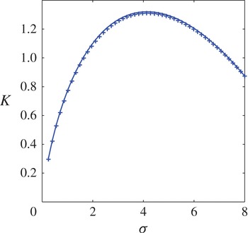
 $$\begin{eqnarray}K=\frac{{\it\sigma}}{{\rm\pi}}\left(\ln \frac{4}{{\it\sigma}}+1+\frac{{\it\Gamma}^{\prime }({\textstyle \frac{3}{2}})}{{\it\Gamma}({\textstyle \frac{3}{2}})}\right)=\frac{{\it\sigma}}{{\rm\pi}}(1-\bar{A}).\end{eqnarray}$$
A graph of
 $K$
against
 ${\it\sigma}$
is shown in figure 6. Numerical values of
 $K$
obtained from the numerical solution of § 3.2 are also shown.
A plot of
 $K$
against
 ${\it\sigma}$
from (5.7). The values of
 $K$
obtained from the numerical solution of the inner problem are also shown. The solid line refers to the numerical calculation for
 $K$
whilst the symbols denote the analytical expression for
 $K$
.

It follows from (5.6) that
 $$\begin{eqnarray}\ddot{y} _{0}(t)=\frac{4{\it\sigma}}{{\rm\pi}}(-\ln t)-\frac{2{\it\sigma}}{{\rm\pi}}\ln (-\ln t)+\left(2K-\frac{6{\it\sigma}}{{\rm\pi}}\right)+o(1)\quad \text{as }t\rightarrow 0^{+}.\end{eqnarray}$$
We therefore have from (4.6) that
 $$\begin{eqnarray}{\it\eta}_{0\bar{x}}(0,t)=\frac{-{\rm\pi}}{4(-\ln t)}+O\left(\frac{(\ln (-\ln t))}{(-\ln t)^{2}}\right)\quad \text{as }t\rightarrow 0^{+}.\end{eqnarray}$$
Now (5.9) does not satisfy the contact condition (5.2), which requires
 $$\begin{eqnarray}{\it\eta}_{0\bar{x}}(0,t)=0,\quad t\geqslant 0.\end{eqnarray}$$
We must conclude that expansions (5.3) and (5.4) become non-uniform when
 $(\bar{x},y)=(0,y_{0}(t))+o(1)$
as
 $\mathscr{W}\rightarrow 0$
with
 $t=O(1)$
. This necessitates the introduction of a local asymptotic region close to the contact point, where
 $(\bar{x},y)=(0,y_{0}(t))+o(1)$
as
 $\mathscr{W}\rightarrow 0$
with
 $t=O(1)$
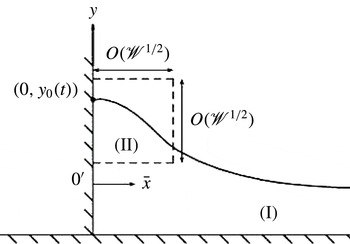
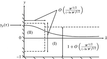
, through which the contact condition (5.10) is satisfied. We therefore require a second outer region (see figure 7) in which surface tension effects are retained at leading order. We refer to this localized region as outer region (II).
A sketch showing outer region (II) in which surface tension effects are retained.

5.2. Outer region (II) as
$\mathscr{W}\rightarrow 0$

We now consider outer region (II) close to the contact point (as deduced from outer region (I)) in which we must retain surface tension at leading order as
 $\mathscr{W}\rightarrow 0$
. We write
 $$\begin{eqnarray}\bar{x}=O(\mathscr{W}^{a}),\quad y=y_{0}(t)+O(\mathscr{W}^{a}).\end{eqnarray}$$
It then follows, via Van Dyke’s (Reference Van Dyke1975) matching principle and the outer-region (I) asymptotic expansions (5.3) and (5.4), together with the expressions from (4.4), that
 $$\begin{eqnarray}{\it\phi}={\it\phi}_{0}(t)+\mathscr{W}^{a}\left[\frac{u_{0}(t)\bar{x}}{\mathscr{W}^{a}}+\frac{v_{0}(t)(y-y_{0}(t))}{\mathscr{W}^{a}}\right]+O(\mathscr{W}^{b}),\quad {\it\eta}=y_{0}(t)+O(\mathscr{W}^{a}),\quad\end{eqnarray}$$
as
 $\mathscr{W}\rightarrow 0$
in outer region (II), with
 $b>a>0$
to be determined so that surface tension effects are introduced at leading order as
 $\mathscr{W}\rightarrow 0$
. An examination of the boundary condition (4.1) together with (5.11) and (5.12), with a view to retaining surface tension effects in a non-trivial balance, requires that
 $O(\mathscr{W}^{b-a})+O(\mathscr{W}^{a})\sim O(\mathscr{W}^{1-a})$
. This balance is achieved by choosing
 $a=1/2$
and
 $b=1$
. Thus, in outer region (II) we write
 $$\begin{eqnarray}\bar{x}=\mathscr{W}^{1/2}\tilde{x},\quad y=y_{0}(t)+\mathscr{W}^{1/2}{\tilde{y}},\end{eqnarray}$$
where
 $\tilde{x},{\tilde{y}},t=O(1)$
as
 $\mathscr{W}\rightarrow 0$
with
 $t=O(1)$
. We are now in a position to introduce the asymptotic expansions in outer region (II), via (5.12), as
 $$\begin{eqnarray}\displaystyle & {\it\eta}(\tilde{x},t,\mathscr{W})=y_{0}(t)+\mathscr{W}^{1/2}\tilde{{\it\eta}}(\tilde{x},t)+o(\mathscr{W}^{1/2}), & \displaystyle\end{eqnarray}$$
 $$\begin{eqnarray}\displaystyle & {\it\phi}(\tilde{x},{\tilde{y}},t,\mathscr{W})={\it\phi}_{0}(t)+\mathscr{W}^{1/2}[u_{0}(t)\tilde{x}+v_{0}(t){\tilde{y}}]+\mathscr{W}\tilde{{\it\phi}}(\tilde{x},{\tilde{y}},t)+o(\mathscr{W}), & \displaystyle\end{eqnarray}$$
 $\mathscr{W}\rightarrow 0$
with
 $(\tilde{x},{\tilde{y}})=O(1)$
and
 $t=O(1)$
. The free surface location in outer-region (II) coordinates is given by
 $$\begin{eqnarray}{\tilde{y}}=\tilde{{\it\eta}}(\tilde{x},t)+o(1),\end{eqnarray}$$
as
 $\mathscr{W}\rightarrow 0$
with
 $\tilde{x},t=O(1)$
. Next, after substitution of (5.13)–(5.16) into the full problem
 $[\text{IBVP}]^{\prime }$
, at leading order we obtain
 $$\begin{eqnarray}\displaystyle & (1+\tilde{{\it\eta}}_{\tilde{x}}^{2})^{-3/2}\tilde{{\it\eta}}_{\tilde{x}\tilde{x}}-(1+\ddot{y} _{0}(t))\tilde{{\it\eta}}=\ddot{s}(t)\tilde{x},\quad \tilde{x}>0,t>0, & \displaystyle\end{eqnarray}$$
 $$\begin{eqnarray}\displaystyle & \tilde{{\it\eta}}_{\tilde{x}}(0,t)=0,\quad t>0, & \displaystyle\end{eqnarray}$$
 $$\begin{eqnarray}\displaystyle & \displaystyle \tilde{{\it\eta}}(\tilde{x},t)\sim \frac{-\ddot{s}(t)\tilde{x}}{(1+\ddot{y} _{0}(t))},\quad \text{as}~\tilde{x}\rightarrow \infty ,t>0. & \displaystyle\end{eqnarray}$$
 $\tilde{{\it\eta}}(\tilde{x},t)$
, comprising (5.17)–(5.19), which we denote as [EVP], with the final boundary condition arising from matching to outer region (I), using (5.1), (5.13) and (5.15). We then have
 $$\begin{eqnarray}\displaystyle & \tilde{{\rm\nabla}}^{2}\tilde{{\it\phi}}=0,\quad \tilde{x}>0,-\infty <{\tilde{y}}<\tilde{{\it\eta}}(\tilde{x},t),t>0, & \displaystyle\end{eqnarray}$$
 $$\begin{eqnarray}\displaystyle & \tilde{{\it\phi}}_{\tilde{x}}=0,\quad \tilde{x}=0,-\infty <{\tilde{y}}<\tilde{{\it\eta}}(\tilde{x},t),t>0, & \displaystyle\end{eqnarray}$$
 $$\begin{eqnarray}\displaystyle & \tilde{{\it\eta}}_{t}+\tilde{{\it\phi}}_{\tilde{x}}\tilde{{\it\eta}}_{\tilde{x}}-\tilde{{\it\phi}}_{{\tilde{y}}}=0,\quad \tilde{x}>0,{\tilde{y}}=\tilde{{\it\eta}}(\tilde{x},t),t>0, & \displaystyle\end{eqnarray}$$
 $$\begin{eqnarray}\displaystyle & \tilde{{\it\phi}}(\tilde{x},{\tilde{y}},t)\sim {\it\delta}(t)(\tilde{x}^{2}-{\tilde{y}}^{2})\quad \text{as}~\tilde{x}\rightarrow \infty ,\text{for }-\infty <{\tilde{y}}\leqslant \tilde{{\it\eta}}(\tilde{x},t),t>0, & \displaystyle\end{eqnarray}$$
with appropriate regularity conditions at the contact point
 $(\tilde{x},{\tilde{y}})=(0,\tilde{{\it\eta}}(0,t))$
. Here,
 ${\it\delta}(t)=-\dot{{\it\gamma}}(t)/(4{\it\gamma}(t))$
and
 ${\it\gamma}(t)=\ddot{s}(t)/(1+\ddot{y} _{p}(t))$
for
 $t>0$
. We shall refer to this problem, (5.20)–(5.23), as [PVP]. In addition, we have initial conditions given by
 $$\begin{eqnarray}\displaystyle & & \displaystyle [\text{EVP}]\quad \tilde{{\it\eta}}(\tilde{x},0)=0,\quad \tilde{x}\geqslant 0,\end{eqnarray}$$
 $$\begin{eqnarray}\displaystyle & & \displaystyle [\text{PVP}]\quad \tilde{{\it\phi}}(\tilde{x},{\tilde{y}},0)=0,\quad \tilde{x}\geqslant 0,-\infty <{\tilde{y}}\leqslant 0.\end{eqnarray}$$
 $(\bar{x},y)\rightarrow (0,y_{0}(t))$
with
 $t=O(1)$
.
We now focus on [EVP]. In particular, we examine the structure of the solution to [EVP] for
 $0<t\ll 1$
. Using (5.6), with
 ${\it\sigma}>0$
, we may write [EVP], with
 $0<t\ll 1$
, in the form
 $$\begin{eqnarray}\displaystyle & \displaystyle (1+\tilde{{\it\eta}}_{\tilde{x}}^{2})^{-3/2}\tilde{{\it\eta}}_{\tilde{x}\tilde{x}}-\frac{{\it\sigma}}{{\rm\pi}}[4(-\ln t)+O(\ln (-\ln t))]\tilde{{\it\eta}}={\it\sigma}\tilde{x},\quad \tilde{x}>0,t>0, & \displaystyle\end{eqnarray}$$
 $$\begin{eqnarray}\displaystyle & \displaystyle \tilde{{\it\eta}}_{\tilde{x}}(0,t)=0,\quad t>0, & \displaystyle\end{eqnarray}$$
 $$\begin{eqnarray}\displaystyle & \displaystyle \tilde{{\it\eta}}(\tilde{x},t)\sim \frac{-{\rm\pi}\tilde{x}}{4(-\ln t)},\quad \text{as}~\tilde{x}\rightarrow \infty ,t>0. & \displaystyle\end{eqnarray}$$
 $\tilde{{\it\eta}}(\tilde{x},t)=o(1)$
for
 $0<t\ll 1$
with
 $\tilde{x}=O(1)$
. We therefore expand as
 $$\begin{eqnarray}\tilde{{\it\eta}}(\tilde{x},t)=\frac{\tilde{{\it\eta}}_{0}(\tilde{x})}{(-\ln t)}+o((-\ln t)^{-1})\quad \text{as }t\rightarrow 0^{+}~\text{with}~\tilde{x}=O(1),\end{eqnarray}$$
and after substitution into (5.26) and (5.28) we obtain
 $$\begin{eqnarray}\tilde{{\it\eta}}_{0}(\tilde{x})=-\frac{{\rm\pi}\tilde{x}}{4},\quad \tilde{x}>0,\end{eqnarray}$$
and so
 $$\begin{eqnarray}\tilde{{\it\eta}}(\tilde{x},t)=\frac{-{\rm\pi}\tilde{x}}{4(-\ln t)}+o\left(\frac{\tilde{x}}{(-\ln t)}\right)\quad \text{as}~t\rightarrow 0^{+}~\text{with}~\tilde{x}=O(1),\end{eqnarray}$$
with the initial condition (5.25) being satisfied. However, this expansion does not satisfy boundary condition (5.27) at
 $\tilde{x}=0$
. We therefore require a further region with
 $\tilde{x}=o(1)$
as
 $t\rightarrow 0^{+}$
. We write
 $\tilde{x}\sim {\it\psi}(t)$
where
 ${\it\psi}(t)=o(1)$
as
 $t\rightarrow 0^{+}$
. Then it follows from (5.31) that
 $\tilde{{\it\eta}}\sim {\it\psi}(t)/(-\ln t)$
, and thus in order to obtain a balance of terms in (5.26) we require
 ${\it\psi}(t)=(-\ln t)^{-1/2}$
. We therefore expand in the form
 $$\begin{eqnarray}\tilde{{\it\eta}}(\tilde{X},t)=\frac{1}{(-\ln t)^{3/2}}\tilde{{\it\eta}}_{0}(\tilde{X})+o((-\ln t)^{-3/2}),\end{eqnarray}$$
as
 $t\rightarrow 0^{+}$
with
 $\tilde{X}=O(1)$
. In the above, we have introduced the scaled variable
 $\tilde{X}=(-\ln t)^{1/2}\tilde{x}$
with
 $\tilde{X}=O(1)$
as
 $t\rightarrow 0^{+}$
. The leading-order problem is then given by
 $$\begin{eqnarray}\displaystyle & \displaystyle \tilde{{\it\eta}}_{0\tilde{X}\tilde{X}}-\frac{4{\it\sigma}}{{\rm\pi}}\tilde{{\it\eta}}_{0}={\it\sigma}\tilde{X},\quad \tilde{X}>0, & \displaystyle\end{eqnarray}$$
 $$\begin{eqnarray}\displaystyle & \tilde{{\it\eta}}_{0\tilde{X}}(0)=0, & \displaystyle\end{eqnarray}$$
 $$\begin{eqnarray}\displaystyle & \displaystyle \tilde{{\it\eta}}_{0}(\tilde{X})\sim -\frac{{\rm\pi}}{4}\tilde{X}\quad \text{as}~\tilde{X}\rightarrow \infty . & \displaystyle\end{eqnarray}$$
 $$\begin{eqnarray}\tilde{{\it\eta}}_{0}(\tilde{X})=A\text{e}^{{\it\lambda}\tilde{X}}+B\text{e}^{-{\it\lambda}\tilde{X}}-\frac{{\rm\pi}}{4}\tilde{X},\quad \tilde{X}\geqslant 0,\end{eqnarray}$$
with
 ${\it\lambda}=2\sqrt{{\it\sigma}/{\rm\pi}}$
and
 $A,B\in \mathbb{R}$
. Application of (5.35) requires
 $A=0$
, after which condition (5.34) requires
 $B=-{\rm\pi}^{3/2}/(8\sqrt{{\it\sigma}})$
, and hence we have
 $$\begin{eqnarray}\tilde{{\it\eta}}_{0}(\tilde{X})=-\frac{{\rm\pi}^{3/2}}{8\sqrt{{\it\sigma}}}\,\text{e}^{-{\it\lambda}\tilde{X}}-\frac{{\rm\pi}}{4}\tilde{X},\quad \tilde{X}\geqslant 0,\end{eqnarray}$$
and so from (5.32) we have
 $$\begin{eqnarray}\tilde{{\it\eta}}(\tilde{X},t)=\frac{1}{(-\ln t)^{3/2}}\left(-\frac{{\rm\pi}^{3/2}}{8\sqrt{{\it\sigma}}}\,\text{e}^{-{\it\lambda}\tilde{X}}-\frac{{\rm\pi}}{4}\tilde{X}\right)+o((-\ln t)^{-3/2}),\end{eqnarray}$$
as
 $t\rightarrow 0^{+}$
with
 $\tilde{X}=O(1)$
. We note that initial condition (5.25) is satisfied. Thus, for
 $0<t\ll 1$
, in outer region (II) we have
 $$\begin{eqnarray}\displaystyle {\it\eta}(\tilde{x},t;\mathscr{W}) & = & \displaystyle \left[\frac{2{\it\sigma}}{{\rm\pi}}t^{2}(-\ln t)-\frac{{\it\sigma}}{{\rm\pi}}t^{2}(\ln (-\ln t))+Kt^{2}+\cdots \,\right]\nonumber\\ \displaystyle & & \displaystyle +\,\mathscr{W}^{1/2}\left(\frac{-{\rm\pi}\tilde{x}}{(-\ln t)}+o((-\ln t)^{-1})\right)\quad \nonumber\\ \displaystyle & & \displaystyle \qquad \text{as}~\mathscr{W}\rightarrow 0,\text{with }0<t\ll 1~\text{and}~\tilde{x}=O(1)>0,\end{eqnarray}$$
and
 $$\begin{eqnarray}\displaystyle {\it\eta}(\tilde{X},t;\mathscr{W}) & = & \displaystyle \left[\frac{2{\it\sigma}}{{\rm\pi}}t^{2}(-\ln t)-\frac{{\it\sigma}}{{\rm\pi}}t^{2}(\ln (-\ln t))+Kt^{2}+\cdots \,\right]\nonumber\\ \displaystyle & & \displaystyle +\,\mathscr{W}^{1/2}\left[\frac{1}{(-\ln t)^{3/2}}\left(-\frac{{\rm\pi}^{3/2}}{8\sqrt{{\it\sigma}}}\,\text{e}^{-{\it\lambda}\tilde{X}}-\frac{{\rm\pi}}{4}\tilde{X}\right)+\cdots \,\right]+\cdots \nonumber\\ \displaystyle & & \displaystyle \qquad \text{as}~\mathscr{W}\rightarrow 0,\text{with }0<t\ll 1~\text{and}~\tilde{X}=O(1)>0,\end{eqnarray}$$
from which it follows that
 $$\begin{eqnarray}\displaystyle y_{p}(t)={\it\eta}(0,t,\mathscr{W}) & = & \displaystyle \left[\frac{2{\it\sigma}}{{\rm\pi}}t^{2}(-\ln t)-\frac{{\it\sigma}}{{\rm\pi}}t^{2}(\ln (-\ln t))+Kt^{2}+\cdots \,\right]\nonumber\\ \displaystyle & & \displaystyle -\,\mathscr{W}^{1/2}\left[\frac{1}{(-\ln t)^{3/2}}\frac{{\rm\pi}^{3/2}}{8\sqrt{{\it\sigma}}}+\cdots \,\right]+\cdots \nonumber\\ \displaystyle & & \displaystyle \qquad \text{as }\mathscr{W}\rightarrow 0,\text{with }0<t\ll 1.\end{eqnarray}$$
We observe from the structure of (5.40) that, in effect, outer region (II) has the spatial structure
 $\bar{x}\sim O(\mathscr{W}^{1/2}(-\ln t)^{-1/2})$
and so
 $y\sim ((2{\it\sigma}/{\rm\pi})t^{2}(-\ln t)+\cdots )+O(\mathscr{W}^{1/2}(-\ln t)^{-1/2})$
as
 $t\rightarrow 0^{+}$
. We now examine [PVP] as
 $t\rightarrow 0^{+}$
. It follows that
 ${\it\delta}(t)\sim 1/(4t(-\ln t))$
as
 $t\rightarrow 0^{+}$
. Thus, when
 $\tilde{x},{\tilde{y}}=O(1)$
as
 $t\rightarrow 0^{+}$
, we must expand in the form
 $$\begin{eqnarray}\tilde{{\it\phi}}(\tilde{x},{\tilde{y}},t)=\frac{1}{4t(-\ln t)}\tilde{{\it\phi}}_{0}(\tilde{x},{\tilde{y}})+o\left(\frac{1}{t\ln t}\right)\quad \text{as }t\rightarrow 0^{+},\text{with}~\tilde{x},{\tilde{y}}=O(1).\end{eqnarray}$$
On substitution from (5.42) and (5.31) into (5.20)–(5.23), it is readily established that the leading-order problem has the unique solution
 $$\begin{eqnarray}\tilde{{\it\phi}}_{0}(\tilde{x},{\tilde{y}})=\tilde{x}^{2}-{\tilde{y}}^{2},\quad \tilde{x}\geqslant 0,-\infty <{\tilde{y}}\leqslant 0.\end{eqnarray}$$
This structure will change when
 $\tilde{x},{\tilde{y}}=O((-\ln t)^{-1/2})$
as
 $t\rightarrow 0^{+}$
, driven by the change in the structure in
 $\tilde{{\it\eta}}$
. Introducing
 ${\tilde{Y}}=(-\ln t)^{1/2}{\tilde{y}}$
, then we expand as
 $$\begin{eqnarray}\tilde{{\it\phi}}(\tilde{X},{\tilde{Y}},t)=\frac{1}{4t(-\ln t)^{2}}\tilde{{\it\phi}}_{0}(\tilde{X},{\tilde{Y}})+o\left(\frac{1}{t(-\ln t)^{2}}\right)\quad \text{as }t\rightarrow 0^{+}~\text{with}~\tilde{X},{\tilde{Y}}=O(1).\quad\end{eqnarray}$$
The leading-order problem for
 $\tilde{{\it\phi}}_{0}(\tilde{X},{\tilde{Y}})$
is then given by
 $$\begin{eqnarray}\displaystyle & \tilde{\boldsymbol{{\rm\nabla}}}\tilde{{\it\phi}}_{0}=0,\quad \tilde{X}>0,-\infty <{\tilde{Y}}<0, & \displaystyle\end{eqnarray}$$
 $$\begin{eqnarray}\displaystyle & \tilde{{\it\phi}}_{0\tilde{X}}=0,\quad \tilde{X}=0,-\infty <{\tilde{Y}}<0, & \displaystyle\end{eqnarray}$$
 $$\begin{eqnarray}\displaystyle & \tilde{{\it\phi}}_{0{\tilde{Y}}}=0,\quad \tilde{X}>0,{\tilde{Y}}=0, & \displaystyle\end{eqnarray}$$
 $$\begin{eqnarray}\displaystyle & \tilde{{\it\phi}}_{0}(\tilde{X},{\tilde{Y}})\sim (\tilde{X}^{2}-{\tilde{Y}}^{2})\quad \text{as}~\tilde{X}\rightarrow \infty ~\text{with }-\infty <{\tilde{Y}}\leqslant 0, & \displaystyle\end{eqnarray}$$
 $\tilde{{\it\phi}}_{0}\in C^{1}([0,\infty )\times (-\infty ,0])\cap C^{2}((0,\infty )\times (-\infty ,0))$
.
The solution to this boundary value problem is
 $$\begin{eqnarray}\tilde{{\it\phi}}_{0}(\tilde{X},{\tilde{Y}})=\tilde{X}^{2}-{\tilde{Y}}^{2},\quad \tilde{X}\geqslant 0,-\infty <{\tilde{Y}}\leqslant 0,\end{eqnarray}$$
and so from (5.44) we have
 $$\begin{eqnarray}\tilde{{\it\phi}}(\tilde{X},{\tilde{Y}},t)=\frac{(\tilde{X}^{2}-{\tilde{Y}}^{2})}{4t(-\ln t)^{2}}+o\left(\frac{1}{t(-\ln t)^{2}}\right)\quad \text{as}~t\rightarrow 0^{+}~\text{with}~\tilde{X},{\tilde{Y}}=O(1).\end{eqnarray}$$
We can therefore write out the full expression for
 ${\it\phi}$
as
 $$\begin{eqnarray}\displaystyle {\it\phi}(\tilde{x},{\tilde{y}},t;\mathscr{W}) & = & \displaystyle \left[t^{3}(\ln t)^{2}\frac{8{\it\sigma}^{2}}{3{\rm\pi}^{2}}-t^{3}(-\ln t)(\ln (-\ln t))\frac{8{\it\sigma}^{2}}{3{\rm\pi}^{2}}\right.\nonumber\\ \displaystyle & & \displaystyle \left.+\,t^{3}(-\ln t)\left(\frac{4{\it\sigma}K}{{\rm\pi}}-\frac{2{\it\sigma}}{{\rm\pi}}\hat{{\it\phi}}_{0}\right)\right]+\mathscr{W}^{1/2}\left[\frac{4{\it\sigma}}{{\rm\pi}}t(-\ln t){\tilde{y}}+{\it\sigma}t\tilde{x}+\cdots \,\right]\nonumber\\ \displaystyle & & \displaystyle +\,\mathscr{W}\left[\frac{1}{t(-\ln t)}\frac{(\tilde{x}^{2}-{\tilde{y}}^{2})}{4}+\cdots \,\right]+\cdots \nonumber\\ \displaystyle & & \displaystyle \qquad \text{as}~\mathscr{W}\rightarrow 0,\text{with}~0<t\ll 1~\text{and}~\tilde{x},(-{\tilde{y}})=O(1)({\geqslant}0),\end{eqnarray}$$
and
 $$\begin{eqnarray}\displaystyle {\it\phi}(\tilde{X},{\tilde{Y}},t;\mathscr{W}) & = & \displaystyle \left[t^{3}(\ln t)^{2}\frac{8{\it\sigma}^{2}}{3{\rm\pi}^{2}}-t^{3}(-\ln t)(\ln (-\ln t))\frac{8{\it\sigma}^{2}}{3{\rm\pi}^{2}}\right.\nonumber\\ \displaystyle & & \displaystyle \left.+\,t^{3}(-\ln t)\left(\frac{4{\it\sigma}K}{{\rm\pi}}-\frac{2{\it\sigma}}{{\rm\pi}}\hat{{\it\phi}}_{0}\right)\right]+\mathscr{W}^{1/2}\left[\frac{4{\it\sigma}}{{\rm\pi}}t(-\ln t)^{1/2}{\tilde{Y}}\right.\nonumber\\ \displaystyle & & \displaystyle \left.+\,{\it\sigma}t(-\ln t)^{-1/2}\tilde{X}+\cdots \right]+\mathscr{W}\left[\frac{1}{t(-\ln t)^{2}}\frac{(\tilde{X}^{2}-{\tilde{Y}}^{2})}{4}+\cdots \,\right]+\cdots \nonumber\\ \displaystyle & & \displaystyle \qquad \text{as}~\mathscr{W}\rightarrow 0,\text{with}~0<t\ll 1~\text{and}~\tilde{X},(-{\tilde{Y}})=O(1)({\geqslant}0),\end{eqnarray}$$
 $\hat{{\it\phi}}_{0}$
is given via (3.44) and (5.7). We observe from (5.52) that the initial condition (5.25) fails to be satisfied. In particular, an examination of (5.40), (5.41) and (5.52) reveals that in outer region (II) we have a non-uniformity when
 $t=o(1)$
and
 $\tilde{X},{\tilde{Y}}=O(1)$
as
 $\mathscr{W}\rightarrow 0$
. Specifically, this non-uniformity occurs when
 $t=O({\it\mu}(\mathscr{W}))$
as
 $\mathscr{W}\rightarrow 0$
, with
 ${\it\mu}(\mathscr{W})=o(1)$
as
 $\mathscr{W}\rightarrow 0$
, and
 $\bar{x},y=O(\mathscr{W}^{1/2}(-\ln {\it\mu}(\mathscr{W}))^{-1/2})$
as
 $\mathscr{W}\rightarrow 0$
. It then follows from (5.37) that
 ${\it\eta}=O({\it\mu}^{2}(\mathscr{W})[-\ln ({\it\mu}(\mathscr{W}))])$
as
 $\mathscr{W}\rightarrow 0$
. To capture the free surface, we require that
 ${\it\mu}^{2}(\mathscr{W})(-\ln {\it\mu}(\mathscr{W}))=O(\mathscr{W}^{1/2}(-\ln {\it\mu}(\mathscr{W}))^{-1/2})$
, as
 $\mathscr{W}\rightarrow 0$
, and hence we may take, without loss of generality,
 $$\begin{eqnarray}{\it\mu}(\mathscr{W})=\frac{\mathscr{W}^{1/4}}{(-\ln \mathscr{W})^{3/4}}.\end{eqnarray}$$
Thus, to complete the asymptotic structure for
 $[\text{IBVP}]^{\prime }$
as
 $\mathscr{W}\rightarrow 0$
we require two inner regions when
 $t=O(\mathscr{W}^{1/4}(-\ln \mathscr{W})^{-3/4})$
as
 $\mathscr{W}\rightarrow 0$
, namely, the following.
Inner region (I). In this region
 $\bar{x},y=O(1)$
and
 $$\begin{eqnarray}{\it\eta}=O\left(\frac{\mathscr{W}^{1/2}}{(-\ln \mathscr{W})^{3/2}}\right),\quad {\it\phi}=O\left(\frac{\mathscr{W}^{1/4}}{(-\ln \mathscr{W})^{3/4}}\right),\end{eqnarray}$$
as
 $\mathscr{W}\rightarrow 0$
, via asymptotic expansions (5.3) and (5.4) in outer region (I), and the structure of the leading-order terms in (5.3) and (5.4) as
 $t\rightarrow 0^{+}$
with
 $\bar{x},y=O(1)$
(as given in § 3).
Inner region (II). In this region
 $\bar{x},y=O(\mathscr{W}^{1/2}(-\ln \mathscr{W})^{-1/2})$
and
 $$\begin{eqnarray}{\it\eta}=O\left(\frac{\mathscr{W}^{1/2}}{(-\ln \mathscr{W})^{1/2}}\right),\quad {\it\phi}=O\left(\frac{\mathscr{W}^{3/4}}{(-\ln \mathscr{W})^{1/4}}\right),\end{eqnarray}$$
as
 $\mathscr{W}\rightarrow 0$
, via asymptotic expansions (5.40) and (5.52) in outer region (II).
We now address inner region (I) and inner region (II) in detail.
5.3. Inner region (I)
We begin with inner region (I), where we introduce the inner coordinate
 ${\it\tau}$
via
 $$\begin{eqnarray}t=\mathscr{W}^{1/4}(-\ln \mathscr{W})^{-3/4}{\it\tau},\end{eqnarray}$$
with
 $\bar{x},y,{\it\tau}=O(1)$
as
 $\mathscr{W}\rightarrow 0$
in this region. It follows from (5.54) that asymptotic expansions in this region have the form
 $$\begin{eqnarray}\displaystyle {\it\phi}(\bar{x},y,{\it\tau};\mathscr{W}) & = & \displaystyle \mathscr{W}^{1/4}(-\ln \mathscr{W})^{-3/4}{\it\Phi}^{\curlyvee }(\bar{x},y,{\it\tau})+o(\mathscr{W}^{1/4}(-\ln \mathscr{W})^{-3/4}),\end{eqnarray}$$
 $$\begin{eqnarray}\displaystyle {\it\eta}(\bar{x},{\it\tau};\mathscr{W}) & = & \displaystyle \mathscr{W}^{1/2}(-\ln \mathscr{W})^{-3/2}{\it\eta}^{\curlyvee }(\bar{x},{\it\tau})+o(\mathscr{W}^{1/2}(-\ln \mathscr{W})^{-3/2}),\end{eqnarray}$$
 $\mathscr{W}\rightarrow 0$
uniformly in inner region (I). Substitution into the full problem
 $[\text{IBVP}]^{\prime }$
gives
 $$\begin{eqnarray}\displaystyle & {\rm\nabla}^{2}{\it\Phi}^{\curlyvee }=0,\quad (\bar{x},y)\in \mathscr{D}(0),{\it\tau}>0, & \displaystyle\end{eqnarray}$$
 $$\begin{eqnarray}\displaystyle & {\it\Phi}_{\bar{x}}^{\curlyvee }={\it\sigma}{\it\tau},\quad \bar{x}=0,-1<y<0,{\it\tau}>0, & \displaystyle\end{eqnarray}$$
 $$\begin{eqnarray}\displaystyle & {\it\eta}_{{\it\tau}}^{\curlyvee }-{\it\Phi}_{y}^{\curlyvee }=0,\quad y=0,\bar{x}>0,{\it\tau}>0, & \displaystyle\end{eqnarray}$$
 $$\begin{eqnarray}\displaystyle & {\it\Phi}_{{\it\tau}}^{\curlyvee }=0,\quad y=0,\bar{x}>0,{\it\tau}>0, & \displaystyle\end{eqnarray}$$
 $$\begin{eqnarray}\displaystyle & |\boldsymbol{{\rm\nabla}}{\it\Phi}^{\curlyvee }|\rightarrow 0\quad \text{as}~\bar{x}\rightarrow \infty ,\text{uniformly in }y\in [0,-1],{\it\tau}>0, & \displaystyle\end{eqnarray}$$
 $$\begin{eqnarray}\displaystyle & {\it\eta}^{\curlyvee }\rightarrow 0\quad \text{as}~\bar{x}\rightarrow \infty ,{\it\tau}>0. & \displaystyle\end{eqnarray}$$
 $|\boldsymbol{{\rm\nabla}}{\it\Phi}^{\curlyvee }|$
at
 $(\bar{x},y)=(0,0)$
and in
 ${\it\eta}^{\curlyvee }$
at
 $\bar{x}=0$
. We also have the initial conditions
 $$\begin{eqnarray}{\it\eta}^{\curlyvee }(\bar{x},0)=0,\bar{x}\geqslant 0,\quad {\it\Phi}^{\curlyvee }(\bar{x},y,0)=0,(\bar{x},y)\in \bar{\mathscr{D}}(0).\end{eqnarray}$$
We now write
 $$\begin{eqnarray}\displaystyle & {\it\eta}^{\curlyvee }(\bar{x},{\it\tau})={\it\tau}^{2}\tilde{{\it\eta}}^{\curlyvee }(\bar{x}),\quad \bar{x}\geqslant 0,{\it\tau}\geqslant 0, & \displaystyle\end{eqnarray}$$
 $$\begin{eqnarray}\displaystyle & {\it\Phi}^{\curlyvee }(\bar{x},y,{\it\tau})={\it\sigma}{\it\tau}\tilde{{\it\Phi}}^{\curlyvee }(\bar{x},y),\quad (\bar{x},y)\in \bar{\mathscr{D}}(0),{\it\tau}\geqslant 0. & \displaystyle\end{eqnarray}$$
 $\tilde{{\it\Phi}}^{\curlyvee }$
is then given by
 $$\begin{eqnarray}\displaystyle & {\rm\nabla}^{2}\tilde{{\it\Phi}}^{\curlyvee }=0,\quad (\bar{x},y)\in \mathscr{D}(0), & \displaystyle\end{eqnarray}$$
 $$\begin{eqnarray}\displaystyle & {\tilde{{\it\Phi}}^{\curlyvee }}_{\bar{x}}=1,\quad \bar{x}=0,-1<y<0, & \displaystyle\end{eqnarray}$$
 $$\begin{eqnarray}\displaystyle & {\tilde{{\it\Phi}}^{\curlyvee }}_{y}=0,\quad y=-1,\bar{x}>0, & \displaystyle\end{eqnarray}$$
 $$\begin{eqnarray}\displaystyle & \tilde{{\it\Phi}}^{\curlyvee }=0,\quad y=0,\bar{x}>0, & \displaystyle\end{eqnarray}$$
 $$\begin{eqnarray}\displaystyle & |\boldsymbol{{\rm\nabla}}\tilde{{\it\Phi}}^{\curlyvee }|\rightarrow 0\quad \text{as}~\bar{x}\rightarrow \infty ,\text{uniformly for }-1\leqslant y\leqslant 0, & \displaystyle\end{eqnarray}$$
 $|\boldsymbol{{\rm\nabla}}\tilde{{\it\Phi}}^{\curlyvee }|$
at
 $(\bar{x},y)=(0,0)$
. We then have
 $$\begin{eqnarray}\tilde{{\it\eta}}^{\curlyvee }(\bar{x})=\frac{{\it\sigma}}{2}{\tilde{{\it\Phi}}^{\curlyvee }}_{y}(\bar{x},0),\quad \bar{x}\geqslant 0.\end{eqnarray}$$
The (unique) solution to the harmonic boundary value problem has been obtained in § 3.1 as
 $$\begin{eqnarray}\tilde{{\it\Phi}}^{\curlyvee }(\bar{x},y)=\frac{8}{{\rm\pi}^{2}}\mathop{\sum }_{n=0}^{\infty }\frac{1}{(2n+1)^{2}}\,\text{e}^{-(n+1/2){\rm\pi}\bar{x}}\sin \left[\left(n+\frac{1}{2}\right)\!{\rm\pi}y\right],\quad (\bar{x},y)\in \bar{\mathscr{D}}(0)\setminus \{(0,0)\}\end{eqnarray}$$
with, via (5.73),
 $$\begin{eqnarray}\tilde{{\it\eta}}^{\curlyvee }(\bar{x})=\frac{2{\it\sigma}}{{\rm\pi}}\mathop{\sum }_{n=0}^{\infty }\frac{1}{(2n+1)}\,\text{e}^{-(n+1/2){\rm\pi}\bar{x}}=\frac{{\it\sigma}}{{\rm\pi}}\ln \left(\coth \left(\frac{{\rm\pi}\bar{x}}{4}\right)\right),\quad \bar{x}>0.\end{eqnarray}$$
Moreover, we recall, via (3.14) and (3.11), that
 $$\begin{eqnarray}\displaystyle \tilde{{\it\Phi}}^{\curlyvee }(r,{\it\theta}) & = & \displaystyle -\frac{2}{{\rm\pi}}(r\ln r)\sin {\it\theta}+\frac{2r}{{\rm\pi}}\left(1+\ln \left(\frac{4}{{\rm\pi}}\right)\right)\sin {\it\theta}-\frac{2r}{{\rm\pi}}{\it\theta}\cos {\it\theta}+O(r^{3}),\quad \nonumber\\ \displaystyle & & \displaystyle \text{as}~r\rightarrow 0,-{\rm\pi}/2\leqslant {\it\theta}\leqslant 0,\end{eqnarray}$$
and
 $$\begin{eqnarray}\tilde{{\it\eta}}^{\curlyvee }(\bar{x})=-\frac{{\it\sigma}}{{\rm\pi}}\ln \bar{x}+\frac{{\it\sigma}}{{\rm\pi}}\ln \left(\frac{4}{{\rm\pi}}\right)+O(\bar{x}^{2}),\quad \text{as}~\bar{x}\rightarrow 0,\end{eqnarray}$$
where
 $\bar{x}=r\cos {\it\theta}$
and
 $y=r\sin {\it\theta}$
.
Note that asymptotic matching of inner-region (I) expansions (5.58) (as
 ${\it\tau}\rightarrow \infty$
;
 $\bar{x},y=O(1)$
) with outer-region (I) expansions (5.3) and (5.4) (as
 $t\rightarrow 0^{+}$
;
 $\bar{x},y=O(1)$
) is readily verified. Also, observe that surface tension effects are not present at leading order in this region and hence the contact angle condition is not satisfied in this region. This is accommodated in inner region (II), which we now consider.
5.4. Inner region (II)
We next proceed to inner region (II), where we introduce the appropriate inner coordinates as
 $$\begin{eqnarray}t=\mathscr{W}^{1/4}(-\ln \mathscr{W})^{-3/4}{\it\tau},\quad \bar{x}=\mathscr{W}^{1/2}(-\ln \mathscr{W})^{-1/2}\hat{X},\quad y=\mathscr{W}^{1/2}(-\ln \mathscr{W})^{-1/2}{\hat{Y}},\end{eqnarray}$$
with
 $\hat{X},{\hat{Y}},{\it\tau}=O(1)$
as
 $\mathscr{W}\rightarrow 0$
. The asymptotic expansions for
 ${\it\phi}$
and
 ${\it\eta}$
are, via (5.15),
 $$\begin{eqnarray}\displaystyle {\it\phi}(\hat{X},{\hat{Y}},{\it\tau};\mathscr{W}) & = & \displaystyle \frac{\mathscr{W}^{3/4}}{(-\ln \mathscr{W})^{1/4}}\widehat{{\it\Phi}}_{0}(\hat{X},{\hat{Y}},{\it\tau})+\frac{\mathscr{W}^{3/4}\ln (-\ln \mathscr{W})}{(-\ln \mathscr{W})^{5/4}}\widehat{{\it\Phi}}_{1}(\hat{X},{\hat{Y}},{\it\tau})\nonumber\\ \displaystyle & & \displaystyle +\,\frac{\mathscr{W}^{3/4}}{(-\ln \mathscr{W})^{5/4}}\widehat{{\it\Phi}}_{2}(\hat{X},{\hat{Y}},{\it\tau})+o(\mathscr{W}^{3/4}(-\ln \mathscr{W})^{-5/4}),\end{eqnarray}$$
 $$\begin{eqnarray}\displaystyle {\it\eta}(\hat{X},{\it\tau};\mathscr{W}) & = & \displaystyle \frac{\mathscr{W}^{1/2}}{(-\ln \mathscr{W})^{1/2}}\widehat{{\it\eta}}_{0}(\hat{X},{\it\tau})+\frac{\mathscr{W}^{1/2}\ln (-\ln \mathscr{W})}{(-\ln \mathscr{W})^{3/2}}\widehat{{\it\eta}}_{1}(\hat{X},{\it\tau})\nonumber\\ \displaystyle & & \displaystyle +\,\frac{\mathscr{W}^{1/2}}{(-\ln \mathscr{W})^{3/2}}\widehat{{\it\eta}}_{2}(\hat{X},{\it\tau})+o(\mathscr{W}^{1/2}(-\ln \mathscr{W})^{-3/2}),\end{eqnarray}$$
 $\mathscr{W}\rightarrow 0$
in inner region (II). We note that the free surface location in this region is given by
 $$\begin{eqnarray}{\hat{Y}}=\hat{{\it\eta}}_{0}(\hat{X},{\it\tau})+\frac{\ln (-\!\ln \mathscr{W})}{(-\ln \mathscr{W})}\hat{{\it\eta}}_{1}(\hat{X},{\it\tau})+\frac{1}{(-\ln \mathscr{W})}\hat{{\it\eta}}_{2}(\hat{X},{\it\tau})+o((-\ln \mathscr{W})^{-1}),\quad \hat{X}\geqslant 0,{\it\tau}\geqslant 0,\end{eqnarray}$$
and
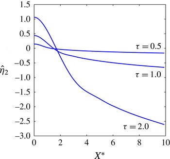
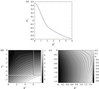
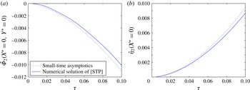
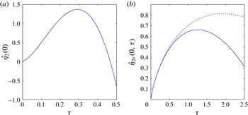
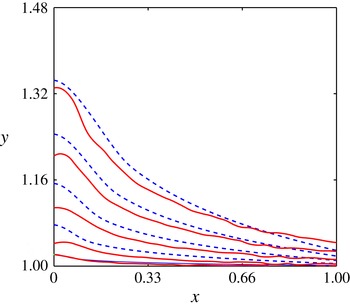
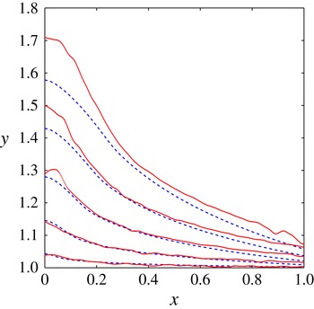
 $$\begin{eqnarray}\displaystyle y_{p}({\it\tau})={\it\eta}(0,{\it\tau},\mathscr{W}) & = & \displaystyle \frac{\mathscr{W}^{1/2}}{(-\ln \mathscr{W})^{1/2}}\hat{{\it\eta}}_{0}(0,{\it\tau})+\frac{\mathscr{W}^{1/2}\ln (-\ln \mathscr{W})}{(-\ln \mathscr{W})^{3/2}}\hat{{\it\eta}}_{1}(0,{\it\tau})\nonumber\\ \displaystyle & & \displaystyle +\,\frac{\mathscr{W}^{1/2}}{(-\ln \mathscr{W})^{3/2}}\hat{{\it\eta}}_{2}(0,{\it\tau})+o(\mathscr{W}^{1/2}(-\ln \mathscr{W})^{-3/2}).\end{eqnarray}$$
After substitution into the full problem
 $[\text{IBVP}]^{\prime }$
we obtain the leading-order problem as
 $$\begin{eqnarray}\displaystyle & {\rm\nabla}^{2}\widehat{{\it\Phi}}_{0}=0,\quad \hat{X}>0,-\infty <{\hat{Y}}<\hat{{\it\eta}}_{0}(\hat{X},{\it\tau}),{\it\tau}>0, & \displaystyle\end{eqnarray}$$
 $$\begin{eqnarray}\displaystyle & \widehat{{\it\Phi}}_{0\hat{X}}=0,\quad \hat{X}=0,-\infty <{\hat{Y}}<\hat{{\it\eta}}_{0}(0,{\it\tau}),{\it\tau}>0, & \displaystyle\end{eqnarray}$$
 $$\begin{eqnarray}\displaystyle & \hat{{\it\eta}}_{0{\it\tau}}-\hat{{\it\eta}}_{0\hat{X}}\widehat{{\it\Phi}}_{0\hat{X}}-\widehat{{\it\Phi}}_{0{\hat{Y}}}=0,\quad {\hat{Y}}=\hat{{\it\eta}}_{0}(\hat{X},{\it\tau}),\hat{X}>0, & \displaystyle\end{eqnarray}$$
 $$\begin{eqnarray}\displaystyle & \displaystyle \widehat{{\it\Phi}}_{0{\it\tau}}+\frac{1}{2}(\widehat{{\it\Phi}}_{0\hat{X}}^{2}+\widehat{{\it\Phi}}_{0{\hat{Y}}}^{2})=\frac{\hat{{\it\eta}}_{0\hat{X}\hat{X}}}{(1+\hat{{\it\eta}}_{0\hat{X}}^{2})^{3/2}},\quad {\hat{Y}}=\hat{{\it\eta}}_{0}(\hat{X},{\it\tau}),\hat{X}>0. & \displaystyle\end{eqnarray}$$
 $$\begin{eqnarray}\hat{{\it\eta}}_{0\hat{X}}(0,{\it\tau})=0,\quad {\it\tau}>0,\end{eqnarray}$$
with the initial conditions being
 $$\begin{eqnarray}\widehat{{\it\Phi}}_{0}(\hat{X},{\hat{Y}},0)=0,\quad \hat{X}\geqslant 0,-\infty <{\hat{Y}}\leqslant 0,\quad \hat{{\it\eta}}_{0}(\hat{X},0)=0,\quad \hat{X}\geqslant 0.\end{eqnarray}$$
We now require matching conditions to inner region (I). We must have
 $$\begin{eqnarray}\displaystyle & \displaystyle \widehat{{\it\Phi}}_{0}(\hat{X},{\hat{Y}},{\it\tau})=\frac{{\it\sigma}{\it\tau}}{{\rm\pi}}\hat{R}\sin {\it\theta}+o(\hat{R}),\quad \hat{R}\rightarrow \infty ,-{\rm\pi}/2\leqslant {\it\theta}\leqslant 0,{\it\tau}>0, & \displaystyle\end{eqnarray}$$
 $$\begin{eqnarray}\displaystyle & \displaystyle \hat{{\it\eta}}_{0}(\hat{X},{\it\tau})=\frac{{\it\sigma}{\it\tau}^{2}}{2{\rm\pi}}+o(1),\quad \hat{X}\rightarrow \infty ,{\it\tau}>0, & \displaystyle\end{eqnarray}$$
 $\hat{X}=\hat{R}\cos {\it\theta}$
and
 ${\hat{Y}}=\hat{R}\sin {\it\theta}$
. The problem for
 $\hat{{\it\Phi}}_{0}$
and
 $\hat{{\it\eta}}_{0}$
is now complete.
Note that surface tension effects are present in this leading-order problem. The simple form of the matching conditions allows us to write the solution as
 $$\begin{eqnarray}\displaystyle & \displaystyle \widehat{{\it\Phi}}_{0}(\hat{X},{\hat{Y}},{\it\tau})=\frac{{\it\sigma}{\it\tau}}{{\rm\pi}}{\hat{Y}}-\frac{{\it\sigma}^{2}{\it\tau}^{3}}{3{\rm\pi}^{2}},\quad \hat{X}\geqslant 0,-\infty \leqslant {\hat{Y}}\leqslant \frac{{\it\sigma}{\it\tau}^{2}}{2{\rm\pi}},{\it\tau}\geqslant 0, & \displaystyle\end{eqnarray}$$
 $$\begin{eqnarray}\displaystyle & \displaystyle \hat{{\it\eta}}_{0}(\hat{X},{\it\tau})=\frac{{\it\sigma}{\it\tau}^{2}}{2{\rm\pi}},\quad \hat{X}\geqslant 0,{\it\tau}\geqslant 0. & \displaystyle\end{eqnarray}$$
 $$\begin{eqnarray}\displaystyle & \displaystyle {\rm\nabla}^{2}\widehat{{\it\Phi}}_{1}=0,\quad \hat{X}>0,-\infty <{\hat{Y}}<\frac{{\it\sigma}{\it\tau}^{2}}{2{\rm\pi}},{\it\tau}>0, & \displaystyle\end{eqnarray}$$
 $$\begin{eqnarray}\displaystyle & \displaystyle \widehat{{\it\Phi}}_{1\hat{X}}=0,\quad \hat{X}=0,-\infty <{\hat{Y}}<\frac{{\it\sigma}{\it\tau}^{2}}{2{\rm\pi}},{\it\tau}>0, & \displaystyle\end{eqnarray}$$
 $$\begin{eqnarray}\displaystyle & \displaystyle \hat{{\it\eta}}_{1{\it\tau}}-\widehat{{\it\Phi}}_{1{\hat{Y}}}=0,\quad {\hat{Y}}=\frac{{\it\sigma}{\it\tau}^{2}}{2{\rm\pi}},\hat{X}>0,{\it\tau}>0, & \displaystyle\end{eqnarray}$$
 $$\begin{eqnarray}\displaystyle & \displaystyle \widehat{{\it\Phi}}_{1{\it\tau}}+\frac{{\it\sigma}}{{\rm\pi}}\hat{{\it\eta}}_{1}+\widehat{{\it\Phi}}_{0{\hat{Y}}}\widehat{{\it\Phi}}_{1{\hat{Y}}}=\hat{{\it\eta}}_{1\hat{X}\hat{X}},\quad {\hat{Y}}=\frac{{\it\sigma}{\it\tau}^{2}}{2{\rm\pi}},\hat{X}>0,{\it\tau}>0. & \displaystyle\end{eqnarray}$$
 $$\begin{eqnarray}\hat{{\it\eta}}_{1\hat{X}}(0,{\it\tau})=0,\quad {\it\tau}>0,\end{eqnarray}$$
whilst the initial conditions require
 $$\begin{eqnarray}\widehat{{\it\Phi}}_{1}(\hat{X},{\hat{Y}},0)=0,\quad \hat{X}\geqslant 0,-\infty <{\hat{Y}}\leqslant 0,\quad \hat{{\it\eta}}_{1}(\hat{X},0)=0,\hat{X}\geqslant 0.\end{eqnarray}$$
Matching to inner region (I) requires
 $$\begin{eqnarray}\displaystyle & \displaystyle \widehat{{\it\Phi}}_{1}(\hat{X},{\hat{Y}},{\it\tau})=\frac{{\it\sigma}{\it\tau}}{{\rm\pi}}\hat{R}\sin {\it\theta}+o(\hat{R}),\quad \hat{R}\rightarrow \infty ,-{\rm\pi}/2\leqslant {\it\theta}\leqslant 0,{\it\tau}>0, & \displaystyle\end{eqnarray}$$
 $$\begin{eqnarray}\displaystyle & \displaystyle \hat{{\it\eta}}_{1}(\hat{X},{\it\tau})=\frac{{\it\sigma}{\it\tau}^{2}}{2{\rm\pi}}+o(1),\quad \hat{X}\rightarrow \infty ,{\it\tau}>0. & \displaystyle\end{eqnarray}$$
 $\hat{{\it\Phi}}_{1}$
and
 $\hat{{\it\eta}}_{1}$
. We note that again surface tension effects are present. The solution is readily obtained as
 $$\begin{eqnarray}\widehat{{\it\Phi}}_{1}(\hat{X},{\hat{Y}},{\it\tau})=\frac{{\it\sigma}{\it\tau}}{{\rm\pi}}{\hat{Y}}-\frac{2{\it\sigma}^{2}{\it\tau}^{3}}{3{\rm\pi}^{2}},\quad \hat{X}\geqslant 0,-\infty <{\hat{Y}}\leqslant \frac{{\it\sigma}{\it\tau}^{2}}{2{\rm\pi}},{\it\tau}\geqslant 0,\end{eqnarray}$$
and
 $$\begin{eqnarray}\hat{{\it\eta}}_{1}(\hat{X},{\it\tau})=\frac{{\it\sigma}{\it\tau}^{2}}{2{\rm\pi}},\quad \hat{X}\geqslant 0,{\it\tau}\geqslant 0.\end{eqnarray}$$
At next order the problem for
 $\hat{{\it\Phi}}_{2}$
and
 $\hat{{\it\eta}}_{2}$
is non-trivial and we obtain
 $$\begin{eqnarray}\displaystyle & \displaystyle {\rm\nabla}^{2}\widehat{{\it\Phi}}_{2}=0,\quad \hat{X}>0,-\infty <{\hat{Y}}<\frac{{\it\sigma}{\it\tau}^{2}}{2{\rm\pi}},{\it\tau}>0, & \displaystyle\end{eqnarray}$$
 $$\begin{eqnarray}\displaystyle & \displaystyle \widehat{{\it\Phi}}_{2\hat{X}}={\it\sigma}{\it\tau},\quad \hat{X}=0,-\infty <{\hat{Y}}<\frac{{\it\sigma}{\it\tau}^{2}}{2{\rm\pi}},{\it\tau}>0, & \displaystyle\end{eqnarray}$$
 $$\begin{eqnarray}\displaystyle & \displaystyle \hat{{\it\eta}}_{2{\it\tau}}-\widehat{{\it\Phi}}_{2{\hat{Y}}}=0,\quad {\hat{Y}}=\frac{{\it\sigma}{\it\tau}^{2}}{2{\rm\pi}},\hat{X}>0,{\it\tau}>0, & \displaystyle\end{eqnarray}$$
 $$\begin{eqnarray}\displaystyle & \displaystyle \widehat{{\it\Phi}}_{2{\it\tau}}+\frac{{\it\sigma}{\it\tau}}{{\rm\pi}}\widehat{{\it\Phi}}_{2{\hat{Y}}}=\hat{{\it\eta}}_{2\hat{X}\hat{X}}-\frac{{\it\sigma}}{{\rm\pi}}\hat{{\it\eta}}_{2}-\frac{{\it\sigma}{\it\tau}^{2}}{2{\rm\pi}},\quad {\hat{Y}}=\frac{{\it\sigma}{\it\tau}^{2}}{2{\rm\pi}},\hat{X}>0,{\it\tau}>0. & \displaystyle\end{eqnarray}$$
 $$\begin{eqnarray}\displaystyle \widehat{{\it\Phi}}_{2}(\hat{X},{\hat{Y}},{\it\tau}) & = & \displaystyle -\frac{2{\it\sigma}{\it\tau}}{{\rm\pi}}\hat{R}\ln (\hat{R})\sin {\it\theta}+\frac{2{\it\sigma}{\it\tau}}{{\rm\pi}}\hat{R}\sin {\it\theta}\left(1+\ln \left(\frac{4}{{\rm\pi}}\right)\right)\nonumber\\ \displaystyle & & \displaystyle -\,\frac{2{\it\sigma}{\it\tau}}{{\rm\pi}}{\it\theta}\hat{R}\cos {\it\theta}+o(\hat{R}),\quad \hat{R}\rightarrow \infty ,-{\rm\pi}/2\leqslant {\it\theta}\leqslant 0,{\it\tau}>0,\qquad\end{eqnarray}$$
 $$\begin{eqnarray}\displaystyle \hat{{\it\eta}}_{2}(\hat{X},{\it\tau}) & = & \displaystyle -\frac{{\it\sigma}{\it\tau}^{2}}{{\rm\pi}}\ln \hat{X}+\frac{{\it\sigma}{\it\tau}^{2}}{{\rm\pi}}\ln \left(\frac{4}{{\rm\pi}}\right)+o(1),\quad \hat{X}\rightarrow \infty ,{\it\tau}>0.\end{eqnarray}$$
 $$\begin{eqnarray}\hat{{\it\eta}}_{2\hat{X}}(0,{\it\tau})=0,\quad {\it\tau}>0,\end{eqnarray}$$
whilst the initial conditions are
 $$\begin{eqnarray}\widehat{{\it\Phi}}_{2}(\hat{X},{\hat{Y}},0)=0,\quad \hat{X}\geqslant 0,-\infty <{\hat{Y}}\leqslant 0,\quad \hat{{\it\eta}}_{2}(\hat{X},0)=0,\quad \hat{X}\geqslant 0.\end{eqnarray}$$
It is convenient to introduce the coordinates
 $X^{\ast }$
and
 $Y^{\ast }$
, via
 ${\hat{Y}}=Y^{\ast }+{\it\sigma}{\it\tau}^{2}/(2{\rm\pi})$
and
 $\hat{X}=X^{\ast }$
. The full problem for
 $\hat{{\it\Phi}}_{2}$
and
 $\hat{{\it\eta}}_{2}$
is then
 $$\begin{eqnarray}\displaystyle & {\rm\nabla}^{2}\widehat{{\it\Phi}}_{2}=0,\quad X^{\ast }>0,-\infty <Y^{\ast }<0,{\it\tau}>0, & \displaystyle\end{eqnarray}$$
 $$\begin{eqnarray}\displaystyle & \widehat{{\it\Phi}}_{2X^{\ast }}={\it\sigma}{\it\tau},\quad X^{\ast }=0,-\infty <Y^{\ast }<0,{\it\tau}>0, & \displaystyle\end{eqnarray}$$
 $$\begin{eqnarray}\displaystyle & \hat{{\it\eta}}_{2{\it\tau}}-\widehat{{\it\Phi}}_{2Y^{\ast }}=0,\quad Y^{\ast }=0,~X^{\ast }>0,~{\it\tau}>0, & \displaystyle\end{eqnarray}$$
 $$\begin{eqnarray}\displaystyle & \displaystyle \widehat{{\it\Phi}}_{2{\it\tau}}=\hat{{\it\eta}}_{2X^{\ast }X^{\ast }}-\frac{{\it\sigma}}{{\rm\pi}}\hat{{\it\eta}}_{2}-\frac{{\it\sigma}{\it\tau}^{2}}{2{\rm\pi}},\quad Y^{\ast }=0,X^{\ast }>0,{\it\tau}>0, & \displaystyle\end{eqnarray}$$
 $X^{\ast }=R^{\ast }\cos {\it\theta}$
,
 $Y^{\ast }=R\sin {\it\theta}$
)
 $$\begin{eqnarray}\displaystyle \widehat{{\it\Phi}}_{2}(X^{\ast },Y^{\ast },{\it\tau}) & = & \displaystyle -\frac{2{\it\sigma}{\it\tau}}{{\rm\pi}}R^{\ast }\ln (R^{\ast })\sin {\it\theta}+\frac{2{\it\sigma}{\it\tau}}{{\rm\pi}}R^{\ast }\sin {\it\theta}\left(1+\ln \left(\frac{4}{{\rm\pi}}\right)\right)\nonumber\\ \displaystyle & & \displaystyle -\,\frac{2{\it\sigma}{\it\tau}}{{\rm\pi}}{\it\theta}R^{\ast }\cos {\it\theta}+o(R^{\ast }),\quad R^{\ast }\rightarrow \infty ,-{\rm\pi}/2\leqslant {\it\theta}\leqslant 0,{\it\tau}>0,\nonumber\\ \displaystyle & & \displaystyle\end{eqnarray}$$
 $$\begin{eqnarray}\displaystyle \hat{{\it\eta}}_{2}(X^{\ast },{\it\tau}) & = & \displaystyle -\frac{{\it\sigma}{\it\tau}^{2}}{{\rm\pi}}\ln X^{\ast }+\frac{{\it\sigma}{\it\tau}^{2}}{{\rm\pi}}\ln \left(\frac{4}{{\rm\pi}}\right)+o(1),\quad X^{\ast }\rightarrow \infty ,{\it\tau}>0,\end{eqnarray}$$
 $$\begin{eqnarray}\displaystyle & \hat{{\it\eta}}_{2X^{\ast }}(0,{\it\tau})=0,\quad {\it\tau}>0, & \displaystyle\end{eqnarray}$$
 $$\begin{eqnarray}\displaystyle & \widehat{{\it\Phi}}_{2}(X^{\ast },Y^{\ast },0)=0,\quad X^{\ast }\geqslant 0,-\infty <Y^{\ast }\leqslant 0, & \displaystyle\end{eqnarray}$$
 $$\begin{eqnarray}\displaystyle & \hat{{\it\eta}}_{2}(X^{\ast },0)=0,\quad X^{\ast }\geqslant 0. & \displaystyle\end{eqnarray}$$
 $(X^{\ast },Y^{\ast })\in [0,\infty )\times (-\infty ,0]$
. The regularity conditions (2.15) require
 $$\begin{eqnarray}\displaystyle & \hat{{\it\phi}}_{2}\in C(\bar{\mathscr{Q}}\times [0,\infty ))\cap C^{1}(\bar{\mathscr{Q}}\times (0,\infty ))\cap C^{2}(\mathscr{Q}\times (0,\infty )), & \displaystyle\end{eqnarray}$$
 $$\begin{eqnarray}\displaystyle & \hat{{\it\eta}}_{2}\in C([0,\infty )\times [0,\infty ))\cap C^{1}([0,\infty )\times (0,\infty )), & \displaystyle\end{eqnarray}$$
 $\mathscr{Q}=(0,\infty )\times (-\infty ,0)$
. We will refer to this problem as [STP]. In the next section we consider the solution to [STP] in detail via numerical integration.
6. Numerical solution of [STP]
We use a implicit finite difference method on a fixed Cartesian grid with implicit time stepping to solve [STP]. Far-field conditions are applied at
 $X^{\ast }=X_{\infty }$
and
 $Y^{\ast }=Y_{\infty }$
, where
 $X_{\infty }$
and
 $Y_{\infty }$
are suitably large constants. The numerical solution is assisted by developing the far-field condition (5.115) to give
 $$\begin{eqnarray}\displaystyle \widehat{{\it\Phi}}_{2}(R^{\ast },{\it\theta},{\it\tau}) & = & \displaystyle -\frac{2{\it\sigma}{\it\tau}}{{\rm\pi}}R^{\ast }\ln (R^{\ast })\sin {\it\theta}+\frac{2{\it\sigma}{\it\tau}}{{\rm\pi}}R^{\ast }\sin {\it\theta}\left(1+\ln \left(\frac{4}{{\rm\pi}}\right)\right)\nonumber\\ \displaystyle & & \displaystyle -\,\frac{2{\it\sigma}{\it\tau}}{{\rm\pi}}{\it\theta}R^{\ast }\cos {\it\theta}+\frac{{\it\sigma}^{2}{\it\tau}^{3}}{3{\rm\pi}^{2}}\left(\ln R^{\ast }-\ln \frac{4}{{\rm\pi}}-\frac{{\rm\pi}}{2{\it\sigma}}\right)+o(1),\nonumber\\ \displaystyle & & \displaystyle \qquad R^{\ast }\rightarrow \infty ,-{\rm\pi}/2\leqslant {\it\theta}^{\ast }\leqslant 0,{\it\tau}>0,\end{eqnarray}$$
and this condition should be applied in the numerical solution of [STP] when
 $R^{\ast }\gg \max (1,2{\it\tau}^{2}\ln {\it\tau})$
. In figure 8 we plot level curves for
 $\hat{{\it\Phi}}_{2}$
at different
 ${\it\tau}$
, and in figure 9 we plot
 $\hat{{\it\eta}}_{2}$
for different values of
 ${\it\tau}$
. Finally, for completeness, we analyse the asymptotic form of the solution to [STP] as
 ${\it\tau}\rightarrow 0^{+}$
. This has a two-layer structure. Firstly, we expand in the form
 $$\begin{eqnarray}\displaystyle \widehat{{\it\Phi}}_{2}(X^{\ast },Y^{\ast },{\it\tau})={\it\sigma}{\it\tau}{\it\phi}^{0}(X^{\ast },Y^{\ast })+o({\it\tau}),\quad \hat{{\it\eta}}_{2}(X^{\ast },{\it\tau})={\it\tau}^{2}{\it\eta}^{0}(X^{\ast })+o({\it\tau}^{2}),\qquad & & \displaystyle\end{eqnarray}$$
as
 ${\it\tau}\rightarrow 0^{+}$
with
 $X^{\ast },Y^{\ast }=O(1)$
. After substitution of the above expansions into [STP] we obtain
 $$\begin{eqnarray}\displaystyle {\it\phi}^{0}(R^{\ast },{\it\theta}) & = & \displaystyle -\frac{2}{{\rm\pi}}R^{\ast }\ln R^{\ast }\sin {\it\theta}+\frac{2R^{\ast }}{{\rm\pi}}\left[1+\ln \left(\frac{4}{{\rm\pi}}\right)\right]\sin {\it\theta}-\frac{2R^{\ast }}{{\rm\pi}}{\it\theta}\cos {\it\theta},\nonumber\\ \displaystyle & & \displaystyle \qquad R^{\ast }\geqslant 0,-{\rm\pi}/2\leqslant {\it\theta}\leqslant 0,\end{eqnarray}$$
and
 $$\begin{eqnarray}\displaystyle {\it\eta}^{0}(X^{\ast })=-\frac{{\it\sigma}}{{\rm\pi}}\ln X^{\ast }+\frac{{\it\sigma}}{{\rm\pi}}\ln \left(\frac{4}{{\rm\pi}}\right),\quad X^{\ast }>0. & & \displaystyle\end{eqnarray}$$
Level curves of
 $\hat{{\it\Phi}}_{2}$
for different values of
 ${\it\tau}$
for
 ${\it\sigma}=1$
. We show two cases
 ${\it\tau}=0.5$
(a,b) and
 ${\it\tau}=2$
(c,d). A blown-up version near the origin of each is shown on the right (b,d). The matching condition (5.115) is pictured alongside these plots and is separated from the numerical solution by a thin white line.

A graph of
 $\hat{{\it\eta}}_{2}$
for different values of
 ${\it\tau}$
for
 ${\it\sigma}=1$
.

Clearly expansions (6.2) and (6.3) with (6.4) become non-uniform when
 $(X^{\ast },Y^{\ast })=o(1)$
as
 ${\it\tau}\rightarrow 0^{+}$
. We introduce a localized region where
 $X^{\ast },Y^{\ast }=O({\it\tau}^{{\it\delta}})$
as
 ${\it\tau}\rightarrow 0^{+}$
with
 ${\it\delta}>0$
to be determined. In order to retain surface tension effects at leading order in this localized region, we find after an examination of [STP] that we must choose
 ${\it\delta}=2/3$
. Therefore we introduce the coordinates
 $(X^{\dagger },Y^{\dagger })$
where
 $X^{\ast }={\it\tau}^{2/3}X^{\dagger }$
and
 $Y^{\ast }={\it\tau}^{2/3}Y^{\dagger }$
with
 $X^{\dagger },Y^{\dagger }=O(1)$
as
 ${\it\tau}\rightarrow 0^{+}$
in this localized region. Consideration of (6.2) with (6.3) and (6.4) leads to expansions for
 $\hat{{\it\eta}}_{2}$
and
 $\widehat{{\it\Phi}}_{2}$
in this localized region of the form
 $$\begin{eqnarray}\displaystyle & \widehat{{\it\Phi}}_{2}(X^{\dagger },Y^{\dagger },{\it\tau})={\it\tau}^{5/3}(\ln {\it\tau}){\it\phi}_{0}^{\dagger }(X^{\dagger },Y^{\dagger })+{\it\tau}^{5/3}{\it\phi}_{1}^{\dagger }(X^{\dagger },Y^{\dagger })+o({\it\tau}^{5/3}), & \displaystyle\end{eqnarray}$$
 $$\begin{eqnarray}\displaystyle & \hat{{\it\eta}}_{2}(X^{\dagger },{\it\tau})={\it\tau}^{2}(\ln {\it\tau}){\it\eta}_{0}^{\dagger }(X^{\dagger })+{\it\tau}^{2}{\it\eta}_{1}^{\dagger }(X^{\dagger })+o({\it\tau}^{2}), & \displaystyle\end{eqnarray}$$
 ${\it\tau}\rightarrow 0^{+}$
with
 $X^{\dagger },Y^{\dagger }=O(1)$
. We now rewrite [STP] in the variables
 $X^{\dagger }$
and
 $Y^{\dagger }$
so that we have
 $$\begin{eqnarray}\displaystyle & \displaystyle {\rm\nabla}^{2}\widehat{{\it\Phi}}_{2}=0,\quad X^{\dagger }>0,-\infty <Y^{\dagger }<0,{\it\tau}>0, & \displaystyle\end{eqnarray}$$
 $$\begin{eqnarray}\displaystyle & \displaystyle \widehat{{\it\Phi}}_{2X^{\dagger }}={\it\sigma}{\it\tau}^{5/3},\quad X^{\dagger }=0,-\infty <Y^{\dagger }<0,{\it\tau}>0, & \displaystyle\end{eqnarray}$$
 $$\begin{eqnarray}\displaystyle & \displaystyle \hat{{\it\eta}}_{2{\it\tau}}-\frac{2}{3{\it\tau}}X^{\dagger }\hat{{\it\eta}}_{2X^{\dagger }}-{\it\tau}^{-2/3}\widehat{{\it\Phi}}_{2Y^{\dagger }}=0,\quad Y^{\dagger }=0,X^{\dagger }>0,{\it\tau}>0, & \displaystyle\end{eqnarray}$$
 $$\begin{eqnarray}\displaystyle & \displaystyle \widehat{{\it\Phi}}_{2{\it\tau}}-\frac{2}{3{\it\tau}}X^{\dagger }\widehat{{\it\Phi}}_{2X^{\dagger }}+\frac{2}{3{\it\tau}}Y^{\dagger }\widehat{{\it\Phi}}_{2Y^{\dagger }}={\it\tau}^{-4/3}\hat{{\it\eta}}_{2X^{\dagger }X^{\dagger }}-\frac{{\it\sigma}}{{\rm\pi}}\hat{{\it\eta}}_{2}-\frac{{\it\sigma}{\it\tau}^{2}}{2{\rm\pi}}, & \displaystyle \nonumber\\ \displaystyle & \displaystyle \quad Y^{\dagger }=0,X^{\dagger }>0,{\it\tau}>0, & \displaystyle\end{eqnarray}$$
 $$\begin{eqnarray}\displaystyle \hat{{\it\eta}}_{2X^{\dagger }}(0,{\it\tau})=0,\quad {\it\tau}>0. & & \displaystyle\end{eqnarray}$$
Substitution from (6.5) and (6.6) into (6.7)–(6.11) gives, at leading order, the following problem for
 ${\it\phi}_{0}^{\dagger }$
and
 ${\it\eta}_{0}^{\dagger }$
,
 $$\begin{eqnarray}\displaystyle & {\rm\nabla}^{2}{\it\phi}_{0}^{\dagger }=0,\quad X^{\dagger }>0,-\infty <Y^{\dagger }<0, & \displaystyle\end{eqnarray}$$
 $$\begin{eqnarray}\displaystyle & {\it\phi}_{0X^{\dagger }}^{\dagger }=0,\quad X^{\dagger }=0,-\infty <Y^{\dagger }<0, & \displaystyle\end{eqnarray}$$
 $$\begin{eqnarray}\displaystyle & 2{\it\eta}_{0}-{\textstyle \frac{2}{3}}X^{\dagger }{\it\eta}_{0X^{\dagger }}-{\it\phi}_{0Y^{\dagger }}=0,\quad Y^{\dagger }=0,X^{\dagger }>0, & \displaystyle\end{eqnarray}$$
 $$\begin{eqnarray}\displaystyle & {\textstyle \frac{5}{3}}{\it\phi}_{0}-{\textstyle \frac{2}{3}}X^{\dagger }{\it\phi}_{0X^{\dagger }}-{\it\eta}_{0X^{\dagger }X^{\dagger }}=0,\quad Y^{\dagger }=0,X^{\dagger }>0, & \displaystyle\end{eqnarray}$$
 $$\begin{eqnarray}\displaystyle & {\it\eta}_{0X^{\dagger }}=0,\quad X^{\dagger }=0, & \displaystyle\end{eqnarray}$$
 $$\begin{eqnarray}\displaystyle & \displaystyle {\it\phi}_{0}^{\dagger }(R^{\dagger },{\it\theta}^{\dagger })=-\frac{4{\it\sigma}}{3{\rm\pi}}R^{\dagger }\sin {\it\theta}^{\dagger }+o(R^{\dagger })\quad \text{as}~R^{\dagger }\rightarrow \infty ,-{\rm\pi}/2\leqslant {\it\theta}^{\dagger }\leqslant 0, & \displaystyle\end{eqnarray}$$
 $$\begin{eqnarray}\displaystyle & \displaystyle {\it\eta}_{0}^{\dagger }(X^{\dagger })=-\frac{2{\it\sigma}}{3{\rm\pi}}+o(1)\quad \text{as}~X^{\dagger }\rightarrow \infty , & \displaystyle\end{eqnarray}$$
 $X^{\dagger }=R^{\dagger }\cos {\it\theta}$
and
 $Y^{\dagger }=R^{\dagger }\sin {\it\theta}$
. The exact solutions of (6.12)–(6.16) satisfying (6.17) and (6.18) may be obtained by inspection as
 $$\begin{eqnarray}\displaystyle & \displaystyle {\it\phi}_{0}^{\dagger }(X^{\dagger },Y^{\dagger })=-\frac{4{\it\sigma}}{3{\rm\pi}}Y^{\dagger },\quad X^{\dagger }\geqslant 0,-\infty <Y^{\dagger }\leqslant 0, & \displaystyle\end{eqnarray}$$
 $$\begin{eqnarray}\displaystyle & \displaystyle {\it\eta}_{0}^{\dagger }(X^{\dagger })=-\frac{2{\it\sigma}}{3{\rm\pi}},\quad X^{\dagger }\geqslant 0. & \displaystyle\end{eqnarray}$$
 ${\it\phi}^{\dagger }={\it\sigma}\bar{{\it\phi}}^{\dagger }$
and
 ${\it\eta}^{\dagger }={\it\sigma}\bar{{\it\eta}}^{\dagger }$
, we obtain the non-trivial problem for
 $\bar{{\it\phi}}_{1}^{\dagger }$
and
 $\bar{{\it\eta}}_{1}^{\dagger }$
,
 $$\begin{eqnarray}\displaystyle & {\rm\nabla}^{2}\bar{{\it\phi}}_{1}^{\dagger }=0,\quad X^{\dagger }>0,-\infty <Y^{\dagger }<0, & \displaystyle\end{eqnarray}$$
 $$\begin{eqnarray}\displaystyle & \bar{{\it\phi}}_{1X^{\dagger }}^{\dagger }=1,\quad X^{\dagger }=0,-\infty <Y^{\dagger }<0, & \displaystyle\end{eqnarray}$$
 $$\begin{eqnarray}\displaystyle & \displaystyle 6\bar{{\it\eta}}_{1}-2X^{\dagger }\bar{{\it\eta}}_{1X^{\dagger }}-3\bar{{\it\phi}}_{1Y^{\dagger }}=\frac{2}{{\rm\pi}},\quad Y^{\dagger }=0,X^{\dagger }>0, & \displaystyle\end{eqnarray}$$
 $$\begin{eqnarray}\displaystyle & 5\bar{{\it\phi}}_{1}-2X^{\dagger }\bar{{\it\phi}}_{1X^{\dagger }}-3\bar{{\it\eta}}_{1X^{\dagger }X^{\dagger }}=0,\quad Y^{\dagger }=0,X^{\dagger }>0, & \displaystyle\end{eqnarray}$$
 $$\begin{eqnarray}\displaystyle & \hat{{\it\eta}}_{1X^{\dagger }}=0,\quad X^{\dagger }=0, & \displaystyle\end{eqnarray}$$
A graph of
 ${\it\eta}_{1}^{\dagger }$
against
 $X^{\dagger }$
(a) and contour plots of
 ${\it\phi}_{1}^{\dagger }$
(b,c). A blown-up version of the contour plot near the origin is shown on the right.

with matching conditions that require
 $$\begin{eqnarray}\displaystyle & \displaystyle \bar{{\it\phi}}_{1}^{\dagger }=-\frac{2}{{\rm\pi}}R^{\dagger }\sin {\it\theta}^{\dagger }\ln R^{\dagger }+\frac{2R^{\dagger }}{{\rm\pi}}\left(1+\ln \left(\frac{4}{{\rm\pi}}\right)\right)\sin {\it\theta}^{\dagger }-\frac{2R^{\dagger }}{{\rm\pi}}{\it\theta}^{\dagger }\cos {\it\theta}^{\dagger }+o(R^{\dagger }) & \displaystyle \nonumber\\ \displaystyle & \displaystyle \qquad \text{as}~R^{\dagger }\rightarrow \infty ,-{\rm\pi}/2\leqslant {\it\theta}^{\dagger }\leqslant 0, & \displaystyle\end{eqnarray}$$
 $$\begin{eqnarray}\displaystyle & \displaystyle \bar{{\it\eta}}_{1}^{\dagger }=-\frac{1}{{\rm\pi}}\ln X^{\dagger }+\frac{1}{{\rm\pi}}\ln \left(\frac{4}{{\rm\pi}}\right)+o(1)\quad \text{as}~X^{\dagger }\rightarrow \infty . & \displaystyle\end{eqnarray}$$
 $X^{\dagger },(-Y^{\dagger })\geqslant 0$
and surface tension effects are present. This problem, which is parameter-free, is solved numerically using finite differences. A graph of
 ${\it\eta}^{\dagger }$
against
 $X^{\dagger }$
and a contour plot of
 ${\it\phi}^{\dagger }$
are shown in figure 10. The small-time asymptotic solution of [STP], via (6.5) and (6.6), together with the results of solving [STP] numerically are compared in figure 11.
A comparison between the small-time asymptotics of § 6 and the numerical solution to [STP] for the potential
 $\hat{{\it\Phi}}_{2}$
and free surface position
 $\hat{{\it\eta}}_{2}$
. In particular, we have
 ${\it\eta}_{1}^{\dagger }(X^{\dagger }=0)=0.4564$
and
 ${\it\phi}_{1}^{\dagger }(X^{\dagger }=0,Y^{\dagger }=0)=-0.5115$
(
 $\text{d}{\it\tau}=0.005$
and
 ${\it\sigma}=1.0$
): (a)
 $\hat{{\it\Phi}}_{2}(X^{\ast }=0,Y^{\ast }=0)$
, (b)
 $\hat{{\it\eta}}_{2}(X^{\ast }=0)$
.

7. Summary
Here we provide a summary of the detailed structure obtained in the previous sections.
7.1. Asymptotic structure of the solution to
$[\text{IBVP}]^{\prime }$
as
$\mathscr{W}\rightarrow 0$


In this section we summarize the structure of the solution to
 $[\text{IBVP}]^{\prime }$
as
 $\mathscr{W}\rightarrow 0$
in each of the asymptotic regions considered earlier.
7.1.1. Outer region (I)
Here
 $(\bar{x},y)\in \bar{D}(t)\setminus N_{p}$
and
 $t\gg \mathscr{W}^{1/4}(-\ln \mathscr{W})^{-3/4}$
as
 $\mathscr{W}\rightarrow 0$
, with
 $N_{p}$
being a neighbourhood of the induced contact point
 $(\bar{x},y)=(0,y_{0}(t))$
such that
 $N_{p}=[0,{\it\delta}(\mathscr{W}))\times (-{\it\delta}(\mathscr{W}),{\it\delta}(\mathscr{W}))$
, with
 ${\it\delta}(\mathscr{W})=O(\mathscr{W}^{1/2})$
as
 $\mathscr{W}\rightarrow 0$
. In this region we have, via (5.3) and (5.4), that
 $$\begin{eqnarray}\displaystyle {\it\phi}(\bar{x},y,t;\mathscr{W}) & = & \displaystyle {\it\phi}_{0}(\bar{x},y,t)+o(1),\end{eqnarray}$$
 $$\begin{eqnarray}\displaystyle {\it\eta}(\bar{x},t;\mathscr{W}) & = & \displaystyle {\it\eta}_{0}(\bar{x},t)+o(1),\end{eqnarray}$$
 $\mathscr{W}\rightarrow 0$
. Here
 $y_{0}(t)={\it\eta}_{0}(0,t)$
, where
 $(0,y_{0}(t))$
is the induced contact point with the plate from this region. The detailed asymptotic structure of the functions
 ${\it\phi}_{0}(\bar{x},y,t)$
and
 ${\it\eta}_{0}(\bar{x},t)$
as
 $t\rightarrow 0^{+}$
has been given in § 5.1, dependent upon the details of § 3. This gives the detailed form of
 ${\it\eta}_{0}(\bar{x},t)$
,
 ${\it\phi}_{0}(\bar{x},y,t)$
and
 $y_{0}(t)$
in (7.1) and (7.2) when
 $\mathscr{W}^{1/4}(-\ln \mathscr{W})^{-3/4}\ll t\ll 1$
.
7.1.2. Outer region (II)
Here
 $(\bar{x},y)=(0,y_{0}(t))+O(\mathscr{W}^{1/2})$
and
 $t\gg \mathscr{W}^{1/4}(-\ln \mathscr{W})^{-3/4}$
as
 $\mathscr{W}\rightarrow 0$
. In this region we have coordinates
 $(\tilde{x},{\tilde{y}})=O(1)$
as
 $\mathscr{W}\rightarrow 0$
where
 $(\bar{x},y)=(0,y_{0}(t))+\mathscr{W}^{1/2}(\tilde{x},{\tilde{y}})$
. The corresponding asymptotic expansions are, via (5.15),
 $$\begin{eqnarray}\displaystyle & {\it\phi}(\tilde{x},{\tilde{y}},t,\mathscr{W})={\it\phi}_{0}(t)+\mathscr{W}^{1/2}[u_{0}(t)\tilde{x}+v_{0}(t){\tilde{y}}]+\mathscr{W}\tilde{{\it\phi}}(\tilde{x},{\tilde{y}},t)+o(\mathscr{W}), & \displaystyle\end{eqnarray}$$
 $$\begin{eqnarray}\displaystyle & {\it\eta}(\tilde{x},t,\mathscr{W})=y_{0}(t)+\mathscr{W}^{1/2}\tilde{{\it\eta}}(\tilde{x},t)+o(\mathscr{W}^{1/2}), & \displaystyle\end{eqnarray}$$
 $$\begin{eqnarray}\displaystyle & y_{p}(t;\mathscr{W})={\it\eta}(0,t;\mathscr{W})=y_{0}(t)+\mathscr{W}^{1/2}\tilde{{\it\eta}}(0,t)+o(\mathscr{W}^{1/2}), & \displaystyle\end{eqnarray}$$
 $\mathscr{W}\rightarrow 0$
, with
 ${\it\phi}_{0}(t)$
,
 $u_{0}(t)$
and
 $v_{0}(t)$
as given in § 4. The detailed asymptotic structure of the functions
 $\tilde{{\it\phi}}(\tilde{x},{\tilde{y}},t)$
and
 $\tilde{{\it\eta}}(\tilde{x},t)$
when
 $\mathscr{W}^{1/4}(-\ln \mathscr{W})^{-3/4}\ll t\ll 1$
has been given in § 5.2.
7.1.3. Inner region (I)
Here
 $(\bar{x},y)\in \bar{D}(0)\setminus N_{p}^{\prime }$
and
 $t=O(\mathscr{W}^{1/4}(-\ln \mathscr{W})^{-3/4})$
as
 $\mathscr{W}\rightarrow 0$
, with
 $N_{p}^{\prime }$
being a neighbourhood of the initial contact point
 $(\bar{x},y)=(0,0)$
such that
 $N_{p}^{\prime }=[0,{\it\delta}^{\prime }(\mathscr{W}))\times (-{\it\delta}^{\prime }(\mathscr{W}),{\it\delta}^{\prime }(\mathscr{W}))$
, with
 ${\it\delta}^{\prime }(\mathscr{W})=O(\mathscr{W}^{1/2}(-\ln \mathscr{W})^{-1/2})$
as
 $\mathscr{W}\rightarrow 0$
. In this region we have, via (5.58) and (5.66)–(5.77), that
 $$\begin{eqnarray}\displaystyle \displaystyle \bar{{\it\phi}}(\bar{x},y,{\it\tau};\mathscr{W}) & = & \displaystyle \frac{\mathscr{W}^{1/4}}{(-\ln \mathscr{W})^{3/4}}{\it\sigma}{\it\tau}\tilde{{\it\Phi}}^{\curlyvee }(\bar{x},y)+o\left(\frac{\mathscr{W}^{1/4}}{(-\ln \mathscr{W})^{3/4}}\right),\end{eqnarray}$$
 $$\begin{eqnarray}\displaystyle \displaystyle {\it\eta}(\bar{x},{\it\tau};\mathscr{W}) & = & \displaystyle \frac{\mathscr{W}^{1/2}}{(-\ln \mathscr{W})^{3/2}}\frac{{\it\sigma}{\it\tau}^{2}}{2}\tilde{{\it\eta}}_{y}^{\curlyvee }(\bar{x},0)+o\left(\frac{\mathscr{W}^{1/2}}{(-\ln \mathscr{W})^{3/2}}\right),\end{eqnarray}$$
 ${\it\tau}=\mathscr{W}^{-1/4}(-\ln \mathscr{W})^{3/4}t=O(1)$
as
 $\mathscr{W}\rightarrow 0$
. In the above,
 $\bar{{\it\phi}}(\bar{x},y)$
for
 $(\bar{x},y)\in \bar{D}(0)$
is as given in § 3.1.
7.1.4. Inner region (II)
Here
 $(\bar{x},y)=O(\mathscr{W}^{1/2}(-\ln \mathscr{W})^{-1/2})$
and
 $t=O(\mathscr{W}^{1/4}(-\ln \mathscr{W})^{-3/4})$
as
 $\mathscr{W}\rightarrow 0$
. In this region we have coordinates
 $(\hat{X},{\hat{Y}})=O(1)$
as
 $\mathscr{W}\rightarrow 0$
, with
 $(\bar{x},y)=\mathscr{W}^{1/2}(-\ln \mathscr{W})^{-1/2}(\hat{X},{\hat{Y}})$
, whilst
 $t=\mathscr{W}^{1/4}(-\ln \mathscr{W})^{-3/4}{\it\tau}$
with
 ${\it\tau}=O(1)$
as
 $\mathscr{W}\rightarrow 0$
. The corresponding asymptotic expansions are, via (5.79) and (5.80),
 $$\begin{eqnarray}\displaystyle {\it\phi}(\hat{X},{\hat{Y}},{\it\tau};\mathscr{W}) & = & \displaystyle \frac{\mathscr{W}^{3/4}}{(-\ln \mathscr{W})^{1/4}}\left(\frac{{\it\sigma}{\it\tau}}{{\rm\pi}}{\hat{Y}}-\frac{{\it\sigma}^{2}{\it\tau}^{3}}{3{\rm\pi}^{2}}\right)+\frac{\mathscr{W}^{3/4}\ln (-\ln \mathscr{W})}{(-\ln \mathscr{W})^{5/4}}\left(\frac{{\it\sigma}{\it\tau}}{{\rm\pi}}{\hat{Y}}-\frac{2{\it\sigma}^{2}{\it\tau}^{3}}{3{\rm\pi}^{2}}\right)\nonumber\\ \displaystyle & & \displaystyle +\,\frac{\mathscr{W}^{3/4}}{(-\ln \mathscr{W})^{5/4}}\widehat{{\it\Phi}}_{2}(\hat{X},{\hat{Y}},{\it\tau})+o(\mathscr{W}^{3/4}(-\ln \mathscr{W})^{-5/4}),\end{eqnarray}$$
 $$\begin{eqnarray}\displaystyle {\it\eta}(\hat{X},{\it\tau};\mathscr{W}) & = & \displaystyle \frac{\mathscr{W}^{1/2}}{(-\ln \mathscr{W})^{1/2}}\left(\frac{{\it\sigma}{\it\tau}^{2}}{2{\rm\pi}}\left(1+\frac{\ln (-\ln \mathscr{W})}{(-\ln \mathscr{W})}\right)+\frac{1}{(-\ln \mathscr{W})}\hat{{\it\eta}}_{2}(\hat{X},{\it\tau})\right)\nonumber\\ \displaystyle & & \displaystyle +\,o(\mathscr{W}^{1/2}(-\ln \mathscr{W})^{-3/2})\end{eqnarray}$$
 $$\begin{eqnarray}\displaystyle y_{p}({\it\tau};\mathscr{W})={\it\eta}(0,{\it\tau};\mathscr{W}) & = & \displaystyle \frac{\mathscr{W}^{1/2}}{(-\ln \mathscr{W})^{1/2}}\left(\frac{{\it\sigma}{\it\tau}^{2}}{2{\rm\pi}}\left(1+\frac{\ln (-\ln \mathscr{W})}{(-\ln \mathscr{W})}\right)+\frac{1}{(-\ln \mathscr{W})}\hat{{\it\eta}}_{2}(0,{\it\tau})\right)\nonumber\\ \displaystyle & & \displaystyle +\,o(\mathscr{W}^{1/2}(-\ln \mathscr{W})^{-3/2}),\end{eqnarray}$$
as
 $\mathscr{W}\rightarrow 0$
, with the functions
 $\hat{{\it\eta}}_{2}(\hat{X},{\it\tau})$
and
 $\hat{{\it\Phi}}_{2}(\hat{X},{\hat{Y}},{\it\tau})$
as detailed in § 5.4
7.1.5. Structure diagrams
It is now helpful to schematically illustrate the asymptotic regions summarized above. In figure 12 we display the outer regions with
 $\mathscr{W}^{1/4}/(-\ln \mathscr{W})^{3/4}\ll t\ll 1$
, where
 $$\begin{eqnarray}y_{0}(t)=\frac{2{\it\sigma}}{{\rm\pi}}t^{2}(-\ln t)+O(t^{2}(-\ln t)),\end{eqnarray}$$
 $$\begin{eqnarray}\displaystyle y_{p}(t;\mathscr{W}) & = & \displaystyle \left(\frac{2{\it\sigma}}{{\rm\pi}}t^{2}(-\ln t)+O(t^{2}(-\ln t))\right)\nonumber\\ \displaystyle & & \displaystyle -\,\mathscr{W}^{1/2}\left(\frac{1}{(-\ln t)^{3/2}}\frac{{\rm\pi}^{3/2}}{8\sqrt{{\it\sigma}}}+o((-\ln t)^{-3/2})\right)+o(\mathscr{W}^{1/2}(-\ln t)^{-3/2}).\nonumber\\ \displaystyle & & \displaystyle\end{eqnarray}$$
In figure 13 we show the inner regions with
 $0\leqslant t\leqslant O(\mathscr{W}^{1/4}/(-\ln \mathscr{W})^{3/4})$
where
 $$\begin{eqnarray}\displaystyle y_{p}({\it\tau};\mathscr{W}) & = & \displaystyle \frac{\mathscr{W}^{1/2}}{(-\ln \mathscr{W})^{1/2}}\left(\frac{{\it\sigma}{\it\tau}^{2}}{2{\rm\pi}}\left(1+\frac{\ln (-\ln \mathscr{W})}{(-\ln \mathscr{W})}\right)+\frac{1}{(-\ln \mathscr{W})}\hat{{\it\eta}}_{2}(0,{\it\tau})\right)\nonumber\\ \displaystyle & & \displaystyle +\,o\left(\frac{\mathscr{W}^{1/2}}{(-\ln \mathscr{W})^{3/2}}\right),\end{eqnarray}$$
with
 ${\it\tau}=\mathscr{W}^{-1/4}(-\ln \mathscr{W})^{3/4}t=O(1)$
as
 $\mathscr{W}\rightarrow 0$
.
Outer regions with
 $\mathscr{W}^{1/4}/(-\ln \mathscr{W})^{3/4}\ll t\ll 1$
.

Inner regions with
 $0\leqslant t\leqslant O(\mathscr{W}^{1/4}/(-\ln \mathscr{W})^{3/4})$
.

7.2. Characteristics of the jet close to the plate
Finally we review the characteristics of the jet close to the plate, via the details in inner region (II). The jet rise
 $y_{p}(t;\mathscr{W})={\it\eta}(0,t;\mathscr{W})$
is given by
 $$\begin{eqnarray}\displaystyle y_{p}({\it\tau};\mathscr{W})\sim \frac{\mathscr{W}^{1/2}}{(-\ln \mathscr{W})^{1/2}}\left(\frac{{\it\sigma}{\it\tau}^{2}}{2{\rm\pi}}\left(1+\frac{\ln (-\ln \mathscr{W})}{(-\ln \mathscr{W})}\right)+\frac{1}{(-\ln \mathscr{W})}\hat{{\it\eta}}_{2}(0,{\it\tau})\right), & & \displaystyle\end{eqnarray}$$
(a) A graph of
 $\hat{{\it\eta}}_{2}(X^{\ast }=0)$
against
 ${\it\tau}$
with
 $X_{\infty }=100$
and
 ${\it\sigma}=1.0$
. (b) A graph of
 $\hat{{\it\eta}}_{2{\it\tau}}(0,{\it\tau})$
against
 ${\it\tau}$
with
 $X_{\infty }=100$
. The solid line represents the numerical solution of § 6 while the dashed line represents the asymptotic structure (7.20).

where
 ${\it\tau}=\mathscr{W}^{-1/4}(-\ln \mathscr{W})^{3/4}t=O(1)$
, with
 $$\begin{eqnarray}\displaystyle \hat{{\it\eta}}_{2}(0,{\it\tau})\sim \frac{2{\it\sigma}}{{\rm\pi}}{\it\tau}^{2}\left(-\ln {\it\tau}+\ln 2+\frac{K{\rm\pi}}{2{\it\sigma}}-\frac{{\rm\pi}^{5/2}}{2{\it\sigma}^{3/2}}\right)\quad \text{as}~{\it\tau}\rightarrow \infty & & \displaystyle\end{eqnarray}$$
and
 $$\begin{eqnarray}\displaystyle \hat{{\it\eta}}_{2}(0,{\it\tau})\sim \frac{2{\it\sigma}}{3{\rm\pi}}{\it\tau}^{2}\left(-\ln {\it\tau}+\frac{3{\rm\pi}}{2}\bar{{\it\eta}}_{1}^{\dagger }(0)\right)\quad \text{as}~{\it\tau}\rightarrow 0^{+}, & & \displaystyle\end{eqnarray}$$
where
 $\bar{{\it\eta}}_{1}^{\dagger }(0)=0.4564$
via the numerical solution of § 6. A graph of
 $\hat{{\it\eta}}_{2}(0,{\it\tau})$
against
 ${\it\tau}$
, as obtained via the numerical solution of [STP] in § 6, is shown in figure 14. When
 $\mathscr{W}^{1/4}(-\ln \mathscr{W})^{-3/4}\ll t\ll 1$
, we have, via (7.12) and (5.40),
 $$\begin{eqnarray}\displaystyle y_{p}(t;\mathscr{W})\sim \frac{2{\it\sigma}}{{\rm\pi}}t^{2}\left(-\ln t-\frac{1}{2}\ln (-\ln t)+\frac{{\rm\pi}}{2{\it\sigma}}K\right)-\frac{\mathscr{W}^{1/2}{\rm\pi}^{3/2}}{8\sqrt{{\it\sigma}}(-\ln t)^{3/2}}. & & \displaystyle\end{eqnarray}$$
We note that (7.14) and (7.17) satisfy, as they should, the Van Dyke asymptotic matching principle (as
 ${\it\tau}\rightarrow \infty$
and
 $t\rightarrow 0^{+}$
, respectively). The early-stage jet rise velocity
 ${\dot{y}}_{p}(t;\mathscr{W})$
(where dot represents
 $\text{d}/\text{d}t$
) can now be obtained directly from (7.17) and (7.14) as
 $$\begin{eqnarray}\displaystyle {\dot{y}}_{p}({\it\tau};\mathscr{W})\sim \frac{\mathscr{W}^{1/4}}{(-\ln \mathscr{W})^{1/4}}\left(\frac{{\it\sigma}{\it\tau}}{{\rm\pi}}\left(1+\frac{\ln (-\ln \mathscr{W})}{(-\ln \mathscr{W})}\right)+\frac{1}{(-\ln \mathscr{W})}\hat{{\it\eta}}_{2{\it\tau}}(0,{\it\tau})\right), & & \displaystyle\end{eqnarray}$$
where now
 $$\begin{eqnarray}\displaystyle \hat{{\it\eta}}_{2{\it\tau}}(0,{\it\tau})\sim \frac{4{\it\sigma}{\it\tau}}{{\rm\pi}}\left(-\ln {\it\tau}+\ln 2-\frac{1}{2}+\frac{K{\rm\pi}}{2{\it\sigma}}-\frac{{\rm\pi}^{5/2}}{2{\it\sigma}^{3/2}}\right)\quad \text{as}~{\it\tau}\rightarrow \infty & & \displaystyle\end{eqnarray}$$
and
 $$\begin{eqnarray}\displaystyle \hat{{\it\eta}}_{2{\it\tau}}(0,{\it\tau})\sim \frac{4{\it\sigma}{\it\tau}}{3{\rm\pi}}\left(-\ln {\it\tau}-\frac{1}{2}+\frac{3{\rm\pi}}{2}\bar{{\it\eta}}_{1}^{\dagger }(0)\right)\quad \text{as}~{\it\tau}\rightarrow 0^{+}. & & \displaystyle\end{eqnarray}$$
A graph of
 $\hat{{\it\eta}}_{2{\it\tau}}(0,{\it\tau})$
against
 ${\it\tau}$
from the numerical solution of [STP] in § 6 is shown in figure 14. When
 $\mathscr{W}^{1/4}(-\ln \mathscr{W})^{-3/4}\ll t\ll 1$
we then have
 $$\begin{eqnarray}\displaystyle {\dot{y}}_{p}(t;\mathscr{W}) & {\sim} & \displaystyle \frac{4{\it\sigma}t}{{\rm\pi}}\left(-\ln t-\frac{1}{2}\ln (-\ln t)+\frac{K{\rm\pi}}{2{\it\sigma}}-\frac{1}{2}+\frac{1}{4(-\ln t)}\right)-\frac{3\mathscr{W}^{1/2}{\rm\pi}^{3/2}}{16\sqrt{{\it\sigma}}t(-\ln t)^{5/2}}.\nonumber\\ \displaystyle & & \displaystyle\end{eqnarray}$$
Next we examine the fluid velocity at the contact point,
 $|\boldsymbol{{\rm\nabla}}{\it\phi}(0,y_{p}(t;\mathscr{W});\mathscr{W})|$
, at the early stage of the jet formation. From inner region (II) we have
 $$\begin{eqnarray}\displaystyle \boldsymbol{{\rm\nabla}}{\it\phi}(0,y_{p}({\it\tau};\mathscr{W});\mathscr{W}) & {\sim} & \displaystyle \mathscr{W}^{1/4}(-\ln \mathscr{W})^{1/4}\left(\frac{{\it\sigma}{\it\tau}}{{\rm\pi}}\left(1+\frac{\ln (-\ln \mathscr{W})}{(-\ln \mathscr{W})}\right)\boldsymbol{j}\right.\nonumber\\ \displaystyle & & \displaystyle +\,\left.\frac{1}{(-\ln \mathscr{W})}\boldsymbol{{\rm\nabla}}^{\ast }\hat{{\it\Phi}}_{2}(0,0,{\it\tau})\right),\end{eqnarray}$$
as
 $\mathscr{W}\rightarrow 0$
, when
 ${\it\tau}=\mathscr{W}^{-1/4}(-\ln \mathscr{W})^{3/4}t=O(1)$
, with
 $$\begin{eqnarray}\displaystyle \boldsymbol{{\rm\nabla}}^{\ast }\hat{{\it\Phi}}_{2}(0,0,{\it\tau})\sim {\it\sigma}{\it\tau}\left(\boldsymbol{i}-\frac{4}{{\rm\pi}}(\ln {\it\tau})\,\boldsymbol{j}\right)\quad \text{as}~{\it\tau}\rightarrow \infty & & \displaystyle\end{eqnarray}$$
and
 $$\begin{eqnarray}\displaystyle \boldsymbol{{\rm\nabla}}^{\ast }\hat{{\it\Phi}}_{2}(0,0,{\it\tau})\sim {\it\sigma}{\it\tau}\left(\frac{4}{3{\rm\pi}}(-\ln {\it\tau})\,\boldsymbol{j}+\boldsymbol{{\rm\nabla}}^{\dagger }{\it\phi}_{1}^{\dagger }(0,0)\right)\quad \text{as}~{\it\tau}\rightarrow 0^{+}, & & \displaystyle\end{eqnarray}$$
where
 $\boldsymbol{{\rm\nabla}}^{\ast }=(\partial /\partial X^{\ast },\partial /\partial Y^{\ast })$
and
 $\boldsymbol{{\rm\nabla}}^{\dagger }=(\partial /\partial X^{\dagger },\partial /\partial Y^{\dagger })$
and, via the numerical solution of § 6 we have
 $$\begin{eqnarray}\displaystyle \boldsymbol{{\rm\nabla}}^{\dagger }{\it\phi}_{1}^{\dagger }(0,0)=\boldsymbol{i}+0.7006\,\boldsymbol{j}. & & \displaystyle\end{eqnarray}$$
When
 $\mathscr{W}^{1/4}(-\ln \mathscr{W})^{-3/4}\ll t\ll 1$
as
 $\mathscr{W}\rightarrow 0$
, we then have
 $$\begin{eqnarray}\displaystyle \boldsymbol{{\rm\nabla}}{\it\phi}(0,y_{p}(t;\mathscr{W}),\mathscr{W})\sim {\it\sigma}t\left(\boldsymbol{i}+\frac{4}{{\rm\pi}}(-\ln t)\,\boldsymbol{j}\right)+\frac{\mathscr{W}^{1/2}{\rm\pi}^{3/2}}{16\sqrt{{\it\sigma}}t(-\ln t)^{5/2}}\,\boldsymbol{j}. & & \displaystyle\end{eqnarray}$$
Again we observe that (7.22) and (7.24) satisfy the Van Dyke matching principle (as
 ${\it\tau}\rightarrow \infty$
and
 $t\rightarrow 0^{+}$
, respectively). Finally, we recall that when
 $t=O(\mathscr{W}^{1/4}(-\ln \mathscr{W})^{-3/4})$
(that is,
 ${\it\tau}=O(1)$
) then the jet development in inner region (II) is controlled by a balance between fluid inertia and surface tension effects. The jet thickness is given by
 $\bar{x}\sim O({\it\Delta}(\mathscr{W},{\it\tau}))$
, where
 $$\begin{eqnarray}\displaystyle {\it\Delta}(\mathscr{W},{\it\tau})\sim \left\{\begin{array}{@{}ll@{}}{\it\Delta}^{\prime }(\mathscr{W}){\it\tau}^{2/3},\quad & {\it\tau}\ll 1,\\ {\it\Delta}^{\prime }(\mathscr{W}),\quad & {\it\tau}=O(1),\\ {\it\Delta}^{\prime }(\mathscr{W}){\it\tau}^{2},\quad & {\it\tau}\gg 1,\end{array}\right. & & \displaystyle\end{eqnarray}$$
with
 ${\it\Delta}^{\prime }(\mathscr{W})=\mathscr{W}^{1/2}(-\ln \mathscr{W})^{-1/2}$
. When
 $\mathscr{W}^{1/4}(-\ln \mathscr{W})^{-3/4}\ll t\ll 1$
, the jet has broadened and it is now dominated by fluid inertia, with surface tension effects only acting at the plate, within the jet, to maintain the contact angle condition. In particular, the jet thickness is now given by
 $\bar{x}\sim O({\it\delta}(t))$
with
 ${\it\delta}(t)=-t^{2}\ln t$
, whilst surface tension acts on the length scale
 $\bar{x}\sim O({\it\delta}^{\prime }(\mathscr{W},t))$
, where,
 ${\it\delta}^{\prime }(\mathscr{W},t)=\mathscr{W}^{1/2}(-\ln t)^{-1/2}$
.
A comparison between the theoretical form (7.14) of the free surface displacement,
 $y_{p}$
, at the plate contact point for small times against experimental data. The parameters here are:
 $T=70~\text{mN}~\text{m}^{-1}$
;
 ${\it\rho}=1.077~\text{g}~\text{cm}^{-3}$
;
 $h=3~\text{cm}$
; and
 ${\it\sigma}=0.53,1.05$
. Moreover, we have the parameter
 $\mathscr{W}=0.0074$
.

8. Comparison with experimental data
In this section we briefly compare our theoretical results with preliminary experimental results obtained at the University of Nottingham (see Korsukova Reference Korsukova2014). In these experiments the goal was to investigate the early-time, nonlinear fluid behaviour generated by a controllable planar vertical plate, moving horizontally in a water-channel rig. Water, glycerol and water–glycerol mixture were used to look at the influence of the viscosity and surface tension on the fluid behaviour, while different coatings on the plate were used to vary the static contact angle. This enabled a large range of various combinations of parameters to be studied. A thin light sheet was sent through the bulk of the liquid, illuminating a two-dimensional vertical plane of interest, and allowing fluid behaviour to be captured on images with the aid of a high-speed Phantom camera. The images were then processed in Matlab, showing repeatable results, enabling profiles of the rapidly moving free surface to be created, and the characteristics of the changing fluid to be analysed (such as the dynamic contact angle, distance of the contact point from its initial position, the thickness of the rising jet and the occurrence of capillary waves). Two such cases for
 $y_{p}$
are shown and compared with the appropriate theoretical calculations from (7.14) in figure 15. The comparison appears to be relatively good and suggests that the small-time asymptotic behaviour of the free surface displacement is captured well. We note that for the case where
 $\mathscr{W}=0$
the jet rise is less for comparable times in comparison with the case when surface tension is present, as one would expect from (5.40). We also plot free surface profiles near the contact point from (7.9) for differing values of
 ${\it\sigma}$
and compare with experimental profiles in figures 16–18, which again shows a promising comparison. We note that these figures show that in general (and more so for smaller values of
 ${\it\sigma}$
) the agreement between theory and experiments is better for lower values of
 ${\it\tau}$
, which is to be expected as (7.9) is valid for
 ${\it\tau}=O(1)$
and one would expect the comparison to become progressively weaker as
 ${\it\tau}$
increases and we now move into the outer region where
 $t=O(1)$
. We also note the increasing (with
 ${\it\tau}$
) disparity at the contact point. We anticipate that this is due to the very simple dynamic contact line model we have adopted in the theory, and would be improved with the inclusion of a more detailed dynamic contact line model. Further experimental work to corroborate these preliminary results are currently under way.
A comparison between the theoretical free surface profiles (7.9) near the contact point for small times against experimental data. The parameters here are:
 $T=70~\text{mN}~\text{m}^{-1}$
;
 ${\it\rho}=1.077~\text{g}~\text{cm}^{-3}$
;
 $h=3~\text{cm}$
; and
 ${\it\sigma}=1.07$
. The profiles in ascending order are for the dimensionless times
 $t=0.162,0.378,0.432$
and 0.58 (which correspond to
 ${\it\tau}=1.82,4.247,4.854$
and 6.517), respectively, with the dashed lines representing theoretical values and the symbols (which appear as a solid line) representing experimental data.

A comparison between the theoretical free surface profiles (7.9) near the contact point for small times against experimental data. The parameters here are:
 $T=70~\text{mN}~\text{m}^{-1}$
;
 ${\it\rho}=1.077~\text{g}~\text{cm}^{-3}$
;
 $h=3~\text{cm}$
; and
 ${\it\sigma}=2.0$
. The profiles in ascending order are for the dimensionless times
 $t=0.089,0.1779,0.2669$
, 0.3559 and 0.4449 (which correspond to
 ${\it\tau}=1,2,3,4$
and 5), respectively, with the dashed lines representing theoretical values and the symbols (which appear as a solid line) representing experimental data.

A comparison between the theoretical free surface profiles (7.9) near the contact point for small times against experimental data. The parameters here are:
 $T=70~\text{mN}~\text{m}^{-1}$
;
 ${\it\rho}=1.077~\text{g}~\text{cm}^{-3}$
;
 $h=3~\text{cm}$
; and
 ${\it\sigma}=3.85$
. The profiles in ascending order are for the dimensionless times
 $t=0.089,0.1779,0.2669$
, 0.3559 and 0.4449 (which correspond to
 ${\it\tau}=1,2,3,4$
and 5), respectively, with the dashed lines representing theoretical values and the symbols (which appear as a solid line) representing experimental data.

9. Results and conclusions
The flow and free surface evolution near the locality of the contact point have been considered for small times (for the case where the contact angle is
 ${\rm\pi}/2$
). In this problem we have treated the free surface as having weak surface tension characterized by the inverse Weber number
 $\mathscr{W}$
. It has been found that four asymptotic regions, as
 $\mathscr{W}\rightarrow 0$
, are required to describe the flow. After analysing an
 $O(1)$
outer region, in which the free surface elevation does not satisfy the contact condition at the point where the free surface meets the plate, a further outer region of length scale
 $O(\mathscr{W}^{1/2})$
and centred at the point where the free surface meets the plate must be introduced. It is found that non-uniformities develop in the expansions in this second outer region when
 $t=o(1)$
as
 $\mathscr{W}\rightarrow 0$
, and in particular when
 $t=O(\mathscr{W}^{1/4}(-\ln \mathscr{W})^{-3/4})$
, giving rise to two further temporal inner regions. The second of these inner regions generates a harmonic evolution problem, referred to as [STP] in the paper, which we solve numerically using the method of finite differences. It is in this region that the initial jet-like behaviour close to the plate is captured. In § 7 we summarize the delicate asymptotic structure and construct the salient characteristic properties of the jet close to the contact point. This allows us to make comparisons with preliminary experimental data in § 8, where we show promising comparisons between our theoretical profiles for the spatial structure of the jet near the plate with those obtained in experiments.
Acknowledgements
J.U. would like to thank P. Chamberlain from the University of Reading for his help with the numerical schemes adapted in the paper, as well as E. Korsukova for fruitful discussions on experiments. J.U. also acknowledges financial support provided by a Postdoctoral Fellowship from the University of Birmingham.