




No CrossRef data available.
Article contents
- Abstract
- 1. INTRODUCTION
- 2. THE CONCEPTUAL LANGUAGE FPC
- 3. CHARACTERIZING CONFIGURATION PROBLEMS
- 4. REQUIREMENTS-BASED DECOMPOSITION AND CONSTRAINTS-SPLITTING DECOMPOSITION
- 5. FORMAL CHARACTERIZATION OF DECOMPOSABLE PROBLEMS
- 6. THE CONFIGURATION MECHANISMS
- 7. EXPERIMENTAL RESULTS
- 8. COMPARISON WITH PREVIOUS WORK
- 9. DISCUSSION AND FUTURE WORK
- ACKNOWLEDGMENTS
- References
Decomposition strategies for configuration problems
Published online by Cambridge University Press: 07 August 2003
Article contents
- Abstract
- 1. INTRODUCTION
- 2. THE CONCEPTUAL LANGUAGE FPC
- 3. CHARACTERIZING CONFIGURATION PROBLEMS
- 4. REQUIREMENTS-BASED DECOMPOSITION AND CONSTRAINTS-SPLITTING DECOMPOSITION
- 5. FORMAL CHARACTERIZATION OF DECOMPOSABLE PROBLEMS
- 6. THE CONFIGURATION MECHANISMS
- 7. EXPERIMENTAL RESULTS
- 8. COMPARISON WITH PREVIOUS WORK
- 9. DISCUSSION AND FUTURE WORK
- ACKNOWLEDGMENTS
- References
Abstract
The paper introduces and discusses the notion of decomposition of a configuration problem within the framework of a structured logical approach. The paper describes under which conditions a given configuration problem can be decomposed into a set of noninteracting subproblems and how to exploit such a decomposition, both for improving the performance of the configurator and for supporting interactive configuration. Different kinds of decomposition are considered, but all of them exploit, as much as possible, the explicit representation of the partonomic relations in the  language, a KL-One like representation formalism augmented with constraints for expressing complex interrole relations. The paper introduces a notion of boundness among constraints, which is used for formally specifying different types of decomposition. One decomposition strategy aims at singling out the components and subcomponents that are directly related to the constraints put by the user's requirements; the configurator exploits such decomposition by first configuring that portion of the product and then configuring the parts that are not related to the user's requirements. Another decomposition strategy verifies whether the set of constraints for the product to be configured can be split into a set of noninteracting problems. In such a case the configurator solves the configuration problem by splitting the whole search space into a set of smaller search spaces. Different combinations of these two decomposition techniques are considered, and the impact of the decomposition strategies on the performance of the configurator is evaluated via a set of experiments using the configuration of computer systems as a test bed. The results of the experiments show a significant reduction of the computational effort (both in terms of number of backtrackings and in CPU time) when decomposition strategies are used.
Information
- Type
- Research Article
- Information
- Copyright
- © 2003 Cambridge University Press
1. INTRODUCTION
In recent years the configuration task has received a significant amount of attention. In particular, in the last decade configuration has been formalized and two main characterizations have been proposed: one describes the configuration in terms of constraint satisfaction problems (CSPs; e.g., Mittal & Falkenhainer, 1990; Stumptner & Haselböck, 1993; Sabin & Freuder, 1996; Fleischanderl et al., 1998; Soininen & Gelle, 1999; Veron & Aldanondo, 2000) and the other one characterizes configuration in terms of a logical approach (e.g., McGuinness & Wright, 1998; Friedrich & Stumptner, 1999; Soininen et al., 2000). Logical approaches to configuration stress the need for an explicit representation of the structural properties of the entities of the domain in terms of specific kinds of relations. There is an increasing consensus on the opportunity of modeling the domain of interest via high-level structured languages in order to ease the elicitation of knowledge about the domain as well as to make easier the interaction with the user who has to specify a specific configuration problem. Independent of the approach chosen to characterize the configuration task, configuration suffers from the same problem affecting many other relevant tasks dealt with via AI techniques: computational complexity. Since the early days of AI, problem decomposition has emerged as one of the most powerful mechanisms for controlling complexity. Obviously, worst case complexity cannot, in general, be reduced, but from a practical point of view, problem decomposition may prove quite effective in providing a solution to a large variety of problems. As concerns configuration, ideally, the solution of a complex problem should be easily assembled by combining the solutions of the subproblems into which the initial problem has been decomposed. Decomposition of the configuration problem should reduce the computational effort as the solution of a number of simpler subproblems is easier (in terms of computational time) than the solution of a single, large configuration problem.
Although speed-up can be an important goal for justifying the development of decomposition strategies for configuration problems, there is at least another good reason for investigating decomposition. With the development of web-based services, there is an increasing number of interesting applications requiring some form of automatic configuration for supporting the (possibly inexperienced) user in specifying and selecting the right product for his or her needs (e.g., Magro & Torasso, 2001b). In some cases the configuration can be seen as an interactive process as at the beginning of the interaction, the user is able to provide just some initial requirements; additional requirements as well as choices of specific components are done in the later steps of interaction. In such kind of situations, the configurator should not be too eager to provide a complete configuration of the product because many of the choices made by the configurator may prove too arbitrary because they are not supported (or guided) by explicit choices or requirements of the user (Magro & Torasso, 2001a). Therefore, a second reason for some kind of decomposition concerns the ability of the system to produce partial configurations by configuring only those parts of the product that are directly related to the current user requirements and to postpone the configuration of the remaining parts.
The importance of problem decomposition in configuration was discussed in Fleischanderl and Haselböck (1996) in an approach to configuration based on constraints. However, to the best of our knowledge, the issue of automated problem decomposition in configuration has not received a lot of attention. Configurators based on CSP may exploit state of the art techniques of constraint decomposition for improving problem solving efficiency (Gottlob et al., 2000). However, in some configuration domains, modeling the configuration problems as CSPs can be quite difficult. In addition, for some configuration tasks a more structured representation can be more appropriate, for example, in many tasks in which the explanation of a line of reasoning plays an important role (see McGuinness, 2002). The present paper addresses the problem of defining and comparing a set of automated problem decomposition strategies in a structured logical approach to configuration. In particular, we are interested in defining decomposition techniques that can speed up the configuration process and may help in interactive configuration. All decomposition techniques defined in this paper are guided by the compositional structure (i.e., by partonomic knowledge) of products.
Our approach adopts a structured logical representation formalism for capturing taxonomic and partonomic relations among the entities of the domain and expressing constraints among components and subcomponents. Such a representation formalism (the language
) is summarized in Section 2, where a sample domain relevant to PC configuration is also introduced. A formal characterization of configuration problems is given in Section 3, and Section 4 describes the two decomposition techniques the paper deals with and the five decomposition policies that we defined by combining them. Section 5 provides a formal characterization of decomposable problems, and Section 6 describes a configuration algorithm adopting one of the five decomposition policies that we take into consideration. The benefits resulting from the adoption of different decomposition policies are discussed in Section 7, where the results of experiments are reported. Section 8 compares our framework to other ones that have been adopted in configuration. A brief discussion and some suggestions for future work are contained in Section 9.
2. THE CONCEPTUAL LANGUAGE FPC
In this section we describe the main characteristics of
(frames, parts, and constraints; Magro & Torasso, 2000), a conceptual language for representing configuration domain knowledge. In
there is a basic distinction between atomic components and complex ones. The atomic objects are the basic building components of any configuration, and therefore
abstracts from their internal structure (if any). By contrast, complex objects are characterized in terms of subparts, which can be complex or atomic objects.
offers the possibility of organizing classes of atomic and complex objects in a taxonomy, as well as the facility of building partonomies that (recursively) express the whole–part relations between each complex object and each one of its components. The configuration process has to take into account the constraints restricting the set of valid combinations of components and subcomponents. These constraints can be either specific to the modeled domain or derived from the user's requirements.
2.1. Frames and parts
In
each frame C represents a class ∥C∥ of objects (either atomic or complex) and it has a set of member slots associated with it (as usual, if x is a language element, we denote its semantics with ∥x∥).
1To be precise, we should always distinguish between a frame, which is a language element, and the class that it describes. However, in order to simplify the presentation, we will use the words frame and class as synonyms.
Because of the relevance of the whole–part relation between a complex component and a part of it in the configuration task, a special status has been assigned to such relations, which are modeled via partonomic slots, whereas other properties and features of both complex and atomic objects are modeled via descriptive slots. In particular, partonomic slots in
capture the complex–component relation described in Gerstl and Pribbenow (1995). This relation is assumed to be asymmetric and transitive. Formally, any partonomic slot p of a frame C is interpreted as a relation ∥p∥ from ∥C∥ to the class ∥D∥ denoted by its value restriction D (for partonomic slots, the value restriction is always a frame) such that (∀c ∈ ∥C∥)(m ≤ card(∥p∥(c)) ≤ n), being [m, n] , its number restriction, and card(X) denotes the cardinality of the set X. The meaning is straightforward: any complex component of type C has from a minimum of m up to a maximum of n parts of type D via a whole–part relation named p.
The value restriction D of any descriptive slot q of a frame C always denotes a nonempty set of values of a predefined kind (i.e., integers, reals, strings, etc.). As in the case of partonomic slots, a descriptive slot is interpreted as a relation ∥q∥ from ∥C∥ to ∥D∥ such that m ≤ card(∥q∥(c)) ≤ n.
In
taxonomies, each class has a single superclass (i.e., taxonomies are trees); it inherits the slots (both partonomic and descriptive) of its superclass and can refine the description of the superclass by specifying additional (w.r.t. those inherited) slots or by restricting the number restriction and/or the value restriction of any inherited slot (according to the rules of strict inheritance typical of KL-One languages). The subclasses of any class are exhaustive (i.e., any instance of a class must be an instance of one of its subclasses) and disjoint (i.e., there is no instance of a class that belongs to two different subclasses of this class).
Figure 1 represents a fragment of the partonomic and taxonomic knowledge of a conceptual model relevant to PCs. Each rectangle represents a class of complex components, each oval represents a class of atomic components, each solid arrow corresponds to a partonomic slot, and each dashed arrow corresponds to a descriptive slot. The conceptual model sketched in the figure states that a PC is a complex object containing, among other things, a keyboard, from one to seven hard disks, an optional CD writer, a motherboard, and so on. The keyboard, the hard disks, and the CD writer are all atomic components whereas the motherboard is a complex component. The motherboard contains a main printed circuit board (described by its model, price, and type), an optional SCSI controller and other components. In the restricted world we are modeling, the PCs can be of two different types only: advanced application PCs or low cost PCs. Any advanced application PC always has a CD writer and a CD reader (i.e., in the advanced application PC class, the number restriction intervals of the inherited slots has_cdw and has_cdr have been restricted from [0,1] to [1,1]). Moreover, in any advanced application PC, the CD writer, the CD reader, and the hard disks must be the SCSI type. (In fact, the value restriction of the inherited slot has_hd has been restricted from the more general type Hard_Disk to the more specific type HD_SCSI). Analogous restrictions hold for the slots has_cdw and has_cdr). All the other partonomic slots of the PC class are inherited as they are. Unlike low cost PCs, an advanced application PC can have a CD tower (which is a complex component).

A sample (portion of a) conceptual model: the partotaxonomic knowledge.
Given a
conceptual model CM and a class C1 of complex components in the CM, a slot chain starting in C1 and ending in D is a sequence γ = 〈p1, p2,…, ph〉 (h ≥ 1) of member slots such that in the CM there are the classes C2,…,Ch−1 of complex components and the class Ch (either of atomic or complex components) such that Ci (1 ≤ i ≤ h − 1) has a partonomic slot named pi (possibly inherited) whose value restriction is Ci+1 and Ch has a slot (either descriptive or partonomic and possibly inherited) named ph whose value restriction is D, which can be either a class of (complex or atomic) objects of the CM (if pn is a partonomic slot) or a set of
predefined values (if pn is a descriptive slot). The semantics of such a slot chain is a natural generalization of the semantics of a single slot, because it is interpreted as the relation composition ∥〈p1, p2,…, ph〉∥ ≡ ∥ph∥ ∘ ∥ph−1∥ ∘ ··· ∘ ∥p1∥ from ∥C1∥ to ∥D∥. That is, if h = 1, ∥〈p1〉∥ is a relation from ∥C1∥ to ∥D∥, such that (∀c1 ∈ ∥C1∥)∥〈p1〉∥(c1) = ∥p1∥(c1); if i ≥ 1 and h = i + 1, ∥〈p1,…, pi+1〉∥ is a relation from ∥C1∥ to ∥D∥, such that (∀c1 ∈ ∥C1∥)(∥〈p1,…, pi+1〉∥(c1) ≡ ∪ci+1∈∥〈p1,…, pi〉∥(c1)∥pi+1∥(ci+1)), where the operator ∪ maintains repeated values of
predefined types, in case pi+1 is a descriptive slot.
More intuitively, if ph is a partonomic slot, the chain represents the subcomponents of a complex component c1 ∈ ∥C1∥ via the has-part relationships named p1,…, ph. The subcomponents referred to by the slot chain form a set. (No subcomponent is repeated inside it.)
If ph is a descriptive slot, this chain represents the values of the property ph for the subcomponents of c1 via the has-part relationships p1,…, ph−1. Because the property ph may have the same values in different subcomponents, the slot chain denotes a multiset (i.e., there can be repeated property values).
Similarly, a set of slot chains R = {γ1,…, γk}(k ≥ 1) [each one starting in C1 and ending in Di (i = 1,…, k)] is interpreted as the relation union ∥R∥ ≡ ∪i=1k∥γi∥ from C1 to ∪i=1kDi.
For example, in Figure 1, the slot chain 〈has_m,has_mpcb〉 starting in PC represents the main printed circuit board of a PC, while the price of that component in a PC is represented by the chain 〈has_m,has_mpcb,price〉. The set of slot chains starting in PC {〈has_hd〉〈has_cdr〉〈has_cdw〉} represents the set of hard disks, CD reader, and CD writer of a PC.
2.2. Constraints
In modeling the real-world domains the expressive power provided by the frame portion of
is not sufficient; in particular, number restrictions and value restrictions cannot capture complex interslot constraints relating the components and the subcomponents of the complex objects.
For this reason,
puts a constraint language at our disposal. However, each constraint is associated with a class of complex components in order to have a uniform structured approach to knowledge representation. In this way, constraints complement partonomic and descriptive slots in capturing the characteristics of a complex object.
Given the class C and a constraint co associated with it, co is of the form α ⇒ β, where α is a conjunction of
predicates or the Boolean constant true and β is a predicate or the Boolean constant false. The meaning is that for every complex object c ∈ ∥C∥, if c satisfies α then it must satisfy β. It should be clear that if α = true, then, for each c ∈ ∥C∥, β must always hold, while if β = false, then, for each c ∈ ∥C∥, α can never hold. The contradiction true ⇒ false is not a valid constraint.
2Actually,
is a bit more general, because it allows a constraint to be a clause whose literals are positive or negative
predicates. However, here we restrict the attention to constraints having a Horn-clause form. This restriction does not affect the decomposition mechanisms that we describe.
Each class (but the root of the taxonomy) inherits all the constraints of its superclass.
In the following, only a subset of the predicates available in
is described. Let R = {γ1,…, γk} be a set of slot chains starting in a class C. The last slots of the chains occurring in R can either be all descriptive or all partonomic. Therefore, in the former case, for each c ∈ ∥C∥, ∥R∥(c) can generally be a multiset of property values, whereas in the latter it is a set of components.
Four types of predicates are briefly described.
- (R)(m; n), where the last slots in the chains occurring in R are partonomic and m, n are nonnegative integers with m ≤ n. Here c ∈ ∥C∥ satisfies the predicate iff m ≤ card(∥R∥(c)) ≤ n.
- (R)(inI1
∪···∪ Is),
with (s ≥ 1). If the last slots in the chains occurring
in R are partonomic, each
Ij(j = 1,…, s) is
a class of components and c ∈ ∥C∥
satisfies the predicate iff ∥R∥(c) ⊆
∥I1∥ ∪···∪
∥Is∥. Similarly, if the last slots
in the chains occurring in R are descriptive, each
Ij denotes a set of
predefined values and c ∈ ∥C∥ satisfies the predicate iff each v ∈ ∥R∥(c) belongs to ∥I1∥ ∪···∪ ∥Is∥.

- (R)(inI1 ∪···∪ Is(m; n)), where (s ≥ 1), the last slots in the chains occurring in R are partonomic, each Ij(j = 1,…, s) is a class of components and m, n are nonnegative integers with m ≤ n. Here c ∈ ∥C∥ satisfies the predicate iff m ≤ card(∥R∥(c) ∩ (∥I1∥ ∪···∪ ∥Is∥)) ≤ n.
- (f (R)) RelOp (g(S)), where S = {δ1,…, δt} is a set of slot chains starting in C and different from R, the last slots in the chains occurring in R or S are descriptive, and their value restrictions denote numeric sets. Here c ∈ ∥C∥ satisfies the predicate iff f (∥R∥(c)) RelOp g(∥S∥(c)), where RelOp ∈ {=, <, >, ≤, ≥} and f and g are two functions belonging to the set of built-in functions provided by the conceptual language. [These functions include the sum ([sum ]), the minimum (min), and the maximum (max).] For example, c ∈ ∥C∥ satisfies (max(R)) ≤ ([sum ](S)) iff max(∥R∥(c)) ≤ [sum ]v∈∥S∥(c) v.
A (small) subset of the constraints holding in a real computer system domain is reported in Figure 2, where a short explanation in natural language is provided for each constraint.

A sample (portion of a) conceptual model: the constraints.
3. CHARACTERIZING CONFIGURATION PROBLEMS
In this section we formalize both the concept of configuration problem and the notion of solution of a configuration problem in case the goal is the assembly of a complete complex object meeting a set of requirements. As we shall see, sometimes it is not necessary to build the whole complex product and a partial configuration is enough. A definition of solution of a configuration problem capturing the concept of partial configuration will be given in Section 5.
Given a
CM, let MSClasses(CM) be the set of classes in the CM most specific in the taxonomy (i.e., the set of the leaves in the taxonomy); these classes fully describe the types of components that may occur in configurations and they are called concrete classes. In particular, MSClasses(CM) = A_MSClasses(CM) ∪ C_MSClasses(CM), where A_MSClasses(CM) and C_MSClasses(CM) are the concrete classes of atomic and complex objects, respectively.
If C ∈ MSClasses(CM), with p_slots(CM,C) and d_slots(CM,C) we indicate the partonomic slots and the descriptive slots of class C in the CM (possibly inherited), respectively; slots(CM,C) = p_slots(CM,C) ∪ d_slots(CM,C) is the set of all the slots of class C in the CM.
To get rid of some superflous details, in the following we assume that the conceptual descriptions of the concrete classes of atomic components are specific enough that the values of all the properties of any atomic component c are unambigously determined by selecting the concrete type of c. Formally, for each C ∈ A_MSClasses(CM) and each d ∈ d_slots(CM,C), the cardinality restriction of d is an interval [m, m] and its value restriction D is such that card(∥D∥) = m.
Definition 1. A configuration problem is a tuple CP = 〈CM,C,REQS〉, where
- CM is a
conceptual model,
- C ∈ C_MSClasses(CM), and
- REQS is a set of
constraints whose slot chains start in C. █
In the above CP represents the problem of configuring a complex object of type C in such a way that both the user's requirements REQS and the conceptual model CM are satisfied. In the following the object to be configured is called the target object.
Definition 2 (tentative configuration). Given a configuration problem CP = 〈CM,C,REQS〉, a tentative configuration for CP is a pair T = 〈COMPS,INST_SLOTS〉, such that:
1. COMPS is a set of components (for each c ∈ COMPS, class(T, c) ∈ MSClasses(CM) indicates the concrete class to which c belongs);
2. there is exactly one component c ∈ COMPS such that class(T, c) = C (representing the target object);
3. INST_SLOTS is a set of equalities 〈p(c) = X〉, where c ∈ COMPS, p ∈ slots(CM,class(T, c)), no two different equalities 〈p(c) = X〉 and 〈p(c) = Y〉 occur in INST_SLOTS and
(a) if p ∈ p_slots(CM,class(T, c)), then X ⊂ COMPS (in this case, the equality 〈p(c) = X〉 means that c has the set X of direct components through the whole–part relation named p);
(b) if p ∈ d_slots(CM,class(T, c)), then X is a set of values of
predefined types (in this case, the equality 〈p(c) = X〉 means that X is the set of values relevant to the property denoted by the slot p for the component c).
Let PartOf(c) = {d ∈ COMPS/(∃〈p(d) = X〉 ∈ INST_SLOTS)(p ∈ p_slots(CM,class(T, d)) ∧ c ∈ X)} be the set of components in the tentative configuration T of which c ∈ COMPS is a direct part:
4. for the component c ∈ COMPS such that class(T, c) = C, card(PartOf(c)) = 0;
5. for each component c ∈ COMPS such that class(T, c) ≠ C, card(PartOf(c)) = 1;
6. for each component c ∈ COMPS and for each p1, p2 ∈ p_slots(CM,class(T, c)) (with p1 [nequiv ] p2), if two equalities 〈p1(c) = X〉 and 〈p2(c) = Y〉 occur in INST_SLOTS, then X ∩ Y = Ø;
7. T respects the partotaxonomic restrictions stated in CM;
8. no constraint stated in CM is violated in T;
9. no requirement occurring in REQS is violated in T. █
A tentative configuration can be seen as a snapshot taken during the configuration process and it represents a configuration “under construction.”
COMPS is the set of components occurring in the tentative configuration; condition 2 assures that exactly one instance of the target object is being configured. Because each slot p is interpreted as a relation ∥p∥ (see Section 2), each equality 〈p(c) = X〉 ∈ INST_SLOTS expresses the value of this relation, computed on the component c (i.e., it states that ∥p∥(c) = X).
Condition 4 assures that no component containing the target object has been introduced into the tentative configuration. Conditions 5 and 6 express the following assumption:
Assumption 1 (exclusiveness assumption on parts). A component cannot be a direct part of two different components (condition 5), neither a direct part of a same component through two different partonomic relations (condition 6). █
Condition 5 also states that each component different from the target object must be a direct part of another complex component (possibly the target object).
Condition 7 states that the tentative configuration respects the number and the value restrictions of each slot occurring in it. A tentative configuration, according to Definition 2 reported above, may contain no information for some slot p present in the conceptual model. In this case, computing the truth value of any constraint mentioning p is not always possible in T (i.e., this value could be unknown in T). Conditions 8 and 9 state that in a tentative configuration the truth value of each constraint (either occurring in the conceptual model or imposed as a requirement) can be either true or unknown, but not false.
Given Definition 2 above, a tentative configuration T can be represented as a tree whose nodes are the components in COMPS or the values (possibly repeated) of
predefined types that occur in the equalities contained in INST_SLOTS, whose root is the component c for which class(T, c) = C and such that for each equality 〈p(c) = {c1,…cn}〉 ∈ INST_SLOTS with n ≥ 1, there are n edges labeled p, each one connecting the node c with its child ci(i = 1,…, n) and for each equality 〈p(c) = Ø〉 ∈ INST_SLOTS there is an edge connecting c with a node denoting the empty set (no edge other than these is present in the tree).
Definition 3 (complete configuration). A solution to a configuration problem CP = 〈CM,C,REQS〉 is a tentative configuration T = 〈COMPS,INST_SLOTS〉 for CP, such that:
- for each component c ∈ COMPS and each slot p ∈ slots(CM,class(T, c)), there is an equality 〈p(c) = X〉 ∈ INST_SLOTS;
- each constraint stated in CM for the classes of the components in COMPS is satisfied in T;
- the requirements REQS are satisfied in T. █
Any T respecting Definition 3 is called a complete configuration for the configuration problem CP.
Condition 1 assures the completeness of the configuration, because a value is specified for each slot of any component occurring in it.
The last two conditions state that in a complete configuration the truth value of each constraint (either occurring in the conceptual model or imposed as a requirement) is true. (It is worth noting that these two conditions are stricter than conditions 8 and 9 in Definition 2.)
As usual in configuration tasks, we make the following assumption.
Assumption 2 (consistency of the conceptual model). During problem solving, the conceptual model is consistent, where an
CM is consistent iff for each concrete class C of complex objects occurring in CM, the configuration problem 〈CM,C,Ø〉 admits at least one solution that is a complete configuration. █
It is worth noting that the assumption above is general enough even if it explicitly refers only to concrete classes of complex objects. In fact, each class of atomic objects is always consistently defined, provided that for each slot occurring in it, both the cardinality and the value restrictions are nonempty sets and that the restriction rules for inherited slots stated in Section 2.1 are followed. If the conceptual model did not contain any constraint, these observations would apply also to classes of complex objects. The assumption above assures that when the conceptual model also contains
constraints, the concrete classes of complex objects have meaningful descriptions (i.e., for each concrete class C of complex objects occurring in the conceptual model, at least one individual of that class can always be fully specified. In other words, the problem of finding a complete configuration for a complex object of type C, without any requirement but the satisfaction of its conceptual description, always has a solution). The concrete classes are the leaves of
taxonomies; thus, their consistency implies the consistency of all classes occurring in the conceptual model.
4. REQUIREMENTS-BASED DECOMPOSITION AND CONSTRAINTS-SPLITTING DECOMPOSITION
4.1. A motivating example
As stated in the Introduction, the automatic configuration task can be, in general, computationally expensive. In fact, the components and the subcomponents of a configurable object usually have to respect a set of constraints, both endogenous (i.e. specific to the modeled domain, such as technical or physical constraints) and exogenous (imposed as additional requirements by any agent requiring a customized product). Usually, these constraints link together many components and subcomponents. Thus, rarely can a configuration be computed by a process making only a set of local choices. In most cases the configuration task is performed by a search process. When a choice made for a component during the configuration activity prevents another (or even the same) component from being configured, the process (if possible) backtracks, revises a past choice, and explores a different path in the search space.
If we consider the conceptual model in Figures 1 and 2,3
The conceptual model represented in these figures expresses only a fragment of the knowledge actually needed to configure a PC. However, in the examples, we assume that it is a complete model of the domain.
In many cases, the search space is quite huge and many paths in it do not lead to any solution. Moreover, there is no guarantee that a solution always exists for any configuration problem.
Because we are interested in problem decomposition as a way of controlling complexity and for supporting interactive configuration, we explore two different decomposition strategies.
4.1.1. Requirements-based decomposition. A first kind of decomposition (requirements-based decomposition) requires the ability of recognizing which components and subcomponents might be critical for the satisfaction of the user's requirements. In this way, the problem of configuring a complex object can be decomposed into two subproblems: the subproblem of configuring those parts of the target object that are related in some way to the requirements (i.e., to the exogenous constraints) and the subproblem of completing such a partial configuration by considering the remaining components.
The consistency assumption on the conceptual model (Assumption 2) gives a good reason for considering first the components and subcomponents that might be critical for the satisfaction of the user's requirements and then the other ones. In fact, given this assumption, if a configuration problem has no solution, this is due to the exogenous constraints (which can be inconsistent either by themselves or w.r.t. the conceptual model). By first considering the components possibly involved in these constraints, we expect that the inconsistency of the requirements will be detected early (in average) in the configuration process (saving useless work).
Let us suppose, for instance, that a user states the set of inconsistent requirements consisting in those listed in Figure 3 plus the requirement that no Unix operating system should be installed ([req4]true ⇒ ({< has_os >})(inUnix(0;0))). It should be clear that the constraints req2, req4, and co4 cannot be satisfied in the same configuration. The components that can be critical for meeting the requirements from req1 to req4 are the main printed circuit board, the software applications, the operating systems, and the CD tower, because they are directly mentioned in the requirements. Besides these components, the SCSI controller must also be considered, because it is related to the main printed circuit board by the constraints co1, co2, co3, and co8; furthermore, all the other components referred to by these constraints have to be taken into consideration (hard disks, CD readers, and CD writers).4
Actually, the decomposition mechanism that we shall present in the following would consider also the CPUs as components possibly critical for the requirements satisfaction.

The user's requirements for an advanced application PC.
The other components (such as the keyboard, video cards, RAM memory slots, and so on) do not have any influence on the requirements. In this case, introducing these last components into the configuration would be a waste of time, because no solution can be found, whatever choices are made for them.
Moreover, requirements-based decomposition allows the configurator to perform a more focused search (even when the requirements can be met). In fact, whenever the configuration process enters a failure path in the search space in which a requirement is violated, a revision of any choice made for a component that had been recognized a priori to be independent from the requirements would be useless and it can be easily avoided by considering such components in a second phase.
The ability to distinguish which parts of the configurable object might be critical for the requirements satisfaction also has other motivations. In fact, if the task is that of checking the consistency of the requirements, the configuration of the whole product would be a useless effort in many cases. In this case, the computation of a partial configuration, involving only the components that may prove critical for the requirements, is enough. Moreover, this ability is important in any system supporting an interactive configuration. In this task, we cannot assume that all the requirements are always known from the beginning because they can be incrementally added by the user. In this scenario, the system should not be too eager to complete the work (i.e., to configure the entire target object); it is important for it to recognize which components can be critical for the satisfaction of the current set of requirements and to limit its choices to them by leaving the user the possibility of adding some requirements for components not yet introduced into the configuration.
In the (consistent) set of requirements in Figure 3, req3 specifies that a CD tower must be present in the configuration. However, nothing else is stated about the CD tower. If, for example, we want to allow the user to express some requirements for it in a second phase, the configurator should only insert into a configuration a (generic) CD tower without configuring it. The user can specify at a later time how many and which kinds of CD readers and CD writers she/he wants. Furthermore, when a product needs to be reconfigured in order to meet a new set of requirements, it can be helpful to single out the subset of components that will be involved in the reconfiguration process.
4.1.2. Constraints-splitting decomposition. A second kind of decomposition (constraints-splitting decomposition) is based on a different observation. As we said, the constraints (both endogenous and exogenous) usually link together the components and the subcomponents. Moreover, the constraints themselves can be bound [through the (sub)components to which they are relevant] in a way that a choice made in order to satisfy one of them may restrict the choices available for satisfying another one.
We saw that in the considered conceptual model the software applications and the operating systems are linked together by the constraints co4 and co5. In other words, we can say that these two constraints are bound together. In fact, in order to satisfy co4, we could install in a PC two (different) Unix operating systems. This choice has an impact on the choices available for satisfying co5, since, given the previous choice, the only valid possibility is not to install any Microsoft application. (Note that the choice of adding both some Microsoft applications and a Windows operating system is not available any more, because the conceptual model states that at most two operating systems can be installed in a PC5
This is a somewhat arbitrary restriction that we introduced in our simplified conceptual model.
However, in many cases not every constraint interacts with each other and the ability of recognizing the sets of (possibly) interacting constraints offers the basis for a problem decomposition that considers each set of bound constraints separately.
Let us again consider the requirements in Figure 3. The constraints co4, co5, and req2 refer to the same components (i.e., software applications and operating systems), thus they interact among themselves. However, req3 interacts neither with the other requirements nor with the endogenous constraints. This means that if, for instance, the configuration process reaches a region in the search space where one or more constraints among co4, co5, and req2 are violated, revising a previous choice for the CD tower would not move the search away from the failure region. This suggests that the requirement req3 and the set of constraints co4, co5, and req2 could be considered separately (either in sequence or in parallel) in order to have a more focused search.
As we shall see, in the
framework, the partonomic knowledge is the basis for performing both kinds of decomposition.
4.2. The decomposition policies
Table 1 summarizes the decomposition policies that we are considering. Because the two kinds of decomposition (i.e., requirements-based decomposition and constraints-splitting decomposition) are two orthogonal dimensions, a decomposition policy is defined by selecting a value for each dimension.
Decomposition policies

In requirements-based decomposition, there are three distinct choices:
- no_dist, if no distinction is performed between the (sub)components possibly critical for the requirements satisfaction and those that have no influence on it (thus, no requirements-based decomposition is actually performed);
- after, if the (sub)components possibly critical for the requirements satisfaction are kept distinct from the other ones; both set of (sub)components are taken into consideration, but the noncritical (sub)components are considered after all the critical ones;
- never, as in the previous case, but only the set of possibly critical (sub)components is considered; the other ones are never taken into consideration.
For the constraints-splitting decomposition there are only two possible values: no, meaning that no constraints-splitting decomposition is performed, and yes meaning the opposite. The latter type of decomposition works only on the set of constraints directly associated with the target object (i.e. the one that should be configured).6
A recursive constraints-splitting decomposition could be defined as one that also works on the constraints associated with the components and subcomponents of the target object. However, it is worth investigating the benefits of the nonrecursive constraints-splitting decomposition, because its implementation is simpler than that of its recursive version.
In Table 1, each policy that we take into consideration is identified by a number. The policies for which Requirements_based ≠ never (i.e., policies 1, 2, and 3) configure the whole product. The other ones (i.e., 4 and 5) leave out of the configuration those components that are recognized to have no influence on the possibility of meeting the requirements.
The entry with the dash corresponds to a combination that we do not consider. In fact, whenever we do not make the “coarser” distinction between the components (possibly) related to the requirements and the other ones, it also seems reasonable to not perform the “more detailed” analysis on the interaction among constraints.
5. FORMAL CHARACTERIZATION OF DECOMPOSABLE PROBLEMS
The decomposition mechanisms are based on a bound relation among constraints that makes use of the partonomic knowledge in order to recognize the possibility of interaction among constraints. Intuitively, two constraints are bound if and only if the choices made during the configuration process in order to satisfy one of them could influence those actually available for the satisfaction of the second one.
For the sake of simplicity and without loss of generality, in the following we assume that in the conceptual model the classes of complex components have only partonomic slots.
Definition 4. Given a configuration problem CP = 〈CM,C,REQS〉 and a tentative configuration T = 〈COMPS,INST_SLOTS〉 for CP, the set CONSTRS(c) of constraints relevant to a complex component c ∈ COMPS is defined as follows:
- if c is the target object, CONSTRS(c) is the set of constraints in REQS plus those associated with class(T, c) in the conceptual model CM;
- if c is a (sub)component of the target object, and c′ ∈ COMPS is the component containing c as a direct part, CONSTRS(c) is the set of constraints in CONSTRS(c′) mentioning some slot relevant to component c plus those associated with class(T, c) in CM. █
The bound relation

is defined on any subset CON ⊆ CONSTRS(c) as follows.
Definition 5. Let u,v,w ∈ CON; if u and v contain a partonomic slot p of class(T, c) then

(i.e., if u and v refer to the same direct part of c, they are bound); if
and

then

(transitivity); the constraints cannot be bound in any other way. █
It is easy to see that
is an equivalence relation.
Property 1. If U is an equivalence class in the quotient set

every constraint in U can interact with any other constraint in U in the configuration process of c. Whereas, if

is different from U, because of the exclusiveness assumption on parts (Assumption 1), constraints in V do not interact in any way with those in U in the configuration process of component c. █
Let us suppose, for example, that we want to configure an advanced application PC (Figs. 1 and 2) aapc1 meeting the requirements in Figure 3. The set of constraints relevant to aapc1 is

the quotient set induced by the bound relation

is

The main problem of configuring aapc1 can be split into three noninteracting subproblems, each one corresponding to a different class of constraints in the quotient set.
Definition 6. Given a configuration problem CP = 〈CM,C,REQS〉, a tentative configuration T = 〈COMPS,INST_SLOTS〉 for CP, a component c ∈ COMPS and the the set CONSTRS(c) defined in Definition 4, the subset CONSTRSREQS(c) ⊆ CONSTRS(c) of the constraints relevant to component c that are bound to the requirements is defined as follows:
- if c is the target object,
CONSTRSREQS(c) is the set of constraints v
∈ CONSTRS(c) such that there exists a requirement req
∈ REQS such that
- if c is a (sub)component of the target object, and
c′ ∈ COMPS is the component containing c
as a direct part, CONSTRSREQS(c) is the the set of
constraints u ∈ CONSTRSREQS(c′)
that mention some slot relevant to component c (let us call
this set S), plus all the constraints v associated with
class(T, c) in CM such that there exists a constraint
u ∈ S such that
█
Section 6.2 reports two examples of sets of constraints bound to the requirements computed both for the target object and for a direct component of it.
As mentioned in Section 4.1, in some cases, the configurator should compute partial configurations by taking into consideration a subset of the (sub)components of the target object. The following definition exploits the bound relation to formally characterize when a partial configuration is a solution of a configuration problem.
Definition 7 (partial configuration). A solution to a configuration problem CP = 〈CM,C,REQS〉 is a tentative configuration T = 〈COMPS,INST_SLOTS〉, such that:
- for each component c ∈ COMPS and each partonomic slot p ∈ p_slots(class(T, c)), if no equality 〈p(c) = X〉 occurs in INST_SLOTS, then p does not occur in any constraint v ∈ CONSTRSREQS(c) or the truth value of each constraint v ∈ CONSTRSREQS(c) in which p does occur can be determined in T without knowing the value of ∥p∥(c);
- no constraint stated in CM is violated in T and for each component c ∈ COMPS the constraints associated with class(T, c) belonging to CONSTRSREQS(c) are satisfied in T.
- the requirements REQS are satisfied in T;
- for each component c ∈ COMPS and each partonomic slot p ∈ p_slots(CM,class(T, c)), if p does not occur in any constraint of the set CONSTRSREQS(c), no equality 〈p(c) = X〉 occurs in INST_SLOTS;
- for each atomic component c ∈ COMPS and each descriptive slot d ∈ d_slots(CM,class(T, c)), there is an equality 〈d(c) = X〉 ∈ INST_SLOTS. █
Any T respecting Definition 7 is called a partial configuration.
Conditions 1 and 2 in the definition above are a weak form of the same conditions in Definition 3. In fact, condition 1 in Definition 3 requires that the set of direct parts of each component occurring in the configuration is always specified for each partonomic relation of that component. On the contrary, each (partial) configuration satisfying Definition 7 can leave unspecified the set of direct parts of a component c ∈ COMPS through a whole–part relation named p, provided that p is not essential for satisfying some constraint bound to the requirements in which it occurs (i.e. it must be possible to compute the truth value of such a constraint in T and that value must be true).
We assumed that the conceptual descriptions of concrete atomic classes contain the values of each property of their individuals (Section 3); therefore, for each atomic component c ∈ COMPS, the values of its properties are specified in class(T, c) and they are inserted into the configuration (condition 5).
Similarly, condition 2 in Definition 3 requires that all the constraints occurring in CM for the classes of the components are satisfied in T (i.e., their truth value is true in T). In contrast, condition 2 in Definition 7 requires only that all those constraints in CM that are bound to the requirements are satisfied in T. The other ones need only to be not violated (i.e., their truth value in T can be either true or unknown).
Condition 3 is the same as in Definition 3, while condition 4 assures that only the components and the subcomponents related to the requirements occur in T.
Property 2 (completion). Each partial configuration T = 〈COMPS,INST_SLOTS〉 solving the configuration problem CP = 〈CM,C,REQS〉, according to Definition 7, can always be extended to a complete configuration solving CP according to Definition 3. █
Sketch of the proof. Let c ∈ COMPS and {p1,…, pn} be the set of partonomic slots of class(T, c) that have been left unspecified in T. █
The assumption of consistency of the CM (Assumption 2) assures that it is always possible to compute a complete configuration

for an instance c of class(T, c). For condition 1 of the complete configuration definition (Definition 3), for each pi ∈ {p1,…, pn}, there is an equality

If each Xi is a set of complex components, it is easy to see that

is a tentative configuration for CP that extends T and still satisfies all the conditions listed in Definition 7 of the partial configuration except for condition 4. If any Xi is a set of atomic components, for each xi ∈ Xi, the equalities 〈d(xi) = Y〉 contained in INST_SLOTS have to be added to INST_SLOTS, too.
The concept of EXT_T can be further extended by considering each complex component x ∈ ∪in Xi and by (recursively) specifying it in the same way as specified in the complete configuration T. Again, it is easy to see that the new tentative configuration EXT_T′ built in such a way still satisfies all the conditions listed in Definition 7 except for condition 4.
By repeating this kind of extension for each component c ∈ COMPS occurring in the original partial configuration T, a complete configuration solving CP w.r.t. Definition 3 can be built. █
6. THE CONFIGURATION MECHANISMS
In this section we report the general structure of a configuration algorithm that adopts policy 5 (see Section 4.2) for computing partial configurations according to Definition 7. Policy 5 makes use of both requirements-based decomposition and constraints-splitting decomposition, therefore we use it to illustrate both these decomposition mechanisms. The modifications to the algorithm in order to implement the other decomposition policies are straightforward.
6.1. The configuration algorithm
The configuration mechanisms consist of the mainProc procedure (Fig. 4), the (recursive) configure procedure (Fig. 5), and the insertDirectComponents procedure (Fig. 6).

A configuration algorithm: mainProc procedure.

A configuration algorithm: configure procedure.

A configuration algorithm: insertDirectComponents procedure.
The search for a configuration progressively extends and modifies a tentative configuration. The tentative configuration that the configurator is working on is denoted by T = 〈COMPST,INST_SLOTST〉.
The mainProc procedure (Fig. 4) accepts as input a configuration problem CP = 〈CM,C,REQS〉 (Definition 1) and returns either a partial configuration T solving CP according to Definition 7 or the FAILURE message (in case the configuration problem does not admit any solution).
At the beginning, the tentative configuration T contains only a component c such that class(T, c) = C, representing the target object.
The set CONSTRSREQS(c) of the constraints that are relevant to the target object and bound to the requirements is then computed. According to Definition 6, this set contains all the requirements plus those constrains stated in the conceptual model for the class C of the target object that may interact with the requirements during the configuration process. Because the requirements-based decomposition is adopted, all the other constraints (if any) associated with class C do not interact with the requirements and are therefore not taken into consideration.
The constraints-splitting decomposition is adopted, too; therefore, CONSTRSREQS(c) is partitioned into a set of classes of bound constraints by means of the bound relation
(Definition 5).

is the quotient set (i.e., the set of the equivalence classes) induced in the set CONSTRSREQS(c) by the relation
; thus, it contains all the above-mentioned classes of bound constraints. CLASSES_CON is initialized to this quotient set.
Every class of constraints in CLASSES_CON corresponds to a subproblem, and each subproblem can be solved independently of each other.
In the WHILE loop, the subproblems are solved sequentially. At each execution of the WHILE body, one class of constraints c_constrs(T, c) ∈ CLASSES_CON is activated for the target object c and the configure procedure is invoked to extend T by taking into consideration only the current active constraints in c_constrs(T, c) and the components and subcomponents of c possibly critical for the satisfaction of these constraints. [The other (sub)components do not play any role in the subproblem relevant to the current class of constraints c_constrs(T, c).] If any one of these subproblems fails to admit a solution, the whole problem has no solution and a global FAILURE message is returned. Otherwise, the configuration is progressively extended until all the subproblems are solved. The solution is then returned.
If CLASSES_CON contains more than one class, it means that the main problem has actually been split into a set of independent subproblems (in this case, the main problem is said to be constraints-splitting decomposable). In this version of the algorithm, the subproblems are sequentially solved. However, a parallel version of the algorithm could be implemented that sends these subproblems to a pool of configurators working in parallel. The experiments discussed in Section 7 were performed with the sequential version of the algorithm. Nevertheless, the constraints-splitting decomposition strategy proved to also be effective within such an algorithm.
Each call to configure(T,CM,c) (Fig. 5) corresponds to a request to extend the configuration of the complex component c ∈ COMPST by taking into consideration the tentative configuration T, the CM, and the the current active constraints in c_constrs(T, c). In response, configure(T,CM,c) returns either a tentative configuration in which T has been successfully extended or the FAILURE message, indicating that no configuration exists for component c that satisfies the constraints in c_constrs(T, c).
This procedure first extends T by inserting into the tentative configuration a set of new direct components of c. Each time a direct complex component of c is inserted into the configuration, it is added to the set dirComplComps(T, c). In a second phase, configure is recursively invoked one time for each component in this set.
At the beginning, no direct component of c exists yet, thus dirComplComps(T, c) is empty. No other components of c but those possibly critical for the satisfaction of the set c_constrs(T, c) of current active constraints have to be considered (in fact, the other components of c are not involved in the subproblem that is being solved). Therefore, the set PART_SLOTS of the partonomic slots that are going to be considered for (partially) configuring the component c contains only those partonomic slots of component c that are mentioned in the active constraints c_constrs(T, c).
The direct components of c are inserted into the configuration by insertDirectComponents procedure (Fig. 6).
Whenever insertDirectComponents procedure fails, a backtracking occurs that revises a previous choice. If no previous choice can be revised, configure fails.7
The backtracking mechanism is not described here, because it is out of the scope of this paper.
The WHILE loop in configure procedure extracts one of these components c′ at a time; the set of active constraints c_constrs(T, c′) for c′ is computed and the process is repeated to configure that portion of c′ possibly critical for the satisfaction of this new set of active constraints.
This set is computed as follows:

where I_Constrs(T,CM,c′) is the set of constraints that c′ “inherits” from the component c, which it is direct part of, namely,

(i.e., it is the set of constraints in c_constrs(T, c) containing some partonomic slot relevant to the component c′). L_Constrs(T,CM,c′) is the set of constraints associated with class(T, c′) that are bound in c′ to some constraint belonging to I_Constrs(T,CM), namely,

The other constraints possibly associated with class(c_comp(T)) are not involved in the subproblem that is being solved; thus, they are not considered.
When all the direct complex components of c contained in dirComplComps are successfully (partially) configured, configure returns the extended configuration. If any one of such complex components does not admit any configuration that satisfy the set of active constraints, the FAILURE message is returned.
In regard to the insertDirectComponents procedure (Fig. 6), it accepts as input a tentative configuration T, the CM, a complex component c ∈ COMPST, and a set PART_SLOTS of partonomic slots relevant to class(T, c). It returns either a tentative configuration in which the configuration of the component c has been extended by considering only partonomic slots in PART_SLOTS or the FAILURE message.
This procedure performs the two basic kinds of choices of the configuration process:
- given a partonomic slot p ∈ PART_SLOTS, it chooses its cardinality, that is, it chooses the number n of direct components x1,…, xn of the component c, through the whole–part relation represented by p;
- it chooses the type of each such component xi (i.e., the value of class(T, xi) (i = 1,…, n)).
In performing these choices, it must respect both the partotaxonomic description (i.e., the number and the value restrictions of p) and the active constraints in c_constrs(T, c). If either the cardinality of p or the type for any xi cannot be chosen without violating any constraint in c_constrs(T, c), a FAILURE message is returned to configure procedure, which manages the backtracking. Otherwise, the tentative configuration T is extended by both adding the set X = {x1,…, xn} of new components to COMPST and adding the equality 〈p(c) = X〉 to INST_SLOTST. If x1,…, xn are complex components, they are inserted into dirComplComps(T, c). After the two above-mentioned choices have been successfully made for p, all the satisfied constraints are removed from the tentative configuration T. (In fact, any subsequent extension of T cannot change their truth value.) Whenever a constraint is removed from c_constrs(T, c), it can be that some slots in PART_SLOTS will no longer occur in any active constraint for the component c. These slots need to be removed from PART_SLOTS, because they are no longer critical for the satisfaction of the constraints in c_constrs(T, c).
It is worth noting that each component in X = {x1,…, xn} is a new one, that is, it is different from the other components in COMPST: this assures that the exclusiveness assumption on parts (Assumption 1) actually holds. Moreover, whenever an atomic component is inserted into a configuration, the values for its properties are also stated in the configuration.
6.2. A configuration example
In this section we briefly describe the behavior of the configuration algorithm by means of an example in which the configurator builds a partial configuration (according to Definition 7) by adopting decomposition policy 5 (Table 1). Because the backtracking mechanism is out of the scope of this paper, we discuss a simple example in which the configurator is able to go straight to the solution without entering any failure path in the search space.
Let us suppose that we want to configure an advanced application PC (described in the PC conceptual model PC_CM shown in Figs. 1 and 2) meeting the requirements REQS listed in Figure 3. The procedure mainProc(PC_CM,Advanced Appl. PC,REQS) is invoked. The process starts with a tentative configuration T1 containing only the component aapc1 representing the target object (thus class(T,aapc1) = Advanced Appl. PC). The set of constraints relevant to aapc1 is CONSTRS(aapc1) = {co1,co2,co3,co4,co5,co6,co7,req1,req2,req3} (see Definition 4). All these constraints are bound to the requirements; thus, CONSTRSREQS(aapc1) = {co1,co2,co3,co4,co5,co6,co7,req1,req2,req3} (see Definition 6). Because policy 5 is adopted, only the components and the subcomponents of aapc1 possibly critical for the satisfaction of these constraints will be considered during the configuration process (requirements-based decomposition). Moreover, constraints-splitting decomposition takes place and thus according to the bound relation (Definition 5), CONSTRSREQS(aapc1) is partitioned into the set of equivalence classes

It is easy to see, for instance, that req1 is directly bound in aapc1 to co1, co2, co3, and co7, because all these constraints contain the partonomic slot has_m of class(T,aapc1) = Advanced Appl. PC; moreover, it is bound in aapc1 by transitivity to co6, in fact req1 is directly bound in aapc1 to co1, which is directly bound in aapc1 to co6 (because they both contain the partonomic slot has_hd of Advanced Appl. PC class). Moreover, req3 contains only the partonomic slot has_cdt, which does not occur in any other constraint; therefore, req3 is not bound to any constraint (except itself).
CLASSES_CON entails a set of independent subproblems (one subproblem for each equivalence class of constraints). The configurator solves them sequentially. Let us suppose that it starts with the subproblem corresponding to the set {req1,co1,co2,co3,co6,co7}.8
Solving this subproblem actually means finding a partial configuration for CP1 = 〈PC_CM,Advanced Appl. PC,{req1}〉, according to Definition 7.

A configuration example: the first subproblem.
At the beginning the set of current active constraints for the target object is c_constrs(T1,aapc1) = {req1,co1,co2,co3,co6,co7}. The set of partonomic slots that have to be considered are those ones in Advanced Appl. PC class that occur in some active constraints, namely, PART_SLOTS = {has_hd,has_m,has_cdr,hascdw}. [See the tentative configuration T1 in Fig. 7(a)].
After the direct components of aapc1 relevant to these slots have been inserted into the configuration, the situation is as depicted in Figure 7(b): no more direct parts of aapc1 need to be inserted for solving the current subproblem and the constraint co6 is satisfied in T2, thus it is removed from the set of active constraints.
The motherboard mb1 is a direct complex component of aapc1 (i.e., dirComplComps(T2,aapc1) = {mb1}), therefore it must be (partially) configured. mb1 inherits from aapc1 the set I_constrs(T3,PC_CM,mb1) = {req1,co1,co2,co3,co7} of constraints (because all these constraints contain partonomic slots relevant to mb1). These constraints activate the set of local constraints L_constrs(T3,PC_CM,mb1) = {co8} (in fact, req1

co8), thus c_constrs(T3,mb1) = {req1,co1,co2,co3,co7,co8}. The set of partonomic slots of Motherboard class occurring in these constraints is {has_mpcb,has_cs,has_cpu} [see Fig. 7(c)].
It is worth noting that the initial set c_constrs(T3,mb1) of active constraints corresponds to the set CONSTRSREQS(mb1) (see Definition 6). This is true in general when requirements-based decomposition is adopted. In fact, in such a case, for the target object only the constraints bound to the requirements are activated, therefore, the set I_constrs(T,CM,c) for each direct component c of the target object contains only constraints bound to the requirements; each constraint in L_constrs(T,CM,c) is bound to a constraint in I_constrs(T,CM,c) by definition, thus it is bound to the requirements, too. This reasoning can be recursively repeated for each subcomponent.
After the main printed circuit board of type SCSI mpcb_scsi1 is inserted [Fig. 7(d)], the constraints req1, co1, co2, and co3 are satisfied in T4; thus, they are deleted from the tentative configuration. The configuration process then considers has_cs and has_cpu slots: two CPUs (cpu1 and cpu2) and no SCSI controller are inserted into the configuration [Fig. 7(e)]. Configuration T5 contains no active constraints (i.e., both the set {req1,co1,co2,co3,co6,co7} of the constraints initially active and constraint co8, activated by the first ones in the mb1 component, are satisfied in T5); therefore, T5 is a partial configuration solving the first subproblem.
The second subproblem corresponds to the set of constraints {req2,co4,co5}. These become the initial active constraints for the target object, as shown in Figure 8(a). The configurator solves the second subproblem by taking into consideration only the slots has_asw and has_os. Configuration T7 is a partial configuration solving both the first and the second subproblems. Because there is no interaction between these two subproblems, the portion of the tentative configuration relevant to the first one (the one with dashed arcs and grey labels and nodes in T6 and T7) is not involved in any way in the resolution of the second one.

A configuration example: the second subproblem.
The third subproblem, corresponding to constraint req3 (Fig. 9), is solved by introducing a CD tower (the component cdt1 in T9) into the configuration, where T9 is a partial configuration solving the main problem according to Definition 7. Because decomposition policy 5 is adopted, the configuration process stops at this point. It is worth noting that some components and subcomponents of an advanced application PC have not been considered during the configuration process, because they are not critical for the satisfaction of the requirements (i.e., keyboard, case, video card, modem, etc.).

A configuration example: the third problem.
Figure 10 shows an example where the user incrementally specifies her/his requirements. In fact, after stating the requirements listed in Figure 3, she/he might put some additional requirements on the components and subcomponents relevant to partonomic slots not specified in the partial configuration T9. In particular, requirements REQS′ in Figure 10 require that the CD tower cdt1 contains two CD readers and two CD writers. In order to satisfy the user's request, the configure procedure has to be invoked to configure component cdt1 given the set of constraints relevant to that component. The invocation of configure has the effect of extending T9 by means of a solution to the configuration problem CPcdt1 = 〈PC_CM,CD Tower,REQS′〉.

A configuration example: configuring the CD tower component.
The partial configuration T10 reported in Figure 10 is a solution because it meets all the requirements REQS ∪ REQS′.
7. EXPERIMENTAL RESULTS
In this section we briefly discuss a first set of experiments showing the advantages (in terms of speed-up) of using decomposition strategies for configuration. The domain chosen for this experiments is the configuration of computer systems. The conceptual model used in the experiments is a larger version of the one reported in Figures 1 and 2, so a larger variety of entities is considered, the partonomies are deeper, the taxonomy includes additional subclasses, and the constraints capture more restrictions on the combinations of components and subcomponents. Table 2 summarizes the main characteristics of the domain (complex/concrete classes means classes of complex/concrete objects).
Computer systems domain: Main characteristics

In order to test the performance of the different policies, we designed a test set of 153 randomly generated configuration problems. The mean number of constraints expressing user's requirements in each problem is 4.4. In 69 cases (45.1%), the requirements are inconsistent w.r.t. the conceptual model. These problems do not admit any solution. In addition, 51 problems (i.e., one-third) are constraints-splitting decomposable.
The configuration system was implemented in Java (i.e., the configuration algorithm was implemented as a set of Java procedures working on conceptual models and user requirements in which classes, slots, and constraints are all Java objects) using JDK1.3. The experiments were performed on a Duron 700/Windows 2000 with 128 MB of RAM.
Because the configuration of a complex entity may be quite expensive from a computational point of view, we have imposed a threshold of 360,000 ms of CPU time (i.e., 6 min) for solving a single problem. This means that a configuration problem is considered solved if and only if the configurator either finds a solution for it or it detects the inconsistency of the requirements w.r.t. the conceptual model, within this timeout.
We first tried the simplest policy 1 in Table 1. Because this policy does not make any attempt to subdivide the configuration problem, as expected, the results were not good because it was able to solve only 98 out of 153 configuration problems (competence = 64.1%). It is worth noting that in the 98 solved problems, the average computation time was 15,015.7 ms (standard deviation = 40,171.2 ms) and the average number of backtrackings was 3494.1 (standard deviation = 8818.6). Among the 69 inconsistent problems, only 17 were solved (i.e., 24.6%). For these problems, the average CPU time was 31,913 ms (standard deviation = 64,598.7 ms).
Much better results can be obtained when policy 2 is adopted. This policy tries to solve the problem by first configuring the portion directly related to input requirements and then completing the configuration with the other (sub)components not involved in the input requirements. This policy is quite effective because it was able to solve (within the time limit) 140 out of 153 cases, so that its competence was 91.5%. (Thus, the competence increased with respect to the 64.1% obtained under policy 1).
As reported in Table 3, the average computation time for solving the 140 problems is 13,007.4 ms. This is a good result because the configuration system is able to solve most of the difficult problems that policy 1 was unable to solve without penalizing the average cost. It is interesting that policy 2 solved 65 of the 69 inconsistent problems (i.e., 94.2%), confirming the intuition that the inconsistency can be detected earlier in the configuration process if the components possibly involved in the satisfaction of the requirements are considered first. The time spent in solving these problems was an average of 24,626.3 ms (standard deviation = 55,268.3 ms).
Policy 2 versus policy 3 (global)

Table 3 compares the performance of policy 2 with respect to policy 3. This latter extends policy 2 by considering the possibility of splitting constraints into separate classes and configuring the product by taking advantage of this subdivision. The competence of policy 3 was the same as that of policy 2, that is, policy 3 solved exactly the same set of problems that policy 2 did. However, policy 3 was (slightly) better in both the average number of backtrackings (−6.7%) and the average computation time (−5.7%). In comparing the results reported in Table 3 it is worth noting that only some of the 153 problems in the test set admit constraints splitting. In fact, for only 45 of 140 configuration problems that were solved by policies 2 and 3 was constraint splitting possible (i.e., 32.14%). This means that the overhead for attempting the splitting was small and there are some benefits in performing the splitting, even when we compare the entire test set. The benefits become much more apparent when we focus our attention only on the subset of cases where constraint splitting was possible.
Table 4 reports the comparison between policies 2 and 3 on the 45 problems where policy 3 could actually exploit the splitting of the constraints in guiding the configuration process. We see a significant reduction in terms of backtrackings (−28.1%) and average computation time (−28.3%). By inspecting Tables 3 and 4 we can see a strong correlation between the reduction of the number of backtrackings and the saving in computational effort.
Policy 2 versus policy 3 (constraints-splitting decomposable problems)

It is also worth noting that the decomposable problems seem to be easier to solve than typical configuration problems occurring in the test set. In fact, if we compare the average CPU time of the 140 problems with the average CPU times of the 45 decomposable problems we see a reduction from 13,007.4 ms to 6,491.9 ms (with policy 2).
Regarding policies 4 and 5, we have to take into consideration that policy 4 does not try to produce a complete configuration, but it stops as soon as the portion related to input requirements has been configured. Policy 5 is like 4 but it has been extended by exploiting constraints splitting (when it is possible). Both policies solved the same number of problems, 142 (i.e., 92.8% of the whole test set).
If we compare these two policies, we get results similar to those obtained for policies 2 and 3: on the 142 problems that they solved, there is some reduction, on average, both in the number of backtrackings (−6.7% for policy 5 w.r.t. policy 4) and in CPU time (−3.2% for policy 5 w.r.t. policy 4). Again, the advantages are much more significant if we compare the behavior of policies 4 and 5 on the subset of 47 problems (33.1% of the test set) where constraint splitting was possible: on average, −28.1% of backtrackings and −26.8% of CPU time for policy 5 w.r.t. policy 4.
8. COMPARISON WITH PREVIOUS WORK
8.1. Configuration ontologies
The relevant concepts for the various configuration tasks have been described in several works (Mittal and Frayman, 1989; Mailharro, 1998; Soininen et al., 1998; Felfernig et al., 2000; Soininen, 2000). We have defined the decomposition mechanisms in the
framework in which many of these concepts can be expressed. Besides those concepts explicitly mentioned in Section 2, it is worth discussing four other concepts occurring in configuration ontologies.
8.1.1. Resources
In the
framework, both resource satisfaction and resource balancing can be expressed and actually have been exploited to model the computer system configuration domain that we used in experiments. For instance, the RAM memory slots produce a certain amount of memory capacity, and each software application needs a certain amount of memory. These properties are represented with the descriptive slots RAM_mem and Sw_mem associated with the RAM and Software_Application classes, respectively, and taking values in a set of positive numeric values. The constraint true → (max({〈has_asw,Sw_mem〉})) ≤ (Σ({〈has_m,has_ram,RAM_mem〉})), associated with the PC class, states that the memory capacity resource must be satisfied.
9For brevity, here we do not consider the memory consumption relevant to the operating system.
In the
framework every constraint is always associated with a class of complex objects; moreover, in each constraint, the slot chains explicitly refer to a set of components of individuals of the class with which the constraint is associated. This allows the representation of contexts (i.e., sets of components) in which resources must be satisfied or balanced.
8.1.2 Shared components
Another issue that it is worth discussing is that of shared components. As stated in Section 3, in the present work we assume that partonomic relations are exclusive (Assumption 1). This assumption is quite natural in several configuration domains. However, in some cases shared components must be represented.
We use an example to briefly discuss some issues relevant to what can be retained and what should be modified in the framework in order to handle shared components.
Let us consider, for example, the conceptual model depicted in Figure 11, where a hydraulic system is composed of two subsystems having two tanks as their part. We suppose that the tanks can be shared by the two subsystems. If we require the first subsystem to have only TypeA tanks

and the second at least one one TypeB tank,

we may wonder if the decomposition strategies can be applied to this situation.

A portion of a hydraulic system conceptual model.
The conceptual model states only that the tanks can be shared by the two subsystems, but not that they must be shared. If a valid configuration exists in which (at least) one of the two tanks is shared, then a valid configuration in which each subsystem has its own tanks also exists and it can be constructed by separately configuring the two subsystems; conversely, if both the subsystems can be separately configured, a valid configuration of the whole system does exist. Therefore, the subproblems of configuring the two subsystems are independent to a certain extent, because the main problem admits a solution if and only if the two subproblems are solvable separately.
According to the bound relation (Definition 5), req1 and req2 (associated with the HydraulicSystem class) are not bound; therefore, this relation is still able to recognize such an independence.
However, if some components can be shared, it is often convenient to produce configurations in which they are actually shared. For example, a hydraulic system with three tanks (two TypeA and one TypeB tanks, in which one of the TypeA tanks is shared by the two subsytems) could be preferred to a system in which four tanks are present. To produce such configurations, the procedure in Figure 6 has to be slightly modified. This procedure always inserts a set of new components each time a cardinality greater than zero is chosen for a partonomic slot. To handle shared components, this procedure should be given the possibility of using components already present in the tentative configuration it is working on each time a shared partonomic relation is considered.
To express the situations in which the components must be shared,
has to be extended with a set of new predicates. For instance, we could model the fact that the tanks must be shared by the two subsystems by means of the constraint [shared]true → shared(〈has_sub1,has_tank1〉,〈has_sub2,has_tank2〉). In this case, the two requirements req1 and req2 cannot be considered separately. The bound relation still works, because it places req1, req2, and shared in a same class of bound constraints.
8.1.3. Functions
Mittal and Frayman (1989) present a model of configuration tasks in which functional architectures play a basic role. The configuration algorithms that we presented here does not rely on functional architectures. However,
provides the means of describing a set of functions in order to express some typical classes of requirements. The
models contain, for each function, a mapping into a set of
constraints. These mappings are used to automatically produce the requirements in a
constraint-based form. The user can further specify her requirements by directly adding a set of constraints to those derived by the functions that she selected (see Magro & Torasso, 2001b).
8.1.4. Connections
In some configuration tasks also the connections (either physical or logical) between components represent an important piece of knowledge. These connections are usually represented by means of ports. In our framework this knowledge cannot be explicitly expressed. To model the computer system domain we used in experiments, a set of
constraints has be derived from this knowledge. For instance, if, in each complex object of class C, the components of, say, type TypeA need to be connected to components of type TypeB, a set of
constraints is added to the conceptual description of C. These constraints state that in any individual of C, the number of TypeB components must be greater than or equal to the number of TypeA components.
To model and reason in those domains in which more complex constraints relevant to the connections have to be represented,
framework should be extended.
8.2. The open world semantics and the justification of configuration elements issues
As pointed out by some researchers, the classical open world semantics of description logics and of classical propositional or predicate logic is not suitable for configuration task (see, for example, Weida, 1996; Soininen, 2000).
For instance, given a consistent DL knowledge base Σ = 〈TBox,ABox〉, under open world semantics, a particular individual description d may be consistent with Σ (i.e. Σ′ = 〈TBox,ABox ∪ {d}〉 may be satisfiable), even if d contains some concept names that do not occur in Σ. However, in a configuration task, where Σ is a conceptual model and individuals are intended to represent configuration elements, such individual descriptions should be forbidden. In fact, it is assumed that all basic concepts needed to express configurations are explicitly mentioned in the conceptual model. Moreover, open world semantics would allow fully specified individuals to restrict more roles than any primitive or defined concept of Σ that they instantiate. This means that no basic concept in Σ is able to account for all the properties of such individuals. Again, in a configuration task, these situations should not occur. In fact, it is assumed that the conceptual model does explicitly contain the description of all the types of elements that can occur in configurations. In order to cope with these issues, Weida (1996) formalized the concept of the closed terminology assumption (CTA).
Similar problems also occur when formalizing a configuration conceptual model as a logic theory. In fact, let T be a first-order theory describing a configuration domain, in which all the objects that can appear in a configuration are explicitly represented (by means of constants). If we think of a configuration as a model for T,10
For the sake of simplicity, we can assume here that T also contains the requirements.
Our framework is close to description logic based approaches to configuration and basically follows the CTA stated in Weida (1996). In fact, the application does not add any new concept to the conceptual model during problem solving. Moreover, we distinguish between abstract classes (nonleaf classes in
taxonomies) and concrete classes (the leaves in
taxonomies). In each tentative configuration (thus, in both complete and partial configurations), each component (either complex or atomic) instantiates one (and only one) concrete class (Definition 2, item 1). Besides this, every component occurring in any complete configuration is “finished” in the sense specified in Weida (1996). In fact, if a configuration contains the equality 〈p(c) = X〉, p is a slot (possibly inherited) of the (concrete) class class(T,c) instantiated by the component c (Definition 2, item 3) and such an equality expresses a property respecting the restrictions for slot p stated in the conceptual description of class(c) (i.e., the equality is justified by the conceptual description of class(c), Definition 2, item 3). Moreover, each complete configuration specifies every slot p ∈ class(c), for each component c occurring in the configuration (Definition 3, item 1) and all the constraints (possibly inherited) associated with class(c) in the conceptual model are satisfied by c (Definition 3, item 2).
The case of partial configurations (Definition 7) is slightly different, because for them it is not requested that every component c specify all the slots relevant to the class that it instantiates (which is still a concrete class). However, each partial configuration can be extended to a set of complete configurations (Property 2). Thus, each partial configuration represents a common subconfiguration of a set of finished configurations.
Differently from Weida's approach, the framework discussed in this paper does not exploit CTA to progressively specify the type of components. In fact, configuration problem definition (Definition 1) assumes that the concrete class instantiated by the target object is known a priori. Furthermore, as soon as a component is inserted into a tentative configuration during problem solving, the application chooses the concrete class that such component instantiates. To make such choices the application makes use of a set of focusing mechanisms able to rule out a set of impossible classes (Magro & Torasso, 2001a). These choices may be retracted (by means of a backtracking mechanism) as soon as the configurator reaches a failure state in the search space.
Our framework does not require that the components that can be part of a configuration be explicitly listed in the conceptual model, because the application creates them dynamically. Thus, the approach does not commit to Herbrand models. However, each element occurring in a configuration is justified. Indeed, in each configuration there is exaclty one component representing the target object (Definition 2, item 2) and, as said above, each relation occurring in a complete configuration is justified by the description of the basic concepts in the conceptual model. A partonomic relation needs an additional justification for being stated in a partial configuration, because only the properties possibly critical for satisfying the requirements can be specified in such configurations (Definition 7). (It is worth noting that the requirements are expressed in the vocabulary of the conceptual model: see Definition 1, item 3.)
As in Soininen (2000) but different than Mittal and Falkenhainer (1990), no subset minimality condition is imposed on configurations.
9. DISCUSSION AND FUTURE WORK
Problem decomposition has been recognized as an important issue in configuration. Fleischanderl and Haselböck (1996), for instance, stress the need for designing configurable large-scale systems (in which connections among components by means of ports play an important role) in a modular manner. If the interaction among modules (called packages) is kept low, the configurator can benefit from the package structure by focusing on one package at a time. In that approach, the responsibility of defining packages is left to the product designer. Instead, in the present paper we have argued that in some configuration domains the compositional structure of the product can be exploited to automatically decompose configuration problems.
The experimental results showed that major improvements in the performance of the configuration system can be obtained by singling out the components and subcomponents that are directly related to the constraints established by the user requirements and by first configuring that portion of the product.
We also showed that further improvement can be obtained by analyzing the set of constraints for the target object to be configured and decomposing them into independent sets. Splitting the search space into a set of smaller search spaces allows us to strongly reduce the number of useless backtrackings (as made apparent in the section devoted to experimental results) and therefore to improve performance.
The results reported in the paper were obtained in a set of experiments made in a real-world domain relevant to computer systems configuration. We obtained similar results by applying these techniques to a nontechnical domain relevant to configuration of students' curricula according to Italian law.
Actually, the improvements reported in the paper are an underestimate of what could be obtained if a parallel execution of the configuration subproblems were performed instead of a sequential one. In fact, it is possible to replace the loop in procedure mainProc (Fig. 4), which implements a sequential resolution of the various subproblems, with a parallel invocation of different configurators.
In the sequential approach, the total amount of time needed for solving the whole configuration problem is the sum of the times needed for solving the different subproblems, whereas in the parallel approach the total amount of time is reduced (in the best case) to the time needed for solving the most difficult subproblem plus the time spent in decomposing the problem and assembling the solutions to subproblems. However, the way we have decomposed the configuration problem assures that the global configuration can be obtained by simply summing up in the target object the results of the configurations relevant to the subproblems. Moreover, the basic criterion for the decomposition strategies is the bound relation (Definition 5): it is worth pointing out that this relation, in practice, is inexpensive to be computed, so that there is almost no overhead when we try to split the constraints, even in those problems that are not decomposable by constraints splitting.
The constraints-splitting mechanism that we have defined and used for partitioning the constraints associated with the target object can be extended in order to perform constraints-splitting decomposition in the components and subcomponents as well. Such a form of recursive constraints-splitting decomposition is described in Magro et al. (2002), and some preliminary results are reported that show its effectiveness.
A discussion of all the relevant aspects concerning interactive configuration was beyond the scope of this paper. Nevertheless, we argued that decomposition (in particular, requirements-based decomposition) is an important capability in such a task.
As discussed in Section 8, many concepts occurring in the configuration ontologies can be represented in
; thus, the decomposition techniques that we have defined in this framework can be applied to several configuration domains. We have seen that the extension of the
framework in order to represent and use shared components is straightforward. Instead, some work has to be done in order to extend the
concepts, the configuration, and the decomposition mechanisms to connections between components and to complex constraints on these connections.
The differences between a structured logical approach to configuration and a CSP-based one make sometimes difficult to understand how one side can benefit from the results obtained by the other. Nevertheless, we have started investigating the possibility of adapting some decomposition techniques defined for large SAT problems (Park & Gelder, 2000) in order to further decompose a configuration problem into a set of loosely interacting subproblems. For instance, consider a configuration problem P1 that can be decomposed into two subproblems P11 and P12 by means of constraints-splitting decomposition. If we add to the constraints relevant to P1 a new constraint v that is bound with a constraint relevant to P11 and with a constraint relevant to P12, we get a new configuration problem Q that is no longer decomposable by constraints splitting. However, Q is “nearly decomposable.” Indeed, as soon as the constraint v is satisfied in a tentative configuration (if possible), the problem Q becomes constraints-splitting decomposable (in the context of such a tentative configuration). This suggests that the control strategy of the configurator should be guided by the constraint v and the configurator should try to first satisfy this constraint. Magro et al. (2002) contains a preliminary discussion about this issue.
ACKNOWLEDGMENTS
This research was partially supported by grants from the University of Torino and the Italian Space Agency (ASI). The authors are indebted to Luca Anselma for his support in implementing the decomposition mechanisms and in running the experiments.
References
REFERENCES
Felfernig, A.,
Friedrich, G.E., &
Jannach, D.
(2000).
UML as domain specific language for the construction of
knowledge-based configuration systems.
International Journal of Software Engineering and Knowledge
Engineering
10(4),
449–469.Google Scholar
Fleischanderl, G.,
Friedrich, G.E.,
Haselböck, A.,
Schreiner, H., &
Stumptner, M.
(1998).
Configuring large systems using generative constraint satisfaction.
IEEE Intelligent Systems
13,
59–68.Google Scholar
Fleischanderl, G. &
Haselböck, A.
(1996).
Thoughts on partitioning large-scale configuration problems.
AAAI 1996 Fall Symposium Series, pp.
1–10.
Friedrich, G. &
Stumptner, M.
(1999).
Consistency-based configuration.
AAAI-99, Workshop on Configuration.
Gerstl, P. &
Pribbenow, S.
(1995).
Midwinters, end games, and body parts: A classification of
part–whole relations.
International Journal of Human–Computer Studies
43,
865–889.Google Scholar
Gottlob, G.,
Leone, N., &
Scarcello, F.
(2000).
A comparison of structural CSP decomposition methods.
Artificial Intelligence
124,
243–282.Google Scholar
Magro, D. &
Torasso, P.
(2000).
Description and configuration of complex technical products in a
virtual store.
Proc. ECAI 2000 Configuration Workshop, pp.
50–55.
Magro, D. &
Torasso, P.
(2001a).
Interactive configuration capability in a sale support system:
Laziness and focusing mechanisms.
Proc. IJCAI-01 Configuration Workshop, pp.
57–63.
Magro, D. &
Torasso, P.
(2001b).
Supporting product configuration in a virtual store.
LNAI
2175,
176–188.Google Scholar
Magro, D.,
Torasso, P., &
Anselma, L.
(2002).
Problem decomposition in configuration.
Proc. ECAI 2002 Configuration Workshop, pp.
50–55.
Mailharro, D.
(1998).
A classification and constraint-based framework for configuration.
Artificial Intelligence in Engineering Design, Analysis and
Manufacturing
12(4),
383–397.Google Scholar
McGuinness, D.
(2002).
Configuration. In
The Description Logic Handbook. Theory, Implementation, and
Applications
(Baader, F.,
McGuinness, D.,
Nardi, D. &
Patel–Schneider, P., Eds.).
Cambridge:
Cambridge University Press.
McGuinness, D.L. &
Wright, J.R.
(1998).
An industrial-strength description logic–based configurator
platform.
IEEE Intelligent Systems
13,
69–77.Google Scholar
Mittal, S. &
Falkenhainer, B.
(1990).
Dynamic constraint satisfaction problems.
Proc. AAAI 90, pp.
25–32.
Mittal, S. &
Frayman, F.
(1989).
Towards a generic model of configuration tasks.
Proc. IJCAI-89, pp.
1395–1401.
Park, T.J. &
Gelder, A.V.
(2000).
Partitioning methods for satisfiability testing on large formulas.
Information and Computation
162,
179–184.Google Scholar
Sabin, D. &
Freuder, E.
(1996).
Configuration as composite constraint satisfaction.
Proc. Artificial Intelligence and Manufacturing Research Planning
Workshop, pp.
153–161.
Soininen, T.
(2000).
An approach to knowledge representation and reasoning for product configuration tasks.
PhD thesis.
Espoo, Finland:
Helsinki University of Technology.
Available on-line at
www.soberit.hut.fi/pdmg/papers/soin00App.pdf.
Soininen, T. &
Gelle, E.
(1999).
Dynamic constraint satisfaction in configuration.
Configuration Papers from the AAAI Workshop, pp.
95–100.
AAAI Technical Report WS-99-05.
Soininen, T.,
Niemelä, I.,
Tiihonen, J., &
Sulonen, R.
(2000).
Unified configuration knowledge representation using weight
constraint rules.
Proc. ECAI 2000 Configuration Workshop, pp.
79–84.
Soininen, T.,
Tiihonen, J.,
Männistö, T., &
Sulonen, R.
(1998).
Towards a general ontology of configuration.
Artificial Intelligence for Engineering Design, Analysis and
Manufacturing
12(4),
383–397.Google Scholar
Stumptner, M. &
Haselböck, A.
(1993).
A generative constraint formalism for configuration problems.
LNAI
728,
302–313.Google Scholar
Veron, M. &
Aldanondo, M.
(2000).
Yet another approach to CCSP for configuration problems.
Proc. ECAI 2000 Configuration Workshop, pp.
59–62.
Weida, R.
(1996).
Closed terminology in description logics.
Proc. AAAI-96, Vol. 1, pp.
592–599.
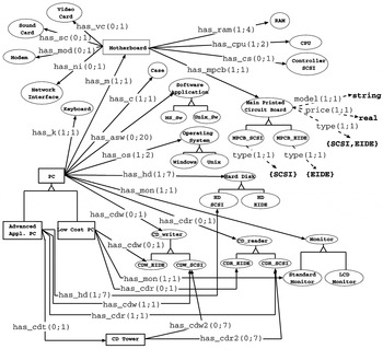
A sample (portion of a) conceptual model: the partotaxonomic knowledge.
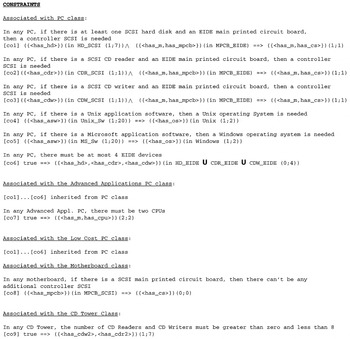
A sample (portion of a) conceptual model: the constraints.
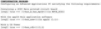
The user's requirements for an advanced application PC.

Decomposition policies
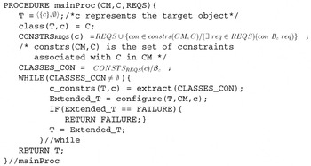
A configuration algorithm: mainProc procedure.
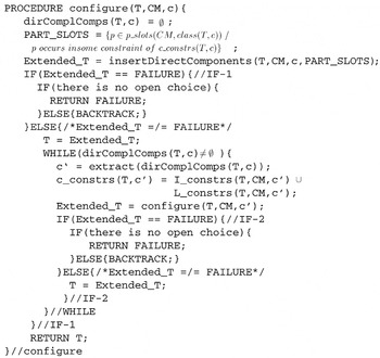
A configuration algorithm: configure procedure.
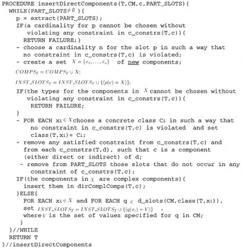
A configuration algorithm: insertDirectComponents procedure.
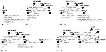
A configuration example: the first subproblem.
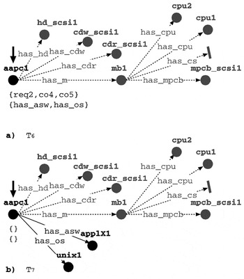
A configuration example: the second subproblem.
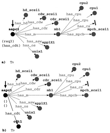
A configuration example: the third problem.
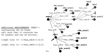
A configuration example: configuring the CD tower component.
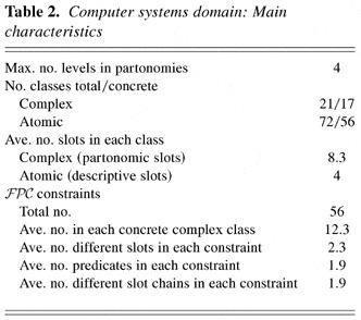
Computer systems domain: Main characteristics
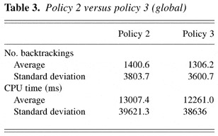
Policy 2 versus policy 3 (global)
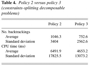
Policy 2 versus policy 3 (constraints-splitting decomposable problems)
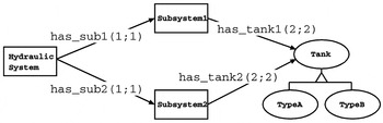
A portion of a hydraulic system conceptual model.
 You have
Access
- 13
- Cited by