INTRODUCTION
The present paper studies methods for statistical analysis of randomized complete block (RCB) experiments. In such experiments, rv experimental units are divided into r blocks, and v experimental treatments are randomly allocated to experimental units within each block, so that each of the v treatments occurs once in each block. The present study is restricted to this equireplicated design, and generalizations to unequally replicated designs are commented on in the Discussion. The standard linear statistical model for the RCB design includes two factors, block and treatment, and an error term that is assumed to be normally distributed. Often the RCB experiment is comparative, in which case the interest is in treatment contrasts (Bailey Reference Bailey2008), usually pairwise differences in treatment effects. The factor treatment can be modelled as fixed or random. When modelled as fixed, parameters are estimated for each treatment effect, whereas when modelled as random, treatment effects are predicted, assuming they belong to a parametric distribution, usually the normal. In this case, the model has two variance components: the treatment effects variance, σ G2, and the error variance, σ E2.
In the fixed effects model (i.e. when treatment is modelled as fixed), the observed differences between treatment means are the best linear unbiased estimates (BLUE) of the expected differences (e.g. Searle Reference Searle1971). In other words, the observed difference m 1−m 2 between Treatments 1 and 2 is an unbiased estimator of the expected difference between the effects of Treatments 1 and 2, and among all conceivable unbiased estimators that are linear functions of the observations, the difference m 1−m 2 is the one with the smallest variance. However, estimators that give smaller expected mean square error exist. The expected mean square error is the sum of the variance and the squared bias. Thus, if biased estimators are accepted, it is possible to use one that on average gives smaller squared errors than m 1−m 2 does. This can be accomplished, e.g. by modelling treatment as a random factor. Predictions of treatment effects, obtained through such modelling, are known as best linear unbiased predictions (BLUP). In this acronym, the letter U refers to ‘unbiased’, which in BLUP means that randomly chosen predictions of effects are zero on average. This does not imply that the difference between the predictions of Treatments 1 and 2 is an unbiased estimate of the difference between the effects of those treatments. On the contrary, the difference between the BLUPs of Treatments 1 and 2 is biased as an estimator of the true difference between the treatments.
BLUP theoretically gives smaller mean square error than fixed-effects model-based BLUE when the ratio σ G2/σ E2 is known (e.g. Robinson Reference Robinson1991). In practice, variance components must be estimated and this ratio is not known. BLUP is a shrinkage method (Copas Reference Copas1983; Gruber Reference Gruber1998); using BLUP, the prediction of a difference is closer to zero than the observed difference between the means. The prediction is shrunk towards zero through multiplication with a shrinkage multiplier, k, which is a function of σ G2/σ E2. When estimates are used, instead of actual variances, the method is called empirical best linear unbiased prediction (EBLUP). Prediction using EBLUP is adequate if the variance components are well estimated. In small experiments, this requirement is not fulfilled.
Generally, a shrinkage estimator has the form kz+(1−k)c, where z is an observation and k is a shrinkage multiplier, which is a function that takes values between 0 and 1. In other words, the shrinkage estimator is a weighted average of the observation, z, and some other estimate, c. Thus, the shrinkage estimator is shrunk towards c, which is an initial guess or an estimate based on other information. In the context of the present paper, z is an observed treatment mean, m j, whereas c is the overall mean, which will be denoted by m (i.e. the mean of treatment means). The shrinkage estimator of the jth treatment mean is m+k(m j−m). When treatment means are close to the overall mean, treatment means support the idea that all expected means can be identical. When this happens, the shrinkage multiplier, k, is small, so that shrinkage towards the overall mean is large. On the other hand, when treatment means differ much, the overall mean is most likely a poor estimate of treatment means. In this case, the shrinkage multiplier is close to 1, and shrinkage is slight. The shrinkage estimators k(m 1−m) and k(m 1−m 2), of the observed effect of Treatment 1 (i.e. m 1−m) and the observed difference between Treatments 1 and 2 (i.e. m 1−m 2), respectively, are shrunk towards c=0.
James & Stein (Reference James, Stein and Neyman1961) proposed an explicit shrinkage estimator that gives smaller root-mean-square error (RMSE) than the usual mean in the fixed effects model with three or more treatments. Based on the assumption of random treatment effects, and motivated by breeding applications, Henderson (Reference Henderson, Hanson and Robinson1963) derived equations for BLUP in linear mixed models. In these models, BLUP is equivalent to maximum likelihood estimation as based on the joint distribution of fixed effects and normally distributed random effects (e.g. Pawitan Reference Pawitan2001). Utilizing Bayesian methodology for hierarchical models, BLUPs can also be derived as empirical Bayes estimators. This is achieved by considering the distribution of unobserved random effects as a prior distribution (e.g. Searle et al. Reference Searle, Casella and McCulloch1992).
The interest of the present authors in small RCB experiments originates from agricultural field research and analysis of crop variety trials. Finney (Reference Finney1964) pointed out that selection bias is introduced in variety trials if the highest yielding varieties are chosen on the basis of their observed means. Top yielding varieties in an experiment may have performed well partly because of random errors. If the experiment were repeated, those varieties would probably not perform as well as in the first experiment (Galwey Reference Galwey2006). EBLUP shrinks the means towards the overall mean, which may give better predictions. EBLUP is often used and recommended for breeding trials, where the number of genotypes is large and the main interest is ranking and prediction of genotype effects (e.g. Real et al. Reference Real, Gordon and Hodgson2000; Smith et al. Reference Smith, Lim and Cullis2006; Piepho et al. Reference Piepho, Möhring, Melchinger and Büchse2008), although in many careful breeding studies genotype effects are traditionally modelled as fixed (e.g. Sarker et al. Reference Sarker, Singh and Erskine2001). In the context of breeding, the treatment variance estimate can be used for calculation of heritability and expected genetic advance under selection (Galwey Reference Galwey2006; Piepho & Möhring Reference Piepho and Möhring2007). Smith et al. (Reference Smith, Cullis and Gilmour2001) argued for modelling effects of varieties as random in analyses of single variety trials and series of variety trials, since this provides ‘more reliable estimates’. Cullis et al. (Reference Cullis, Smith, Hunt and Gilmour2000) reported that EBLUP is used in crop variety evaluation programmes in Australia, and measured the efficiency of such programmes using random variety effects. Smith et al. (Reference Smith, Cullis and Thompson2005) discussed the issue of modelling varieties as fixed or random, concluding that BLUE should be used when the aim of the analysis is to determine the difference between specific pairs of varieties, whereas BLUP should be used when the aim of the analysis is selection of varieties. However, they remarked that since EBLUP must be used in place of BLUP, ‘the only question that remains’ is ‘whether the estimates of the variance parameters are sufficiently precise to ensure that the optimality of BLUP is maintained’.
The present paper investigates performance of EBLUP in small RCB experiments. In crop breeding trials, the number of treatments (i.e. genetic lines) is often very large, which makes it natural and easy to model the treatment effects with a random distribution, but in official variety evaluations, in specific crops sometimes less than ten treatments (i.e. cultivars or potential cultivars) are compared. For this reason, it is interesting to investigate how large the experiments need to be for EBLUP to perform better than BLUE.
The present study was performed using simulation and the ‘mixed’ procedure in SAS (Littell et al. Reference Littell, Milliken, Stroup, Wolfinger and Shabenberger2006). Normally distributed treatment effects were simulated, corresponding to various degrees of shrinkage, obtained through varying the σ G2/σ E2 ratio. In addition, the sensitivity to the normal assumption was examined through simulation of non-normally distributed random effects. EBLUP was compared with BLUE in terms of RMSE, in estimation and prediction of means, and coverage of 0·95 confidence, prediction and credible intervals. In calculation of prediction intervals, the methods of Satterthwaite Reference Satterthwaite1946; Giesbrecht & Burns Reference Giesbrecht and Burns1985 and of Kenward & Roger (Reference Kenward and Roger1997, Reference Kenward and Roger2009) for approximating denominator degrees of freedom and calculating standard errors were compared, as well as the so-called containment method, which is the default (SAS Institute 2008). A common problem with small experiments is that the estimate of the treatment variance can be zero, so that all predictions of treatment means equal the overall mean and hence treatments cannot be separated. When this occurs, equations for approximate prediction intervals break down. Therefore, a Bayesian approach was also investigated in the present study, which, based on an assigned prior distribution of the parameters, simulates a posterior distribution of the parameters. Bayesian credible intervals for predictions were computed from random samples from posterior distributions of treatment effects, thereby avoiding the use of single-point estimates in interval calculations.
Besag & Higdon (Reference Besag and Higdon1999) analysed an RCB variety trial using Bayesian methods. Cotes et al. (Reference Cotes, Crossa, Sanches and Cornelius2006), Theobald et al. (Reference Theobald, Roberts, Talbot and Spink2006) and Ghavi Hossein-Zadeh & Ardalan (Reference Ghavi Hossein-Zadeh and Ardalan2011) have provided other examples of the usefulness of Bayesian methods in agricultural research. Several simulation studies have compared the methods of Satterthwaite (Reference Satterthwaite1946) and of Kenward & Roger (Reference Kenward and Roger1997, Reference Kenward and Roger2009) in models with fixed treatment effects and with unbalanced data structures and various covariance structures (Schaalje et al. Reference Schaalje, McBride and Fellingham2002; Chen & Wei Reference Chen and Wei2003; Guiard et al. Reference Guiard, Spilke and Dänicke2003; Savin et al. Reference Savin, Wimmer and Witkovsky2003; Spilke et al. Reference Spilke, Piepho and Meyer2004, Reference Spilke, Piepho and Hu2005). The small-sample behaviour of EBLUP v. BLUE, using the methods of Satterthwaite (Reference Satterthwaite1946) and of Kenward & Roger (Reference Kenward and Roger1997, Reference Kenward and Roger2009), has been less studied, and comparisons of BLUE and EBLUP with Bayesian approaches in the context of agricultural field experiments are rare (Theobald et al. Reference Theobald, Talbot and Nabugoomu2002; Edwards & Jannink Reference Edwards and Jannink2006). To the best of the present authors’ knowledge, these methods have not been simultaneously compared in small experimental designs such as the RCB design.
THEORY AND METHODS
Consider an RCB experiment with r replicates and v treatments. Let y ij denote the observation of the jth treatment in the ith block, i=1, 2, …, r and j=1, 2, …, v. Let
 $$y_{ij} = b_i + t_j + e_{ij} $$
where β i is a fixed effect of the ith block, τ j is a fixed effect of the jth treatment, and e ij is a normally distributed random error term. Let m j be the mean of the observations from the jth treatment, i.e. m j=Σiyij/r. The BLUE of the difference between Treatments 1 and 2 is m 1−m 2.
The present paper studies the use of the RCB model with random treatments. Let
 $$y_{ij} = b_i + u_j + e_{ij} $$
where β i is a fixed effect of the ith block, whereas u j and e ij are independent normally distributed random terms with expected value zero and variances σ G2 and σ E2, respectively. In comparative experiments, the differences between the treatments are examined, so the present study focused on the difference between two arbitrarily selected random Treatments 1 and 2.
Conditionally on u 1 and u 2 in the mixed model in Eqn (2), the bias in m 1−m 2 as a predictor of u 1−u 2 is E((m 1−m 2)−(u 1−u 2)|u 1, u 2)=0 and the variance is var(m 1−m 2|u 1, u 2)=2σ E2/r. When u 1 and u 2 vary randomly, the square root of the expected mean square error (RMSE) in m 1−m 2 is
 $${\rm RMSE}({\rm BLUE}) = \sqrt {\displaystyle{{2\sigma _{\rm E}^2} \over r}} $$
Let m=Σijyij/(rt) denote the overall mean. The best linear unbiased predictor of u j is  $\tilde u_j = k(m_j - m)$, with the shrinkage multiplier k defined as
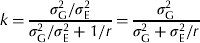 $$k = \displaystyle{{\sigma _{\rm G}^2 /\sigma _{\rm E}^2} \over {\sigma _{\rm G}^2 /\sigma _{\rm E}^2 + 1/r}} = \displaystyle{{\sigma _{\rm G}^2} \over {\sigma _{\rm G}^2 + \sigma _{\rm E}^2 /r}}$$
Conditioned on u 1 and u 2, the bias in  $\tilde u_1 - \tilde u_2 $ is E(($\tilde u_1 - \tilde u_2 $)−(u 1−u 2)| u 1, u 2)=(k−1)(u 1−u 2) and var($\tilde u_1 - \tilde u_2 $| u 1, u 2)=2k 2σ E2/r. When u 1 and u 2 vary randomly, the square root of the expected mean square error in the best linear unbiased predictor $\tilde u_1 - \tilde u_2 $ of u 1−u 2 is
 $${\rm RMSE}\left( {{\rm BLUP}} \right) = \sqrt {2(k - 1)^2 \sigma _{\rm G}^2 + \displaystyle{{2k^2 \sigma _{\rm E}^2} \over r}} = \sqrt {\displaystyle{{2k\sigma _{\rm E}^2} \over r}} $$
Let  $\hat k$ denote the empirical shrinkage multiplier, calculated as in Eqn (3), but with the restricted maximum likelihood (REML) estimates
 $\hat \sigma _{\rm G}^2 $ and
 $\hat \sigma _{\rm E}^2 $ substituted for σ G2 and σ E2, respectively, and let
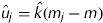 $\hat u_j = \hat k(m_j - m)$. Using the REML estimates, the empirical best linear unbiased predictor of the difference between Treatments 1 and 2 is
 $\hat u_1 - \hat u_2 = \hat k{\rm (}m_1 - m_2 {\rm )}$. The square root of the expected mean square error in this predictor of the difference between the two randomly selected Treatments 1 and 2 was investigated by simulation.
RCB experiments with r=2, 4, 6 and 8 blocks and with v=3, 6, 9 and 12 treatments were simulated using the SAS System. The observation y ij, from the ith block, i=1, 2,…, r, and the jth treatment, j=1, 2,…, v, was generated as
 $$y_{ij} = 100 + u_j + e_{ij} $$
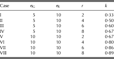
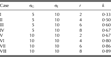
where u j and e ij were independent random numbers from distributions N(0,σ G2) and N(0,σ E2), respectively. Eight cases, denoted I–VIII, were investigated, with different values of σ G2, σ E2 and r, as specified in Table 1. These cases represent shrinkage multipliers ranging from 0·33 (Case I) to 0·89 (Case VIII). Thus, for each case of Table 1, four different experimental designs were simulated, and the complete study comprised 8×4=32 different experimental conditions (i.e. combinations of σ G2, σ E2, r and v). Each experimental condition was simulated 10000 times according to Eqn (4). Altogether 320000 normally distributed datasets were generated.
Cases investigated in simulation. Standard deviation between treatments (σG), error standard deviation (σE), number of replicates (r), and shrinkage multiplier (k)
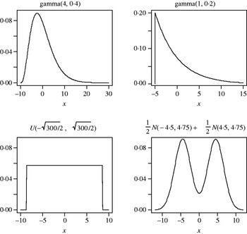
The performance of EBLUP might be sensitive to the requirement that the random effects are normally distributed. To investigate this sensitivity, observations with non-normally distributed random effects were simulated. Four non-normal distributions were investigated: (i) an exponential distribution (highly skewed), (ii) a gamma distribution (slightly skewed), (iii) a continuous uniform distribution (not skewed) and (iv) a mixture of two normal distributions (bimodal). Figure 1 shows the investigated distributions. The probability density function of gamma(α, λ) is
 $$f\,(x) = \displaystyle{1 \over {\Gamma (\alpha )}}\lambda ^\alpha x^{\alpha - 1} \,{\rm e}^{ - \lambda x}, \quad x \gt {\rm} 0$$
where α is the shape parameter and λ−1 the scale parameter. Two gamma distributions were used: gamma(1, 0·2), which is an exponential distribution with rate parameter λ=0·2, and gamma (4, 0·4). The random effects were centred around their expected values, i.e. we let u j=X−α/λ in Eqn (4), where the X is gamma(α, λ), so that E(u j)=0. The variance of a gamma(α, λ) distribution is α/λ2, which equals 25 for both distributions, so that the standard deviation is σ G=5. The chosen uniform distribution, U(−3001/2/2, 3001/2/2), has expected value 0 and variance 25. The normal mixture had mixture weights 1/2 and components N(−4·5, 4·75) and N(4·5, 4·75). This mixture also has expected value 0 and variance 25. When the random effects belong to a bimodal mixture of normal distributions, the predictions of the random effects can be unimodal (Verbeke & Lesaffre Reference Verbeke and Lesaffre1996). In practice, the mixture distribution can occur if the treatments belong to two subpopulations.
Distributions used for simulation of random effects in the study of robustness. The distributions are centred around zero and have variance 25.

The robustness was investigated for Case II (Table 1) only. Observations were generated using non-normally distributed random effects and normally distributed error effects: e ij∼N(0, σ E2), σ E=10. Again, experiments with v=3, 6, 9 and 12 treatments were simulated. Altogether 16 experimental conditions were simulated 10000 times so that 160000 non-normally distributed datasets were generated.
To each simulated dataset of rv observations, the RCB mixed model of Eqn (2) was fitted using the mixed procedure in SAS 9.2 (Littell et al. Reference Littell, Milliken, Stroup, Wolfinger and Shabenberger2006). An exemplifying SAS program can be downloaded from the Journal of Agricultural Science, Cambridge webpage (Supplementary Materials 1 and 3; available at http://journals.cambridge.org/AGS). The variance components were estimated using the REML method, constrained to give non-negative estimates. Let u jp denote the random effect u j, for the jth treatment, generated in the pth simulation of a specific experimental condition, and let  $\hat u_{\,jp} $ denote the BLUP
 $\hat u_j $ of u j in the pth simulation, P=1, 2, …, 10000. The square root of the expected mean square error in the EBLUP of the difference between Treatments 1 and 2 was estimated by
 $$\scale90%{\rm RMSE}\left( {{\rm EBLUP}} \right) = \sqrt {\displaystyle{{\sum\nolimits_{\,p = 1}^{10\,000} {((\hat u_{1p} - \hat u_{2p} ) - (u_{1p} - u_{2p} ))^2}} \over {10\,000}}} $$
For each model fit, that is for each simulated dataset and estimation method, three approximate 0·95 prediction intervals for u 1−u 2 were calculated. The calculations were performed using the containment, Satterthwaite (Reference Satterthwaite1946) and Kenward & Roger (Reference Kenward and Roger1997, Reference Kenward and Roger2009) methods, within the mixed procedure of the SAS System. Through the containment method, which is the default method of the mixed procedure, the 0·95 prediction interval is calculated as
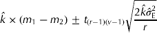 $$\hat k \times (m_1 - m_2 ) \pm t_{(r - 1)(v - 1)} \sqrt {\displaystyle{{2\hat k\hat \sigma _{\rm E}^2} \over r}} $$
where t (r −1)(v −1) denotes the 97·5th percentile of a t-distribution with (r−1)(v−1) degrees of freedom. Through the Satterthwaite (Reference Satterthwaite1946) method, the mean square error in Eqn (5) is assumed to be approximately chi-square distributed with max{1, d} degrees of freedom, where
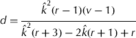 $$d = \displaystyle{{\vskip-3pt\hat k^2 (r - 1)(v - 1)} \over {\hat k^2 (r + 3) - 2\hat k(r + 1) + r}}$$
Equation (6) is derived in Appendix 1. The 0·95 prediction interval for u 1−u 2 is calculated as
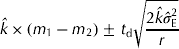 $$\hat k \times (m_1 - m_2 ) \pm t_{\rm d} \sqrt {\displaystyle{{2\hat k\hat \sigma _{\rm E}^2} \over r}} $$
where t d is the 97·5th percentile of a t-distribution with d, from Eqn (6), degrees of freedom. Prasad & Rao (Reference Prasad and Rao1990) and Kenward & Roger (Reference Kenward and Roger1997, Reference Kenward and Roger2009) considered the extent to which the estimate of the mean square error tends to be underestimated when the variance in the estimates of the variance components is not taken into account and proposed correction terms based on linear approximations. For the considered experimental design, the Kenward & Roger (Reference Kenward and Roger1997, Reference Kenward and Roger2009) 0·95 prediction interval, as implemented in the mixed procedure of the SAS System, is
 $$\hat k \times (m_1 - m_2 ) \pm t_{\rm d} \sqrt {\displaystyle{{2\hat k\hat \sigma _{\rm E}^2} \over r} + \displaystyle{{8\hat \sigma _{\rm E}^2 (1 - \hat k)} \over {(r - 1)(v - 1)}}} $$
with t d defined as in Eqn (7). The correction term  $8\hat \sigma _{\rm E}^2 (1 - \hat k)/((r - 1)(v - 1))$ in Eqn (8) is derived in Appendix 2.
When  $\hat \sigma _G^2 = 0$, also
 $\hat k = 0$ and the EBLUP
 $\hat u_1 - \hat u_2 = \hat k \times {\rm (}m_1 - m_2 {\rm )} = 0$. As a result, the approximate prediction intervals of Eqns (5), (7) and (8) break down, and the confidence in the prediction
 $\hat u_1 - \hat u_2 = 0$ cannot be expressed. In balanced experiments, the REML estimates of the variance components are the same as the ANOVA estimates, provided the latter are non-negative, and the probability of a zero REML estimate is therefore easily calculated as Pr($\hat \sigma _{\rm G}^2 = 0$)=Pr(F<(σ E2/(rσ G2+σ E2)), where F is F distributed with v−1 and (v−1)(r−1) degrees of freedom (Searle et al. Reference Searle, Casella and McCulloch1992). This probability was calculated for the examined cases and numbers of treatments.
In addition, sampling-based Bayesian analyses were performed, also using the mixed procedure. In Bayesian analysis, the prior distribution of the parameters is combined with the observed data to yield the so-called posterior distribution of the parameters, including the variance components. The method implemented in the mixed procedure uses a flat (equal to 1) prior for the fixed block effects and Jeffrey's prior (equal to the square root of the determinant of the inverse of Matrix A, in Appendix 1, Eqn (A1)) for the variance components. As the posterior distribution cannot be computed in analytical form, the mixed procedure uses an independence chain algorithm (Tierney Reference Tierney1994) to obtain samples from the posterior distribution. With a sufficiently large Monte Carlo sample, all properties of the posterior distribution (means, modes, credible intervals) can be computed with good precision. The default settings were used, but with 50000 posterior samples (the default is 1000). For each posterior sample, the mixed procedure generated random treatment effects (u 1*, u 2*) from the conditional posterior distribution of (u 1, u 2), given the parameters. The mean of u 1*−u 2* was considered as a prediction of the true difference u 1−u 2, and a 0·95 credible interval was calculated with limits set to the 2·5th and 97·5th percentiles of u 1*−u 2*.
Coverage of prediction intervals, Eqns (5), (7) and (8), and Bayesian credible intervals (i.e. frequencies of intervals covering true differences u 1−u 2), was computed. In the calculations of coverage for prediction intervals, simulated datasets for which $\hat \sigma _{\rm G}^2 = 0$ were excluded, because at these incidences prediction intervals could not be constructed. These interesting datasets were included, however, in the calculation of coverage of Bayesian credible intervals. Occasionally, the Bayesian posterior sampling was stopped by the mixed procedure, because the acceptance rate was too low. These datasets were excluded before calculation of coverage of credible intervals.
RESULTS
Normally distributed random effects
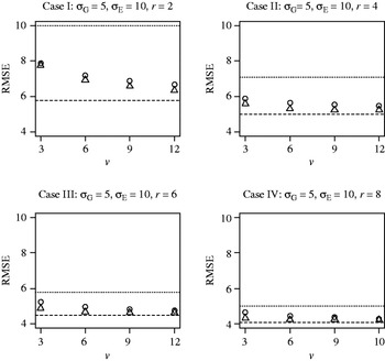
Figure 2 presents, for Cases I–IV (Table 1), simulated RMSE for EBLUP of the difference between the treatment effects. The lower dashed lines are RMSE for BLUP. These are the RMSE calculated assuming that the variances were known. When the variances were estimated (EBLUP), the observed RMSE were larger, as indicated by the circles. As a consequence of improved estimates of the variance components, larger numbers of treatments produced smaller RMSE. The upper dotted lines show the RMSE for BLUE. In Cases I–IV, EBLUP was always better than BLUE with regard to RMSE, also when the number of replicates and the number of treatments were small. The Bayesian analysis produced slightly smaller RMSE than the EBLUP, as seen by comparing triangles with circles.
RMSE in a difference between two treatments, using BLUE (dotted line), BLUP (dashed line), EBLUP (circles) and Bayesian posterior means (triangles) when the treatment standard deviation σ G is 5, the error standard deviation σ E is 10, the number of blocks is r=2, 4, 6 and 8, and the number of treatments is v=3, 6, 9 and 12.

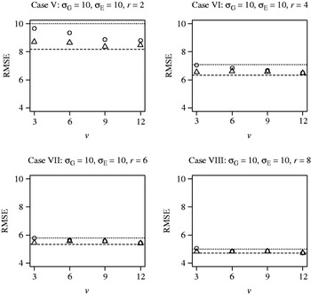
Figure 3 illustrates Cases V–VIII. In these cases the shrinkage multiplier was larger than in the corresponding Cases I–IV. Consequently, the differences between RMSE of BLUP and RMSE of BLUE were smaller. In Cases VII and VIII the RMSE of EBLUP was larger than the RMSE of BLUE, when the experiment comprised only three treatments. In these situations it was slightly better to use simple averages than to use EBLUP, because the variance components were poorly estimated. In Case VI with three treatments, the difference between EBLUP and BLUE was very small. In all other simulations, EBLUP outperformed BLUE. The means of the Bayesian posterior samples (triangles) showed smaller RMSE than EBLUP (circles).
RMSE in a difference between two treatments, using BLUE (dotted line), BLUP (dashed line), EBLUP (circles) and Bayesian posterior means (triangles) when the treatment standard deviation σ G is 10, the error standard deviation σ E is 10, the number of blocks is r=2, 4, 6 and 8, and the number of treatments is v=3, 6, 9 and 12.

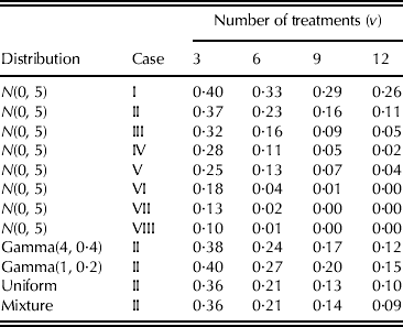
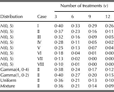
The first eight rows of Table 2 show computed theoretical probabilities of the treatment variance σ G2 being estimated to be zero. The observed frequencies of zero estimates were close to the theoretical probabilities. When the shrinkage multiplier (cf. Table 1) and the numbers of treatments are small, the probability of the variance between treatments being estimated to be zero is not negligible. At these occurrences, Eqns (5), (7) and (8) cannot measure the precision in the predictions. For 0·0015 of the datasets, the Bayesian posterior sampling was stopped by the mixed procedure, because of a low acceptance rate.
Probabilities of the estimator $\hat \sigma _{\rm G}^2 $ being zero (exact probabilities for the normal distribution and observed frequencies for the non-normal distributions)
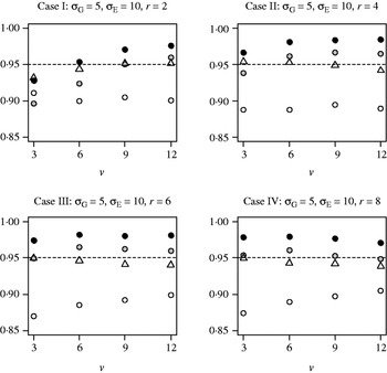
Figures 4 and 5 report coverage of prediction intervals and credible intervals. Figure 4 shows the results for Cases I–IV. Without any adjustment of degrees of freedom (unfilled circles), coverage of the approximate 0·95 prediction intervals was too small. Using the Satterthwaite (Reference Satterthwaite1946) method (shaded circles), coverage was usually much improved. The Kenward & Roger (Reference Kenward and Roger1997, Reference Kenward and Roger2009) method (filled circles) often produced prediction intervals that were too wide. In most situations, the Bayesian credible intervals showed coverage close to the nominal level 0·95.
Coverage of 0·95 prediction intervals for a difference between two treatments using the containment method (unfilled circles), the Satterthwaite (Reference Satterthwaite1946) method (shaded circles) and the Kenward & Roger (Reference Kenward and Roger1997, Reference Kenward and Roger2009) method (filled circles), and coverage of 0·95 credible intervals for a difference between two treatments using the Bayesian method (triangles), when the treatment standard deviation σ G is 5, the error standard deviation σ E is 10, the number of blocks is r=2, 4, 6 and 8, and the number of treatments is v=3, 6, 9 and 12. The dashed line indicates the nominal level 0·95.

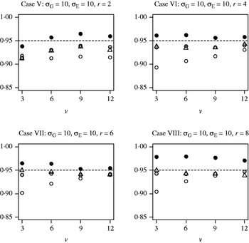
Coverage of 0·95 prediction intervals for a difference between two treatments using the containment method (unfilled circles), the Satterthwaite (Reference Satterthwaite1946) method (shaded circles) and the Kenward & Roger (Reference Kenward and Roger1997, Reference Kenward and Roger2009) method (filled circles), and coverage of 0·95 credible intervals for a difference between two treatments using the Bayesian method (triangles), when the treatment standard deviation σ G is 10, the error standard deviation σ E is 10, the number of blocks is r=2, 4, 6 and 8, and the number of treatments is v=3, 6, 9 and 12. The dashed line indicates the nominal level 0·95.

Also in Cases V–VIII (Fig. 5), the containment method (unfilled circles) produced prediction intervals that were too small. The Satterthwaite (Reference Satterthwaite1946) approximation (shaded circles) improved coverage. The Kenward & Roger (Reference Kenward and Roger1997, Reference Kenward and Roger2009) method (filled circles) tended to produce prediction intervals that were slightly too wide. The Bayesian (triangles) and the Satterthwaite (Reference Satterthwaite1946); shaded circles) methods gave similar coverage.
The comparisons in Figs 4 and 5, between EBLUP and the Bayesian method is of practical value, but they are not strictly fair, because the calculations of coverage were made on partly different datasets: simulated datasets for which $\hat \sigma _{\rm G}^2 = 0$ were excluded from the calculations of coverage of prediction intervals, since no such calculations could be made, and simulated datasets for which the Bayesian posterior sampling failed were excluded from the calculation of coverage of the Bayesian credible intervals. This reflects what would be done in practice: when a method fails, the results are discarded, and another method is used. However, a fair comparison of the methods was also conducted, using all simulated datasets with both positive $\hat \sigma _{\rm G}^2 $ and successful Bayesian sampling. The results obtained were similar to those in Figs 4 and 5 (not shown), but in Case I with three and six treatments and Case II with three treatments the Bayesian method gave similar coverage as the Satterthwaite (Reference Satterthwaite1946) method, and in Case V with three treatments, coverage of the Bayesian method was 0·90.
Study of robustness: non-normally distributed random effects
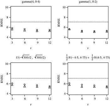
Figure 6 compares EBLUP (circles) and the Bayesian method (triangles) with each other and with BLUE (dotted line) for the four non-normal distributions included in the study. The normal-theory based EBLUP performed appreciably better than BLUE with regard to RMSE. The difference between EBLUP and the Bayesian approach was small, but Bayesian posterior means produced slightly smaller RMSE than EBLUP.
RMSE in a difference between two treatments, using BLUE (dotted line), EBLUP (circles) and Bayesian posterior means (triangles) when the treatment standard deviation σ G is 5, the error standard deviation σ E is 10, for four different non-normal treatment distributions (cf. Fig. 1), and with number of treatments v=3, 6, 9 and 12.

The last four rows of Table 2 reports the observed frequencies of the treatment variance σ G2 being estimated to be zero. Gamma distributed random effects resulted in zero estimates more often than normally distributed random effects (Case II), but uniform and mixture distributed random effects gave zero estimates less often. The Bayesian posterior sampling failed in 0·0023 of all non-normally distributed datasets.
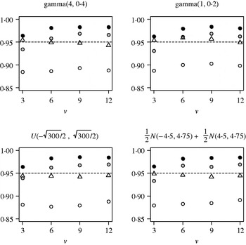
Figure 7 illustrates observed coverage of 0·95 prediction intervals and 0·95 credible intervals for the non-normal distributions. The containment method gave much too low coverage, often smaller than 0·90, and the Kenward & Roger (Reference Kenward and Roger1997, Reference Kenward and Roger2009) method produced too large coverage. In most situations, the Satterthwaite (Reference Satterthwaite1946) method resulted in coverage closer to the nominal level 0·95 than the Kenward & Roger (Reference Kenward and Roger1997, Reference Kenward and Roger2009) method. The Bayesian method outperformed the other methods, usually presenting coverage very close to 0·95.
Coverage of 0·95 prediction intervals for a difference between two treatments using the containment method (unfilled circles), the Satterthwaite (Reference Satterthwaite1946) method (shaded circles) and the Kenward & Roger (Reference Kenward and Roger1997, Reference Kenward and Roger2009) method (filled circles), and coverage of 0·95 credible intervals for a difference between two treatments using the Bayesian method (triangles), when the treatment standard deviation σ G is 5, the error standard deviation σ E is 10, for four different non-normal treatment distributions (cf. Fig. 1), and with number of treatments v=3, 6, 9 and 12. The dashed line indicates the nominal level 0·95.

A counterpart to Fig. 7, based on all simulated datasets with both positive $\hat \sigma _{\rm G}^2 $ and successful Bayesian sampling, looked almost identical to Fig. 7. However, in this figure, coverage of the Bayesian credible intervals was approx. 0·94 in experiments with three treatments, regardless of the probability distribution (not shown).
DISCUSSION
The present paper studied comparative RCB experiments with small numbers of treatments. The RCB design is appropriate when the number of treatments is small; otherwise resolvable incomplete block designs are recommended (John & Williams Reference John and Williams1995), for example alpha designs (Patterson & Williams Reference Patterson and Williams1976). For a comparison of BLUP and BLUE for incomplete block designs, see Piepho & Williams (Reference Piepho and Williams2006). A comparison of Bayesian methods with BLUP for this kind of design would be interesting, but is beyond the scope of the present paper.
Arguments against using EBLUP in small RCB experiments include:
1. The treatment effects cannot reasonably be regarded as randomly sampled from a normal distribution.
2. In small experiments, the variance components may be imprecisely estimated, with poor predictions of the random effects as a result.
3. There are no exact methods for statistical inference on random effects.
Regarding Argument 1, the present study indicated that EBLUP performs well in small RCB experiments also if the distribution of the random effects is not normal: the RMSE of EBLUP was consistently smaller than with BLUE in the simulated experiments with non-normally distributed random effects. This result is not surprising considering the theoretical result derived by James & Stein (Reference James, Stein and Neyman1961) that shrunken means can give smaller RMSE than simple means in a model with fixed treatment effects. In the fixed-effects model, the gain of shrinkage of treatment means towards the overall mean is largest when all (unobservable) expected means are the same. In this case, observed treatment means differ only because of random errors, and the overall mean is the common best estimator. When the expected means differ, as they usually do, the potential gain in RMSE of shrinkage towards the overall mean still exists, although it is smaller. As mentioned in the Introduction, when observed means are similar, this supports the overall mean as an initial estimate of expected treatment means, which makes shrinkage estimation efficient. It should be noticed that for this result, treatment effects need not be random. Lee et al. (Reference Lee, Nelder and Pawitan2006) pointed out the similarity between the James-Stein estimator and BLUP in the one-way model for completely randomized experiments.
In practice, when there are few treatments, it is difficult to determine whether the treatments can be regarded as sampled from a normal distribution or not. Sometimes the treatments of the experiment, for example the varieties in a crop variety trial, can be considered as a subset of a larger set of treatments with approximately normally distributed effects. However, Stanek (Reference Stanek, Gregoire, Brillinger, Diggle, Russek-Cohen, Warren and Wolfinger1997) proved that BLUP can be better than BLUE in sampling from finite populations of random effects, and argued that the effects can be modelled as random although the population of random effects is not larger than the sample. In this view, the treatments of the experiment need not be a sample from a larger population of treatments in order to justify the use of BLUP.
The results of the present simulation study indicated that imprecise estimates of variance components (Argument 2, above) are not a severe problem for the use of EBLUP in small RCB experiments. Usually the RMSE of EBLUP was smaller, or only slightly larger, than the RMSE of BLUE, even when the number of treatments was small. The simulations showed that the methods of Satterthwaite (Reference Satterthwaite1946) and Kenward & Roger (Reference Kenward and Roger1997, Reference Kenward and Roger2009), and also the Bayesian method, performed well in most situations, which mitigates Argument 3 to a large extent.
In RCB experiments, with one observation per treatment in each block, the ranking of treatments is the same whether BLUE or EBLUP is used, but when replication is unequal, the two methods may rank the treatments differently (e.g. Galwey Reference Galwey2006). The simulation study of the present paper was restricted to the standard, balanced, RCB experiment as defined in the Introduction. In practice, unequal replication often occurs, for example when some observations are missing or when some treatments have extra replication. When extended to unequal replication, there are many variations of the RCB experiment, some of which are orthogonal (John & Williams Reference John and Williams1995). It would be interesting to investigate the performance of BLUP and Bayesian prediction under various unbalanced scenarios with missing data or extra replication. A simulation study of such small block experiments was beyond the scope of the present paper. Piepho & Williams (Reference Piepho and Williams2006) showed that EBLUP outperformed BLUE in large (120 treatments) incomplete block experiments.
When the treatment-effects variance is estimated to be zero, which frequently happens when the number of treatments is small, prediction intervals cannot be constructed for EBLUP, so the present method is practically useless in this case. The Bayesian method does not share this problem. Moreover, the Bayesian method usually performed better than the other methods with regard to RMSE and coverage. Thus, the Bayesian framework is particularly appealing, even for researchers more inclined towards frequentist methods of analysis. The present results may be of special interest to users of the open source software R (www.r-project.org, verified 6 April 2012). The lmer function, in the R package lme4, for fitting mixed models does not include the methods of Satterthwaite (Reference Satterthwaite1946) or Kenward & Roger (Reference Kenward and Roger1997, Reference Kenward and Roger2009). An R script for analysis of an RCB experiment with fixed block effects and random treatment effects, including computation of prediction intervals based on the approximations of Satterthwaite (Reference Satterthwaite1946) and Kenward & Roger (Reference Kenward and Roger1997, Reference Kenward and Roger2009), can be downloaded from the Journal of Agricultural Science website (Supplementary Material 2 & 3; go to http://journals.cambridge.org/AGS). In a discussion about the absence of P values in R when using the lmer function, Bates (Reference Bates2006) advocated the use of Markov chain Monte Carlo methods in place of methods for approximating degrees of freedoms. Bayesian posterior sampling can be performed using the R function mcmcsamp, but this function does not reproduce the mixed procedure in SAS. The performance of the mcmcsamp function was not investigated and coverage intervals in R will probably differ from those obtained using the mixed procedure. In SAS, other Bayesian analyses can be performed using the mcmc procedure. Albert (Reference Albert2009) provided many examples of how to perform Bayesian modelling in R.
In Bayesian analysis, conventional probability values cannot be computed. However, the probability that one treatment is better than another, which is not meaningful using standard frequentist methods (Cohen Reference Cohen1994), can be calculated from the Bayesian posterior distribution. Generally confidence, prediction or credible intervals are preferred to P values, since the latter do not express precision of estimates and do not represent the kind of probability that many practitioners would be most interested in.
Jeffrey's prior was used in the simulations. This prior is vague (intended for situations where no information is available about the variance components) and improper (it does not integrate to 1). For RCB experiments with fixed block effects and random treatment effects, Jeffrey's prior gives proper posterior distributions when the number of treatments, v, is larger than the number of replicates, r (Datta & Smith Reference Datta and Smith2003, Theorem 1). Notably, the method performed well with regard to RMSE and coverage even when this condition was not fulfilled. In applications, proper prior distributions, for example inverse gamma distributions might be preferred, especially since this makes it possible to include prior information in the analyses, which should increase the benefit from the Bayesian approach.
In the present paper, the Bayesian method studied used vague improper prior distributions and an independence chain algorithm for posterior sampling. Minimum mean square error in treatment differences, and coverage of 0·95 confidence, prediction and credible intervals for treatment differences, were used as criteria for assessment of method performance. Prediction intervals were constructed using the methods of Satterthwaite (Reference Satterthwaite1946) and Kenward & Roger (Reference Kenward and Roger1997, Reference Kenward and Roger2009), as implemented in the mixed procedure of SAS. Based on the results of the present paper, the following conclusions can be made regarding modelling of small RCB experiments with normally distributed errors: (i) When the treatment effects are normally distributed, a model with normally distributed random effects can be recommended, even if the number of treatments is small; (ii) Also if the random effects are not normally distributed, the model with normally distributed random effects is often preferable to the model with fixed treatment effects; (iii) The sampling-based Bayesian method can be recommended for inference about differences in random treatment effects; and (iv) EBLUP and the use of Bayesian inference deserve further study in other settings, especially in experiments where degrees of freedom approximations may not be satisfactory, for example in block experiments with extra replication in some treatments or with missing data.
SUPPLEMENTARY MATERIAL REFERENCES
Supplementary Material 1. FORKMAN, J. & PIEPHO, H-P. Online supplementary material 1 SAS example.sas Journal of Agricultural Science, Cambridge Year; Suppl. Mat1 (http://journals.cambridge.org/AGS).
Supplementary Material 2. FORKMAN, J. & PIEPHO, H-P. Online supplementary material 2 R example.sas Journal of Agricultural Science, Cambridge Year; Suppl. Mat2 (http://journals.cambridge.org/AGS).
Supplementary Material 3. FORKMAN, J. & PIEPHO, H-P. Online supplementary material 3 Comments to examples.docx Journal of Agricultural Science, Cambridge Year; Suppl. Mat3 (http://journals.cambridge.org/AGS).
We thank the editors and the anonymous reviewers for suggestions that improved the manuscript. H. P. Piepho was supported by the GABI GAIN project (grant no FKZ0315072C).
APPENDIX 1
For the problem of approximating a linear combination of mean squares with a chi-square distribution, Satterthwaite (Reference Satterthwaite1946) utilized the result that a chi-square distributed random variable Y has 2(E(Y))2/var(Y) degrees of freedom. The Satterthwaite method for mixed models (Giesbrecht & Burns Reference Giesbrecht and Burns1985) is a generalization of the original method. Considering the standard error in Eqn (5), it is assumed that Y, defined as  $Y = 2\hat k\hat \sigma _{\rm E}^2 /r$, is approximately chi-square distributed with d=2(E(Y))2/var(Y) degrees of freedom. Provided that
 $\hat \sigma _{\rm G}^2 \gt 0$, the REML estimators $\hat \sigma _{\rm G}^2 $ and $\hat \sigma _{\rm E}^2 $ equal the ANOVA estimators with known covariance matrix (Searle Reference Searle1971).
 $$\scale90%\eqalign{{\bf A} &= {\rm var}{\rm (}\hat \sigma _{\rm G}^2, \hat \sigma _{\rm E}^2 {\rm )}' \cr&= \left( {\matrix{ {\displaystyle{2 \over {r^2}} \left( {\displaystyle{{{\rm (}r\sigma _{\rm G}^2 + \sigma _{\rm E}^2 {\rm )}^2} \over {v - 1}} + \displaystyle{{\sigma _{\rm E}^4} \over {{\rm (}r - 1{\rm )(}v - 1{\rm )}}}} \right)} & {\displaystyle{{ - 2\sigma _{\rm E}^4} \over {{\rm (}r - 1{\rm )(}v - 1{\rm )}}}} \cr {\displaystyle{{ - 2\sigma _{\rm E}^4} \over {{\rm (}r - 1{\rm )(}v - 1{\rm )}}}} & {\displaystyle{{2\sigma _{\rm E}^4} \over {r{\rm (}r - 1{\rm )(}v - 1{\rm )}}}} \cr}} \right)$$
The observed covariance matrix  ${\bf \hat A}$ is (A1), with $\hat \sigma _{\rm G}^2 $ and $\hat \sigma _{\rm E}^2 $ substituted for σ G2 and σ E2, respectively. Let
 ${\bf g}\prime = (\partial Y/\partial \hat \sigma _{\rm G}^2, \quad \partial Y/\partial \hat \sigma _{\rm E}^2 ) = (2(1 - \hat k)^2, \quad 2\hat k^2 /r)$.
Then  ${\bf g'}{\bf \hat Ag}$ approximates var(Y). The Satterthwaite approximation of the degrees of freedom is
 $2Y^2 /{\bf g'}{\bf \hat Ag}$, which can be written as Eqn (6).
APPENDIX 2
Let y be the vector of all observations y ij, sorted first by treatments and then by replicates. Model (2) can be written y=Xβ+Zu+e, where X=1v⊗Ir; β=(β 1,β 2,…,β r)'; Z=Iv⊗1r; u=(u 1,u 2,…,u v)'; e=(e 11, e 21,…,e vr)'; u is MVN(0, G); G=σ G2Iv; e is MVN(0, R); R=σ E2Irv. Then V=ZGZ'+R=It⊗ (σ G2Jr+σ E2Ir), where Jr is a matrix of ones, and V−1=It⊗(σ G2Jr+σ E2Ir)−1=It⊗((Ir−σ G2/(rσ G2+σ E2)Jr)/σ E2). For the prediction of u 1−u 2, let m denote the v-vector (1,−1, 0, …, 0)', and b'=m' GZ' V−1=(1'r(1−k) σ G2/σ E2, −1'r (1−k) σ G2/σ E2, 0, …,0). Prasad & Rao (Reference Prasad and Rao1990) proposed the correction term λ=trace(d'VdA), where d=(∂b/∂σ G2,∂b/∂σ E2) and A is defined as in Appendix 1. Since
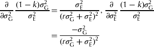 $$\displaystyle{\partial \over {\partial \sigma _{\rm G}^2}} \,\displaystyle{{(1 - k)\sigma _{\rm G}^2} \over {\sigma _{\rm E}^2}} = \displaystyle{{\sigma _{\rm E}^2} \over {(r\sigma _{\rm G}^2 + \sigma _{\rm E}^2 )^2}}, \,\displaystyle{\partial \over {\partial \sigma _{\rm E}^2}} \,\displaystyle{{(1 - k)\sigma _{\rm G}^2} \over {\sigma _{\rm E}^2}} = \displaystyle{{ - \sigma _{\rm G}^2} \over {(r\sigma _{\rm G}^2 + \sigma _{\rm E}^2 )^2}} $$
algebra gives λ=4σ E2(1−k)/((r−1)(v−1)). The Kenward and Roger method adds  $2\hat \lambda $ to the mean square error in the prediction of u 1−u 2, where
 $\hat \lambda $ equals λ, but with $\hat \sigma _{\rm G}^2 $ and $\hat \sigma _{\rm E}^2 $ substituted for σ G2 andσ E2, respectively.