1 Introduction
Gravity currents are key features that affect ocean, atmospheric and coastal circulation (Lilly Reference Lilly1983; Baringer & Price Reference Baringer and Price2001; Farmer & Armi Reference Farmer and Armi2001). In the ocean, dense currents descend the continental slope over long distances, moving onto steeper slopes before encountering the ocean bottom or interleaving at their level of neutral buoyancy. Ambient water and sediment from the bottom are entrained and mixed, thus changing the properties of water masses. This is of interest, for example, for the global thermohaline circulation (Wunsch Reference Wunsch2002).
In the atmosphere, gravity currents occur as katabatic, i.e. local downslope, winds and are dominant in mountain areas. They are decoupled from the synoptic-scale winds due to abrupt changes in topography (Fernando Reference Fernando2012). These currents bring cold air into the valleys and can cause strong inversions with poor vertical mixing which affects local air quality (see Fernando Reference Fernando1999). Some other spectacular examples of gravity currents in mountain areas are snow avalanches (Hopfinger Reference Hopfinger1983; Rastello & Hopfinger Reference Rastello and Hopfinger2004) and pyroclastic flows due to volcanic eruptions (Calder et al. Reference Calder, Cole, Dade, Druitt, Hoblitt, Huppert, Ritchie, Sparks and Young1999).
Laboratory studies of gravity currents have been essential for an understanding of their dynamics. Most of these studies have focused on gravity currents on horizontal or inclined boundaries, where the head is an essential feature of the flow (see Simpson Reference Simpson1982). Ellison & Turner (Reference Ellison and Turner1959) conducted the first experiments on a steady downslope flow and also developed the now classical similarity theory of these flows (Turner Reference Turner1973). The behaviour of the front of gravity currents on slopes has been investigated by Middleton (Reference Middleton1966), Hopfinger & Tochon-Danguy (Reference Hopfinger and Tochon-Danguy1977) and Britter & Linden (Reference Britter and Linden1980), who considered the whole slope range from
 $5^{\circ }$
up to
 $90^{\circ }$
. Beghin, Hopfinger & Britter (Reference Beghin, Hopfinger and Britter1981) studied the equivalent finite-volume-release gravitational flow, spanning the whole slope range. Experiments with finite-volume-release gravity flows on slopes have also been conducted by Luthi (Reference Luthi1990) and Maxworthy & Nokes (Reference Maxworthy and Nokes2007). Haertel, Meiburg & Necker (Reference Haertel, Meiburg and Necker2000) conducted the first numerical simulations (see also Etienne, Rastello & Hopfinger Reference Etienne, Rastello and Hopfinger2006), and Altinakar, Graf & Hopfinger (Reference Altinakar, Graf and Hopfinger1990) studied turbidity currents on nearly horizontal boundaries. Turbidity currents on slopes can also accelerate due to sediment entrainment (Parker, Fukushima & Pantin Reference Parker, Fukushima and Pantin1986; Rastello & Hopfinger Reference Rastello and Hopfinger2004).
The initial developing region of the current, before reaching constant Richardson number conditions, was investigated by Pawlak & Armi (Reference Pawlak and Armi2000), who studied experimentally the development of an accelerating current on linear inclines with slope angles ranging from approximately
 $4^{\circ }$
up to
 $15^{\circ }$
. Two dynamically distinct regions were identified: a rapidly accelerating low-interfacial-Richardson-number region (
 $J=g_{0}^{\prime }\unicode[STIX]{x1D6FF}_{I\unicode[STIX]{x1D708}}/u_{m}^{2}$
, where
 $g_{0}^{\prime }$
is the buoyant acceleration supplied at the gate,
 $\unicode[STIX]{x1D6FF}_{I\unicode[STIX]{x1D708}}$
is the velocity shear layer thickness and
 $u_{m}^{2}$
is the maximum velocity) with Kelvin–Helmholtz (KH) billows development and a subsequent higher-Richardson-number region with collapse of these billows corresponding with a nearly constant mean flow velocity, further called the equilibrium state velocity. Using this Richardson criterion, they estimated the distance required for the flow to reach these two states assuming a linear increase of the shear layer, and an internal hydraulic theory. This equilibrium state velocity is characterized by a constant or nearly constant velocity due to a balance between buoyancy and total friction, and is reached at a downstream distance of the order of
 $10h_{0}$
, where
 $h_{0}$
is the initial depth of the current.
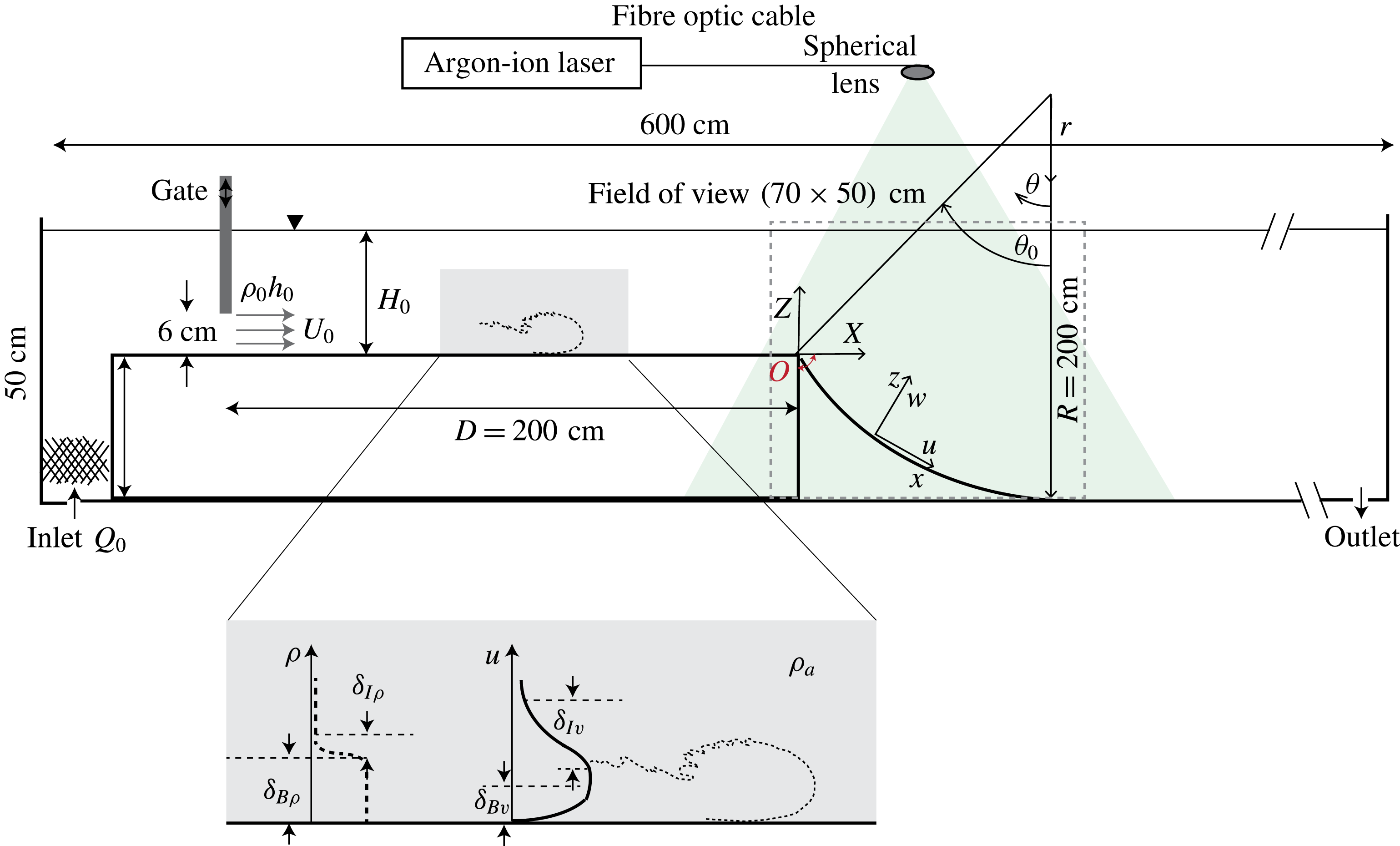
In this paper, we consider gravity currents that flow from a horizontal to a sloping boundary of constant slope angle or concave boundary, i.e. with a slope angle that decreases with downstream distance. This situation is of interest scientifically, because it is different from previously investigated flow conditions and, more importantly, because, schematically, it represents natural conditions. The difference with respect to the study of Pawlak & Armi (Reference Pawlak and Armi2000) is that here, at the start of the slope (i.e. at
 $x=0$
in figure 1), the interfacial Richardson number
 $J$
is larger than the critical value for onset of interfacial instability because the interface is relatively thick. At
 $x=0$
, the current will start to accelerate rapidly (nearly like free fall) until the Richardson number reaches a value below critical. The resulting interfacial instability causes, by means of KH billows, strong entrainment of ambient fluid, local high bottom drag and hence a rapid slowdown of the current. The question is whether the current, under these conditions, still approaches an equilibrium state in a monotonic way, as has been shown by Pawlak & Armi (Reference Pawlak and Armi2000). It should be noted that here, at
 $x=0$
, the slope angle ranges from
 $15$
to
 $31.5^{\circ }$
and thus extends the range considered by Pawlak & Armi (Reference Pawlak and Armi2000). The results show that for the present conditions, i.e. large interfacial Richardson number at
 $x=0$
, an equilibrium state is never reached over the investigated distance of
 $30h_{0}$
. Instead, the flow passes through acceleration and deceleration phases.
Sketch of the experimental set-up and definition of notations. We recall that
 $x=R(\unicode[STIX]{x1D703}_{0}-\unicode[STIX]{x1D703})$
and
 $z=(R-r)$
.

In § 2, the governing equations are derived, followed by a description of the experimental set-up and the measurement techniques in § 3. In § 4, we present experimental data characterizing the gravity current on the initial horizontal wall, giving thus the initial conditions. Experimental results over the sloping concave bottoms are presented in § 5 and a comparison with the straight slope is made in § 6. A scaling analysis that compares present with former results is discussed in § 7, and concluding remarks and future work are presented in § 8.
2 Theoretical analysis
We start from the general governing equation and then proceed with the depth-integrated equations, following closely the procedure given in Turner (Reference Turner1973). The flow is considered to be two-dimensional. Using the boundary layer and Boussinesq approximations, the momentum and continuity equations in cylindrical coordinates are
 $$\begin{eqnarray}\displaystyle & \displaystyle -\frac{\unicode[STIX]{x2202}u}{\unicode[STIX]{x2202}t}+\frac{u}{r}\frac{\unicode[STIX]{x2202}u}{\unicode[STIX]{x2202}\unicode[STIX]{x1D703}}+w\frac{\unicode[STIX]{x2202}u}{\unicode[STIX]{x2202}r}+\frac{uw}{r}=-\frac{1}{\unicode[STIX]{x1D70C}_{0}r}\frac{\unicode[STIX]{x2202}p}{\unicode[STIX]{x2202}\unicode[STIX]{x1D703}}-g\frac{\unicode[STIX]{x0394}\unicode[STIX]{x1D70C}}{\unicode[STIX]{x1D70C}_{0}}\sin \unicode[STIX]{x1D703}+\frac{\unicode[STIX]{x2202}}{\unicode[STIX]{x2202}r}\left(-\frac{\unicode[STIX]{x1D70F}}{\unicode[STIX]{x1D70C}_{0}}\right), & \displaystyle\end{eqnarray}$$
 $$\begin{eqnarray}\displaystyle & \displaystyle -\frac{\unicode[STIX]{x2202}w}{\unicode[STIX]{x2202}t}+w\frac{\unicode[STIX]{x2202}w}{\unicode[STIX]{x2202}r}+\frac{u}{r}\frac{\unicode[STIX]{x2202}w}{\unicode[STIX]{x2202}\unicode[STIX]{x1D703}}-\frac{u^{2}}{r}=-\frac{1}{\unicode[STIX]{x1D70C}_{0}}\frac{\unicode[STIX]{x2202}p}{\unicode[STIX]{x2202}r}+g\frac{\unicode[STIX]{x0394}\unicode[STIX]{x1D70C}}{\unicode[STIX]{x1D70C}_{0}}\cos \unicode[STIX]{x1D703}, & \displaystyle\end{eqnarray}$$
 $$\begin{eqnarray}\displaystyle & \displaystyle \frac{\unicode[STIX]{x2202}w}{\unicode[STIX]{x2202}r}+\frac{1}{r}\frac{\unicode[STIX]{x2202}u}{\unicode[STIX]{x2202}\unicode[STIX]{x1D703}}=0, & \displaystyle\end{eqnarray}$$
 $(u,w)$
are the velocity components opposite to the
 $\unicode[STIX]{x1D703}$
and
 $r$
directions respectively (see figure 1),
 $p$
is the pressure,
 $\unicode[STIX]{x0394}\unicode[STIX]{x1D70C}=\unicode[STIX]{x1D70C}-\unicode[STIX]{x1D70C}_{0}$
, with
 $\unicode[STIX]{x1D70C}_{0}$
the density of the ambient fluid, and
 $\unicode[STIX]{x1D70F}$
is the wall shear stress. (For geometric reasons, we preferred to define
 $\unicode[STIX]{x1D703}$
and
 $r$
in directions opposite to the flow direction (figure 1) and then change to variables
 $(x,z)$
.) Assuming a stationary flow, using the boundary layer approximation, for which
 $w\sim u(h/R)$
, with
 $h$
being the current height, and using the continuity equation, the momentum equations reduce to
 $$\begin{eqnarray}\displaystyle & \displaystyle \frac{1}{R}\frac{\unicode[STIX]{x2202}u^{2}}{\unicode[STIX]{x2202}\unicode[STIX]{x1D703}}+\frac{\unicode[STIX]{x2202}uw}{\unicode[STIX]{x2202}r}=-\frac{1}{\unicode[STIX]{x1D70C}_{0}R}\frac{\unicode[STIX]{x2202}p}{\unicode[STIX]{x2202}\unicode[STIX]{x1D703}}-g^{\prime }\sin \unicode[STIX]{x1D703}+\frac{\unicode[STIX]{x2202}}{\unicode[STIX]{x2202}r}\left(-\frac{\unicode[STIX]{x1D70F}}{\unicode[STIX]{x1D70C}_{0}}\right), & \displaystyle\end{eqnarray}$$
 $$\begin{eqnarray}\displaystyle & \displaystyle -\frac{u^{2}}{R}=-\frac{1}{\unicode[STIX]{x1D70C}_{0}}\frac{\unicode[STIX]{x2202}p}{\unicode[STIX]{x2202}r}+g^{\prime }\cos \unicode[STIX]{x1D703}, & \displaystyle\end{eqnarray}$$
 $g^{\prime }=g\unicode[STIX]{x0394}\unicode[STIX]{x1D70C}/\unicode[STIX]{x1D70C}$
and
 $r$
has been approximated by
 $r=(R-z)=R(1-z/R)\approx R$
assuming a small curvature. We now change variables to
 $x=R(\unicode[STIX]{x1D703}_{0}-\unicode[STIX]{x1D703})$
and
 $z=(R-r)$
, and integrate (2.2b
) in the
 $z$
direction to get the expression for the pressure,
 $$\begin{eqnarray}p=p_{a}+\unicode[STIX]{x1D70C}_{0}\int _{z}^{\infty }g^{\prime }\cos \unicode[STIX]{x1D703}\,\text{d}z+\unicode[STIX]{x1D70C}_{0}\int _{z}^{\infty }\frac{u^{2}}{R}\,\text{d}z.\end{eqnarray}$$
Substitution in (2.2a ) yields
 $$\begin{eqnarray}\frac{\unicode[STIX]{x2202}u^{2}}{\unicode[STIX]{x2202}x}+\frac{\unicode[STIX]{x2202}uw}{\unicode[STIX]{x2202}z}=-g^{\prime }\sin \unicode[STIX]{x1D703}-\frac{\unicode[STIX]{x2202}}{\unicode[STIX]{x2202}x}\int _{z}^{\infty }\left(g^{\prime }\cos \unicode[STIX]{x1D703}+\frac{u^{2}}{R}\right)\,\text{d}z+\frac{\unicode[STIX]{x2202}}{\unicode[STIX]{x2202}z}\left(\frac{\unicode[STIX]{x1D70F}}{\unicode[STIX]{x1D70C}_{0}}\right).\end{eqnarray}$$
To further simplify the equations, we make use of the similarity hypothesis,
 $$\begin{eqnarray}\displaystyle \displaystyle u(z,x) & = & \displaystyle U(x)f(z^{\star }),\end{eqnarray}$$
 $$\begin{eqnarray}\displaystyle \displaystyle g^{\prime }(z,x) & = & \displaystyle \overline{g}^{\prime }(x)f_{\unicode[STIX]{x1D70C}}(z^{\star }),\end{eqnarray}$$
where
 $z^{\star }=z/h$
and
 $\int _{0}^{\infty }f(z^{\star })\,\text{d}z^{\star }=1$
. The similarity assumption implies that the velocity and density profiles do not depend on
 $x$
. This is, of course, not strictly true, as indicated by the shape factors, which vary somewhat, but we take them as constant. The depth-integrated quantities are defined as follows:
 $$\begin{eqnarray}\displaystyle & \displaystyle \int _{0}^{\infty }u\,\text{d}z=Uh,\quad \int _{0}^{\infty }u^{2}\,\text{d}z=U^{2}h, & \displaystyle\end{eqnarray}$$
 $$\begin{eqnarray}\displaystyle & \displaystyle \int _{0}^{\infty }u^{2}z\,\text{d}z=\frac{1}{2}{\mathcal{S}}_{3}U^{2}h^{2},\quad \int _{0}^{\infty }g^{\prime }\,\text{d}z={\mathcal{S}}_{2}\bar{g}^{\prime }h,\quad \int _{0}^{\infty }g^{\prime }z\,\text{d}z=\frac{1}{2}{\mathcal{S}}_{1}\bar{g}^{\prime }h^{2}, & \displaystyle\end{eqnarray}$$
 $S_{1}$
,
 $S_{2}$
,
 $S_{3}$
are factors related to the shape of the velocity and density profiles. For currents on slopes, Ellison & Turner (Reference Ellison and Turner1959) propose
 $0.2$
–
 $0.3$
for
 $S_{1}$
and
 $0.6$
–
 $0.9$
for
 $S_{2}$
. In the current experiments, the shape factors
 $S_{1}$
,
 $S_{2}$
and
 $S_{3}$
were determined by integrating the velocity and density profiles at different
 $x$
positions in the
 $z$
direction according to (2.7b
). The values vary from
 $S_{1}=0.2$
to
 $0.4$
 $(S_{1}=0.3\pm 0.1)$
,
 $S_{2}=0.6$
to
 $0.9$
 $(S_{2}=0.75\pm 0.15)$
and
 $S_{3}=0.4$
to
 $0.6$
 $(S_{3}=0.5\pm 0.1)$
. Substituting in (2.4), the depth-integrated equation is
 $$\begin{eqnarray}\frac{\text{d}U^{2}h}{\text{d}x}={\mathcal{S}}_{2}\bar{g}^{\prime }h\sin \unicode[STIX]{x1D703}-\frac{1}{2}\frac{\text{d}}{\text{d}x}\left({\mathcal{S}}_{1}\bar{g}^{\prime }h^{2}\cos \unicode[STIX]{x1D703}+\frac{{\mathcal{S}}_{3}}{R}U^{2}h^{2}\right)-c_{D}U^{2},\end{eqnarray}$$
where
 $c_{D}=\unicode[STIX]{x1D70F}_{0}/(\unicode[STIX]{x1D70C}U^{2})$
is the bottom friction coefficient. In order to normalize the velocity with initial conditions, we consider the buoyancy flux
 $B=g^{\prime }hU$
per unit width, which is constant and equal to the buoyancy flux supplied at the gate,
 $B_{0}=g_{0}^{\prime }h_{0}U_{0}$
, where
 $U_{0}$
and
 $h_{0}$
are respectively the velocity and height at the gate. Equation (2.8) can then be rearranged as
 $$\begin{eqnarray}\frac{U^{3}}{B}={\displaystyle \frac{{\mathcal{S}}_{2}\sin \unicode[STIX]{x1D703}}{c_{D}+E\left(1+\displaystyle \frac{1}{2}{\mathcal{S}}_{1}Ri\right)+\displaystyle \frac{h}{U}\displaystyle \frac{\text{d}U}{\text{d}x}\left(1+\displaystyle \frac{1}{2}{\mathcal{S}}_{1}Ri\right)+\displaystyle \frac{1}{2}{\mathcal{S}}_{1}h\displaystyle \frac{\text{d}Ri}{\text{d}x}}},\end{eqnarray}$$
where
 $\text{d}(Uh)/\text{d}x=EU$
, with
 $E$
the entrainment coefficient, and where the term with
 $S_{3}$
has been neglected because the ratio between the second and the first terms in parentheses in (2.8) is
 $(S_{3}/S_{1})(1/Ri)(h/R)\approx 0.1$
. This way of normalizing the velocity,
 $U^{3}/B$
, also enables us to isolate the contribution of each term, i.e. bottom friction, entrainment, acceleration and variation in the Richardson number. Here,
 $Ri=\bar{g}^{\prime }h\cos \unicode[STIX]{x1D703}/U^{2}=B\cos \unicode[STIX]{x1D703}/U^{3}$
is the bulk Richardson number, with
 $\bar{g}^{\prime }\cos \unicode[STIX]{x1D703}$
the gravitational reduced acceleration.
The first two terms in the denominator of (2.9) represent the total friction due to bottom drag (
 $c_{D}$
) and interfacial entrainment (
 $E$
), while the last term in the denominator represents the pressure variation along the slope. The third term represents the acceleration along the slope. Herein, we define an acceleration parameter
 $T_{a}=(h/U)\,\text{d}U/\text{d}x$
, which gives the ratio between an acceleration time scale
 $\unicode[STIX]{x1D6FF}x/\unicode[STIX]{x1D6FF}U$
and an overturning time scale proportional to
 $h/U$
when the flow becomes unstable at the interface. This term along with the term of variation in
 $Ri$
(which represents pressure variations) along the slope can be either positive or negative. On the horizontal wall,
 $\unicode[STIX]{x1D703}=0$
and
 $E=\text{d}h/\text{d}x+T_{a}=0$
, so that (2.9) reduces to the known equation (Turner Reference Turner1973)
 $$\begin{eqnarray}\frac{\text{d}h}{\text{d}x}(S_{1}-F^{2})=-c_{D}F^{2},\end{eqnarray}$$
where
 $F^{2}=U^{2}/\bar{g}^{\prime }h<1$
is the squared Froude number. On the horizontal boundary, the density profile remains of top-hat shape and for this reason
 $S_{1}$
and
 $S_{2}$
are close to
 $1$
. The interface slope is negative and from the small-angle approximation of (2.9), the slope angle when
 $F=1$
is
 $c_{D}$
, taking
 $S_{2}=1$
. For the conditions of the experiments,
 $U_{0}\approx 4~\text{cm}~\text{s}^{-1}$
,
 $X=D=200$
cm, where
 $D$
is the length of the horizontal boundary, the value of
 $c_{D}$
on the horizontal wall is assumed to be of the order of
 ${\approx}10^{-3}$
. The squared Froude number downstream of the gate is
 $F^{2}=0.59$
, resulting in a mean interface slope of
 $\text{d}h/\text{d}x\approx -10^{-3}$
.
A developed gravity current on constant slope moves at constant velocity (Ellison & Turner Reference Ellison and Turner1959; Britter & Linden Reference Britter and Linden1980). In this case, equation (2.9) reduces to
 $$\begin{eqnarray}\frac{U^{3}}{B}={\displaystyle \frac{{\mathcal{S}}_{2}\sin \unicode[STIX]{x1D703}}{c_{D}+E(1+\frac{1}{2}{\mathcal{S}}_{1}Ri)}},\end{eqnarray}$$
where on a slope
 $(S_{1}/2)Ri\ll 1$
because
 $Ri=O(10^{-1})$
. The entrainment coefficient is now a function of slope angle only (Turner Reference Turner1973) and can be approximated by (Hopfinger Reference Hopfinger1983)
 $$\begin{eqnarray}E=9\times 10^{-4}(\unicode[STIX]{x1D703}+5),\end{eqnarray}$$
and when the slope angle
 $\unicode[STIX]{x1D703}>5^{\circ }$
, bottom friction can be neglected. Thus, since
 $S_{2}\sin \unicode[STIX]{x1D703}/\unicode[STIX]{x1D703}$
varies little in the range
 $10^{\circ }<\unicode[STIX]{x1D703}<50^{\circ }$
, the velocity is nearly the same on slopes in this range (Hopfinger Reference Hopfinger1983). This would suggest that on a varying slope boundary, the velocity might remain constant provided that the changing buoyancy force is balanced by entrainment.
Numerical integration of the full equation (2.8) would be of interest, as it would allow a parametric study of the influence of the different parameters. When assuming
 $c_{D}=\text{const}.$
(which is not at all the case here, e.g. figure 6
f), there are three variables, namely
 $U$
,
 $h$
and
 $g^{\prime }$
, and there are in addition to (2.8) two more equations, i.e.
 $B_{0}=g^{\prime }Uh$
and
 $EU=\text{d}/\text{d}x(Uh)$
. Taking an empirical expression for
 $E(Ri)$
, as for instance in Parker et al. (Reference Parker, Fukushima and Pantin1986) or Turner (Reference Turner1986), integration would be possible. However, attempts to integrate the equation were unsuccessful because of the unexpected rapid variations of the parameters with
 $x$
, including
 $c_{D}$
. Therefore, this task would require an extensive parametric study.
3 Experimental apparatus
The experiments were conducted in an open glass-walled tank approximately 6 m long connecting two 800 l reservoirs, as shown in figure 1. The channel cross-section was reduced to 25 cm wide and 20 cm deep. The first section of the channel had a total length of roughly 2.3 m (with the gate at 2 m upstream), was horizontal and permitted the boundary layer of the gravity flow first to adjust and then to fully develop (Pope Reference Pope2000). The next section was a concave or linear slope and was free to pivot about
 $O$
(see figure 1), enabling different starting angles
 $\unicode[STIX]{x1D703}_{0}$
for the same radius of curvature
 $R=2$
m. The length
 $S=R\unicode[STIX]{x1D703}_{0}$
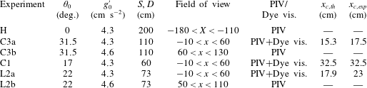
was varied in the experiments over two concave slopes of 60 cm and 110 cm, resulting in
 $\unicode[STIX]{x1D703}_{0}=17^{\circ }$
and
 $31.5^{\circ }$
respectively. On the concave wall, the slope angle
 $\unicode[STIX]{x1D703}$
varied from the maximum
 $\unicode[STIX]{x1D703}_{0}$
at the beginning of the slope to
 $0$
at
 $S$
(see figure 1). Additionally, one experiment over a linear slope with
 $\unicode[STIX]{x1D703}=22^{\circ }$
and a length of
 $S=73$
cm was performed. For each experiment C3, C1 and L2, at least three runs were conducted. Each run was analysed, and variations between them in the primary averaged quantities were less than 10 %, so that only results relative to one run for each experiment will be shown in this paper. The experimental conditions and measurement method are summarized in table 1. The
 $(X,Z)$
coordinate system represents horizontal and vertical directions, whereas
 $(x,z)$
represents the coordinate system relative to the inclined boundary, with the origin at the ridge (cf. figure 1).
Summary of the experimental parameters (
 $D\equiv$
length of horizontal channel upstream, C1 and C3 indicate concave slopes, L2 indicates a linear slope,
 $S\equiv$
slope length). The flow rate
 $0.6~\text{l}~\text{s}^{-1}$
and the total water depth in the channel
 $H_{0}=19$
cm were kept equal in all of the experiments. The overall and integral scale Reynolds numbers are
 $Re=3500$
and
 $Re_{{\mathcal{L}}}=66$
respectively.

To favour a uniform inflow, an inlet pipe facing upwards was installed at the bottom of the upstream section of the channel, and a plastic grid was positioned at the inlet to reduce interface fluctuations. The gravity current was generated by pumping salt water at a given density (
 $g^{\prime }=4.5~\text{cm}~\text{s}^{-2}$
) and flow rate (
 $Q=0.6~\text{l}~\text{s}^{-1}$
) from the first reservoir equipped with an electric agitator to maintain a uniform salt concentration. An adjustable pump with a maximum capacity of
 $2.5~\text{l}~\text{s}^{-1}$
was used to pump the salt water to the channel inlet via a rotameter so that flow rates could be recorded. The outlet was placed at the bottom of the downstream channel end to control the total water depth and allow discharge of the lower-layer salty flow.
Polyamide particles (Orgasol) with a mean diameter of
 $60~\unicode[STIX]{x03BC}\text{m}$
and a density of
 $1.016~\text{g}~\text{cm}^{-3}$
were added to both the salt and the fresh water as tracers for velocity measurements with particle image velocimetry (PIV). A 6 W argon-ion laser (Coherent) operating in multimode (
 $\unicode[STIX]{x1D706}_{1}=488$
nm,
 $\unicode[STIX]{x1D706}_{2}=514$
nm) was used as a continuous light source. The beam was transmitted through a fibre optic cable to a line generator with spherical lenses (OZ Optics). The generated laser sheet spanned a length of approximately 1 m, was of 5 mm thickness and was positioned in the middle of the channel. Images of 70 cm
 $\times$
50 cm were grabbed with a CCD camera (FlowMaster 3, 14 bit,
 $1400\times 1600$
pixels) at the maximal allowed frame rate of 23.84 Hz. With the use of an optical lens on the CCD camera, the spatial resolution was
 $0.435~\text{mm}~\text{pixel}^{-1}$
. With the software package DaVis (LaVision), the velocity fields were computed using a cross-correlation PIV algorithm. For this purpose, an adaptive multipass routine was used, starting with an interrogation window of
 $32\times 32$
pixels and a final window size of
 $16\times 16$
pixels, with
 $50\,\%$
overlap. Each vector of the resulting vector field represented an area of roughly
 $0.35~\text{cm}\times 0.35~\text{cm}$
. The velocity vectors were postprocessed using a local median filter. Given the velocities encountered in the experiments, the experimental error in the instantaneous velocity was estimated to be approximately
 $3\,\%$
and in
 $\unicode[STIX]{x2202}u/\unicode[STIX]{x2202}x$
approximately
 $10\,\%$
.
For dye visualizations, Rhodamine 6G was added to the dense (salt) water of the gravity current (experiments C3 and C1 in table 1). The dye visualizations were used to estimate the density profiles and some averaged values of the density field by normalizing locally with the maximal value.
4 Initial conditions: current on the flat bottom
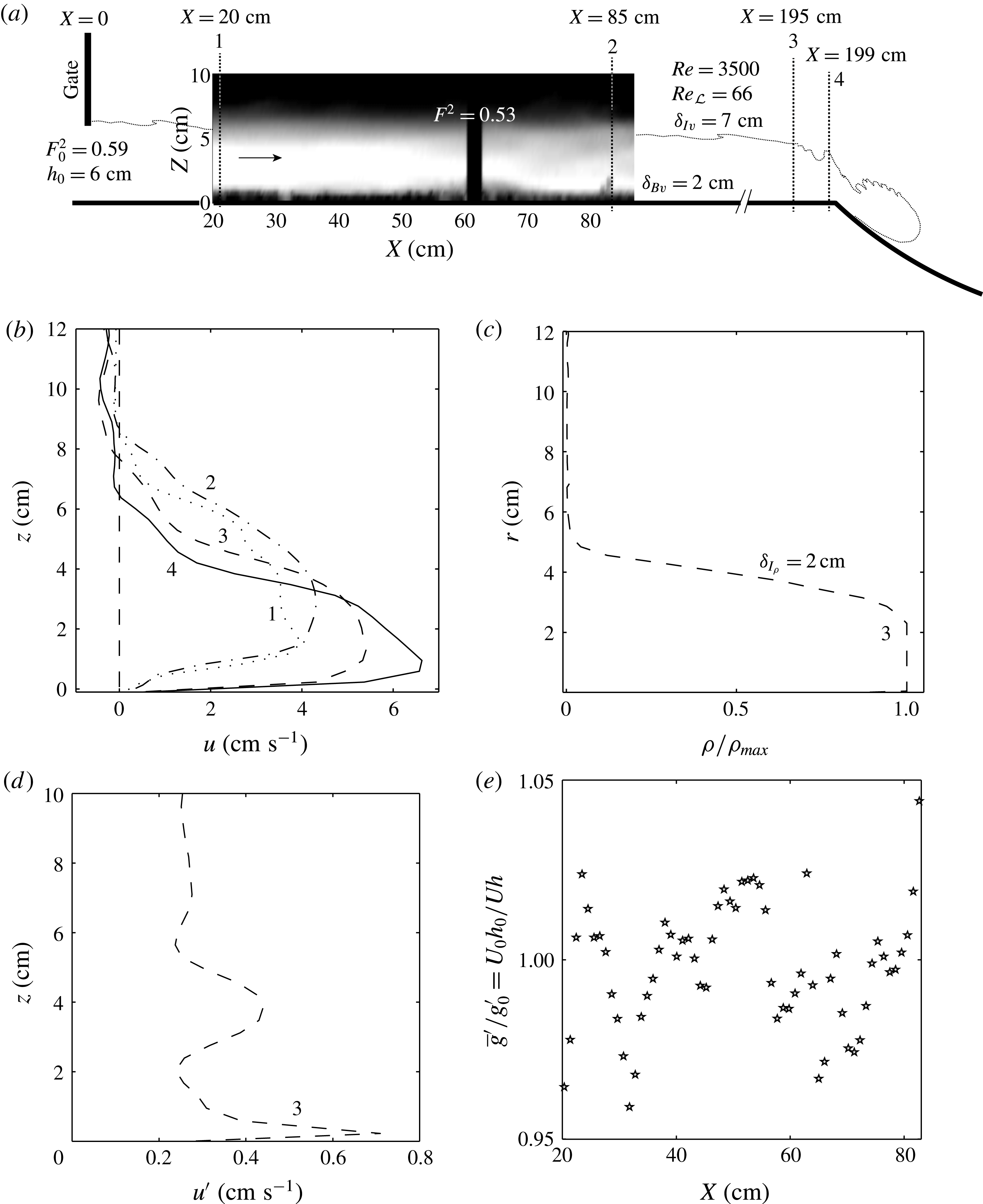
The current on the horizontal wall gives the initial conditions for the current on the slope (see figure 2
a). Using the experimental conditions as given in table 1, we estimate a Froude number at the gate of
 $F_{0}^{2}=q^{2}/(g_{0}^{\prime }h_{0}^{3})\approx 0.59$
for a gate opening of
 $h_{0}\approx 6$
cm and on the horizontal channel of
 $F^{2}=U/(g_{0}^{\prime }h)\approx 0.53$
using the data of figure 2. These values compare well with those given by Simpson (Reference Simpson1982) for a gravity current flowing along a horizontal surface for a depth ratio
 $h/H_{0}\approx 0.3$
.
Initial conditions of the gravity current flowing on the initial horizontal channel. (a) Time-averaged velocity field from PIV measurements (experiment H) displaying the initial conditions of the current. (b) Mean velocity profiles at
 $X=20$
(
 $\cdots \cdots$
),
 $85$
(–
 $\cdot$
), 195 (– –) and 199 cm (–) from the gate. (c) Vertical density profile obtained from the dye visualizations at
 $X=195$
cm from the gate. (d) Vertical profiles of the averaged (over time and all experiments) velocity fluctuations in the streamwise direction
 $u^{\prime }$
at
 $X=195$
cm. (e) Ratio between the streamwise buoyant acceleration normalized with the initial value on the initial horizontal channel, showing that it remains constant within
 $\pm 4\,\%$
fluctuations.

Very close to the slope change at
 $x=195$
cm downstream of the gate, the velocity and the current depth have reached
 $u_{m}\approx 6~\text{cm}~\text{s}^{-1}$
and
 $h\approx 6$
cm respectively, resulting in a bulk Reynolds number based on these scales of
 $Re=3500$
.
The expected boundary layer thickness at the end of the horizontal wall is
 $\unicode[STIX]{x1D6FF}_{B\unicode[STIX]{x1D708}}=5DRe_{D}^{-1/2}=3$
cm and the interface thickness is
 $\unicode[STIX]{x1D6FF}_{I\unicode[STIX]{x1D708}}\approx 8\sqrt{\unicode[STIX]{x1D708}t}$
(see Batchelor (Reference Batchelor1967), p. 188). Herein, the time is expressed using the distance
 $D=200$
cm (see figure 1) and the convective velocity estimated as half of the maximal velocity
 $U_{m}/2$
. This gives
 $\unicode[STIX]{x1D6FF}_{I\unicode[STIX]{x1D708}}\approx 11.3DRe_{D}^{-1/2}\approx 7.9$
cm. The density interface thickness is
 $\unicode[STIX]{x1D6FF}_{s}=\unicode[STIX]{x1D6FF}_{I\unicode[STIX]{x1D70C}}Sc^{-1/2}\approx 0.3$
cm, where
 $Sc$
is the Schmidt number, here close to 700.
Figure 2(b) displays velocity profiles at
 $X=20$
cm,
 $85$
cm, and two profiles very close to the ridge,
 $X=195$
cm and 199 cm from the gate (cf. also figure 2
a). With increasing distance, the shape of the profile approaches that of a wall jet. The boundary layer thickness, defined as the distance from the bottom where the velocity becomes 99 % of the maximal velocity, decreases after the initial adjustment close to the gate to
 $\unicode[STIX]{x1D6FF}_{B\unicode[STIX]{x1D708}}=2$
cm at 195 cm from the gate. The interface thickness is
 $\unicode[STIX]{x1D6FF}_{I\unicode[STIX]{x1D708}}=7$
cm at 195 cm from the gate. These values are in good agreement with those evaluated above.
The shape of the density profile can be estimated from the dye visualizations with Rhodamine 6G, and is displayed in figure 2(c) at 195 cm from the gate, showing a top-hat shape with a thin interface
 $\unicode[STIX]{x1D6FF}_{I\unicode[STIX]{x1D70C}}=2$
cm. This value is almost one order of magnitude larger than the value estimated from molecular diffusion only (
 ${\approx}0.3$
), but is still thin compared with
 $\unicode[STIX]{x1D6FF}_{I\unicode[STIX]{x1D708}}$
. The observation of Holmboe waves confirms the existence of a locally thin density compared with the shear interface.
We stress the fact that in our experiments, the interfacial Richardson number increases on the horizontal boundary according to
 $J\propto \unicode[STIX]{x1D6FF}_{I\unicode[STIX]{x1D708}}$
, and so the initial condition at the ridge is very different from that of previously performed gravity current experiments, as in Pawlak & Armi (Reference Pawlak and Armi2000), with already favourable conditions for the instability to develop due to a very thin
 $\unicode[STIX]{x1D6FF}_{I\unicode[STIX]{x1D708}}$
. Indeed, in our experiments,
 $\unicode[STIX]{x1D6FF}_{I\unicode[STIX]{x1D708}}=10$
cm at
 $x=10$
cm, compared with the
 $\unicode[STIX]{x1D6FF}_{I\unicode[STIX]{x1D708}}=1{-}2$
cm reported in the study of Pawlak & Armi (Reference Pawlak and Armi2000), so that the interface will become unstable only after a certain distance during the descent on the slope due to the increase of the velocity.
Figure 2(d) shows a vertical profile of the streamwise velocity fluctuations along the vertical direction typical for these experiments. Using
 $u^{\prime }\approx 0.5~\text{cm}~\text{s}^{-1}$
from the PIV measurements, an estimate for the integral-scale Reynolds number is given by
 $Re_{{\mathcal{L}}}=u^{\prime 2}\sqrt{15/(\unicode[STIX]{x1D708}\unicode[STIX]{x1D716})}\approx 66$
(the spatial resolution of the PIV of
 ${\sim}3~\text{mm}$
is very close to the Kolmogorov length scale
 $\unicode[STIX]{x1D702}_{K}=(\unicode[STIX]{x1D708}^{3}/\unicode[STIX]{x1D716})^{1/4}\sim O(1~\text{mm})$
, estimated using
 $\unicode[STIX]{x1D716}\sim u^{\prime 3}/h\sim 0.01~\text{cm}^{2}~\text{s}^{-3}$
(Tennekes & Lumley Reference Tennekes and Lumley1972)). This Reynolds number is high enough to assure a weakly turbulent flow.
The ratio
 $\overline{g}^{\prime }/g_{0}^{\prime }=q_{0}/(Uh)$
along the flow direction is plotted in figure 2(e). It remains constant along the horizontal wall within
 $\pm 4\,\%$
variations, showing that entrainment is negligible there.
5 Currents on the concave bottom
Approximately 50 s after opening the gate, the head of the current reaches the slope. Similarly to a potential flow over a weir, acceleration starts already approximately 10 cm before the ridge, as is evident from the fast increase in velocities over the short distance of 4 cm (195–199 cm from the gate in figure 2
a). Although the slope change is abrupt from horizontal (
 $\unicode[STIX]{x1D703}=0$
) to
 $\unicode[STIX]{x1D703}_{0}$
, the streamlines do not follow the abrupt change of bottom but are curved like in potential flow.
After an initial unsteady phase with the passage of the gravity current head, a steady two-layer flow establishes with an internal hydraulic control
 $F=1$
at the ridge (Armi Reference Armi1986) and a supercritical flow (
 $F>1$
) on the slope. Once the current has terminated the descent, it may return again to subcritical conditions, passing through an internal hydraulic jump or spreading out smoothly. On a straight slope that returns abruptly to the horizontal, an internal hydraulic jump is expected, but on the concave slope, a smooth transition seems to take place. This will be investigated elsewhere.
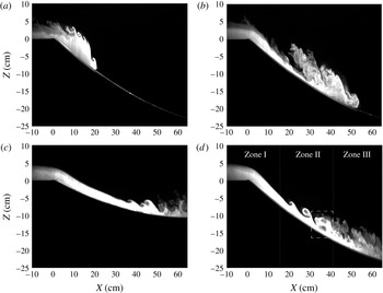
Instantaneous images from dye visualizations of (a,b) the head descending the slope from experiment C3 with time intervals of
 $4$
and
 $6$
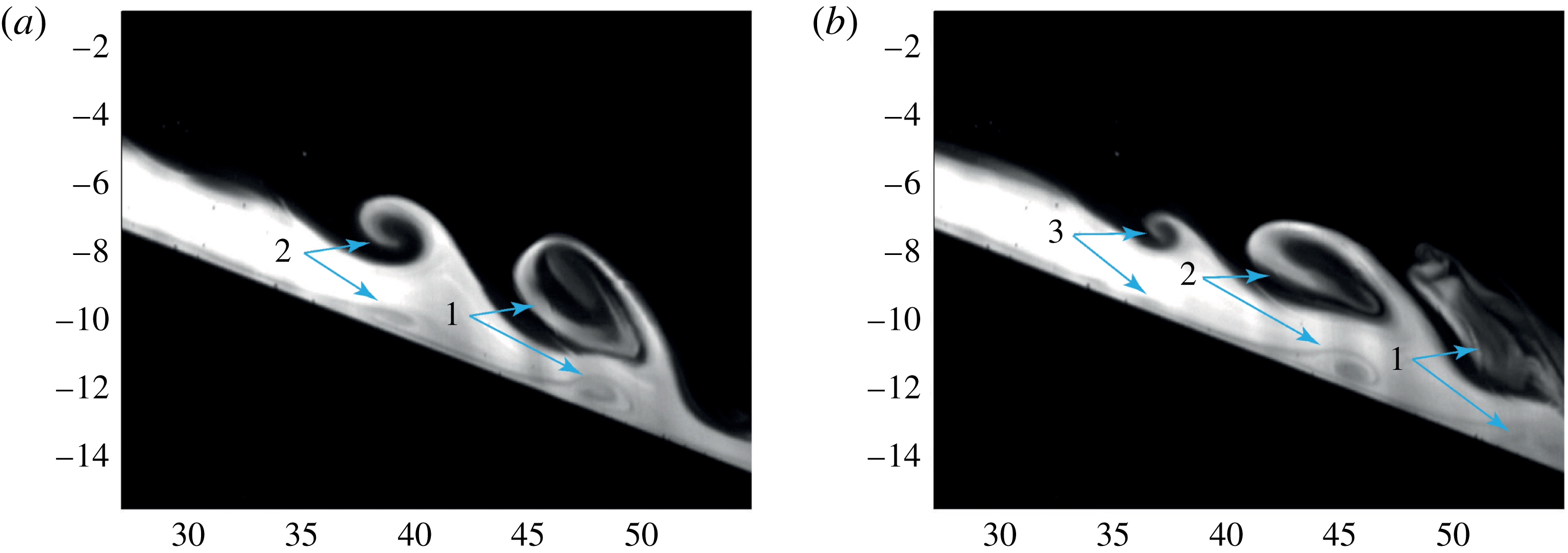
s, and of the steady current in experiments C1 (c) and C3 (d) taken 100 s after the gate opening. The vertical scale of the images is approximately 35 cm, while the horizontal scale is approximately 70 cm. As depicted in (d), three zones can be defined: the initial stable interface region with no entrainment, the central region with KH instabilities and the final region of collapse to a turbulent shear layer. The dashed rectangle in (d) highlights the boundary layer separation coupled with a KH billow which will be discussed in §§ 5.2 and 6.

Figure 3 shows dye visualizations of the steady flow for the experiments C1 (c) and C3 (d) with a concave slope. As depicted in figure 3(d), we can distinguish three zones during the steady phase. The first zone (zone I) is characterized by a strong initial acceleration of the flow and a reduction of the layer depth with relatively thin velocity and density shear layers and a stable interface with respect to the KH instability. The intermediate zone (zone II) is characterized by the onset of KH billows due to the increased velocity shear which cause significant entrainment of upper-layer fluid into the lower layer. The final zone (zone III) is characterized by the collapse of the KH billows which generate an intermediate upper layer with an intermediate density. As is evident from figures 3(c) and 3(d), a significant change in the development of the interfacial shear layer occurs during the descent down the slope. In zone III, the stratified shear layer collapses and subsequently restratifies, which is a well-documented process examined by Koop & Browand (Reference Koop and Browand1979) (see also, e.g., Corcos & Sherman (Reference Corcos and Sherman1976)). They observed an initial rapid growth through vortex pairing of the shear layer, and as the Richardson number increased past a critical value, the pairing mechanism was suppressed, the development of the layer ceased and production of turbulence in the shear layer died out, with the exception of turbulence generated by the restratification process. When the slope angle at this location is still high enough, the current accelerates and the Richardson number will drop again to unstable values so that further mixing can occur within the already restratified shear layer.
We observed that during one experiment the limits between these three zones slowly shift upstream. Indeed, with time the density increases in the lower part of the upper layer and so does the return flow caused by the strong dilution in zone III. Kelvin–Helmholtz billows can thus appear further upstream for lower velocities.
Two ranges of acceleration have been considered by varying the initial concave slope angle
 $\unicode[STIX]{x1D703}_{0}$
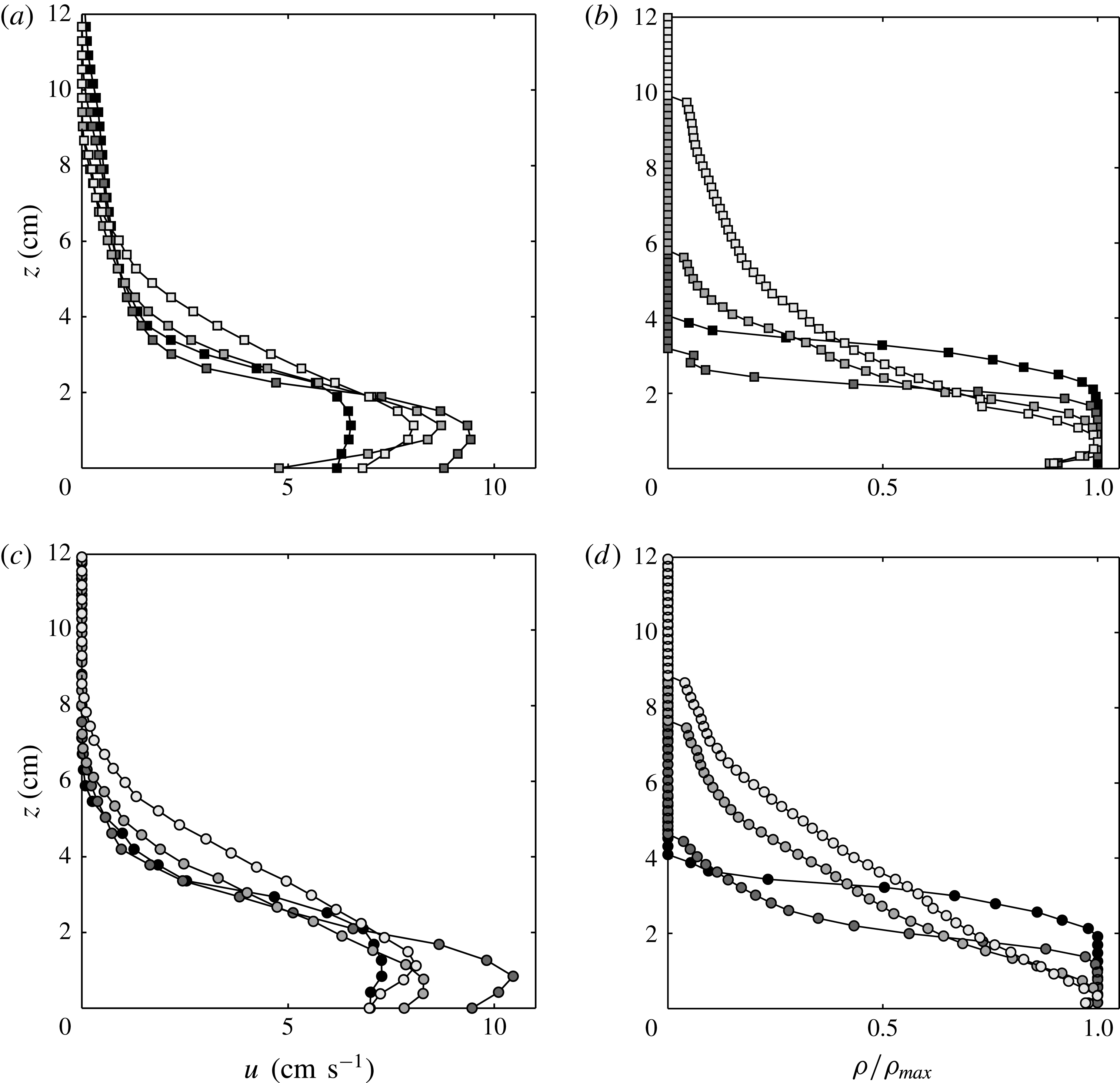
, as described in § 3. Time-averaged velocity (a,c) and density (b,d) profiles at four different downstream positions (
 $x=3$
cm,
 $x=22$
cm,
 $x=35$
cm,
 $x=57$
cm) are plotted in figure 4 for the experiments C1 (a,b) and C3 (c,d). These sections are characteristic of the three zones I, II and III discussed above, with the latter two profiles being at the beginning and at the end of zone III. We see that initially the velocity increases at the beginning and the profile approaches that of a wall jet, and smooths subsequently in zone III. Density profiles (see figure 4 for experiments C1 (b) and C3 (d)) relative to the maximal value are stepwise at the beginning of the descent and smooth, similarly to the velocity profiles, while moving down the slope.
In the following sections, we will present time-averaged quantities versus the downstream position measured from the ridge. This average is made over 65 s, from
 $t=20$
s after gate opening, excluding thus the initial passage of the head, until
 $t=85$
s. Results are presented for the two concave slopes, first for experiment C1 with a smoother transition on the slope and then increasing the initial slope angle as for experiment C3. For comparison, a linear sloping boundary is used in § 6. These quantities are not non-dimensionalized as is customary for shear flows, since there is no single non-dimensional parameter for downstream distance in a spatially accelerating flow.
Time-averaged velocity (a,c) and density (b,d) profiles at
 $x=3$
cm,
 $x=25$
cm,
 $x=43$
cm and
 $x=57$
cm (from dark to light grey respectively) from the ridge for experiment C1 (a,b) and for experiment C3 (c,d).

5.1 Smooth transition on a concave slope
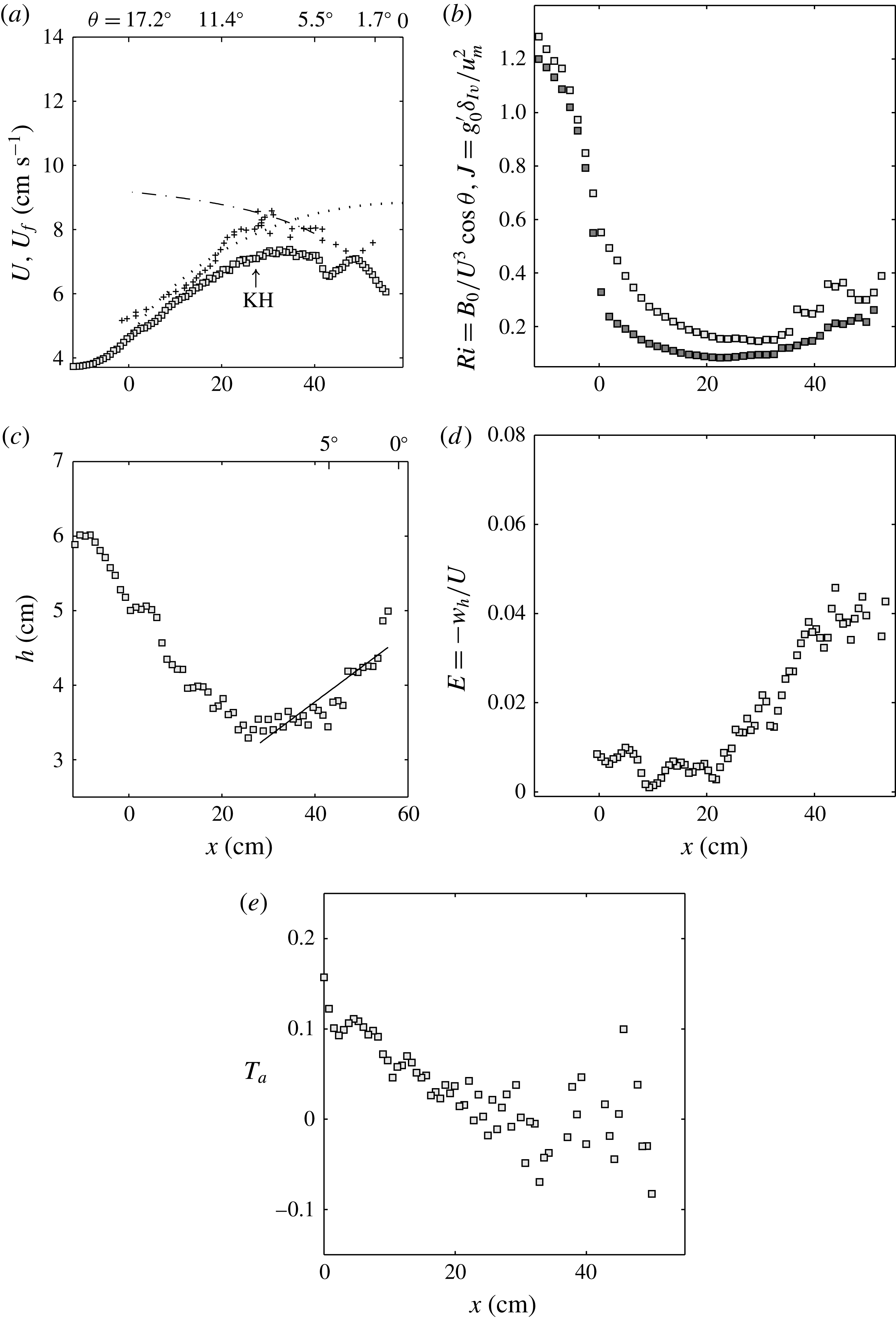
Figure 5(a) displays for the smaller slope of experiment C1 the depth-integrated quantities and then averaged in time, with the velocity of the gravity current head indicated by the symbols
 $(+)$
, and (▫) for the depth-integrated velocity after the passage of the gravity current head. Both are obtained from the PIV measurements. In agreement with former observations (Britter & Linden Reference Britter and Linden1980), the velocity of the gravity current head derived from the positions of maximum velocity in the current at each instant increases steadily to reach an equilibrium value. The free fall velocity is indicated for comparison and is given by
 $$\begin{eqnarray}U_{free}=\sqrt{2S_{2}Rg_{0}^{\prime }(\cos \unicode[STIX]{x1D703}_{0}-\cos \unicode[STIX]{x1D703})+U_{0}^{2}},\end{eqnarray}$$
where
 $U_{0}^{2}$
is the velocity at the ridge,
 $x=0$
.
Time-averaged quantities for experiment C1 versus
 $x$
. (a) Depth-integrated velocity (▫) in comparison with (2.11) (— ⋅ —),
 $c_{D}=2\times 10^{-3}$
and
 $E=9\times 10^{-4}(5+\unicode[STIX]{x1D703})$
; (
 $\cdots \cdots$
) free fall solution (5.1) neglecting friction and pressure variations; head velocity (
 $+$
). (b) Richardson numbers
 $Ri$
(▫) and
 $J$
(▪). (c) Current depth
 $h$
(symbols) fitted with a linear relation where
 $\text{d}h/\text{d}x=0.047$
(–). (d) Entrainment coefficients
 $E=-w_{h}/U$
. (e) Acceleration parameter
 $T_{a}=(h/U)\,\text{d}U/\text{d}x$
.

The flow behind the head ((▫) in figure 5
a) first accelerates until
 $x\approx 31$
cm, which corresponds approximately to the location where KH billows first develop. Then, the velocity decreases slightly after a passage at a maximal value of
 $7.7~\text{cm}~\text{s}^{-1}$
. This maximal velocity value is very close to the quasiequilibrium-state velocity of
 $8.2~\text{cm}~\text{s}^{-1}$
. At
 $x>50$
cm, the flow has reached the end of the slope to attain eventually the gravity wave speed
 ${\approx}\sqrt{\overline{g^{\prime }}h/2}$
. The quasiequilibrium state, defined by the driving buoyancy force being in balance with the total friction and here obtained after substituting the measured velocities in (2.11) (dash-dotted line in figure 5
a), seems to be reached only between
 $x=31$
and 50 cm. Here, the entrainment law from Turner (Reference Turner1973) has been used, with
 $E=\text{d}h/\text{d}x\approx 9\times 10^{-4}(5+\unicode[STIX]{x1D703}^{\circ })$
, corresponding to
 $\unicode[STIX]{x1D703}>5^{\circ }$
. We notice that this depth-integrated velocity follows the head velocity discussed above until approximately
 $x<20$
cm. Then, the head velocity continues to increase and reaches the curve of the equilibrium-state velocity (Ellison & Turner Reference Ellison and Turner1959) at approximately
 $x>30$
cm.
We define the Richardson number
 $Ri=\overline{g^{\prime }}h\cos \unicode[STIX]{x1D703}/U^{2}$
in terms of the buoyancy flux
 $B$
, which is conserved (equal to
 $B_{0}$
) and constant along the flow direction so that
 $Ri=B_{0}\cos \unicode[STIX]{x1D703}/U^{3}$
. It should be noted that
 $U$
and
 $h$
are the depth-integrated velocity and current height determined from (2.7b
) and
 $\overline{g^{\prime }}=B_{0}/(Uh)$
. The variation of the bulk Richardson number
 $Ri$
along the downstream direction for experiment C1 is shown in figure 5(b). We see that the values are large at the beginning, suggesting that the interface is KH stable, as is also observed from dye visualizations. Due to the flow acceleration,
 $Ri$
decreases rapidly and reaches a value of
 $Ri\approx 0.15$
at
 $x\approx 30$
cm. In this region, we observe KH billows causing the entrainment, reducing the velocity and decreasing the density difference, so that
 $Ri$
increases again up to
 $0.4$
. Close to the slope end for
 $x>40$
cm, we see some more intermittent KH-like upwellings very different from the rolling up KH billows observed during the first passage to an unstable interface in zone II. We note that the flow remains supercritical over all of the slope length and the Froude number defined as
 $F=1/\sqrt{Ri}>1.5$
(cf. figure 5
b). In figure 5(b), we plot also for comparison the interfacial Richardson number
 $J$
(dark symbols) defined with the shear layer thickness,
 $J=\overline{g^{\prime }}\unicode[STIX]{x1D6FF}_{I\unicode[STIX]{x1D708}}/u_{m}^{2}$
, and see that, except that the values are lower, the behaviour is the same as for the bulk Richardson number
 $Ri$
.
The downstream variation of the time-averaged current depth
 $h$
is plotted in figure 5(c). First, the current depth decreases due to the acceleration down the slope, and then for
 $x>35$
cm it starts to increase due to interfacial instabilities.
The entrainment rate is defined as
 $$\begin{eqnarray}E=\frac{1}{U}\frac{\text{d}Uh}{\text{d}x}=\frac{\text{d}h}{\text{d}x}+\frac{h}{U}\frac{\text{d}U}{\text{d}x}=\frac{\text{d}h}{\text{d}x}+T_{a}.\end{eqnarray}$$
Equation (5.2) highlights that the entrainment
 $E$
can be expressed in terms of the rate of change in current depth
 $\text{d}h/\text{d}x$
and the rate of change in velocity
 $(h/U)(\text{d}U/\text{d}x)$
, i.e. an acceleration parameter. For a current in equilibrium with a constant velocity, the total entrainment is given by
 $\text{d}h/\text{d}x$
only, which represents then the angle of spread of the interface with respect to the bottom boundary (Morton, Taylor & Turner Reference Morton, Taylor and Turner1956). This angle of spread is constant for a developed current on a constant slope and, following the relation
 $\text{d}h/\text{d}x=9\times 10^{-4}(5+\unicode[STIX]{x1D703})$
, as obtained by fitting the data of Ellison & Turner (Reference Ellison and Turner1959), depends on the slope angle only. The acceleration parameter
 $T_{a}$
gives the contribution to the rate of change in volume flux, and thus to entrainment, due to the variation of the velocity
 $U$
on the slope. We note that even when the interface is stable and no entrainment occurs, this definition is still valid: the positive acceleration contribution
 $T_{a}>0$
before onset of the KH instability is then balanced by a negative inclination of the interface with respect to the bottom, i.e.
 $\text{d}h/\text{d}x<0$
.
Equation (5.2) shows that
 $T_{a}$
can be calculated from the velocity gradients as defined in § 2 (see (2.9)), but also from the entrainment rates, i.e.
 $T_{a}=(h/U)\,\text{d}U/\text{d}x=E-\text{d}h/\text{d}x$
, where
 $E$
is the ‘total’ entrainment rate resulting from both contributions on the right-hand side of (5.2), and which can be expressed also in terms of the velocity
 $w_{h}$
normal to the interface (Morton et al.
Reference Morton, Taylor and Turner1956), i.e.
 $$\begin{eqnarray}E=-\frac{w_{h}}{U}.\end{eqnarray}$$
This enables different ways to calculate the entrainment rates
 $E$
and the acceleration parameter
 $T_{a}$
. As is evident from (5.2), the determination of
 $E$
relies on gradient estimates. A direct calculation of these gradients from experimental data leads to large errors and hence is difficult to interpret, as in the case of the acceleration parameter
 $T_{a}=(h/U)\,\text{d}U/\text{d}x$
. A primary source of error in these gradient estimates which are related to the volume flux results from the slow downstream variation of the onset of KH instabilities. The initial point of finite-amplitude development in each experiment varied over a range of approximately
 ${\approx}10$
cm during an experiment of approximately 2 min. To avoid these difficulties, the total entrainment rates have been estimated using (5.3), where the velocities
 $w_{h}$
and
 $U$
are obtained from the PIV measurements. The velocity
 $w_{h}$
has been computed by taking the time-averaged velocity field, decomposing the
 $u$
and
 $w$
components of the PIV velocities in the normal direction of the interface, the inclination of which corresponds to the streamline curvature inclination, and then taking the average between the value at the interface and the value above and below the interface location.
The experimental entrainment rates for experiment C1 are plotted in figure 5(d), where the symbols represent
 $E=-w_{h}/U$
. Entrainment rates are practically zero during the acceleration phase and increase rapidly as KH billows develop to reach the maximal values for
 $x\geqslant 40$
cm. The continuous line in figure 5(c) enables us to estimate the entrainment contribution from the interface inclination, which represents a linear fit with
 $\text{d}h/\text{d}x=0.045$
. The linear fit, however, seems to better predict the final maximal values of the entrainment rates for
 $x>40$
cm, being around
 $E=0.04$
(cf. figure 5
d), while the relation (2.12) underestimates these values by a factor of 4.
In figure 6(e), the acceleration parameter
 $T_{a}=(h/U)\,\text{d}U/\text{d}x$
is plotted versus the downstream direction for experiment C1. It can be stated that its magnitudes for
 $x<20$
cm are around
 $0.1$
and the location at which
 $T_{a}$
is around zero is at onset of KH instability, i.e.
 $x\approx 30$
cm. We see in general that in the region in which
 $T_{a}$
is large, the time scale proportional to
 $h/U$
related to the overturning in the shear layer is much smaller.
5.2 Larger slope change
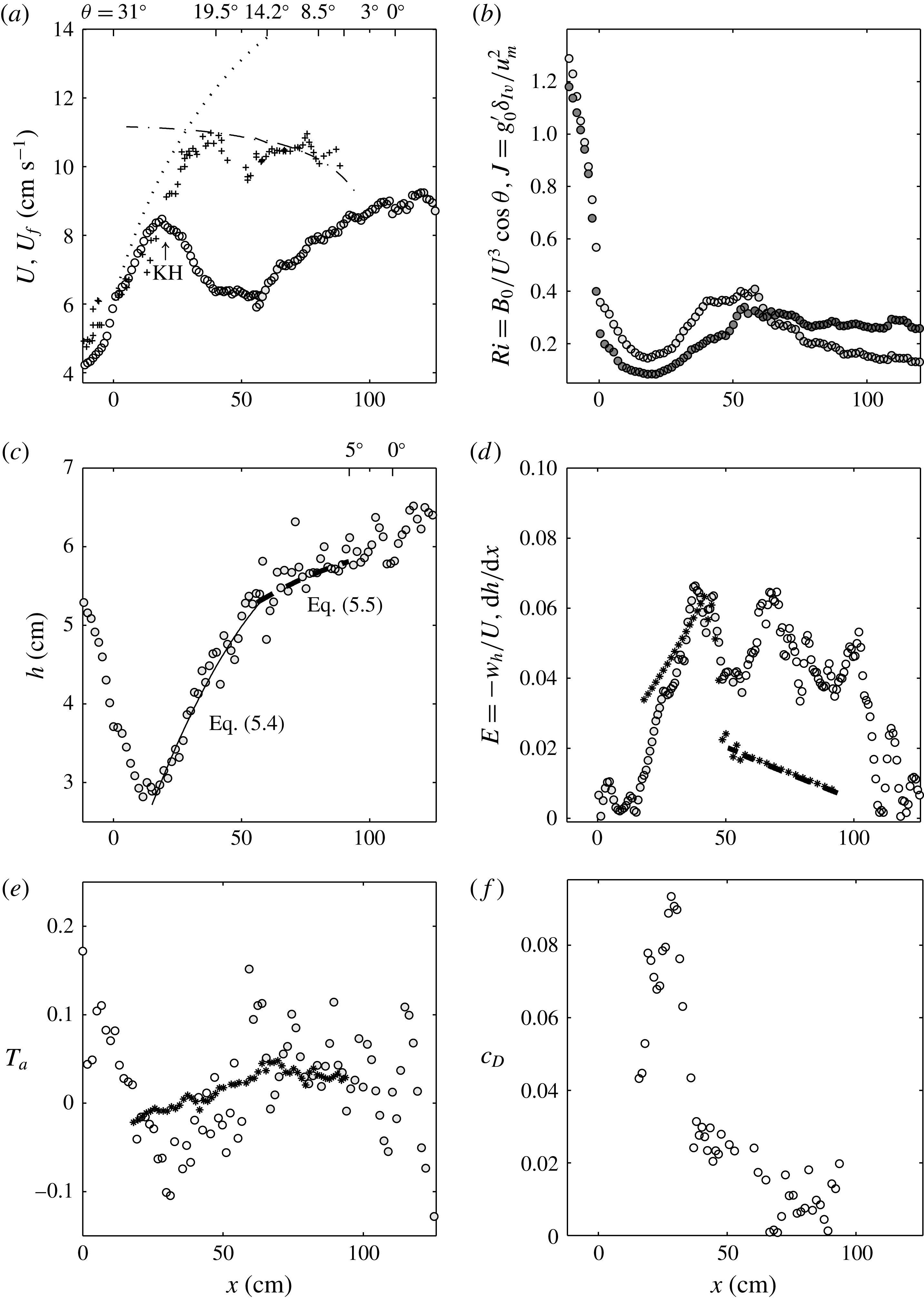
Figure 6(a) shows the velocity of the head (
 $+$
) and the depth-integrated layer velocity for experiment C3, where the initial slope angle is
 $\unicode[STIX]{x1D703}_{0}=31.5^{\circ }$
. The free fall velocity (dotted line) is slightly larger than these velocities. The depth-integrated velocity (
 $U$
) reaches a maximum at
 $x\approx 17.5$
cm, whereas the head velocity continues to increase until it reaches the equilibrium state velocity when
 $x>40$
cm. The maximum of
 $U$
corresponds approximately to the location where KH billows first develop. In zone II, the velocity decreases due to interfacial and bottom friction. After a readjustment, the velocity starts to increase again at
 $x\approx 50$
cm, where the slope is still
 $16^{\circ }$
. At
 $x=115$
cm (
 $\unicode[STIX]{x1D703}=0$
), the velocity has a value of
 $9~\text{cm}~\text{s}^{-1}$
. At this location, where the flow has reached the end of the slope, it is expected to decelerate to a velocity
 ${\approx}\sqrt{\overline{g^{\prime }}h/2}$
.
This gravity current is different from that observed in experiment C1 and those normally described in previous studies in that it passes through acceleration–deceleration cycles so that the equilibrium state of roughly
 $10{-}11~\text{cm}~\text{s}^{-1}$
, as represented by (2.11), is never reached. This is highlighted by comparing the measured velocities (○) with the dash-dotted line in figure 6(a) expressing (2.11). Video recordings revealed that this acceleration–deceleration is often associated with the merging of several KH billows into one large billow that makes the bottom layer flow almost disappear. As a consequence, interfacial entrainment and bottom drag increase considerably. The flow then needs some time (and distance) to adjust and eventually accelerate again. For this experiment, the deceleration is sudden, related to a violent onset of the KH billows. In experiment C1, the acceleration is more gentle and thus also the onset of the interfacial instabilities; in this case, there is only one acceleration phase in which the current reaches a maximal velocity very close to the equilibrium state velocity and the flow decelerates as it reaches the horizontal boundary. In experiment C3, we see that the gravity flow constantly changes its velocity over a length of 120 cm before reaching the horizontal bottom.
Time-averaged quantities for experiment C3 versus
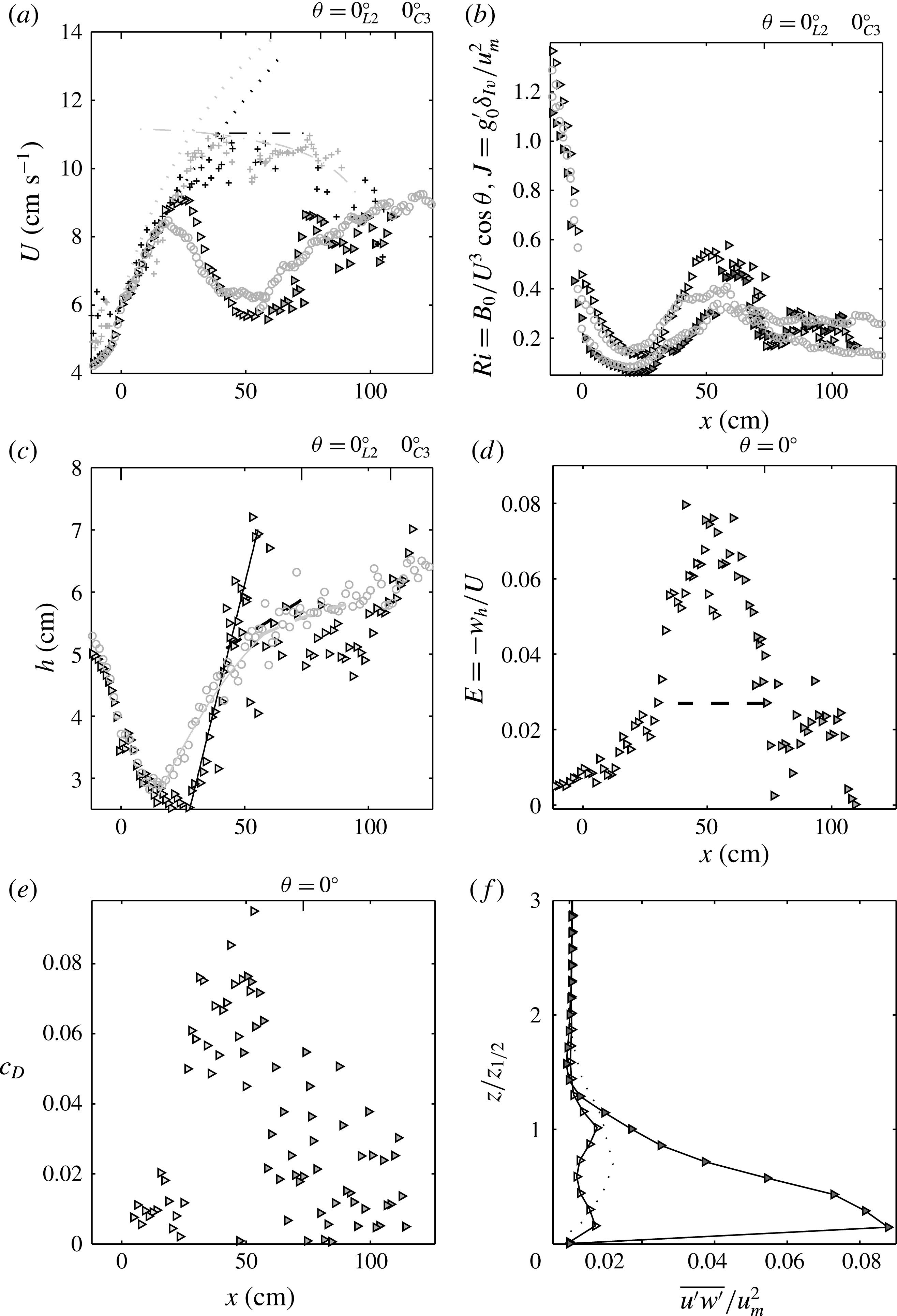
 $x$
. (a) Depth-integrated velocity (○); equilibrium velocity (2.11) (— ⋅ —) with
 $c_{D}=2\times 10^{-3}$
and
 $E=9\times 10^{-4}~(5+\unicode[STIX]{x1D703})$
; (
 $\cdots \cdots$
) free fall solution (5.1); head velocity (
 $+$
). (b) Richardson numbers
 $Ri$
(○) and
 $J$
(●). (c) Current height
 $h$
(○) fitted with (5.4) (–) and (5.5) (– –). (d) Entrainment coefficients
 $E=-w_{h}/U$
(symbols) and
 $\text{d}h/\text{d}x$
(*) from experimental data fitted with the parabolic relations (5.4) and (5.5); (– –)
 $E=9\times 10^{-4}(5+\unicode[STIX]{x1D703})$
. (e) Acceleration parameter
 $T_{a}=(h/U)\,\text{d}U/\text{d}x$
(
 $\circ$
) and
 $T_{a}=w_{h}/U-\text{d}h/\text{d}x$
(*), where
 $\text{d}h/\text{d}x=9\times 10^{-4}(5+\unicode[STIX]{x1D703})$
. (f) Drag coefficient
 $c_{D}$
determined from (2.9) using
 $T_{a}=w_{h}/U-\text{d}h/\text{d}x$
.

The Richardson numbers
 $Ri$
and
 $J$
are plotted in figure 6(b), with empty and filled symbols respectively. We see that both decrease rapidly to
 $0.2$
or less in the first accelerating region and then both increase as KH billows develop. In this experiment however, the overall interfacial Richardson number reaches a final value of
 $J\approx 0.25$
, while the overall
 $Ri$
decreases again for
 $x>55$
cm to a smaller value of
 ${\approx}0.15$
.
Figure 6(c) displays the downstream variation of the current depth
 $h$
. After an initial decrease due to the acceleration of the flow up to approximately 20 cm, for
 $x>20$
cm, the current depth
 $h$
can be approximated by the parabolic relation
 $$\begin{eqnarray}h(x)=-5.4\times 10^{-4}x^{2}+0.1x+1.3,\end{eqnarray}$$
while for
 $x>55$
cm it is closer to the parabolic relation
 $$\begin{eqnarray}h(x)=9\times 10^{-4}[(5+S/R\unicode[STIX]{x03C0}/180)x-x^{2}/(2R)]+h_{I}.\end{eqnarray}$$
Expression (5.5) corresponds to integration of the equation
 $\text{d}h/\text{d}x=9\times 10^{-4}(\unicode[STIX]{x1D703}+5)$
, where
 $h_{I}$
is the integration constant, which is determined from the initial condition given by the experimental data,
 $h_{I}=4.5$
cm. The use of the parabolic relation (5.4) for
 $20~\text{cm}<x<55$
cm highlights how different the coefficients of the parabola are compared with those given in (5.5), which would thus underestimate the increase of the current depth.
The experimental entrainment rates for experiment C3 are plotted in figure 6(d), where empty symbols (○) represent
 $E=-w_{h}/U$
and the (
 $\star$
) symbols
 $\text{d}h/\text{d}x$
; the values of
 $\text{d}h/\text{d}x$
have been obtained from the parabolic fits (5.4) and (5.5) when
 $50~\text{cm}<x<90$
cm shown in figure 6(b). The total entrainment rate
 $E$
attains a maximum of
 $0.07$
at the end of the first deceleration (
 $40<x<50$
). After a short nearly constant velocity, the current reaccelerates again when it enters zone III, and
 $E$
reaches again a value of
 ${\approx}0.07$
. We see that for
 $x<30$
cm, the term
 $\text{d}h/\text{d}x$
is larger than the total entrainment rate
 $E$
because the acceleration parameter is negative (cf. (5.2) and figure 6
c). For
 $40~\text{cm}<x<55$
cm, the two terms are very similar as the acceleration parameter is close to zero. Then, for
 $x>55$
cm,
 $\text{d}h/\text{d}x$
follows the empirical linear relation
 $\text{d}h/\text{d}x=9\times 10^{-4}(5+\unicode[STIX]{x1D703})$
, so that the total entrainment becomes larger due to the contribution of the flow acceleration.
In figure 6(e), the acceleration parameter
 $T_{a}$
is plotted, with the empty symbols (○) representing the values calculated from the horizontal velocity gradients, i.e.
 $T_{a}=(h/U)\,\text{d}U/\text{d}x$
, and the (
 $\star$
) symbols representing
 $T_{a}=E-\text{d}h/\text{d}x$
(cf. (5.2)), with
 $E$
being determined from local velocity values, with (5.3). The relatively important scatter for
 $x>20$
cm in
 $T_{a}$
with magnitudes varying between
 $-0.08$
and
 $0.1$
is due to the KH billows that start at the location
 $x>20$
cm. Nevertheless, the corresponding location of
 $T_{a}\sim 0$
is well captured, and so are the deceleration–acceleration regions for
 $x>20$
cm.
For this experiment C3, we made a more detailed estimation of the errors and so we considered the time-averaged velocity field over 2000 images. We took then the
 $3\,\%$
error estimated from the PIV measurements for each velocity and assumed a Gaussian distribution of the errors, independent from each other. After 2000 random selections per final interrogation window, the typical errorbar on the estimation of
 $U$
and
 $h$
over the full selection of 2000 has been determined: the absolute error is less than 1 % for
 $U$
and
 $h$
for 80 % of the velocities, and a relative error of less than 3 % and 5 %, for
 $U$
and
 $h$
respectively. For
 $\text{d}h/\text{d}x$
and
 $T_{a}$
, which are more affected by the error of the input velocities, we obtain that for approximately 40 % of them the relative error is less than
 $100\,\%$
; however,
 $50\,\%$
of the absolute errors for
 $\text{d}h/\text{d}x$
and
 $T_{a}$
are less than
 $5\,\%$
. Herein, the spatial derivatives have been calculated for each time step.
In order to better explain this process of strong deceleration and reacceleration, we consider the bottom friction coefficient, because entrainment only may not be sufficient to cause such a slowdown of the current. An estimation of the bottom friction coefficient
 $(c_{D})$
is obtained by rearranging (2.9) in the form
 $$\begin{eqnarray}c_{D}={\displaystyle \frac{{\mathcal{S}}_{2}\sin \unicode[STIX]{x1D703}}{U^{3}/B}}-T_{a}\left(1+\frac{1}{2}{\mathcal{S}}_{1}Ri\right)-\frac{1}{2}{\mathcal{S}}_{1}h\frac{\text{d}Ri}{\text{d}x}-E,\end{eqnarray}$$
where the acceleration term,
 $T_{a}$
, and the change in
 $Ri$
are determined from the experiments. The extrapolated total friction coefficient (5.6) is plotted in figure 6(f), with the symbols (○) being obtained with the velocity gradients
 $T_{a}=(h/U)\,\text{d}U/\text{d}x$
.
The data displayed in the figure demonstrate that the bottom friction coefficient must be very large, i.e. of order
 ${\approx}10^{-1}$
(figure 6
f). This is beside any source of experimental error, as for instance the power of 3 of the velocity in (5.6), the difficulties in determining
 $T_{a}$
and the gradients of
 $\text{d}Ri/\text{d}x$
. Similar observations have also been reported in the numerical study of Ross, Dalziel & Linden (Reference Ross, Dalziel and Linden2006).
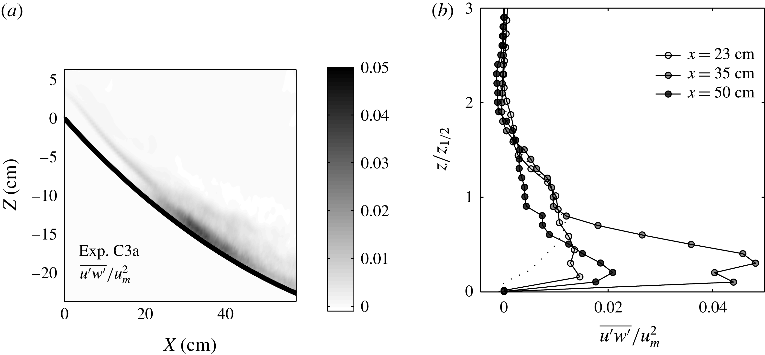
Reynolds stresses
 $\overline{u^{\prime }w^{\prime }}$
normalized with the maximal velocity
 $u_{m}^{2}$
. Overall field (a) and selected vertical velocity profiles (b) at three
 $x$
positions on the concave slope C3; (
 $\cdots \cdots$
) plane wall jet from Zhou, Heine & Wygnanski (Reference Zhou, Heine and Wygnanski1996).

To support this statement of large bottom friction, we evaluate
 $c_{D}$
also from the velocity fluctuations in the boundary layer. For this experiment, the Reynolds stress, normalized with the local maximal velocity
 $\overline{u^{\prime }w^{\prime }}/u_{m}^{2}$
, is presented in figure 7(a,b). In figure 7(b), the vertical scale is normalized with the height
 $z_{1/2}$
at which the velocity is half of the maximal velocity. For comparison, the dotted line represents the measured values from Zhou et al. (Reference Zhou, Heine and Wygnanski1996) and shows that our Reynolds stress is relatively large, reaching
 $5\,\%$
of the maximal velocity with the maximal value relatively close to the bottom boundary. From figure 7(b), we estimate
 $c_{D}=\overline{u^{\prime }w^{\prime }}/U^{2}\approx 0.1$
, using
 $u_{m}=1.4U$
from the experimental data, which compares well with the maximum value displayed at the same location
 $x=35$
cm in figure 6(f).
The comparison between the values of
 $c_{D}$
obtained in figure 6(f) and the local high Reynolds stress for
 $20<x<40$
reported in figure 7, as well as the visual observation of the development of bottom billows in the boundary layer coupled with the development of the KH billows at the interface, are all supporting arguments that verify the statement of a large bottom drag
 $c_{D}$
. Together with the large entrainment
 $E$
at the interface, these explain the sudden deceleration of the flow and therewith its atypical behaviour with respect to previous results. In experiment C1, the entrainment rates were half of those reported for experiment C3 and also the estimated bottom friction coefficient
 $c_{D}$
was one order of magnitude less, with Reynolds stresses reaching only 1.5 % maximum of the square of the maximal velocity
 $u_{m}^{2}$
.
Series of zoomed views of the current at onset of KH instability. Dye visualizations of experiment L2 with a time interval of 0.5 s, showing the development of large bottom billows coupled with the development of the overlying KH billows. The approximate length scale of these boundary billows is 1 cm.

6 Comparison with steep straight slopes
Time-averaged quantities for experiment L2. (a) Variation of the depth-integrated velocity compared with the predictions of (2.11) (— ⋅ —); (
 $\cdots \cdots$
) free fall solution; head velocity (
 $+$
). (b) Richardson numbers
 $Ri$
( ▹) and
 $J$
( ▸). (c) Current depth
 $h$
fitted with
 $\text{d}h/\text{d}x=0.1631$
for
 $20~\text{cm}<x<55$
cm (–) and the relation of Ellison & Turner (Reference Ellison and Turner1959),
 $\text{d}h/\text{d}x=0.025$
(– –). The data for experiment C3 in (a–c) are shown in light grey. (d) Entrainment coefficients
 $E=-w_{h}/U$
, (– –)
 $E=9(5+\unicode[STIX]{x1D703})\times 10^{-4}$
. (e) Bottom friction
 $(c_{D})$
determined from (2.9) using experimental data. (f) Selected vertical velocity profiles at
 $x=23$
cm (empty symbols) and
 $x=35$
cm (filled symbols); (
 $\cdots \cdots$
) plane wall jet from Zhou et al. (Reference Zhou, Heine and Wygnanski1996).

Curved slopes start steep and then rapidly decrease in steepness to the horizontal plane. The observations above suggest that the strong acceleration at the ridge leads to the formation of KH billows and a related large increase in the entrainment rate
 $E$
and drag
 $c_{D}$
, whereas the downhill deceleration seems to have no influence. In order to confirm that it is indeed only the steep part of the slope that determines the essential part of the downslope dynamics, we consider a gravity current on a steep but straight slope of comparable steepness. For comparison, we superimposed in figure 9(a–c) the velocity, Richardson numbers and current depth variations obtained on straight slopes on those obtained on concave slopes. It is seen that the spatial development of the current on the linear slope is qualitatively similar to that observed on the concave bottom in experiment C3 with an abrupt topography change. As described in § 5, the three zones of first acceleration of the flow (zone I), development of KH billows (zone II) and their subsequent collapse (zone III) are also found here. A close-up view of the onset and development of KH billows (zone II) is shown in figure 8. There is a strong effect of the KH instability on the bottom boundary layer. Moreover, the averaged flow quantities for the straight slope (experiment L2) shown in figure 9 are similar to those for the concave slope (experiment C3), with the head velocity (
 $+$
symbols in figure 9
a) increasing steadily until they reach roughly the constant equilibrium-state velocity and then dropping off when the horizontal bottom is reached. Detailed comparison shows that the depth-integrated velocity (figure 9
a) increases rapidly up to a maximal velocity of
 $9~\text{cm}~\text{s}^{-1}$
at
 $x\approx 23$
cm, which is close to the values of
 $8.5~\text{cm}~\text{s}^{-1}$
at
 $x\approx 17.5$
cm of experiment C3. Then, the current decelerates and reaccelerates again, finally reaching the horizontal bottom at
 $x=73$
cm, where
 $U\approx 8~\text{cm}~\text{s}^{-1}$
. The scatter in the velocity data of experiment L2 for
 $x>60$
cm is due to the sudden passage to the horizontal boundary, which causes significant velocity fluctuations throughout the density current layer. The velocity is always much less than the predicted equilibrium state velocity of
 $11.2~\text{cm}~\text{s}^{-1}$
(dotted line in figure 9
a).
The overall Richardson number
 $Ri$
and the overall interfacial Richardson number
 $J$
displayed in figure 9(b) (empty and filled symbols respectively) decrease strongly with increasing
 $x$
in the initial accelerating region and drop to values of
 $0.13$
and
 $0.1$
respectively, corresponding to the appearance of KH billows. These values are in the same range as on steep curved slopes (figure 6
b). After a readjustment,
 $Ri$
drops again to an unstable regime just before reaching the horizontal bottom, while
 $J$
settles at a constant value of roughly
 $0.25$
.
Figure 9(c) displays the variation of the current depth in the downstream direction. As for the concave slope,
 $h$
decreases until
 $x\approx 25$
cm, then increases as the current decelerates and subsequently increases slowly for
 $x>50$
cm. For 25 cm
 ${<}x<50$
cm, the data have been fitted with a linear relation for which
 $\text{d}h/\text{d}x=0.163$
, while for
 $x>50$
cm, the relation of Ellison & Turner (Reference Ellison and Turner1959) predicts
 $\text{d}h/\text{d}x=0.025$
(dashed line in figure 9
d).
The variation of the entrainment rate
 $E=-w_{h}/U$
with the downstream position
 $x$
is plotted in figure 9(d). We see that the entrainment rate reaches a maximal value of approximately
 $E\approx 0.08$
during the first deceleration phase, corresponding to the generation and collapse of the KH billows (see also figure 9), which is very close to the value of the current on the concave slope (experiment C3,
 $E_{max}=0.07$
). For comparison, on this slope, the constant velocity value is
 $\text{d}h/\text{d}x=0.025$
. The entrainment drops quickly for
 $60~\text{cm}<x<80$
cm to nearly zero when the horizontal bottom is reached. This value is close to the value of
 $\text{d}h/\text{d}x=0.025$
predicted by Ellison & Turner (Reference Ellison and Turner1959) for
 $50~\text{cm}<x<73$
cm (cf. figure 9
c).
Finally, we observe the same behaviour also for the bottom friction coefficient, which presents similar very high values to those reported in the experiments with a concave topography, of the order of
 $10^{-1}$
(figure 9
e). We observe similar high values of the Reynolds stresses in those regions (8 % of
 $U_{m}^{2}$
for experiment L2 compared with 5 % for experiment C3; cf. figure 9
f). Figure 9(e) gives
 $c_{D}\approx 0.13$
, where
 $c_{D}=\overline{u^{\prime }w^{\prime }}/U^{2}$
has been evaluated using
 $u_{m}=1.3U$
as determined from the experimental data, which is in good agreement with the maximal value of
 $c_{D}=0.1$
reported in figure 9(e). For experiment C3,
 $c_{D}=\overline{u^{\prime }w^{\prime }}/U^{2}=0.1$
using
 $u_{m}=1.4U$
from the experimental data, which is also in very good agreement with the values of
 $c_{D}$
reported in figure 6(f).
Figures 8(a) and 8(b) clearly show bottom billows, the generation of which is closely related to the development of the KH instabilities and turning in the opposite direction, and the consequent boundary layer separation beneath the KH billows causing a large drag similar to the drag reported already in the experiment over a curved bottom (experiment C3).
From this comparison, it is evident that the slope curvature has practically no effect on the spatial flow development; it is rather the sudden slope change and the initial flow conditions (high
 $Ri$
) that cause the current to pass through acceleration–deceleration cycles, with locally high bottom drag coefficients
 $c_{D}$
.
7 Scaling analysis of the results
As discussed in §§ 5.2 and 6, there is a high shear stress in the bottom boundary layer in the experiments over steep slopes. This is due to the particular development of the KH billows (merging process) which cause locally a significant decrease of the lower layer depth. Coupled with this phenomenon, we have also observed the generation of bottom billows in the bottom boundary layer rotating in the opposite direction as compared with the KH billows. This is shown in figure 8, which displays zoomed images of the dye visualizations in the regions of maximal bottom friction for experiment L2 over the linear slope. Taking a first KH billow as in figure 3(d) in the dashed square and more clearly in figure 8(a) on the left, the local velocity below the billow core is directed in the same direction as the flow. At the same time, the depth of the lower layer, as mentioned above, is reduced so that the flow experiences a fast increase in velocity due to the buoyancy force and the rotation of the KH billow, very close to the bottom boundary. An important velocity gradient is thus present in the bottom boundary layer, which decreases suddenly on the back of the KH billow, where the depth is larger and the local vertical velocity is opposed to the bottom. This development enables finally detachment of the boundary layer, producing there a counter-rotating billow. The typical dimension of the boundary billows can reach the total depth of the lower layer, as is evident from the images in figure 8.
In order to generalize the results, notably those of the velocity, it is appropriate to represent the development in terms of non-dimensional quantities. From (2.9), we get the velocity scale
 $(B_{0}\sin \unicode[STIX]{x1D703})^{1/3}$
. An appropriate length scale is the distance
 $x_{c}$
where KH instability is first observed and the current velocity reaches its maximum. This is related to a decrease in Richardson number down to a critical value
 $Ri_{c}$
,
 $$\begin{eqnarray}Ri=\frac{g^{\prime }h}{U^{2}}\cos \overline{\unicode[STIX]{x1D703}}=\frac{B_{0}}{U^{3}}\cos \overline{\unicode[STIX]{x1D703}}=Ri_{c}.\end{eqnarray}$$
Using for
 $U$
the free fall velocity
 $U_{free}=\sqrt{2g_{0}^{\prime }x_{c,th}\sin \overline{\unicode[STIX]{x1D703}}+U_{0}^{2}}$
, where
 $U_{0}$
is the velocity at the start of the ramp, we get an equation for
 $x_{c,th}$
as a function of the known initial parameters
 $B_{0}$
,
 $g_{0}^{\prime }$
,
 $U_{0}$
and
 $\overline{\unicode[STIX]{x1D703}}$
,
 $$\begin{eqnarray}x_{c,th}={\displaystyle \frac{\left(\displaystyle \frac{B_{0}}{Ri_{c}}\cos \overline{\unicode[STIX]{x1D703}}\right)^{2/3}-U_{0}^{2}}{2g_{0}^{\prime }\sin \overline{\unicode[STIX]{x1D703}}}}.\end{eqnarray}$$
For the critical Richardson number, we take the experimental value of
 $Ri_{c}=0.13$
at onset of KH instability, and on the concave boundary, we take for the slope angle
 $\unicode[STIX]{x1D703}=\overline{\unicode[STIX]{x1D703}}$
; that is, a mean slope between
 $x=0$
and
 $x$
at the onset of the KH instability. The theoretical predictions for
 $x_{c,th}$
are in good agreement with the experimental observations of
 $x_{c,exp}$
for all experiments (see table 1).
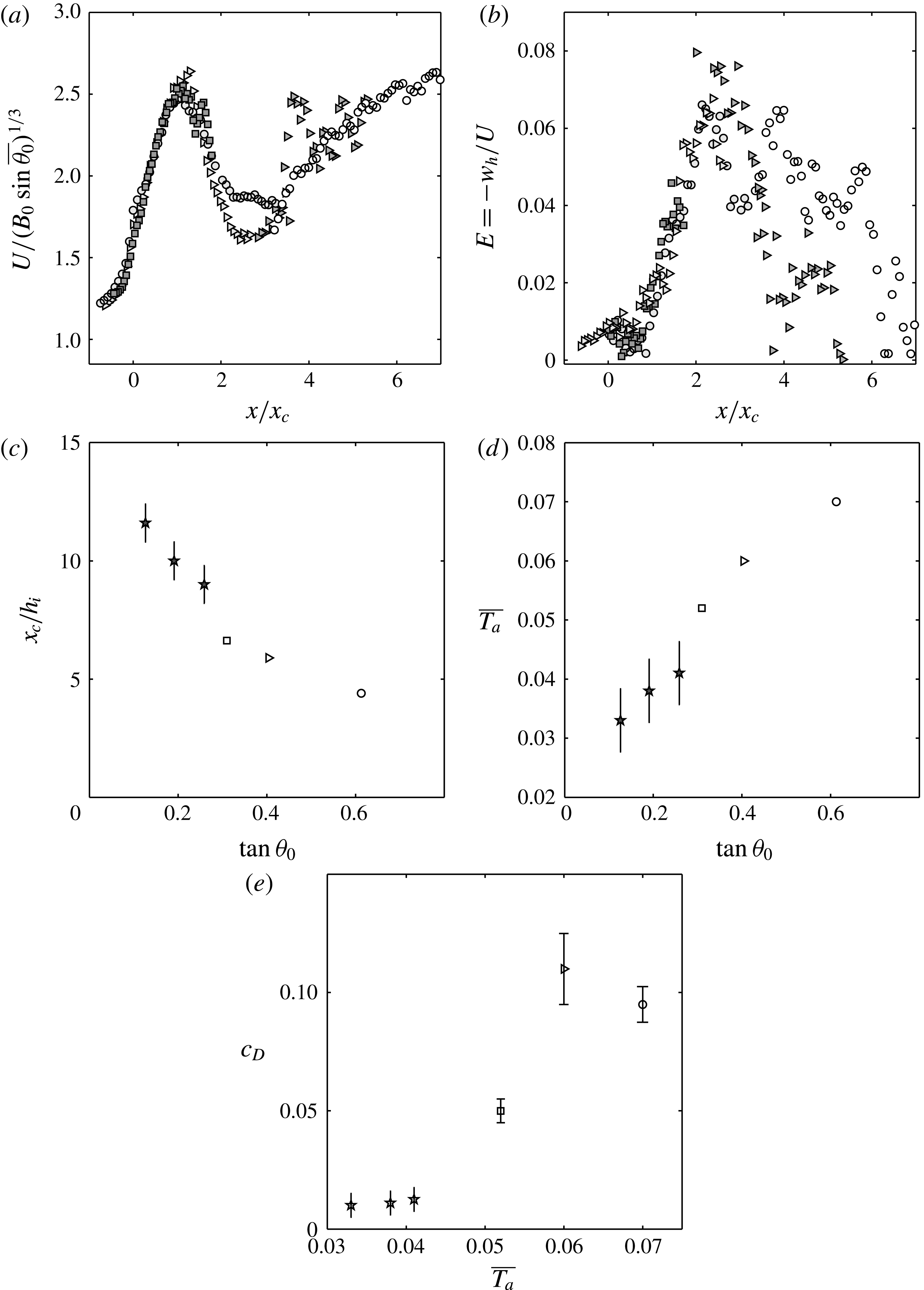
In figure 10(a), the depth-integrated velocities are plotted for all experiments using
 $x_{c}\equiv x_{c,exp}$
to normalize the downstream direction
 $x$
and using
 $(B_{0}\sin \overline{\unicode[STIX]{x1D703}})^{1/3}$
to normalize the velocity
 $U$
. We see that the velocity data nicely collapse onto a single curve
 $x/x_{c}\leqslant 1$
, with a non-dimensional velocity maximum of approximately
 $2.6$
. Different decays are observed for
 $x>x_{c}$
for the different experiments, including experiment C1, for which a near overlap between the equilibrium-state velocity and the experimental velocity has been highlighted in § 5 (cf. figure 5
a) close to the end of the slope, where bottom drag starts to be dominant. The first velocity minimum is at
 $x/x_{c}\approx 2.5$
for all experiments.
(a) Depth-integrated velocity normalized by
 $(B_{0}\sin \overline{\unicode[STIX]{x1D703}})^{1/3}$
, (b) entrainment rates
 $E=-w_{h}/U$
along
 $x$
normalized by
 $x_{c}\equiv x_{c,exp}$
for all experiments, (c) the ratio
 $x_{c}/h_{i}$
, (d)
 $\overline{T_{a}}$
versus the slope
 $\tan \unicode[STIX]{x1D703}$
and (e) estimated bottom drag coefficients
 $c_{D}$
versus
 $\overline{T_{a}}$
; ▫, experiment C1; ○, C3; ▹, L2;
 $\star$
, from Pawlak & Armi (Reference Pawlak and Armi2000) with
 $\unicode[STIX]{x1D703}=14.5^{\circ },10.8^{\circ },7.2^{\circ }$
.

Using the same scale to non-dimensionalize the downstream direction, we also plot the entrainment rates
 $E=-w_{h}/U$
for all experiments in figure 10(b) and we see that the values collapse onto a curve for
 $x<2.5x_{c}$
, while there is a spread when
 $x>2.5x_{c}$
. The maximal values are obtained for experiments C3 and L2, with an abrupt slope change at the ridge with
 $E_{max}\approx 0.07{-}0.08$
.
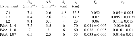
Summary of the key parameters for the present experiments and those of Pawlak & Armi (Reference Pawlak and Armi2000) with
 $\unicode[STIX]{x1D703}=14.5^{\circ }$
(L14),
 $10.8^{\circ }$
(L10) and
 $7.2^{\circ }$
(L07).
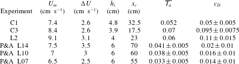
It is clear that a smooth transition to an equilibrium flow governed by (2.11) requires that the initial acceleration of the current, expressed by an acceleration parameter, remains below a certain value. The local value of
 $T_{a}$
, as shown in figures 5(e) and 6(e), is not appropriate because it depends on the local flow parameters. We can introduce an overall acceleration parameter in the form
 $$\begin{eqnarray}\overline{T_{a}}=\frac{h_{i}}{U_{m}}\frac{\unicode[STIX]{x0394}U}{x_{c}},\end{eqnarray}$$
where
 $x_{c}$
is the position of maximum velocity
 $U_{m}$
,
 $\unicode[STIX]{x0394}U=U_{m}-U_{i}$
and
 $h_{i}$
is the initial current height. All values are summarized in table 2, giving
 $\overline{T_{a}}=0.052$
for experiment C1,
 $\overline{T_{a}}=0.07$
for experiment C3 and
 $\overline{T_{a}}=0.06$
for experiment L2. These values are close to the local
 $T_{a}$
(figure 6(e) for experiment C3) at midposition,
 $x=x_{c}/2$
. An alternative and quantitative estimation of the overall acceleration parameter can be made using the definition of
 $Ri$
, from which we get
 $U_{i}=(B\cos \unicode[STIX]{x1D703}_{i}/Ri_{i})^{1/3}$
and
 $U_{m}=(B\cos \unicode[STIX]{x1D703}_{m}/Ri_{c})^{1/3}$
. This gives
 $$\begin{eqnarray}\unicode[STIX]{x0394}U/U_{m}=1-\left(\frac{Ri_{c}\cos \unicode[STIX]{x1D703}_{i}}{Ri_{i}\cos \unicode[STIX]{x1D703}_{c}}\right)^{1/3},\quad \text{and hence}\quad \frac{x_{c}}{h_{i}}={\displaystyle \frac{1-\left(\displaystyle \frac{Ri_{c}\cos \unicode[STIX]{x1D703}_{i}}{Ri_{i}\cos \unicode[STIX]{x1D703}_{c}}\right)^{1/3}}{\overline{T}_{a}}}.\end{eqnarray}$$
From figures 5(b), 6(b) and 9(b), the critical bulk Richardson number is taken as
 $Ri_{c}\approx 0.13$
and
 $Ri_{i}\approx 0.45$
at
 $x=0$
. Pawlak & Armi (Reference Pawlak and Armi2000) obtain a value of
 $J_{c}\sim 0.2$
in their experiments defined with
 $\unicode[STIX]{x1D6FF}_{I\unicode[STIX]{x1D708}}$
and maximum velocity. We take here for their experiments
 $Ri_{c}=0.15$
and
 $Ri_{i}=0.65$
. With these values, we get for the present experiments
 $\unicode[STIX]{x0394}U/U_{m}\sim 0.35$
, which is very close to the values obtained by taking the velocity measurements directly; for their experiments,
 $\unicode[STIX]{x0394}U/U_{m}\sim 0.37$
. It seems thus that this ratio varies very little (10 % maximum) depending on the initial acceleration.
In figure 10(c), we plot
 $x_{c}/h_{i}$
as a function of the initial slope
 $\tan \unicode[STIX]{x1D703}_{0}$
, including also the results of Pawlak & Armi (Reference Pawlak and Armi2000) (
 $\star$
), with errorbars coming from the uncertainty in estimating the values of
 $x_{c}$
,
 $h_{i}$
,
 $\unicode[STIX]{x0394}U$
and
 $U_{m}$
from their plots. In figure 6, it is seen that in the present experiments
 $\overline{T}_{a}\sim 0.07$
for the conditions of experiment C3 and decreases to
 $\overline{T}_{a}\sim 0.052$
in C1 (cf. figure 5). In the latter, a weak oscillation would be observed if the slope did not decrease rapidly to zero beyond the maximum velocity. Figure 10(d) plots
 $\overline{T_{a}}$
as a function of the slope, making
 $x_{c}/h_{i}$
independent of the initial conditions of the flow
 $\unicode[STIX]{x0394}U/U_{m}$
. We see in both plots 10(c) and (d) that, in general, as the slope increases, the acceleration is larger and the position in which the Richardson number becomes critical and the maximal velocity is reached decreases. The data of Pawlak & Armi (Reference Pawlak and Armi2000) are shifted upwards and are higher for the same slope because the interface is unstable from the start, which adds additional drag via entrainment, thus reducing the acceleration. When the slope angle decreases and approaches zero, the distance required to reach the equilibrium-state velocity will tend to be very large, as we can extract from figure 10(c). We can conclude that a gradual acceleration up to maximum velocity without oscillations requires that
 $\overline{T}_{a}<0.05$
, as in the experiments of Pawlak & Armi (Reference Pawlak and Armi2000) and marginally for our experiment C1.
Finally, we plot the bottom drag coefficients
 $c_{D}$
as a function of the overall acceleration parameter
 $\overline{T_{a}}$
in figure 10(e). We see that for small acceleration parameters
 $\overline{T_{a}}<0.05$
, as in the experiments of Pawlak & Armi (Reference Pawlak and Armi2000), values remain low. As
 $\overline{T_{a}}$
approaches the value of
 $0.05$
,
 $c_{D}$
increases rapidly to reach a much larger value. For the experiments of Pawlak & Armi (Reference Pawlak and Armi2000), the values of
 $c_{D}$
have been evaluated using (2.9), taking
 $E=0.02$
and taking the local acceleration parameter
 $\overline{T_{a}}=0$
at maximum velocity. This gives
 $c_{D}<0.02$
. Errorbars are relative to the uncertainty in evaluating their final entrainment
 $E$
, velocity
 $U$
and current depth
 $h_{0}$
.
8 Conclusions
Our results show that the interface thickness and shear across the interface at the start of the slope are crucial for the nature of the gravity current downhill. They determine, together with the acceleration down the slope, the flow instability and the size of the KH billows, and therewith the flow evolution. We can summarize the main results that emerge from the present study as follows.
-
(i) When a gravity current with an initially thick and stable interface (high
 $J$
) on a horizontal or nearly horizontal boundary moves onto a steep slope, it is first stable (zone I), and then, as a consequence of shear instabilities of the interface and KH billows (zone II), undergoes a cycle of accelerations and decelerations and does not reach the constant equilibrium velocity within the distance
$x_{c}$
of approximately
$30h_{0}$
considered. Subsequently, it evolves towards a state of collapsed KH billows on top of the accelerating dense gravity current (zone III). As mentioned in the introduction, this evolution is quite different from the flow over a weir, accelerating on a slope, as investigated by Pawlak & Armi (Reference Pawlak and Armi2000), where the current has from the beginning a thin unstable interface. At the start of the slope where the interfacial Richardson number
$J$
is below critical, the KH billows are small and a typical stratified shear layer develops on top of the gravity current. As a consequence, the current accelerates smoothly to reach a nearly constant velocity at a distance
$x_{c}$
of the order of
$10h_{0}$
, the distance
$x_{c}$
increasing with decreasing slope. Depending on the value of an overall acceleration parameter, defined within this paper, the flow may approach or not this quasiequilibrium between gravity and total drag (bottom and interfacial); a transition value is evaluated to be
$\overline{T_{a}}=0.05$
. The distance
$x_{c}$
to reach the first velocity maximum, corresponding also to the onset of KH instabilities, normalized by the initial current depth, decreases as the initial slope rises. A remarkable observation is that the head velocity accelerates smoothly and is not or is little affected by the velocity variation of the layer behind. The value of the Richardson number at the sill (
$x=0$
), and in particular the shear thickness
$\unicode[STIX]{x1D6FF}_{I\unicode[STIX]{x1D708}}$
, are thus important for the flow nature and existence of zone I. Further downslope, the value of
$\unicode[STIX]{x1D6FF}_{I\unicode[STIX]{x1D708}}$
does not vary much, and variations in
$u_{m}^{2}$
due to accelerations are more relevant. Therefore, to characterize the flow, the acceleration parameter
$T_{a}$
discussed in § 7 is used. This parameter is also relatively easy to measure from experimental data.
-
(ii) The first KH billows cause boundary layer separation and reattachment, which lead to a large boundary friction coefficient which is of the order of the interfacial drag due to entrainment. The high values of
$c_{D}$
obtained from velocity data are consistent with the observed values of the Reynolds stresses in the boundary layer, reaching values of
$\overline{u^{\prime }w^{\prime }}/u_{m}^{2}$
of
$5\,\%{-}8\,\%$
. Dye visualizations have shown the continuous formation of billows (1 cm) in the bottom boundary layer coupled with the development of the large KH billows at the interface (figure 8). The small billows in the boundary layer are characteristic of boundary layer separation. -
(iii) The spatial development on a concave boundary, more representative of natural slopes, is very similar to that on a constant slope boundary, so that it is rather the sudden slope change that causes the observed different behaviour in the development of the gravity flow with respect to previously studied constant velocity gravity flows on a slope. Possible centrifugal instabilities due to boundary curvature do not change the dynamics. Brun (Reference Brun2017) performed numerical simulation of katabatic winds down a slope with a hyperbolic tangent shape (first convex then concave) using the mesoscale model MesoNH code developed at Météo France, coupled to a three-dimensional large-eddy simulation parametrization. He reported the formation of Görtler instabilities in the outer part of the velocity profile (at the interface and above) where the density stratification is weak, which modify vertical mixing and the vertical turbulent transport. Albayrak, Hopfinger & Lemmin (Reference Albayrak, Hopfinger and Lemmin2008) studied a wall jet on a concave boundary and reported significant changes in the boundary layer characteristics when Görtler instabilities were present. We performed cross-stream slit lighting and dye injections at the boundary but could not detect any Görtler vortices near the boundary for the parameter range investigated. Up to onset of KH instability, the boundary layer has a low
$c_{D}$
and Görtler vortices if present would only increase
$c_{D}$
by less than a factor of 4 (Swearingen & Blackwelder Reference Swearingen and Blackwelder1987).


An open question concerns the role played by the ratio
 $\unicode[STIX]{x1D6FF}_{Bv}/\unicode[STIX]{x1D6FF}_{Iv}\sim 0.1$
between the thickness of the lower layer of the current and the interface thickness, which is quite small in the present experiments. The presence of acceleration–deceleration cycles and the overshoot may not only be a consequence of the sudden slope change, but could also depend on this ratio: for a deep density current for which the ratio is of order one, bottom friction may not slow down the flow and cause the overshoot as in the present experiments and the current may accelerate until it reaches a constant velocity, as predicted for the equilibrium state. In our case, KH billows can grow such that the vorticity regions approach the lower boundary layer, creating thus locally high velocity gradients and thus bottom friction coefficients, causing subsequently the strong deceleration.
Acknowledgements
This work has been supported by a grant from Labex OSUG
 $@2020$
(Investissements d’avenir ANR10 LABX56). We are grateful to M. Ungarish for helpful discussions. Special thanks go to J.-M. Barnoud, S. Mercier and S. Viboud for their precious technical support.