1 Introduction
Encapsulated bubbles are used widely in the application of ultrasound contrast-enhanced agents (Lindner Reference Lindner2004) and drug-carrier capsules (Unger et al. Reference Unger, Hersh, Vannan, Matsunaga and Mccreery2001). Interaction with surrounding bubbles affects their behaviour, leading to phenomena such as erratic drift (Strasberg & Benjamin Reference Strasberg and Benjamin1958), bubble grapes (Kobelev, Ostrovskii & Sutin Reference Kobelev, Ostrovskii and Sutin1979), acoustic streaming (Akhatov, Parlitz & Lauterborn Reference Akhatov, Parlitz and Lauterborn1994), and multibubble sonoluminescence (Crum Reference Crum1994). A study on the interaction of two bubbles may shed light on the dynamics of bubble groups, which is the motivation of this work.
The dynamics of two gas bubbles without encapsulating membranes has been extensively investigated, which goes back to the pioneering work by Bjerknes (Reference Bjerknes1906). The well-known Bjerknes force is the radiation force generated by the applied sound field (primary Bjerknes force) or by the oscillation of a nearby bubble (secondary Bjerknes force). We focus on the secondary Bjerknes force in this paper. Bjerknes’ theory states that the two bubbles attract each other when they oscillate in phase (
 $\unicode[STIX]{x0394}\unicode[STIX]{x1D719}<\unicode[STIX]{x03C0}/2$
or
 $\unicode[STIX]{x0394}\unicode[STIX]{x1D719}>3\unicode[STIX]{x03C0}/2$
), and repel each other when out of phase (
 $\unicode[STIX]{x03C0}/2<\unicode[STIX]{x0394}\unicode[STIX]{x1D719}<3\unicode[STIX]{x03C0}/2$
), where
 $\unicode[STIX]{x0394}\unicode[STIX]{x1D719}$
is the phase difference. This theory is based on the balance between the inertia of the added mass and the secondary Bjerknes force:
 $$\begin{eqnarray}\frac{\text{d}}{\text{d}t}\left(\frac{1}{2}\unicode[STIX]{x1D70C}V_{bi}v_{i}\right)=-2\unicode[STIX]{x03C0}\unicode[STIX]{x1D70C}\frac{R_{i}^{2}}{L^{2}}\frac{\text{d}}{\text{d}t}(R_{i}R_{j}^{2}{\dot{R}}_{j}),\end{eqnarray}$$
where
 $\unicode[STIX]{x1D70C}$
is the density of the surrounding liquid,
 $V_{b}$
the bubble volume,
 $v$
the translational velocity and
 $R$
the bubble radius, with subscripts
 $i$
and
 $j$
denoting the two bubbles, respectively, and
 $L$
is the distance between the two bubbles. The right-hand side of (1.1) is the Bjerknes force, denoted by
 $F_{B}$
in the following. Assuming the radial oscillation as
 $R_{i}(t)=R_{0i}[1+\unicode[STIX]{x1D6FF}_{i}\cos (\unicode[STIX]{x1D714}_{d}t+\unicode[STIX]{x1D719}_{i})]$
, where
 $R_{0}$
is the equilibrium radius,
 $\unicode[STIX]{x1D6FF}$
,
 $\unicode[STIX]{x1D714}_{d}$
and
 $\unicode[STIX]{x1D719}$
are the amplitude, frequency and phase angle of the oscillation, respectively, and averaging the Bjerknes force over one oscillatory cycle, one obtains:
 $$\begin{eqnarray}\displaystyle \langle F_{B}\rangle & = & \displaystyle -\frac{\unicode[STIX]{x1D714}_{d}}{2\unicode[STIX]{x03C0}}\int _{0}^{2\unicode[STIX]{x03C0}/\unicode[STIX]{x1D714}_{d}}2\unicode[STIX]{x03C0}\unicode[STIX]{x1D70C}\frac{R_{i}^{2}}{L^{2}}\frac{\text{d}}{\text{d}t}(R_{i}R_{j}^{2}{\dot{R}}_{j})\,\text{d}t\nonumber\\ \displaystyle & = & \displaystyle \frac{\unicode[STIX]{x03C0}\unicode[STIX]{x1D70C}\unicode[STIX]{x1D714}_{d}^{2}R_{0i}^{3}R_{0j}^{3}}{4L^{2}}\unicode[STIX]{x1D6FF}_{i}\unicode[STIX]{x1D6FF}_{j} [\!8\cos \unicode[STIX]{x0394}\unicode[STIX]{x1D719}+8\unicode[STIX]{x1D6FF}_{i}\unicode[STIX]{x1D6FF}_{j}\cos 2\unicode[STIX]{x0394}\unicode[STIX]{x1D719}\nonumber\\ \displaystyle & & \displaystyle +\,2(\unicode[STIX]{x1D6FF}_{i}^{2}+\unicode[STIX]{x1D6FF}_{j}^{2})\cos \unicode[STIX]{x0394}\unicode[STIX]{x1D719}+\unicode[STIX]{x1D6FF}_{i}^{2}\unicode[STIX]{x1D6FF}_{j}^{2}\cos \unicode[STIX]{x0394}\unicode[STIX]{x1D719}\cos 2\unicode[STIX]{x0394}\unicode[STIX]{x1D719}\!],\end{eqnarray}$$
where
 $\unicode[STIX]{x0394}\unicode[STIX]{x1D719}=\unicode[STIX]{x1D719}_{i}-\unicode[STIX]{x1D719}_{j}$
. Neglecting the final three terms in the bracket under the assumption that
 $\unicode[STIX]{x1D6FF}_{i},\unicode[STIX]{x1D6FF}_{j}\ll 1$
, (1.2) reduces to
 $$\begin{eqnarray}\displaystyle \langle F_{B}\rangle =\frac{2\unicode[STIX]{x03C0}\unicode[STIX]{x1D70C}\unicode[STIX]{x1D714}_{d}^{2}R_{01}^{3}R_{02}^{3}}{L^{2}}\unicode[STIX]{x1D6FF}_{1}\unicode[STIX]{x1D6FF}_{2}\cos \unicode[STIX]{x0394}\unicode[STIX]{x1D719}, & & \displaystyle\end{eqnarray}$$
which is consistent with that derived by Crum (Reference Crum1975). It is clear that
 $\langle F_{B}\rangle >0$
when
 $\unicode[STIX]{x0394}\unicode[STIX]{x1D719}<\unicode[STIX]{x03C0}/2$
or
 $\unicode[STIX]{x0394}\unicode[STIX]{x1D719}>3\unicode[STIX]{x03C0}/2$
, indicating an attractive force; and
 $\langle F_{Bi}\rangle <0$
when
 $\unicode[STIX]{x03C0}/2<\unicode[STIX]{x0394}\unicode[STIX]{x1D719}<3\unicode[STIX]{x03C0}/2$
, indicating a repulsive force.
The classical Bjerknes theory reviewed above is only applicable to spherical gas bubbles under harmonic oscillations with small oscillatory amplitudes and without the effects of viscosity and higher-order terms. The translational direction may reverse when bubbles oscillate in an ultraharmonics mode (Oguz & Prosperetti Reference Oguz and Prosperetti1990), or a strong driving force is applied (Doinikov Reference Doinikov2001), or viscous effects become significant (Doinikov Reference Doinikov1999, Reference Doinikov2002), or the higher-order terms in (1.2) are considered (Barbat, Ashgriz & Liu Reference Barbat, Ashgriz and Liu1999; Ida Reference Ida2003). In addition, Bjerknes’ theory states that bubbles repel when the driving frequency is between their natural frequencies, or attract when beyond their natural frequencies. On the other hand, Zabolotskaya (Reference Zabolotskaya1984) and Doinikov & Zavtrak (Reference Doinikov and Zavtrak1995) found that the natural frequencies increase when the two bubbles come closer, which leads to a sign reversal in the Bjerknes force. In addition to repulsive or attractive motion, the bubble pair may undergo stable translational oscillation (Barbat et al. Reference Barbat, Ashgriz and Liu1999; Harkin, Kaper & Nadim Reference Harkin, Kaper and Nadim2001) and acoustic streaming (Pelekasis et al. Reference Pelekasis, Gaki, Doinikov and Tsamopoulos2004), contrary to Bjerknes’ theory. Bjerknes’ theory provides a fundamental perspective on the mutual force of a pair of gas bubbles. Nevertheless, additional effects in practical situations contribute to the behaviour of the two bubbles and need to be investigated. In this paper, we emphasize the influences of encapsulating membranes and shape oscillation.
In many situations, shape oscillations can cause translational motion of a bubble. The erratic drift of a bubble in a sound field has been shown to be the result of the resonance of a shape mode with the breathing mode both experimentally (Eller & Crum Reference Eller and Crum1970) and theoretically (Benjamin & Ellis Reference Benjamin and Ellis1990; Mei & Zhou Reference Mei and Zhou1991). Bjerknes’ theory does not consider the effects of deformation, implying the separation distance between the bubbles should be large compared to the bubble sizes. When the bubbles are close to each other, the shape modes are no longer negligible. The dynamic equations of two non-spherical gas bubbles were derived in Takahira, Akamatsu & Fujikawa (Reference Takahira, Akamatsu and Fujikawa1991), which predicts that instability can occur on the far sides of the two bubbles. Chahine & Duraiswami (Reference Chahine and Duraiswami1992) investigated the dynamics of a multibubble cloud using a boundary element method (BEM) based on potential theory. Bui et al. (Reference Bui, Ong, Khoo, Klaseboer and Hung2006) developed a fast BEM algorithm to simulate the multibubble dynamics. Hejazialhosseini, Rossinelli & Koumoutsakos (Reference Hejazialhosseini, Rossinelli and Koumoutsakos2013) presented a volume-rendering technique to visualize the bubble–shock interactions. Significant shape oscillations in response to a step variation in pressure (Pelekasis & Tsamopoulos Reference Pelekasis and Tsamopoulos1993a ; Chatzidai, Dimakopoulos & Tsamopoulos Reference Chatzidai, Dimakopoulos and Tsamopoulos2011) or an oscillatory pressure field (Pelekasis & Tsamopoulos Reference Pelekasis and Tsamopoulos1993b ) were demonstrated in an inviscid (Pelekasis & Tsamopoulos Reference Pelekasis and Tsamopoulos1993a ,Reference Pelekasis and Tsamopoulos b ) or a viscous (Chatzidai et al. Reference Chatzidai, Dimakopoulos and Tsamopoulos2011) fluid. The classical Bjerknes force might be revised with regard to the deformation. The expression of mutual force, with contributions from the amplitude of shape modes, was derived and is applicable to a linear oscillation (Doinikov & Zavtrak Reference Doinikov and Zavtrak1995).
When bubbles are encapsulated in membranes, their behaviour is different from that of gas bubbles, due to the generation of additional stresses and different interfacial conditions. One of the reasons for the different behaviour is the shift of natural frequencies due to the presence of the membrane (Liu et al.
Reference Liu, Sugiyama, Takagi and Matsumoto2011; Tsiglifis & Pelekasis Reference Tsiglifis and Pelekasis2011), leading to different conditions for interfacial instability. Besides, the interface between the liquid and membrane is subject to a no-velocity-jump condition, because the liquid particles adhere to the membrane, unlike a gas bubble whose interface is free of shear stresses, or free-slip. The material points on the membrane move along the surface under tension, which supports the stress balance in the tangential direction and retards the surrounding flow. For a gas bubble, vorticity is confined to the vicinity of the surface if the viscosity is not too large, or more rigorously, if the viscous penetration depth is much smaller than the bubble radius, so that the viscous force can be predicted based on a potential flow. When the viscosity is not small, however, the diffusion of vorticity from the interface into the flow field is not negligible and renders an opposite translation of the bubble (Doinikov Reference Doinikov2002). The no-velocity-jump interface, moreover, excludes the neglecting the effect of the vorticity distribution on the fluid (Doinikov Reference Doinikov1999), as in the case of encapsulated bubble (Liu et al.
Reference Liu, Sugiyama, Takagi and Matsumoto2012). The drag of a gas bubble or a rigid sphere translating in a fluid has been studied thoroughly. The drag coefficient
 $48/Re$
(where
 $Re$
is the Reynold’s number) is acknowledged for a spherical gas bubble with a free-slip interface (Levich Reference Levich1949; Kang & Leal Reference Kang and Leal1988), or
 $24/Re$
for a rigid sphere with a no-slip interface (Batchelor Reference Batchelor1967). The no-velocity-jump condition on an elastic membrane is expected to be in the intermediate range between free-slip and no-slip conditions.
The studies on the encapsulated bubble reviewed above mainly focus on a single bubble. The extension of the dynamics of a single bubble to those of two bubbles is not trivial. The coupling of the translation and shape modes makes the mathematical derivation cumbersome. In this paper, we establish a theoretical model of two interacting encapsulated bubbles under nonlinear radial motion and linear shape oscillations. To include vorticity distribution, we use Prosperetti’s model (Prosperetti Reference Prosperetti1977) and solve the potential flow with a viscous correction. The membrane stress is coupled based on the theory of elastic membranes by Green & Adkins (Reference Green and Adkins1960), which has been applied to studies on the capsule–fluid interaction (Barthès-Biesel & Rallison Reference Barthès-Biesel and Rallison1981; Barthès-Biesel & Sgaier Reference Barthès-Biesel and Sgaier1985; Li, Barthès-Biesel & Helmy Reference Li, Barthès-Biesel and Helmy1988; Leyrat-Maurin & Barthès-Biesel Reference Leyrat-Maurin and Barthès-Biesel1994; Quéguiner & Barthès-Biesel Reference Quéguiner and Barthès-Biesel1997; Diaz, Pelekasis & Barthès-Biesel Reference Diaz, Pelekasis and Barthès-Biesel2000; Lac et al. Reference Lac, Barthès-Biesel, Pelekasis and Tsamopoulos2004; Pozrikidis Reference Pozrikidis2001, Reference Pozrikidis2003a ,Reference Pozrikidis b , Reference Pozrikidis2005).
The rest of the paper is organized as follows. In § 2, we present the mathematical formulation. The potential flow field, the viscous correction, and the membrane mechanics will be derived, respectively. The governing equations are summarized in § 2.6. In § 3.1, we compare our results with the experimental measurements obtained by Garbin et al. (Reference Garbin, Dollet, Overvelde, Cojoc, Di Fabrizio, Van Wijngaarden, Prosperetti, De Jong, Lohse and Versluis2009) to investigate the membrane effects. In § 3.2, the potential flow model is validated by comparing its results with the experimental observations by Lauterborn & Bolle (Reference Lauterborn and Bolle1975). The effects of driving frequency and phase difference on the behaviour of two gas or encapsulated bubbles are revealed in § 3.3. The contributions of different forces are compared in § 3.4. Concluding remarks are given in § 4.
2 Problem formulation
2.1 General formulation
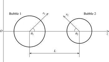
In this section, we derive the mathematical formulation for the dynamics of two bubbles suspended in an unbounded fluid. We establish an axisymmetric coordinate system with the symmetric axis
 $Oz$
connecting the centres of the two bubbles, as shown in figure 1. In this coordinate system, the bubbles translate along
 $Oz$
. The distance of separation between the two centres is denoted by
 $L$
. The radial motions and deformations of the bubbles are described by the local polar coordinates (
 $r_{1},\unicode[STIX]{x1D703}_{1}$
) or (
 $r_{2},\unicode[STIX]{x1D703}_{2}$
). In the following equations, the subscript
 $i$
denotes the one bubble, and
 $j=3-i$
denotes the other one. Only the equations for bubble
 $i$
are written, and the equations for bubble
 $j$
are equivalent, with
 $i$
and
 $j$
exchanged.
The coordinate system of two bubbles.

The velocity
 $\boldsymbol{u}$
and pressure
 $p$
of the external field are governed by the incompressible Navier–Stokes equations:
 $$\begin{eqnarray}\displaystyle & \displaystyle \unicode[STIX]{x1D735}_{i}\boldsymbol{\cdot }\boldsymbol{u}=0, & \displaystyle\end{eqnarray}$$
 $$\begin{eqnarray}\displaystyle & \displaystyle \unicode[STIX]{x1D70C}\frac{\unicode[STIX]{x2202}\boldsymbol{u}}{\unicode[STIX]{x2202}t}+\unicode[STIX]{x1D70C}[(\boldsymbol{u}-v_{i}\boldsymbol{e}_{z})\boldsymbol{\cdot }\unicode[STIX]{x1D735}_{i}]\boldsymbol{u}=-\unicode[STIX]{x1D735}_{i}p+\unicode[STIX]{x1D707}_{l}\unicode[STIX]{x1D735}_{i}\boldsymbol{\cdot }(\unicode[STIX]{x1D735}_{i}\boldsymbol{u}+\unicode[STIX]{x1D735}_{i}\boldsymbol{u}^{\text{T}}), & \displaystyle\end{eqnarray}$$
where
 $\unicode[STIX]{x1D70C}$
and
 $\unicode[STIX]{x1D707}_{l}$
are the liquid density and viscosity, respectively.
 $\unicode[STIX]{x1D735}_{i}$
denotes the gradient, of which the origin is attached to the centroid of the bubble
 $i$
.
 $v_{i}$
is the translational velocity of bubble
 $i$
in the direction along
 $Oz$
. We neglect the flow field within the bubbles due to the negligible density and viscosity of gas. The internal pressure
 $p_{gi}$
is assumed to be spatially uniform and varies in time according to the polytropic process:
 $$\begin{eqnarray}p_{gi}=p_{g0i}\left(\frac{V_{0bi}}{V_{bi}}\right)^{\unicode[STIX]{x1D6E4}},\end{eqnarray}$$
where
 $V_{bi}$
is the volume of bubble
 $i$
, and the subscript 0 indicates the initial value.
 $\unicode[STIX]{x1D6E4}$
is the polytropic index.
In the presence of the encapsulating membrane, the bubble interface
 $S_{i}$
is subjected to a no-velocity-jump condition, yielding continuities of the velocities in both the normal and tangential directions:
 $$\begin{eqnarray}\boldsymbol{u}_{mi}=\boldsymbol{u}_{li}\quad \text{on}~S_{i},\end{eqnarray}$$
where the subscripts
 $m$
and
 $l$
represent the material points on the membrane and in the liquid, respectively. The continuity of velocity in the normal direction yields the kinematic boundary condition:
 $$\begin{eqnarray}\frac{\unicode[STIX]{x2202}S_{i}}{\unicode[STIX]{x2202}t}+(\boldsymbol{u}-v_{i}\boldsymbol{e}_{z})\boldsymbol{\cdot }\unicode[STIX]{x1D735}_{i}S_{i}=0.\end{eqnarray}$$
The dynamic boundary condition provides the balance of the pressure difference across the interface, the viscous stress of the fluid, and the membrane stress, i.e.
 $$\begin{eqnarray}\boldsymbol{n}_{i}\boldsymbol{\cdot }(-p\unicode[STIX]{x1D644}_{i}+2\unicode[STIX]{x1D707}_{l}\unicode[STIX]{x1D640}_{i})=\boldsymbol{n}_{i}\boldsymbol{\cdot }(-p_{gi}\unicode[STIX]{x1D644}_{i})+(\unicode[STIX]{x1D6FE}\unicode[STIX]{x1D735}_{i}\boldsymbol{\cdot }\boldsymbol{n}_{i})\boldsymbol{n}_{i}+\boldsymbol{F}_{i}\quad \text{on}~S_{i},\end{eqnarray}$$
where
 $\unicode[STIX]{x1D644}_{i}$
and
 $\boldsymbol{n}_{i}$
are the unit tensor and unit normal vector with respect to the local polar coordinate,
 $\unicode[STIX]{x1D640}_{i}=(\unicode[STIX]{x1D735}_{i}\boldsymbol{u}+\unicode[STIX]{x1D735}_{i}\boldsymbol{u}^{\text{T}})/2$
the strain rate tensor, and
 $\boldsymbol{F}_{i}$
the membrane stress. The surface tension with coefficient
 $\unicode[STIX]{x1D6FE}$
is included here so that our model can be used for gas bubbles when membrane stress is set to be zero. For encapsulated bubbles, the surface tension is set to be zero. At infinity, we assume that
 $$\begin{eqnarray}\boldsymbol{u}\rightarrow 0,\quad p\rightarrow p_{\infty }~\text{at infinity}.\end{eqnarray}$$
We decompose velocity and pressure into the potential (with subscript
 $p$
) and the viscous correction (with subscript
 $v$
) parts:
 $$\begin{eqnarray}\boldsymbol{u}=\boldsymbol{u}_{p}+\boldsymbol{u}_{v},\quad p=p_{p}+p_{v}.\end{eqnarray}$$
We will discuss the solution procedures for these two parts in detail in the later sections.
2.2 Geometry of the bubble
We assume that the dominant motion is in the radial direction with perturbations due to translational motion and deformations. The perturbation to a spherical bubble can be expanded in terms of the spherical harmonics. Since we consider the axisymmetric model for simplicity in this paper, the spherical harmonics reduces to the Legendre polynomials, as the azimuthal mode is constant. For a gas bubble, the normal stress jump across the interface due to the surface tension is a function of the curvature, computed using the normal component of the interfacial displacement. By contrast, for an encapsulated bubble, the in-plane stress occurs as a resistance to the tangential displacement of the membrane. Therefore, in the present study, the tangential displacement must be computed, and is written using the associated Legendre polynomial
 $P_{k}^{1}(\cos \unicode[STIX]{x1D703}_{i})(=\text{d}P_{k}(\cos \unicode[STIX]{x1D703}_{i})/\text{d}\unicode[STIX]{x1D703}_{i})$
. The position of the material point on the membrane is therefrom expressed in radial and zenith directions:
 $$\begin{eqnarray}\displaystyle r_{i}(\unicode[STIX]{x1D703}_{i},t) & = & \displaystyle R_{i}(t)+\mathop{\sum }_{k=2}^{\infty }a_{ki}(t)P_{k}(\cos \unicode[STIX]{x1D703}_{i}),\quad a_{ki}\ll R_{i},\end{eqnarray}$$
 $$\begin{eqnarray}\displaystyle \unicode[STIX]{x1D6E9}_{i}(\unicode[STIX]{x1D703}_{i},t) & = & \displaystyle \unicode[STIX]{x1D703}_{i}+\frac{1}{R_{i}(t)}\mathop{\sum }_{k=1}^{\infty }b_{ki}(t)P_{k}^{1}(\cos \unicode[STIX]{x1D703}_{i}),\quad b_{ki}/R_{i}\ll \unicode[STIX]{x1D703}_{i}.\end{eqnarray}$$
The series of Legendre polynomials
 $P_{k}(\cos \unicode[STIX]{x1D703}_{i})$
represents the perturbation in the radial direction with amplitudes of shape modes
 $a_{ki}$
. Notice
 $a_{1i}$
is the translational distance with the bubble shape unchanged and is related to the translational velocity
 $v_{i}$
, so that the summation in (2.9) is from
 $k=2$
. The series of associated Legendre polynomials
 $P_{k}^{1}(\cos \unicode[STIX]{x1D703}_{i})$
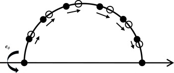
is the perturbation in the tangential direction due to deformation. For a special case, in which the volume and the shape are unchanged, as illustrated in figure 2,
 $b_{1i}P_{1}^{1}(\cos \unicode[STIX]{x1D703}_{i})$
denotes the extension or compression along the surface, inducing strain and thus stress in the membrane.
The movements of material points on the membrane at
 $b_{1i}P_{1}^{1}(\cos \unicode[STIX]{x1D703}_{i})$
.

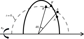
We assume an infinitesimal element
 $AB$
in the reference configuration is unstressed. As sketched in figure 3,
 $AB$
transforms to
 $A^{\prime }B^{\prime }$
after some time. According to the above definition of surface position, the coordinates of the material points
 $A$
,
 $B$
,
 $A^{\prime }$
and
 $B^{\prime }$
are
 $$\begin{eqnarray}A:[R_{0i},\unicode[STIX]{x1D703}_{i}],\quad \!A^{\prime }:[r_{i}(\unicode[STIX]{x1D703}_{i},t),\unicode[STIX]{x1D6E9}_{i}(\unicode[STIX]{x1D703}_{i},t)],\quad \!B:[R_{0i},\unicode[STIX]{x1D703}_{i}+\text{d}\unicode[STIX]{x1D703}_{i}],\quad \!B^{\prime }[r_{i}(\unicode[STIX]{x1D703}_{i}+\text{d}\unicode[STIX]{x1D703}_{i},t),\unicode[STIX]{x1D6E9}_{i}(\unicode[STIX]{x1D703}_{i}+\text{d}\unicode[STIX]{x1D703}_{i},t)],\end{eqnarray}$$
respectively. The arclength between
 $A$
and
 $B$
is
 $$\begin{eqnarray}\text{d}s_{i}^{R}=R_{0i}\,\text{d}\unicode[STIX]{x1D703}_{i},\end{eqnarray}$$
and the arclength between
 $A^{\prime }$
and
 $B^{\prime }$
is
 $$\begin{eqnarray}\displaystyle \text{d}s & = & \displaystyle \sqrt{[r_{i}(\unicode[STIX]{x1D703}_{i}+\text{d}\unicode[STIX]{x1D703}_{i},t)-r_{i}(\unicode[STIX]{x1D703}_{i},t)]^{2}+r_{i}^{2}[\unicode[STIX]{x1D6E9}_{i}(\unicode[STIX]{x1D703}_{i}+\text{d}\unicode[STIX]{x1D703}_{i},t)-\unicode[STIX]{x1D6E9}_{i}(\unicode[STIX]{x1D703}_{i},t)]^{2}}\nonumber\\ \displaystyle & = & \displaystyle \left[R_{i}+\mathop{\sum }_{k=2}^{\infty }a_{ki}(t)P_{k}(\cos \unicode[STIX]{x1D703}_{i})+\mathop{\sum }_{k=1}^{\infty }b_{ki}(t)\frac{\text{d}P_{k}^{1}(\cos \unicode[STIX]{x1D703}_{i})}{\text{d}\unicode[STIX]{x1D703}_{i}}\right]\text{d}\unicode[STIX]{x1D703}_{i}.\end{eqnarray}$$
Sketch of movements of material points.

The two principal strains
 $\unicode[STIX]{x1D706}_{\unicode[STIX]{x1D703}i}$
and
 $\unicode[STIX]{x1D706}_{\unicode[STIX]{x1D719}i}$
are defined by the extension ratio in the arclength direction and the change ratio of the distance from the axis of symmetry, respectively:
 $$\begin{eqnarray}\displaystyle & \displaystyle \unicode[STIX]{x1D706}_{\unicode[STIX]{x1D703}i}=\frac{\text{d}s_{i}}{\text{d}s_{i}^{R}}=\frac{R_{i}}{R_{0i}}+\mathop{\sum }_{k=2}^{\infty }\frac{a_{ki}}{R_{0i}}P_{k}(\cos \unicode[STIX]{x1D703}_{i})+\mathop{\sum }_{k=1}^{\infty }\frac{b_{ki}}{R_{0i}}\frac{\text{d}P_{k}^{1}(\cos \unicode[STIX]{x1D703}_{i})}{\text{d}\unicode[STIX]{x1D703}_{i}}, & \displaystyle\end{eqnarray}$$
 $$\begin{eqnarray}\displaystyle & \displaystyle \unicode[STIX]{x1D706}_{\unicode[STIX]{x1D719}i}=\frac{r_{i}\sin \unicode[STIX]{x1D6E9}_{i}}{R_{0i}\sin \unicode[STIX]{x1D703}_{i}}=\frac{R_{i}}{R_{0i}}+\mathop{\sum }_{k=2}^{\infty }\frac{a_{ki}}{R_{0i}}P_{k}(\cos \unicode[STIX]{x1D703}_{i})+\cot \unicode[STIX]{x1D703}_{i}\mathop{\sum }_{k=1}^{\infty }\frac{b_{ki}}{R_{0i}}P_{k}^{1}(\cos \unicode[STIX]{x1D703}_{i}). & \displaystyle\end{eqnarray}$$
On the other hand, the shape of the bubble is independent of the mode
 $b_{ki}P_{k}^{1}(\cos \unicode[STIX]{x1D703}_{i})$
. Therefore, we can define the surface function as
 $$\begin{eqnarray}S_{i}\equiv r_{i}-R_{i}-\mathop{\sum }_{k=2}^{\infty }a_{ki}P_{k}(\cos \unicode[STIX]{x1D703}_{i})=0.\end{eqnarray}$$
Other geometric quantities are subsequently obtained by the surface function (Liu et al.
Reference Liu, Sugiyama, Takagi and Matsumoto2012), including the unit normal vector
 $\boldsymbol{n}_{i}$
pointing into the fluid:
 $$\begin{eqnarray}\boldsymbol{n}_{i}=\frac{\unicode[STIX]{x1D735}_{i}S_{i}}{|\unicode[STIX]{x1D735}_{i}S_{i}|}\simeq \boldsymbol{e}_{ri}-\boldsymbol{e}_{\unicode[STIX]{x1D703}i}\mathop{\sum }_{k=2}^{\infty }\frac{a_{ki}}{R_{i}}P_{k}^{1}(\cos \unicode[STIX]{x1D703}_{i}),\end{eqnarray}$$
the tangential vector
 $\boldsymbol{t}_{i}$
:
 $$\begin{eqnarray}\boldsymbol{t}_{i}\simeq \boldsymbol{e}_{\unicode[STIX]{x1D703}i}+\boldsymbol{e}_{ri}\mathop{\sum }_{k=2}^{\infty }\frac{a_{ki}}{R_{i}}P_{k}^{1}(\cos \unicode[STIX]{x1D703}_{i}),\end{eqnarray}$$
and the two principal curvatures in the
 $\unicode[STIX]{x1D703}$
and
 $\unicode[STIX]{x1D719}$
directions:
 $$\begin{eqnarray}\displaystyle & \displaystyle \unicode[STIX]{x1D705}_{\unicode[STIX]{x1D703}i}=\frac{1}{R_{i}}-\mathop{\sum }_{k=2}^{\infty }\frac{a_{ki}}{R_{i}^{2}}\left(P_{k}(\cos \unicode[STIX]{x1D703}_{i})+\frac{\text{d}^{2}P_{k}(\cos \unicode[STIX]{x1D703}_{i})}{\text{d}\unicode[STIX]{x1D703}_{i}^{2}}\right), & \displaystyle\end{eqnarray}$$
 $$\begin{eqnarray}\displaystyle & \displaystyle \unicode[STIX]{x1D705}_{\unicode[STIX]{x1D719}i}=\frac{1}{R_{i}}-\mathop{\sum }_{k=2}^{\infty }\frac{a_{ki}}{R_{i}^{2}}(P_{k}(\cos \unicode[STIX]{x1D703}_{i})+\cot \unicode[STIX]{x1D703}_{i}P_{k}^{1}(\cos \unicode[STIX]{x1D703}_{i})). & \displaystyle\end{eqnarray}$$
2.3 Potential part
In this section, we will derive the solution to the potential part of the velocity
 $\boldsymbol{u}_{pi}$
and pressure
 $p_{pi}$
. The velocity potential is expressed as the superposition of two Legendre polynomials (Takahira et al.
Reference Takahira, Akamatsu and Fujikawa1991):
 $$\begin{eqnarray}\unicode[STIX]{x1D711}=\mathop{\sum }_{k=0}^{\infty }\left[\frac{q_{ki}(t)}{r_{i}^{k+1}}P_{k}(\cos \unicode[STIX]{x1D703}_{i})+\frac{q_{kj}(t)}{r_{j}^{k+1}}P_{k}(\cos \unicode[STIX]{x1D703}_{j})\right],\end{eqnarray}$$
where
 $q_{ki}$
and
 $q_{kj}$
are the coefficients to be determined, in which the first subscript
 $k$
denotes the order of mode. Using a relation of the Legendre polynomials (Hobson Reference Hobson1931):
 $$\begin{eqnarray}\frac{P_{l}(\cos \unicode[STIX]{x1D703}_{j})}{r_{j}^{l+1}}=\frac{1}{l!L^{l+1}}\mathop{\sum }_{k=0}^{\infty }\frac{(k+l)!}{k!}\left(\frac{r_{i}}{L}\right)^{k}P_{k}(\cos \unicode[STIX]{x1D703}_{i}),\end{eqnarray}$$
(2.21) becomes:
 $$\begin{eqnarray}\unicode[STIX]{x1D711}=\mathop{\sum }_{k=0}^{\infty }\frac{q_{ki}}{r_{i}^{k+1}}P_{k}(\cos \unicode[STIX]{x1D703}_{i})+\mathop{\sum }_{l=0}^{\infty }\mathop{\sum }_{k=0}^{\infty }\frac{(k+l)!}{k!l!}\frac{q_{lj}r_{i}^{k}}{L^{k+l+1}}P_{k}(\cos \unicode[STIX]{x1D703}_{i}),\end{eqnarray}$$
in which the second term in the right-hand side represents the influences of the nearby bubble. Its effects diminish as the mode number increases (as
 $l$
increases). For simplicity, we consider only the effects of radial and translational motions from the nearby bubble by selecting
 $l=0$
and 1, and rewrite (2.23) as
 $$\begin{eqnarray}\unicode[STIX]{x1D711}=\mathop{\sum }_{k=0}^{\infty }\left[\frac{q_{ki}}{r_{i}^{k+1}}+\frac{q_{0j}r_{i}^{k}}{L^{k+1}}+\frac{(k+1)q_{1j}r_{i}^{k}}{L^{k+2}}\right]P_{k}(\cos \unicode[STIX]{x1D703}_{i}).\end{eqnarray}$$
It is noted that among the coefficients related to the nearby bubble
 $j$
, only
 $q_{0j}$
and
 $q_{1j}$
are included. The velocity of the potential part is obtained subsequently by
 $$\begin{eqnarray}\boldsymbol{u}_{pi}=\frac{\unicode[STIX]{x2202}\unicode[STIX]{x1D711}}{\unicode[STIX]{x2202}r_{i}}\boldsymbol{e}_{ri}+\frac{1}{r_{i}}\frac{\unicode[STIX]{x2202}\unicode[STIX]{x1D711}}{\unicode[STIX]{x2202}\unicode[STIX]{x1D703}_{i}}\boldsymbol{e}_{\unicode[STIX]{x1D703}i}.\end{eqnarray}$$
The pressure of the potential part is obtained by integrating the Navier–Stokes equation:
 $$\begin{eqnarray}p_{pi}=p_{\infty }-\unicode[STIX]{x1D70C}\left[\frac{\unicode[STIX]{x2202}\unicode[STIX]{x1D711}}{\unicode[STIX]{x2202}t}+\frac{1}{2}|\unicode[STIX]{x1D735}_{i}\unicode[STIX]{x1D711}|^{2}-v_{i}\boldsymbol{e}_{z}\boldsymbol{\cdot }\unicode[STIX]{x1D735}_{i}\unicode[STIX]{x1D711}\right].\end{eqnarray}$$
Substituting the relationship between velocity and its potential (2.25) and the surface function (2.16) into the kinematic boundary condition (2.5), and making use of the orthogonal relations of the Legendre polynomials (appendix A), we obtain the coefficients for each mode:
 $$\begin{eqnarray}\displaystyle \text{for}~k=0,\quad q_{0i} & = & \displaystyle -{\dot{R}}_{i}R_{i}^{2};\end{eqnarray}$$
 $$\begin{eqnarray}\displaystyle \text{for}~k=1,\quad q_{1i} & = & \displaystyle -\frac{R_{i}^{3}}{2}\left(v_{ri}-\frac{2q_{1j}}{L^{3}}\right)+\frac{3}{10}R_{i}^{2}a_{2i}v_{ri};\end{eqnarray}$$
 $$\begin{eqnarray}\displaystyle \text{for}~k\geqslant 2,\quad q_{ki} & = & \displaystyle -\frac{R_{i}^{k+2}}{k+1}\left[{\dot{a}}_{ki}+\frac{2{\dot{R}}_{i}a_{ki}}{R_{i}}-k\frac{q_{0j}R_{i}^{k-1}}{L^{k+1}}-\frac{k(k+1)q_{1j}R_{i}^{k-1}}{L^{k+2}}\right]\nonumber\\ \displaystyle & & \displaystyle \quad -\,\frac{3k}{2}R_{i}^{k+1}v_{ri}\left(\frac{a_{k-1,i}}{2k-1}-\frac{a_{k+1,i}}{2k+3}\right),\end{eqnarray}$$
where
 $v_{ri}=v_{i}-q_{0j}/L^{2}$
. Substituting these coefficients into the velocity potential (2.24), the velocity (2.25) and pressure (2.26), we obtain the formula for the potential part of the flow field.
2.4 Viscous correction
The viscous correction in (2.8) is solved by following Prosperetti (Reference Prosperetti1977). We assume the boundary layers of the two bubbles do not overlap, which will be justified in § 2.6, so that the viscous correction can be obtained separately for each bubble. Under this assumption, the separation distance of the two bubbles should be much larger than the thicknesses of the boundary layers. We estimate the thickness of the boundary layer by (Hilgenfeldt, Lohse & Brenner Reference Hilgenfeldt, Lohse and Brenner1996):
 $$\begin{eqnarray}\unicode[STIX]{x1D712}_{i}=\min \left(\sqrt{\frac{\unicode[STIX]{x1D707}_{l}}{\unicode[STIX]{x1D70C}\unicode[STIX]{x1D714}_{d}}},\frac{R_{i}}{2k}\right),\end{eqnarray}$$
where
 $\unicode[STIX]{x1D714}_{d}$
is the driving frequency.
Here we briefly review the theory proposed by Prosperetti (Reference Prosperetti1977). The viscous correction is obtained by decomposing vorticity into poloidal and toroidal fields. Only the toroidal field
 $T_{ki}(r_{i},t)$
is relevant since we consider an axisymmetric model, which yields:
 $$\begin{eqnarray}\unicode[STIX]{x1D70C}\frac{\unicode[STIX]{x2202}T_{ki}}{\unicode[STIX]{x2202}t}+\unicode[STIX]{x1D70C}\frac{\unicode[STIX]{x2202}}{\unicode[STIX]{x2202}r_{i}}[{\dot{R}}_{i}(R_{i}/r_{i})^{2}T_{ki}]-\unicode[STIX]{x1D707}_{l}\frac{\unicode[STIX]{x2202}^{2}T_{ki}}{\unicode[STIX]{x2202}r_{i}^{2}}+\unicode[STIX]{x1D707}_{l}k(k+1)r_{i}^{-2}T_{ki}=0.\end{eqnarray}$$
The velocity and pressure are written in terms of the toroidal field as:
 $$\begin{eqnarray}\displaystyle & \displaystyle \boldsymbol{u}_{vi}=\left(\mathop{\sum }_{k=1}^{\infty }T_{ki}(r_{i},t)P_{k}(\cos \unicode[STIX]{x1D703}_{i})-\frac{\unicode[STIX]{x2202}\unicode[STIX]{x1D6F7}}{\unicode[STIX]{x2202}r_{i}}\right)\boldsymbol{e}_{ri}-\frac{1}{r_{i}}\frac{\unicode[STIX]{x2202}\unicode[STIX]{x1D6F7}}{\unicode[STIX]{x2202}\unicode[STIX]{x1D703}_{i}}\boldsymbol{e}_{\unicode[STIX]{x1D703}i}, & \displaystyle\end{eqnarray}$$
 $$\begin{eqnarray}\displaystyle & \displaystyle p_{vi}=\mathop{\sum }_{k=1}^{\infty }k\left\{\unicode[STIX]{x1D707}_{l}T_{ki}(R_{i},t)/R_{i}+\unicode[STIX]{x1D70C}({\dot{R}}_{i}/R_{i})\int _{R_{i}}^{\infty }[(R_{i}/s)^{3}-1](R_{i}/s)^{k}T_{ki}(s,t)\,\text{d}s\right\}P_{k}(\cos \unicode[STIX]{x1D703}_{i}), & \displaystyle \nonumber\\ \displaystyle & & \displaystyle\end{eqnarray}$$
where
 $$\begin{eqnarray}\displaystyle \unicode[STIX]{x1D6F7} & = & \displaystyle \mathop{\sum }_{k=1}^{\infty }P_{k}(\cos \unicode[STIX]{x1D703}_{i})\left[\left(-\frac{k+1}{2k+1}\int _{R_{i}}^{\infty }s^{-k}T_{ki}(s,t)\,\text{d}s+\frac{k+1}{2k+1}\int _{R_{i}}^{r_{i}}s^{-k}T_{ki}(s,t)\,\text{d}s\right)r_{i}^{k}\right.\nonumber\\ \displaystyle & & \displaystyle \left.+\,\left(-\frac{k}{2k+1}R_{i}^{2k+1}\int _{R_{i}}^{\infty }s^{-k}T_{ki}(s,t)\,\text{d}s+\frac{k}{2k+1}\int _{R_{i}}^{r_{i}}s^{k+1}T_{ki}(s,t)\,\text{d}s\right)r_{i}^{-(k+1)}\right].\nonumber\\ \displaystyle & & \displaystyle\end{eqnarray}$$
The partial differential equation (2.31) will be solved numerically based on the boundary conditions given below. The velocity
 $\boldsymbol{u}_{vi}$
and pressure
 $p_{vi}$
are subsequently obtained using (2.32) and (2.33).
2.5 Stress balance on the interfaces
We write the dynamic boundary condition (2.6) in the tangential and normal directions, respectively:
 $$\begin{eqnarray}\displaystyle & \displaystyle 2\unicode[STIX]{x1D707}_{l}\boldsymbol{n}_{i}\boldsymbol{\cdot }\unicode[STIX]{x1D640}_{i}\boldsymbol{\cdot }\boldsymbol{t}_{i}=F_{ti}, & \displaystyle\end{eqnarray}$$
 $$\begin{eqnarray}\displaystyle & \displaystyle -p+2\unicode[STIX]{x1D707}_{l}\boldsymbol{n}_{i}\boldsymbol{\cdot }\unicode[STIX]{x1D640}_{i}\boldsymbol{\cdot }\boldsymbol{n}_{i}=-p_{gi}+\unicode[STIX]{x1D6FE}\unicode[STIX]{x1D735}\boldsymbol{\cdot }\boldsymbol{n}_{i}+F_{ni}. & \displaystyle\end{eqnarray}$$
The fluid pressure
 $p$
is composed of the potential part (2.26) and the viscous correction part (2.33). The pressure inside the bubble
 $p_{gi}$
obeys the polytropic law (2.3). The surface tension for gas bubbles is derived by taking the divergence of the unit normal vector (2.17):
 $$\begin{eqnarray}\unicode[STIX]{x1D6FE}\unicode[STIX]{x1D735}\boldsymbol{\cdot }\boldsymbol{n}_{i}=\frac{2\unicode[STIX]{x1D6FE}}{R_{i}}+\unicode[STIX]{x1D6FE}\mathop{\sum }_{k=2}^{\infty }(k+2)(k-1)\frac{a_{ki}}{R_{i}^{2}}P_{k}(\cos \unicode[STIX]{x1D703}_{i}).\end{eqnarray}$$
We model the membrane as a viscoelastic material, employing the neo-Hookean law (Mooney Reference Mooney1940) for the in-plane stress, a linear law for the membrane viscosity, and the Love law (Love Reference Love1888) for the bending moments. The membrane stresses
 $F_{ti}$
and
 $F_{ni}$
are given by
 $$\begin{eqnarray}\displaystyle F_{ti} & = & \displaystyle \left[6G_{si}\frac{R_{0i}^{6}}{R_{i}^{8}}b_{1i}+(1+\unicode[STIX]{x1D710}_{i})\frac{G_{bi}}{R_{i}^{4}}b_{1i}+\frac{2\unicode[STIX]{x1D707}_{si}}{R_{i}^{3}}(R_{i}{\dot{b}}_{1i}-{\dot{R}}_{i}b_{1i})\right]P_{1}^{1}(\cos \unicode[STIX]{x1D703}_{i})\nonumber\\ \displaystyle & & \displaystyle +\,\mathop{\sum }_{k=2}^{\infty }\left\{\frac{G_{si}}{R_{i}^{8}}[(R_{i}^{6}-7R_{0i}^{6})a_{ki}+(3k(k+1)R_{0i}^{6}+(k-1)(k+2)R_{i}^{6})b_{ki}]\right.\nonumber\\ \displaystyle & & \displaystyle -\,\frac{G_{bi}}{R_{i}^{4}}(k^{2}+k-1+\unicode[STIX]{x1D710}_{i})(a_{ki}-b_{ki})\nonumber\\ \displaystyle & & \displaystyle \left.+\,\frac{2\unicode[STIX]{x1D707}_{si}}{R_{i}^{3}}[2{\dot{R}}_{i}a_{ki}-R_{i}{\dot{a}}_{ki}+(k^{2}+k-1)(R_{i}{\dot{b}}_{ki}-{\dot{R}}_{i}b_{ki})]\right\}P_{k}^{1}(\cos \unicode[STIX]{x1D703}_{i}).\end{eqnarray}$$
 $$\begin{eqnarray}\displaystyle F_{ni} & = & \displaystyle \frac{2G_{si}(R_{i}^{6}-R_{0i}^{6})}{R_{i}^{7}}+4\unicode[STIX]{x1D707}_{si}\frac{\dot{R_{i}}}{R_{i}^{2}},\nonumber\\ \displaystyle & & \displaystyle +\,\left[-12G_{si}\frac{R_{0i}^{6}}{R_{i}^{8}}b_{1i}-2(1+\unicode[STIX]{x1D710}_{i})G_{bi}\frac{b_{1i}}{R_{i}^{4}}+\frac{4\unicode[STIX]{x1D707}_{si}}{R_{i}^{3}}({\dot{R}}_{i}b_{1i}-R_{i}{\dot{b}}_{1i})\right]P_{1}(\cos \unicode[STIX]{x1D703}_{i})\nonumber\\ \displaystyle & & \displaystyle +\,\mathop{\sum }_{k=2}^{\infty }\left\{-\frac{G_{si}}{R_{i}^{8}}[2(R_{i}^{6}-7R_{0i}^{6})a_{ki}+6k(k+1)R_{0i}^{6}b_{ki}]\right.\nonumber\\ \displaystyle & & \displaystyle +\,\frac{G_{bi}}{R_{i}^{4}}[k(k+1)(k^{2}+k-1+\unicode[STIX]{x1D710}_{i})(a_{ki}-b_{ki})]\nonumber\\ \displaystyle & & \displaystyle \left.+\,\frac{2\unicode[STIX]{x1D707}_{si}}{R_{i}^{3}}[-4a_{ki}{\dot{R}}_{i}+2R_{i}{\dot{a}}_{ki}+k(k+1)({\dot{R}}_{i}b_{ki}-R_{i}{\dot{b}}_{ki})]\right\}P_{k}(\cos \unicode[STIX]{x1D703}_{i}),\end{eqnarray}$$
where
 $G_{si}$
is the surface elasticity modulus,
 $G_{bi}$
the bending modulus,
 $\unicode[STIX]{x1D707}_{si}$
the membrane viscosity and
 $\unicode[STIX]{x1D710}_{i}$
the Poisson ratio. The detailed derivation of the membrane stresses is given in appendix B or Liu et al. (Reference Liu, Sugiyama, Takagi and Matsumoto2012). The difference from the single bubble case is the stresses from the mode of
 $P_{1}(\cos \unicode[STIX]{x1D703}_{i})$
and
 $P_{1}^{1}(\cos \unicode[STIX]{x1D703}_{i})$
due to the tangential movements of the material points on the undeformed interfaces.
The rate of strain can be expressed in the component form:
 $$\begin{eqnarray}\displaystyle & \displaystyle \boldsymbol{n}_{i}\boldsymbol{\cdot }\unicode[STIX]{x1D640}_{i}\boldsymbol{\cdot }\boldsymbol{t}_{i}=e_{r\unicode[STIX]{x1D703}}-(e_{\unicode[STIX]{x1D703}\unicode[STIX]{x1D703}}-e_{rr})\mathop{\sum }_{k=2}^{\infty }\frac{a_{ki}}{R_{i}}P_{k}^{1}(\cos \unicode[STIX]{x1D703}_{i}), & \displaystyle\end{eqnarray}$$
 $$\begin{eqnarray}\displaystyle & \displaystyle \boldsymbol{n}_{i}\boldsymbol{\cdot }\unicode[STIX]{x1D640}_{i}\boldsymbol{\cdot }\boldsymbol{n}_{i}=e_{rr}-e_{r\unicode[STIX]{x1D703}}\mathop{\sum }_{k=2}^{\infty }\frac{2a_{ki}}{R_{i}}P_{k}^{1}(\cos \unicode[STIX]{x1D703}_{i}), & \displaystyle\end{eqnarray}$$
where
 $$\begin{eqnarray}\displaystyle e_{r\unicode[STIX]{x1D703}} & = & \displaystyle \left[\frac{3v_{ri}}{2R_{i}}-\frac{9v_{ri}a_{2i}}{10R_{i}^{2}}-\frac{T_{1i}(R_{i},t)}{2R_{i}}-\frac{1}{R_{i}}\int _{R_{i}}^{\infty }s^{-1}T_{1i}(s,t)\,\text{d}s\right]P_{1}^{1}(\cos \unicode[STIX]{x1D703}_{i})\nonumber\\ \displaystyle & & \displaystyle +\,\mathop{\sum }_{k=2}^{\infty }\left[\frac{k+2}{k+1}\frac{{\dot{a}}_{ki}}{R_{i}}+\frac{2k+4}{k+1}\frac{{\dot{R}}_{i}a_{ki}}{R_{i}^{2}}-\frac{2k+1}{k+1}\frac{q_{0j}R_{i}^{k-2}}{L^{k+1}}\right.\nonumber\\ \displaystyle & & \displaystyle -\,(3k-1)\frac{q_{1j}R_{i}^{k-2}}{L^{k+2}}+\frac{3k(k+2)}{2}\frac{v_{ri}}{R_{i}^{2}}\left(\frac{a_{k-1,i}}{2k-1}-\frac{a_{k+1,i}}{2k+3}\right)\nonumber\\ \displaystyle & & \displaystyle \left.-\,\frac{T_{i}(R_{i},t)}{2R_{i}}-R_{i}^{k-2}\int _{R_{i}}^{\infty }s^{-k}T_{ki}(s,t)\,\text{d}s\right]P_{k}^{1}(\cos \unicode[STIX]{x1D703}_{i}),\end{eqnarray}$$
 $$\begin{eqnarray}\displaystyle e_{\unicode[STIX]{x1D703}\unicode[STIX]{x1D703}} & = & \displaystyle \frac{{\dot{R}}_{i}}{R_{i}},\end{eqnarray}$$
 $$\begin{eqnarray}\displaystyle e_{rr} & = & \displaystyle -2\frac{{\dot{R}}_{i}}{R_{i}}+\left[-\frac{3}{R_{i}}v_{ri}+\frac{33}{5}\frac{v_{ri}a_{2i}}{R_{i}^{2}}+\frac{2}{R_{i}}\int _{R_{i}}^{\infty }s^{-1}T_{1i}(s,t)\,\text{d}s\right]P_{1}(\cos \unicode[STIX]{x1D703}_{i})\nonumber\\ \displaystyle & & \displaystyle +\,\mathop{\sum }_{k=2}^{\infty }\left\{-(k+2)\frac{{\dot{a}}_{ki}}{R_{i}}+(2-2k)\frac{{\dot{R}}_{i}}{R_{i}^{2}}a_{ki}\right.\nonumber\\ \displaystyle & & \displaystyle +\,\frac{k(2k+1)q_{0j}R_{i}^{k-2}}{L^{k+1}}+\frac{k(k+1)(2k+1)q_{1j}R_{i}^{k-2}}{L^{k+2}}\nonumber\\ \displaystyle & & \displaystyle +\,\frac{v_{ri}}{R_{i}^{2}}\left[-\frac{3k(k^{2}+3k-6)}{2(2k-1)}a_{k-1,i}+\frac{3(k+1)(k^{2}+2k+8)}{2(2k+3)}a_{k+1,i}\right]\nonumber\\ \displaystyle & & \displaystyle \left.+\,k(k+1)R_{i}^{k-2}\int _{R_{i}}^{\infty }s^{-k}T_{ki}(s,t)\,\text{d}s\right\}P_{k}(\cos \unicode[STIX]{x1D703}_{i}).\end{eqnarray}$$
Thus far, all the terms in (2.35) and (2.36) have been derived.
2.6 The final derived equations
Expanding the stress boundary condition in the tangential direction (2.35) with respect to the associated Legendre polynomials, and applying the orthogonality of the Legendre polynomials, we obtain the following equations:
 $$\begin{eqnarray}\displaystyle & & \displaystyle 2\unicode[STIX]{x1D707}_{l}\left[\frac{k+2}{k+1}\frac{{\dot{a}}_{ki}}{R_{i}}-\frac{k-1}{k+1}\frac{{\dot{R}}_{i}a_{ki}}{R_{i}^{2}}-\frac{2k+1}{k+1}\frac{q_{0j}R_{i}^{k-2}}{L^{k+1}}-(2k+1)\frac{q_{1j}R_{i}^{k-2}}{L^{k+2}}\right.\nonumber\\ \displaystyle & & \displaystyle \qquad \left.+\,\frac{3k(k+2)}{2}\frac{v_{ri}}{R_{i}^{2}}\left(\frac{a_{k-1,i}}{2k-1}-\frac{a_{k+1,i}}{2k+3}\right)-R_{i}^{k-2}\int _{R_{i}}^{\infty }s^{-k}T_{ki}(s,t)\,\text{d}s-\frac{T_{ki}(R_{i},t)}{2R_{i}}\right]\nonumber\\ \displaystyle & & \displaystyle \quad \qquad =\frac{G_{si}}{R_{i}^{8}}[(R_{i}^{6}-7R_{0i}^{6})a_{ki}+(3k(k+1)R_{0i}^{6}+(k-1)(k+2)R_{i}^{6})b_{ki}]\nonumber\\ \displaystyle & & \displaystyle \qquad \qquad -\,\frac{G_{bi}}{R_{i}^{4}}(k^{2}+k-1+\unicode[STIX]{x1D710}_{i})(a_{ki}-b_{ki})\nonumber\\ \displaystyle & & \displaystyle \qquad \qquad +\,\frac{2\unicode[STIX]{x1D707}_{si}}{R_{i}^{3}}[2{\dot{R}}_{i}a_{ki}-R_{i}{\dot{a}}_{ki}+(k^{2}+k-1)(R_{i}{\dot{b}}_{ki}-{\dot{R}}_{i}b_{ki})].\end{eqnarray}$$
Specifically, when
 $k=1$
, we have
 $$\begin{eqnarray}\displaystyle & & \displaystyle 2\unicode[STIX]{x1D707}_{l}\left(\frac{3v_{ri}}{2R_{i}}-\frac{9a_{2i}v_{ri}}{10R_{i}^{2}}-\frac{T_{1i}(R_{i},t)}{2R_{i}}-R_{i}^{-1}\int _{R_{i}}^{\infty }s^{-1}T_{1i}(s,t)\,\text{d}s\right)\nonumber\\ \displaystyle & & \displaystyle \quad =6G_{si}\frac{R_{0i}^{6}}{R_{i}^{8}}b_{1i}+(1+\unicode[STIX]{x1D710}_{i})\frac{G_{bi}}{R_{i}^{4}}b_{1i}+\frac{2\unicode[STIX]{x1D707}_{si}}{R_{i}^{3}}(R_{i}{\dot{b}}_{1i}-{\dot{R}}_{i}b_{1i}).\end{eqnarray}$$
Equation (2.45) or (2.46) will be used as one of the boundary conditions of the toroidal equation (2.31). Another boundary condition for (2.31) is the vanishing vorticity beyond the boundary layer:
 $T_{ki}\rightarrow 0$
as
 $r_{i}\rightarrow \infty$
. The initial condition for (2.31) is the static flow field:
 $T_{ki}(t=0)=0$
. Using these boundary and initial conditions, we solve the toroidal equation by means of the finite difference method. The integral related to
 $T_{ki}(r_{i},t)$
is calculated by composite numerical quadratures.
The expansion of the stress boundary condition (2.36) in terms of Legendre polynomials provides additional equations at the specific order of mode
 $k$
. The zeroth order (
 $k=0$
) represents the radial oscillation:
 $$\begin{eqnarray}\displaystyle & & \displaystyle R_{i}\ddot{R}_{i}+\frac{3}{2}{\dot{R}}_{i}^{2}+\frac{1}{\unicode[STIX]{x1D70C}}\left[p_{\infty }-p_{g0}\left(\frac{R_{0i}}{R_{i}}\right)^{3\unicode[STIX]{x1D6E4}}+\frac{2\unicode[STIX]{x1D6FE}}{R_{i}}+4\unicode[STIX]{x1D707}_{l}\frac{{\dot{R}}_{i}}{R_{i}}\right]-\frac{\dot{q}_{0j}}{L}-\frac{\dot{q}_{1j}}{L^{2}}-\frac{3v_{ri}^{2}}{4}+\frac{v_{i}^{2}}{2}\nonumber\\ \displaystyle & & \displaystyle \quad =-\frac{1}{\unicode[STIX]{x1D70C}}\left[\frac{2G_{si}(R_{i}^{6}-R_{0i}^{6})}{R_{i}^{7}}+4\unicode[STIX]{x1D707}_{si}\frac{\dot{R_{i}}}{R_{i}^{2}}\right].\end{eqnarray}$$
The left-hand side is the famous Rayleigh–Plesset equation plus the effects of the radial oscillation of the nearby bubble and the translational motions. The right-hand side of this equation is due to the membrane stress. Equation (2.47) describes the nonlinear pulsation in the radial mode.
We now discuss the rest of normal stress condition (2.36). The prefactor before
 $P_{1}(\cos \unicode[STIX]{x1D703}_{i})$
in (2.36) represents the translational motion. We express the translation equation in the form of inertia of added mass and forces:
 $$\begin{eqnarray}\displaystyle & & \displaystyle \frac{\text{d}}{\text{d}t}\left(\frac{1}{2}\unicode[STIX]{x1D70C}V_{bi}v_{i}\right)=F_{Bi}+F_{h1i}+F_{h2i}+F_{h3i}+F_{\unicode[STIX]{x1D707}i}+F_{mi},\end{eqnarray}$$
where
 $$\begin{eqnarray}\displaystyle & \displaystyle F_{Bi}=2\unicode[STIX]{x03C0}\unicode[STIX]{x1D70C}\frac{R_{i}^{2}}{L^{2}}\frac{\text{d}}{\text{d}t}(R_{i}q_{0j}); & \displaystyle\end{eqnarray}$$
 $$\begin{eqnarray}\displaystyle & \displaystyle F_{h1i}=4\unicode[STIX]{x03C0}\unicode[STIX]{x1D70C}\frac{R_{i}^{2}}{L^{3}}\frac{\text{d}}{\text{d}t}(R_{i}q_{1j}); & \displaystyle\end{eqnarray}$$
 $$\begin{eqnarray}\displaystyle & \displaystyle F_{h2i}=-\unicode[STIX]{x1D70C}V_{bi}v_{ri}\left(\frac{3q_{0j}}{L^{3}}+\frac{9q_{1j}}{L^{4}}\right); & \displaystyle\end{eqnarray}$$
 $$\begin{eqnarray}\displaystyle & \displaystyle F_{h3i}=\unicode[STIX]{x1D70C}V_{bi}\left\{v_{ri}\left[\frac{9{\dot{a}}_{2i}}{10R_{i}}+\frac{a_{2i}}{5R_{i}}\left(\frac{6{\dot{R}}_{i}}{R_{i}}+\frac{3q_{0j}}{L^{3}}+\frac{9q_{1j}}{L^{4}}\right)\right]+\frac{a_{2i}}{R_{i}}\left(\frac{3}{10}\dot{v}_{ri}+\frac{2}{5}\dot{v}_{i}\right)\right\};\qquad & \displaystyle\end{eqnarray}$$
 $$\begin{eqnarray}\displaystyle & \displaystyle F_{\unicode[STIX]{x1D707}i}=-12\unicode[STIX]{x03C0}\unicode[STIX]{x1D707}_{l}R_{i}v_{ri}+8\unicode[STIX]{x03C0}\unicode[STIX]{x1D707}_{l}R_{i}\int _{R_{i}}^{\infty }\frac{T_{1i}(s,t)}{s}\,\text{d}s & \displaystyle \nonumber\\ \displaystyle & \displaystyle -\,\unicode[STIX]{x1D70C}V_{bi}\frac{{\dot{R}}_{i}}{R_{i}^{2}}\int _{R_{i}}^{\infty }\left[\left(\frac{R_{i}}{s}\right)^{3}-1\right]\left(\frac{R_{i}}{s}\right)T_{1i}(s,t)\,\text{d}s; & \displaystyle\end{eqnarray}$$
 $$\begin{eqnarray}\displaystyle & \displaystyle F_{mi}=V_{bi}\left[18G_{si}\frac{R_{0i}^{6}}{R_{i}^{9}}b_{1i}+3(1+\unicode[STIX]{x1D710}_{i})G_{bi}\frac{b_{1i}}{R_{i}^{5}}-\frac{6\unicode[STIX]{x1D707}_{si}}{R_{i}^{4}}({\dot{R}}_{i}b_{1i}-R_{i}{\dot{b}}_{1i})\right], & \displaystyle\end{eqnarray}$$
and
 $$\begin{eqnarray}\displaystyle V_{bi}=\frac{4\unicode[STIX]{x03C0}R_{i}^{3}}{3}. & & \displaystyle\end{eqnarray}$$
The right-hand side of (2.48) is the forces exerting on an encapsulated bubble, projecting onto the translational direction. They are written as the sum of several parts (2.49)–(2.54), and their respective influences will be investigated in the next section. Equation (2.49) gives the secondary Bjerknes force, which is generated by the radial pulsation of the nearby bubble, which is indicated in
 $q_{0j}$
of (2.49).
 $F_{h1i}$
,
 $F_{h2i}$
and
 $F_{h3i}$
are higher-order perturbations.
 $F_{h1i}$
has a form similar to that of the classical Bjerknes force, representing the effect of the translational motion of the nearby bubble;
 $F_{h2i}$
comes from the coupling of its translational motion and the radial and translational motions of the nearby bubble;
 $F_{h3i}$
is due to the coupling of its translational motion and the second-order shape oscillation of the nearby bubble.
 $F_{mi}$
is the stress along the undeformed surface, denoted by the amplitude of
 $b_{1i}$
.
 $F_{\unicode[STIX]{x1D707}i}$
is the viscous drag. It includes the viscous friction on the bubble surface and the vorticity distribution due to the presence of the encapsulating membrane. The first term on the right-hand side of (2.53) is the Levich drag (Levich Reference Levich1949), which is the viscous drag of a spherical gas bubble with a free-slip surface in a potential flow. The subsequent terms are the contributions of viscous dissipation generated by the membrane. In this paper, we approximate the flow field as a potential flow with viscous correction. This approximation is valid when the two boundary layers around the bubbles do not overlap. For water, typical driving frequency
 $\unicode[STIX]{x1D714}_{d}=2\unicode[STIX]{x03C0}\times 1~\text{MHz}$
, typical bubble radius
 $R_{0i}=2\sim 10~\unicode[STIX]{x03BC}\text{m}$
and typical distance between bubbles
 $L_{0}=3R_{01}$
, the thickness of the boundary layer calculated by (2.30) is less than
 $1/10$
th of the bubble radius
 $R_{0i}$
. This indicates that the vorticity generated by the two bubbles hardly interacts, and the Womersley number
 $(Wo=R_{i}/\unicode[STIX]{x1D712}_{i})\sim O(10)$
is high. Magnaudet & Eames (Reference Magnaudet and Eames2000) reported that when the boundary layer thickness is much smaller than the radius, viscous drag force can be approximated by the Levich drag even if the Reynolds number related to translation is small (also see Magnaudet & Legendre (Reference Magnaudet and Legendre1998)). Our main objective is to investigate the behaviour of two bubbles under ultrasound irradiation, for which the translational motion is oscillatory, and the short-time response of an accelerated flow dominates. In this situation, vorticity generated at the bubble surface during oscillation changes its sign within a short period, so that the boundary layer is confined.
The history force, generated from the unsteady diffusion of vorticity, is calculated by temporally solving the spatial distribution of the toroidal field
 $T_{1i}(r_{i},t)$
, given by (2.31), with (2.46) as a boundary condition. Combined with (2.46), the last two terms in (2.48) are
 $$\begin{eqnarray}\displaystyle F_{\unicode[STIX]{x1D707}i}+F_{mi}=-4\unicode[STIX]{x03C0}\unicode[STIX]{x1D707}_{l}R_{i}T_{1i}(R_{i},t)-\unicode[STIX]{x1D70C}V_{bi}\frac{{\dot{R}}_{i}}{R_{i}^{2}}\int _{R_{i}}^{\infty }\left[\left(\frac{R_{i}}{s}\right)^{3}-1\right]\left(\frac{R_{i}}{s}\right)T_{1i}(s,t)\,\text{d}s.\quad & & \displaystyle\end{eqnarray}$$
This expression indicates that the drag force comes from the toroidal field related to vorticity transport. It is the force excluding the added mass inertia and the effect of the second bubble. The last term in (2.56) is related to the fore–aft asymmetry of the vorticity distribution, which comes from the viscous correction part of the velocity field. This term vanishes when the integrand is evaluated at the bubble surface. Therefore, the dominant viscous drag is
 $$\begin{eqnarray}F_{Di}=4\unicode[STIX]{x03C0}\unicode[STIX]{x1D707}_{l}R_{i}T_{1i}.\end{eqnarray}$$
This expression of drag force is suitable for both gas bubbles and encapsulated bubbles, depending on the boundary condition (2.46). Equation (2.46) is the tangential balance of membrane stress with the viscous friction due to the fluid. For a gas bubble, one simply drops the membrane stress.
The toroidal field equation (2.31), which is solved for the viscous correction, is the linearized Navier–Stokes equation for the vorticity transport (Prosperetti Reference Prosperetti1977). It is equivalent to solving the unsteady Stokes equation, whose solution is obtained analytically in appendix D. For the special case of an isovolumetric sphere with a no-slip or free-slip interface in an oscillatory motion, the analytical solution is well-known. Following the derivation in Landau & Lifshitz (Reference Landau and Lifshitz1987), we obtain the analytical solution for the encapsulated bubble as an extension of the classical solution (appendix C). By substituting the solution (D 3) into
 $T_{1i}$
in (2.57), we obtain a consistent expression for the drag force in (C 10). Using the derivation in appendix C,
 $F_{Di}$
becomes the Levich force for a gas bubble with a free-slip surface:
 $$\begin{eqnarray}F_{Di}\sim 12\unicode[STIX]{x03C0}\unicode[STIX]{x1D707}_{l}R_{i}v_{ri}.\end{eqnarray}$$
For a rigid sphere with a no-slip interface,
 $F_{Di}$
includes the history force and the quasisteady drag force:
 $$\begin{eqnarray}F_{Di}\sim 6\unicode[STIX]{x03C0}\unicode[STIX]{x1D707}_{l}R_{i}^{2}v_{ri}/\unicode[STIX]{x1D712}_{i}+6\unicode[STIX]{x03C0}\unicode[STIX]{x1D707}_{l}R_{i}v_{ri}.\end{eqnarray}$$
For an encapsulated bubble with the material points moving along the surface,
 $F_{Di}$
is obtained numerically and its value lies in the intermediate range between (2.58) and (2.59).
The dynamic equation of shape oscillation at the
 $k$
th order is given by:
 $$\begin{eqnarray}\displaystyle & & \displaystyle \frac{R_{i}}{k+1}\ddot{a}_{ki}+{\dot{a}}_{ki}\left[\frac{3{\dot{R}}_{i}}{k+1}+\frac{2(k+2)\unicode[STIX]{x1D707}_{l}}{\unicode[STIX]{x1D70C}R_{i}}\right]\nonumber\\ \displaystyle & & \displaystyle \quad +\,a_{ki}\left[-\frac{k-1}{k+1}\ddot{R}_{i}+\frac{(k+2)(k-1)\unicode[STIX]{x1D6FE}}{\unicode[STIX]{x1D70C}R_{i}^{2}}+\frac{4(k-1)\unicode[STIX]{x1D707}_{l}{\dot{R}}_{i}}{\unicode[STIX]{x1D70C}R_{i}^{2}}\right]\nonumber\\ \displaystyle & & \displaystyle \quad -\,\frac{2k+1}{L^{k+1}}\frac{\text{d}}{\text{d}t}\left[R_{i}^{k}\left(\frac{q_{0j}}{k+1}+\frac{q_{1j}}{L}\right)\right]+\frac{3}{2}(k+1)(k+2)\frac{R_{i}^{k}v_{ri}}{L^{k+2}}\left(\frac{q_{0j}}{k+2}+\frac{q_{1j}}{L}\right)\nonumber\\ \displaystyle & & \displaystyle \quad -\,\frac{9(2k^{4}+3k^{3}+k^{2}+k-1)}{2(2k-1)(2k+1)(2k+3)}\frac{a_{ki}v_{ri}^{2}}{R_{i}}-{\dot{a}}_{k+1,i}\frac{3(2k+1)}{2(2k+3)}v_{ri}\nonumber\\ \displaystyle & & \displaystyle \quad -\,a_{k+1,i}\left[\frac{3(k+1)v_{ri}{\dot{R}}_{i}}{(2k+3)R_{i}}+\frac{3k\dot{v}_{ri}}{2(2k+3)}+\frac{k+1}{2k+3}\dot{v}_{i}+\frac{3(k+1)(k^{2}+2k+6)}{2k+3}\frac{\unicode[STIX]{x1D707}_{l}v_{ri}}{\unicode[STIX]{x1D70C}R_{i}^{2}}\right]\nonumber\\ \displaystyle & & \displaystyle \quad +\,G_{k}+k\frac{\unicode[STIX]{x1D707}_{l}}{\unicode[STIX]{x1D70C}}\frac{T_{ki}(R_{i},t)}{R_{i}}+k\frac{{\dot{R}}_{i}}{R_{i}}\int _{R_{i}}^{\infty }\left[\left(\frac{R_{i}}{s}\right)^{3}-1\right]\left(\frac{R_{i}}{s}\right)^{k}T_{ki}(s,t)\,\text{d}s\nonumber\\ \displaystyle & & \displaystyle \quad -\,2k(k+1)\frac{\unicode[STIX]{x1D707}_{l}}{\unicode[STIX]{x1D70C}}R_{i}^{k-2}\int _{R_{i}}^{\infty }s^{-k}T_{ki}(s,t)\,\text{d}s-2k(2k+1)\frac{\unicode[STIX]{x1D707}_{l}R_{i}^{k-2}}{\unicode[STIX]{x1D70C}L^{k+1}}\left[q_{0j}+(k+1)\frac{q_{1j}}{L}\right]\nonumber\\ \displaystyle & & \displaystyle \qquad =-\frac{1}{\unicode[STIX]{x1D70C}}\left\{-\frac{G_{si}}{R_{i}^{8}}[2(R_{i}^{6}-7R_{0i}^{6})a_{ki}+6k(k+1)R_{0i}^{6}b_{ki}]\right.\nonumber\\ \displaystyle & & \displaystyle \quad \qquad +\,\frac{G_{bi}}{R_{i}^{4}}[k(k+1)(k^{2}+k-1+\unicode[STIX]{x1D710}_{i})(a_{ki}-b_{ki})]\nonumber\\ \displaystyle & & \displaystyle \quad \qquad \left.+\,\frac{2\unicode[STIX]{x1D707}_{si}}{R_{i}^{3}}[-4a_{ki}{\dot{R}}_{i}+2R_{i}{\dot{a}}_{ki}+k(k+1)({\dot{R}}_{i}b_{ki}-R_{i}{\dot{b}}_{ki})]\right\},\end{eqnarray}$$
where
 $$\begin{eqnarray}\displaystyle k=2,\quad G_{k} & = & \displaystyle \frac{3}{4}v_{ri}^{2};\end{eqnarray}$$
 $$\begin{eqnarray}\displaystyle k\geqslant 3,\quad G_{k} & = & \displaystyle -\frac{3}{2}(k-1)\frac{R_{i}^{k-2}v_{ri}}{L^{k+1}}(Lq_{0j}+kq_{1j})+\frac{3}{2}{\dot{a}}_{k-1,i}v_{ri}\nonumber\\ \displaystyle & & \displaystyle -\,a_{k-1,i}\left[\frac{3(1-k)v_{ri}{\dot{R}}_{i}}{(2k-1)R_{i}}-\frac{3k\dot{v}_{ri}}{2(2k-1)}+\frac{k}{2k-1}\dot{v}_{i}\right.\nonumber\\ \displaystyle & & \displaystyle \left.-\,\frac{3k(k-1)(k+4)}{2k-1}\frac{\unicode[STIX]{x1D707}_{l}v_{ri}}{\unicode[STIX]{x1D70C}R_{i}^{2}}\right].\end{eqnarray}$$
The first three terms of (2.60) account for the shape oscillation of a single bubble. The remaining terms come from the influences of radial oscillation and translational motion of the nearby bubble, the coupling effects with its own translational motion, the influences of both the higher- and lower-order shape modes
 $a_{k+1,i}$
and
 $a_{k-1,i}$
, and the viscous effects. For
 $k=2$
,
 $a_{k-1,i}$
is related to the translation. Here we describe the translation in terms of the velocity
 $v_{i}$
(or
 $v_{ri}$
), so that we have a special expression for
 $G_{k}$
when
 $k=2$
(2.61). The right-hand side is the membrane stress at the order of
 $P_{k}(\cos \unicode[STIX]{x1D703}_{i})$
.
The continuity in tangential velocity is given by (2.4)
 $$\begin{eqnarray}\displaystyle u_{\unicode[STIX]{x1D703}i}-v_{i}\boldsymbol{e}_{z}\boldsymbol{\cdot }\boldsymbol{e}_{\unicode[STIX]{x1D703}i}=r_{i}\frac{\unicode[STIX]{x2202}\unicode[STIX]{x1D6E9}_{i}}{\unicode[STIX]{x2202}t}, & & \displaystyle\end{eqnarray}$$
which can be written explicitly as
 $$\begin{eqnarray}\displaystyle & & \displaystyle -\frac{1}{k+1}{\dot{a}}_{ki}-\frac{2{\dot{R}}_{i}a_{ki}}{(k+1)R_{i}}+\frac{(2k+1)R_{i}^{k-1}}{L^{k+1}}\left(\frac{q_{0j}}{k+1}+\frac{q_{1j}}{L}\right)\nonumber\\ \displaystyle & & \displaystyle \quad -\,\frac{3k}{2R_{i}}v_{ri}\left(\frac{a_{k-1,i}}{2k-1}-\frac{a_{k+1,i}}{2k+3}\right)+R_{i}^{k-1}\int _{R_{i}}^{\infty }s^{-k}T_{ki}(s,t)\,\text{d}s={\dot{b}}_{ki}-\frac{{\dot{R}}_{i}b_{ki}}{R_{i}};\end{eqnarray}$$
when
 $k=1$
it becomes
 $$\begin{eqnarray}-\frac{3}{2}v_{ri}+\frac{3a_{2i}}{10R_{i}}v_{ri}+\int _{R_{i}}^{\infty }s^{-1}T_{1i}(s,t)\,\text{d}s={\dot{b}}_{1i}-\frac{{\dot{R}}_{i}b_{1i}}{R_{i}}.\end{eqnarray}$$
To summarize, the unknowns for bubble
 $i:R_{i},v_{i},b_{1i},a_{ki},b_{ki}~(k\geqslant 2)$
are obtained by solving (2.47), (2.48), (2.65), (2.60) and (2.64) by using the fourth-order Runge–Kutta method.
3 Results and discussion
In this section, we investigate the behaviour of two encapsulated bubbles. The parameters are chosen according to those of contrast agents (Hoff Reference Hoff2001; Tsiglifis & Pelekasis Reference Tsiglifis and Pelekasis2011): the elastic modulus
 $G_{si}=0.5~\text{N}~\text{m}^{-1}$
, the bending modulus
 $G_{bi}=2\times 10^{-13}~\text{N}~\text{m}$
, the membrane viscosity
 $\unicode[STIX]{x1D707}_{si}=10^{-8}~\text{kg}~\text{s}^{-1}$
and the Poisson ratio
 $\unicode[STIX]{x1D710}=0.5$
. The behaviour of two gas bubbles is also investigated for comparison purposes. The surface tension of the gas bubble is set to be the standard value for gas–water:
 $\unicode[STIX]{x1D6FE}=0.0729~\text{N}~\text{m}^{-1}$
. Notice that the surface tension term vanishes for encapsulated bubbles, and membrane stress is zero for gas bubbles. The external fluid is assumed to be water, with density
 $\unicode[STIX]{x1D70C}=1000~\text{kg}~\text{m}^{-3}$
and viscosity
 $\unicode[STIX]{x1D707}_{l}=0.001~\text{kg}~(\text{m}~\text{s})^{-1}$
. The radii of bubbles are
 $2\sim 10~\unicode[STIX]{x03BC}\text{m}$
and the applied frequency is of the order of 1 MHz, the effective polytropic index calculated by Prosperetti (Reference Prosperetti1991, equation (3.28)) is estimated to be
 $\unicode[STIX]{x1D6E4}=1.1$
, which is close to the value chosen in Khismatullin (Reference Khismatullin2004) and van der Meer et al. (Reference van der Meer, Dollet, Voormolen, Chin, Bouakaz, de Jong, Versluis and Lohse2007).
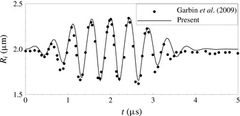
Time evolutions of radius of two bubbles of initial radius
 $2~\unicode[STIX]{x03BC}\text{m}$
and separation distance
 $8~\unicode[STIX]{x03BC}\text{m}$
under ultrasound pulse. The circle symbols are the experimental observation by Garbin et al. (Reference Garbin, Dollet, Overvelde, Cojoc, Di Fabrizio, Van Wijngaarden, Prosperetti, De Jong, Lohse and Versluis2009). The solid line is given in our model.

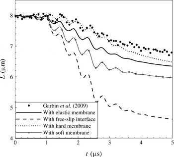
Time evolutions of distance between two bubbles. Circle symbols: experimental results by Garbin et al. (Reference Garbin, Dollet, Overvelde, Cojoc, Di Fabrizio, Van Wijngaarden, Prosperetti, De Jong, Lohse and Versluis2009). Solid line: encapsulated bubbles with normal elastic modulus. Dashed line: gas bubbles with free-slip interfaces. Dotted line: encapsulated bubbles with large elastic modulus. Line with square symbols: encapsulated bubbles with small elastic modulus.

3.1 Membrane effects
To compare with the experimental results by Garbin et al. (Reference Garbin, Dollet, Overvelde, Cojoc, Di Fabrizio, Van Wijngaarden, Prosperetti, De Jong, Lohse and Versluis2009), we consider two bubbles of initial radius
 $2~\unicode[STIX]{x03BC}\text{m}$
and separation distance
 $8~\unicode[STIX]{x03BC}\text{m}$
. An eight-cycle 2.25 MHz ultrasound pulse is applied with an amplitude adjusted to fit the radial variation in the experiment (figure 4). The relative translation is calculated and shows in figure 5 that the two bubbles with the same size move towards each other. Our calculated translations for encapsulated bubbles with elastic membranes (the solid line in figure 5) damp more slowly than those observed in the experiment by Garbin et al. (Reference Garbin, Dollet, Overvelde, Cojoc, Di Fabrizio, Van Wijngaarden, Prosperetti, De Jong, Lohse and Versluis2009). The reason is that the coated bubbles used in Garbin et al. (Reference Garbin, Dollet, Overvelde, Cojoc, Di Fabrizio, Van Wijngaarden, Prosperetti, De Jong, Lohse and Versluis2009) are no-slip at the bubble surface, while our model allows the material points to move along the surface according to a viscoelastic constitutive law. As explained in § 2.6, the drag of an encapsulated bubble with viscoelastic membrane lies between the values of no-slip and free-slip interfaces. If we increase the elastic modulus, the membrane becomes hard and the behaviour of the encapsulated bubble should approach that of a no-slip bubble. As shown by the dotted curve in figure 5, the variation of the distance between the bubbles with large elastic modulus (
 $G_{si}\times 10^{3}$
) approaches that for no-slip bubbles (circle symbols). If we decrease the elastic modulus, the membrane becomes soft and the drag reduces, leading to a larger translational distance, as shown by the line with square symbols in figure 5 for
 $G_{si}\times 10^{-3}$
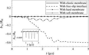
. When we drop the membrane stress and replace it with surface tension, we obtain the result for gas bubbles with a free-slip interface (the dashed line in figure 5), whose damping in translation is much smaller than that of encapsulated bubbles. This confirms that the no-velocity-jump condition for an elastic interface increases the drag significantly. The no-velocity-jump condition induces vorticity generation and thus contributes to the history force in the total drag force. The magnitude of history force depends on the mobility of the material points at the interface, revealed by the tangential displacement
 $b_{ki}$
. Figure 6 shows the time development of
 $b_{1i}$
, denoting the extension or compression along the undeformed interface. The material points on the free-slip interface have a much larger mobility, related to a smaller history force in drag than that of encapsulated bubbles. The comparison among encapsulated bubbles with an elastic membrane (with a normal
 $G_{si}$
), a hard membrane (with
 $G_{si}\times 10^{3}$
) and a soft membrane (with
 $G_{si}\times 10^{-3}$
) reveals that the membrane stress suppresses the mobility of the material points, and this suppression effect is enhanced as the modulus increases. The membrane with a sufficiently large elastic modulus approaches the condition of a no-slip interface. The substantial difference in the tangential movements of material points between encapsulated bubbles and gas bubbles lies in the variation of
 $b_{1i}$
after the ultrasound driving is removed at
 $t=3.56~\unicode[STIX]{x03BC}\text{s}$
. For encapsulated bubbles, the stress in the membrane acts as a restoring force to move the material points back to their equilibrium positions. In these cases,
 $b_{1i}$
returns to zero after
 $t=3.56~\unicode[STIX]{x03BC}\text{s}$
. By comparison, the surface tension in the interface of a gas bubble does not have the restoring effect. Therefore,
 $b_{1i}$
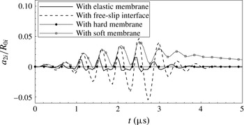
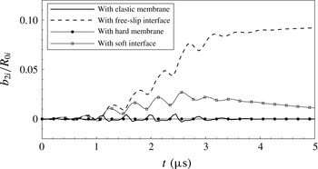
for the gas bubble remains unchanged and will not return to zero after the ultrasound driving stops. For the deformation, we take the shape mode at the lowest order
 $k=2$
as an example and investigate the time developments of
 $a_{2i}$
and
 $b_{2i}$
, as shown in figures 7 and 8, respectively. The amplitudes of
 $a_{2i}$
and
 $b_{2i}$
for the encapsulated bubble with an elastic membrane are smaller than those with free-slip interfaces. The membrane has a stabilizing effect on the interface, making the deformation smaller than the gas bubble. The stabilizing effect becomes more appreciable as the elastic modulus increases. For an extremely large elastic modulus, the model gives a rigid sphere that would not deform. If one sets the membrane parameters to zero and assigns the surface tension, the model is for gas bubbles. By choosing appropriate interface parameters, the model can be used for free-slip, elastic and no-slip interfaces.
Time evolutions of
 $b_{1i}$
for encapsulated bubbles with elastic membranes (solid line), gas bubbles with free-slip interfaces (dashed line), bubbles with hard membranes (line with circle symbols) and bubbles with soft membranes (line with square symbols). Inset: detailed comparison between encapsulated bubbles with elastic and hard membranes.

Time evolutions of
 $a_{2i}$
for encapsulated bubbles with elastic membranes (solid line), gas bubbles with free-slip interfaces (dashed line), bubbles with hard membranes (line with circle symbols) and bubbles with soft membranes (line with square symbols).

Time evolutions of
 $b_{2i}$
for encapsulated bubbles with elastic membranes (solid line), gas bubbles with free-slip interfaces (dashed line), bubbles with hard membranes (line with circle symbols) and bubbles with soft membranes (line with square symbols).

3.2 Validation of the potential part
Under the potential theory, the case of two equal-size bubbles is equivalent to that of a single bubble near a wall which is located at the midpoint between the centres of two bubbles. As a validation of the potential part in our model, we compare our results with the experimental observation by Lauterborn & Bolle (Reference Lauterborn and Bolle1975). The initial radius is
 $R_{01}=R_{02}=2.6\times 10^{-3}~\text{m}$
. The initial distance is
 $3R_{01}$
, equivalent to the distance from the wall being
 $1.5R_{01}$
. This distance is much larger than the boundary layer thickness around the bubble, which is calculated by (2.30) to be
 $\unicode[STIX]{x1D712}/R_{01}<0.1\,\%$
. In addition, the experimental results by Lauterborn & Bolle (Reference Lauterborn and Bolle1975) agree well with the numerical results by Plesset & Chapman (Reference Plesset and Chapman1971), who solved the bubble–wall interaction based on potential flow using the boundary integral method. Plesset & Chapman (Reference Plesset and Chapman1971) assumed that the normal derivative vanishes at the solid wall, implying that their bubble–wall system is equivalent to two equal-size bubbles. The agreement between Lauterborn & Bolle (Reference Lauterborn and Bolle1975) and Plesset & Chapman (Reference Plesset and Chapman1971) indicates the viscous effect is unimportant for the present radius and bubble–wall distance, and it is the added mass inertia and the force due to the pressure obeying the Bernoulli equation that dominate.
The pressure outside the bubbles is set to be
 $p_{\infty }=1\times 10^{5}~\text{Pa}$
, and the pressure inside the bubbles is
 $p_{g01}=p_{g02}=2337~\text{Pa}$
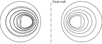
initially. The solid lines in figure 9 show the bubble shapes when
 $\bar{t}=t/[R_{01}(\unicode[STIX]{x1D70C}/\unicode[STIX]{x0394}p)^{1/2}]=0$
, 0.725, 0.825, 0.961, 0.991, 1.016, from larger to smaller shapes. The dotted symbols denote the experimental results at the same times. We can see the results agree well initially. The bubble is elongated in the direction perpendicular to the wall, and moves towards the wall. The results differ slightly at the last two times. Our model is based on a linear approximation for the higher-order shape mode, hence less accurate when the deformation is not small. However, the tendency towards jet formation at the backside of the bubble during collapse is predicted as the third-order shape mode emerges. In general, the agreement with the experimental result is satisfactory.
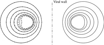
Figure 10 shows the behaviour of two encapsulated bubbles of equal size. We choose the same parameters as those in figure 9, except that the surface tension is neglected and the membrane model is used instead. We calculate the natural frequency of the radial mode using (Liu et al. Reference Liu, Sugiyama, Takagi and Matsumoto2012)
 $$\begin{eqnarray}\unicode[STIX]{x1D714}_{0i}=\sqrt{\frac{3\unicode[STIX]{x1D6E4}p_{\infty }}{\unicode[STIX]{x1D70C}R_{0i}^{2}}+\frac{(6\unicode[STIX]{x1D6E4}-2)\unicode[STIX]{x1D6FE}}{\unicode[STIX]{x1D70C}R_{0i}^{3}}+\frac{12G_{si}}{\unicode[STIX]{x1D70C}R_{0i}^{3}}}.\end{eqnarray}$$
Coincidentally, the natural frequency of this encapsulated bubble is
 $2\unicode[STIX]{x03C0}\times 1258~\text{Hz}$
, close to that of the gas bubble (
 $2\unicode[STIX]{x03C0}\times 1255~\text{Hz}$
). Comparing the shapes at
 $\bar{t}=1.016$
, the deformation of the encapsulated bubble is smaller than that of the gas bubble, implying the interface of the encapsulated bubble is more stable.
Two gas bubbles with equal size.
 $R_{01}=R_{02}=2.6\times 10^{-3}~\text{m}$
. The initial distance between the bubbles is
 $3R_{01}$
;
 $p_{\infty }=1\times 10^{5}~\text{Pa}$
;
 $p_{g01}=p_{g02}=2337~\text{Pa}$
. The solid lines denote the bubble shapes at
 $\bar{t}=0$
, 0.725, 0.825, 0.961, 0.991, 1.016, from larger to smaller shapes. The dotted symbols are the experimental results by Lauterborn & Bolle (Reference Lauterborn and Bolle1975).

Two encapsulated bubbles with equal size.
 $R_{01}=R_{02}=2.6\times 10^{-3}~\text{m}$
. The initial distance between the bubbles is
 $3R_{01}$
;
 $p_{\infty }=1\times 10^{5}~\text{Pa}$
;
 $p_{g01}=p_{g02}=2337~\text{Pa}$
. The solid lines denote the bubble shapes at
 $\bar{t}=0$
, 0.725, 0.825, 0.961, 0.991, 1.016, from larger to smaller shapes. The dotted lines with symbols are the shapes of a gas bubble reproduced from figure 9.

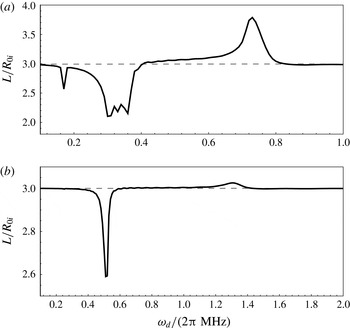
The final distances after 20 driving cycles at different driving frequencies with driving amplitude
 $\unicode[STIX]{x1D700}=0.1$
.
 $R_{01}=10~\unicode[STIX]{x03BC}\text{m}$
,
 $R_{02}=5~\unicode[STIX]{x03BC}\text{m}$
. (a) Gas bubbles, (b) encapsulated bubbles.

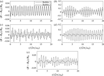
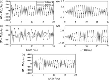
The variations of radius at different driving frequencies for the gas bubbles at
 $\unicode[STIX]{x1D700}=0.1$
.
 $R_{01}=10~\unicode[STIX]{x03BC}\text{m}$
,
 $R_{02}=5~\unicode[STIX]{x03BC}\text{m}$
. (a)
 $\unicode[STIX]{x1D714}_{d}=2\unicode[STIX]{x03C0}\times 0.1~\text{MHz}$
; (b)
 $\unicode[STIX]{x1D714}_{d}=2\unicode[STIX]{x03C0}\times 0.3~\text{MHz}$
; (c)
 $\unicode[STIX]{x1D714}_{d}=2\unicode[STIX]{x03C0}\times 0.5~\text{MHz}$
; (d)
 $\unicode[STIX]{x1D714}_{d}=2\unicode[STIX]{x03C0}\times 0.7~\text{MHz}$
; (e)
 $\unicode[STIX]{x1D714}_{d}=2\unicode[STIX]{x03C0}\times 0.9~\text{MHz}$
.

3.3 Comparison with Bjerknes’ theory
According to Bjerknes’ theory, the two bubbles will move away from each other when the driving frequency is between the two natural frequencies
 $\unicode[STIX]{x1D714}_{01}<\unicode[STIX]{x1D714}_{d}<\unicode[STIX]{x1D714}_{02}$
; and when
 $\unicode[STIX]{x1D714}_{d}<\unicode[STIX]{x1D714}_{01}$
or
 $\unicode[STIX]{x1D714}_{d}>\unicode[STIX]{x1D714}_{02}$
, the two bubbles will move towards each other. We choose two bubbles with
 $R_{01}=10~\unicode[STIX]{x03BC}\text{m}$
and
 $R_{02}=5~\unicode[STIX]{x03BC}\text{m}$
and set their initial distance as
 $3R_{01}$
. A driving pressure characterized by a dimensionless amplitude
 $\unicode[STIX]{x1D700}$
and a driving frequency
 $\unicode[STIX]{x1D714}_{d}$
is applied:
 $$\begin{eqnarray}p_{\infty }=p_{0}(1+\unicode[STIX]{x1D700}\sin \unicode[STIX]{x1D714}_{d}t),\end{eqnarray}$$
where the ambient pressure
 $p_{0}$
is set as
 $1\times 10^{5}~\text{Pa}$
. We plot the final distances between the two bubbles after 20 driving cycles by sweeping the driving frequency in figure 11. Here the driving amplitude is
 $\unicode[STIX]{x1D700}=0.1$
. Figure 11(a) is the result for gas bubbles, and figure 11(b) for encapsulated bubbles. It is noted that the zeroth-order natural frequencies of the gas bubbles are
 $\unicode[STIX]{x1D714}_{01}=2\unicode[STIX]{x03C0}\times 0.34~\text{MHz}$
and
 $\unicode[STIX]{x1D714}_{02}=2\unicode[STIX]{x03C0}\times 0.72~\text{MHz}$
, respectively. From figure 11(a), we can see the two bubbles are attracted to each other when the driving frequency is less than both natural frequencies. When the driving frequency approaches the smaller natural frequency, i.e.
 $\unicode[STIX]{x1D714}_{d}=\unicode[STIX]{x1D714}_{01}$
, the distance reaches a minimum. After this minimum, the relative translational motion becomes repulsive. As the driving frequency increases to the vicinity of the larger natural frequency, i.e.
 $\unicode[STIX]{x1D714}_{d}=\unicode[STIX]{x1D714}_{02}$
, the two bubbles repel each other to the maximal distance. After this maximum, the bubbles return to being attractive. This picture agrees well with Bjerknes’ theory. Figure 11(a) shows that the resonance in radial oscillation leads to an extreme translation. At the same time, the resonance at subharmonics causes a secondary extreme translation. In figure 11(a), there is a local minimum near
 $2\unicode[STIX]{x03C0}\times 0.17~\text{MHz}$
, which is half of the zeroth-order natural frequency
 $\unicode[STIX]{x1D714}_{01}$
. Half of another natural frequency (
 $\unicode[STIX]{x1D714}_{02}$
) is
 $2\unicode[STIX]{x03C0}\times 0.36~\text{MHz}$
, close to
 $\unicode[STIX]{x1D714}_{01}=2\unicode[STIX]{x03C0}\times 0.34~\text{MHz}$
, which explains why the minimum near
 $2\unicode[STIX]{x03C0}\times 0.34~\text{MHz}$
has a broad spread to around
 $2\unicode[STIX]{x03C0}\times 0.36~\text{MHz}$
.
Figure 11(b) shows the results for encapsulated bubbles. Under the same driving amplitude, the translational distances of encapsulated bubbles are much smaller than those of gas bubbles. Our calculated zeroth-order natural frequencies of the two encapsulated bubbles are
 $\unicode[STIX]{x1D714}_{01}=2\unicode[STIX]{x03C0}\times 0.51~\text{MHz}$
and
 $\unicode[STIX]{x1D714}_{02}=2\unicode[STIX]{x03C0}\times 1.28~\text{MHz}$
, respectively. The minimal distance occurs near
 $\unicode[STIX]{x1D714}_{01}=2\unicode[STIX]{x03C0}\times 0.51~\text{MHz}$
and the maximum occurs near
 $\unicode[STIX]{x1D714}_{02}=2\unicode[STIX]{x03C0}\times 1.28~\text{MHz}$
. The behaviour in translation follows the prediction by the Bjerknes theory. Different from the gas bubble case, no local minimum appears near subharmonic resonance for encapsulated bubbles, which is attributed to the damping effects due to the encapsulating membrane, making the behaviour of encapsulated bubbles more stable.
Bjerknes’ theory also states that the bubbles move towards each other when oscillating in phase (
 $\unicode[STIX]{x0394}\unicode[STIX]{x1D719}<\unicode[STIX]{x03C0}/2$
or
 $\unicode[STIX]{x0394}\unicode[STIX]{x1D719}>3\unicode[STIX]{x03C0}/2$
); otherwise, they repel each other when oscillating out of phase (
 $\unicode[STIX]{x03C0}/2<\unicode[STIX]{x0394}\unicode[STIX]{x1D719}<3\unicode[STIX]{x03C0}/2$
), where
 $\unicode[STIX]{x0394}\unicode[STIX]{x1D719}$
is the difference in phase angle. To examine the effects of the phase difference, we choose a set of driving frequencies: smaller than
 $\unicode[STIX]{x1D714}_{01}$
, near
 $\unicode[STIX]{x1D714}_{01}$
, between
 $\unicode[STIX]{x1D714}_{01}$
and
 $\unicode[STIX]{x1D714}_{02}$
, near
 $\unicode[STIX]{x1D714}_{02}$
, and larger than
 $\unicode[STIX]{x1D714}_{02}$
, that is,
 $\unicode[STIX]{x1D714}_{d}/2\unicode[STIX]{x03C0}=0.1$
, 0.3, 0.5, 0.7, 0.9 MHz for gas bubbles and
 $\unicode[STIX]{x1D714}_{d}/2\unicode[STIX]{x03C0}=0.3$
, 0.5, 0.8, 1.3, 1.5 MHz for encapsulated bubbles. The time evolutions of radius are plotted in figures 12 and 13, respectively. We can see the in-phase oscillations in figures 12(a), 12(b), 13(a) and 13(b), corresponding to the attractive motion we have observed in figure 11. For the driving frequencies greater than both natural frequencies,
 $\unicode[STIX]{x1D714}_{d}/2\unicode[STIX]{x03C0}=0.9~\text{MHz}$
for gas bubbles and
 $\unicode[STIX]{x1D714}_{d}/2\unicode[STIX]{x03C0}=1.5~\text{MHz}$
for encapsulated bubbles, the bubbles exhibit slight translation even when the two bubbles oscillate out of phase. This is perhaps due to the fact that the bubbles do not have enough time to move from their initial positions and keep a stable separation under such high driving frequencies, relating to ‘bubble grape’, which is supposed to form at high frequency (Harkin et al.
Reference Harkin, Kaper and Nadim2001). For other cases (figures 12
c, 12
d, 13
c and 13
d), the two bubbles oscillate out of phase and consequently move away from each other. These results show that the phase difference comes from the nonlinear oscillation subjected to different driving frequencies, which are responsible for the attraction or repulsion of the two bubbles.
The variations of radius at different driving frequencies for the encapsulated bubbles at
 $\unicode[STIX]{x1D700}=0.1$
.
 $R_{01}=10~\unicode[STIX]{x03BC}\text{m}$
,
 $R_{02}=5~\unicode[STIX]{x03BC}\text{m}$
. (a)
 $\unicode[STIX]{x1D714}_{d}=2\unicode[STIX]{x03C0}\times 0.3~\text{MHz}$
; (b)
 $\unicode[STIX]{x1D714}_{d}=2\unicode[STIX]{x03C0}\times 0.5~\text{MHz}$
; (c)
 $\unicode[STIX]{x1D714}_{d}=2\unicode[STIX]{x03C0}\times 0.8~\text{MHz}$
; (d)
 $\unicode[STIX]{x1D714}_{d}=2\unicode[STIX]{x03C0}\times 1.3~\text{MHz}$
; (e)
 $\unicode[STIX]{x1D714}_{d}=2\unicode[STIX]{x03C0}\times 1.5~\text{MHz}$
.

3.4 Contributions of different forces
In this section, we investigate the roles of the different forces in (2.49)–(2.54). We choose the driving frequency
 $\unicode[STIX]{x1D714}_{d}=2\unicode[STIX]{x03C0}\times 0.3~\text{MHz}$
for gas bubbles and
 $\unicode[STIX]{x1D714}_{d}=2\unicode[STIX]{x03C0}\times 0.5~\text{MHz}$
for encapsulated bubbles. Under these driving frequencies, the larger bubble experiences radial resonance and the two bubbles exhibit maximal attractive motion. The forces are averaged over a driving cycle:
 $$\begin{eqnarray}\langle F.\rangle =\frac{\unicode[STIX]{x1D714}_{d}}{2\unicode[STIX]{x03C0}}\int _{0}^{2\unicode[STIX]{x03C0}/\unicode[STIX]{x1D714}_{d}}F.\,\text{d}t,\end{eqnarray}$$
so are the distances and the velocities. Figures 14(a) and 14(b) show the time evolutions of the averaged forces exerting on bubble 1 (the larger bubble) for gas bubbles and encapsulated bubbles, respectively; figures 14(c) and 14(d) are for bubble 2 (the smaller bubble). Figures 14(e) and 14(f) show the respective variations of distances for gas and encapsulated bubbles, and figures 14(g) and 14(h) show the variations of velocities.
The time evolutions of forces acting on the bubbles, the distance between the two bubbles and the velocity of each bubble. (a,c,e,g) Gas bubbles at
 $\unicode[STIX]{x1D714}_{d}=2\unicode[STIX]{x03C0}\times 0.3~\text{MHz}$
. (b,d,f,h) Encapsulated bubbles at
 $\unicode[STIX]{x1D714}_{d}=2\unicode[STIX]{x03C0}\times 0.5~\text{MHz}$
. (a,b) Forces on the larger bubbles (bubble 1). (c,d) Forces on the smaller bubbles (bubble 2). (e,f) Distance variations. (g,h) Variation of velocity of each bubble.

As shown in figures 14(a) and 14(c), and figures 14(b) and 14(d), the time-averaged Bjerknes forces follow the envelopes of radial variation in figures 12(b) and 13(b), respectively. This is natural since the Bjerknes force is due to the radial oscillation of the nearby bubble. In general,
 $F_{B1}$
is positive, and
 $F_{B2}$
is negative. Referred to the coordinates we established in figure 1, the two bubbles move towards each other and lead to a decreasing distance (figures 14
e and 14
f). The forces with opposite sign of the Bjerknes force behave as a drag. For gas bubbles, the drag mainly comes from the viscous forces
 $F_{\unicode[STIX]{x1D707}i}$
, in which the quasisteady drag force
 $12\unicode[STIX]{x03C0}\unicode[STIX]{x1D707}_{l}R_{i}v_{ri}$
dominates. For encapsulated bubbles, on the other hand, the drag is mainly from the membrane forces
 $F_{mi}$
, contributing to the history force through the tangential dynamic boundary condition (2.46).
 $F_{h1i}$
for bubble 1 is a drag, since its sign is opposite to the Bjerknes force, resulting from the translation of bubble 2 (the smaller bubble), which has a larger (absolute) velocity than the larger bubble (bubble 1) (figures 14
g and 14
h). It is understandable, since the magnitudes of forces of the two bubbles are comparable (figures 14
a and 14
c, figures 14
b and 14
d), so that the smaller bubble experiences a larger acceleration and velocity. This larger velocity of bubble 2 contributes to the force
 $F_{h1i}$
on bubble 1, which is related to the Bjerknes-like force due to the translation of the nearby bubble. The other higher-order forces
 $F_{h2i}$
and
 $F_{h3i}$
are small, suggesting that the coupling effect of the translation and the radial oscillation of the nearby bubble is not important, and the bubbles do not exhibit appreciable deformation in the present cases.
The presence of the membrane does not necessarily damp radial oscillations. The amplitude of radial oscillation depends on its frequency. At resonance, the oscillatory amplitude of the encapsulated bubble is comparable to that of the gas bubble, as shown in figures 12(b) and 13(b). Determined by the radial oscillation of the nearby bubble, the magnitudes of the Bjerknes forces of encapsulated bubbles are thereby of the same order as those of gas bubbles, as revealed by comparing figures 14(a,c) and figures 14(b,d). However, the no-velocity-jump condition on membranes contributes significantly to the viscous drag, which has been explained in § 2.6, as it increases the viscous dissipation. The expression for the viscous drag (2.57) includes the history force, which was shown to be important for encapsulated bubbles in the previous sections and by Garbin et al. (Reference Garbin, Dollet, Overvelde, Cojoc, Di Fabrizio, Van Wijngaarden, Prosperetti, De Jong, Lohse and Versluis2009). Therefore, the translational distances of encapsulated bubbles are smaller than those of gas bubbles even when they experience comparative radial oscillations. In addition, due to the smaller translations of encapsulated bubbles compared with gas bubbles, the boundary layers, which are more important for encapsulated bubbles with no-velocity-jump condition than for gas bubbles with free-slip condition, do not overlap. This ensures that our model of assumption of potential flow with viscous correction remains valid.
4 Conclusion
In this paper, we have established a theoretical model for the interaction of two encapsulated bubbles that considers their deformations. The in-plane stress and bending moments of an viscoelastic membrane are balanced by the hydrodynamic traction across the bubble interface, giving dynamic equations for the radial pulsation, translation and shape oscillation. Due to the no-velocity-jump condition on the membrane, the viscous dissipation is included through a vorticity equation in the toroidal direction. The derived viscous drag includes the quasisteady drag force and the history force, which is validated by the solution of the unsteady Stokes equation.
Our model is suitable for bubbles with free-slip, viscoelastic or no-slip interfaces. By setting the membrane parameters to zero and replacing it with the surface tension, our model can be used for gas bubbles with a free-slip surface. Choosing a large membrane elasticity modulus generates a solution to rigid bubbles with a no-slip interface. Choosing appropriate membrane parameters, we obtain the solution for encapsulated bubbles with a viscoelastic membrane.
The membrane effects of two encapsulated bubbles of the same size under ultrasound pulse are investigated. Their translational distances lie between the range of two free-slip gas bubbles and two no-slip bubbles studied in the experiment by Garbin et al. (Reference Garbin, Dollet, Overvelde, Cojoc, Di Fabrizio, Van Wijngaarden, Prosperetti, De Jong, Lohse and Versluis2009). This is due to the fact that the encapsulated bubbles with elastic membranes allow the material points to move along the interface according to a viscoelastic law.
The potential part in the present model is validated by comparing our results with the experimental results of Lauterborn & Bolle (Reference Lauterborn and Bolle1975) and numerical results of Plesset & Chapman (Reference Plesset and Chapman1971). The encapsulated bubble is more stable in resisting shape oscillations.
Consistent with Bjerknes’ theory, two bubbles move against or away from each other when the driving frequency is beyond or between their natural frequencies. Nonlinearity in radial oscillation causes a phase difference, which leads to attraction when in phase and repulsion when out of phase, also consistent with the predictions of Bjerknes’ theory. By comparison, encapsulated bubbles exhibit more damping in their translational motion than gas bubbles. For gas bubbles, the drag comes mainly from the quasisteady viscous force. For encapsulated bubbles, the history force, which results from the vorticity diffusion induced by the no-velocity-jump interface, contributes significantly to the drag, generating additional damping in the translation.
Acknowledgements
The authors are grateful to Professors H. Takahira and H. Huang for fruitful discussions. The authors are also grateful to the reviewers for their useful comments and suggestions. This work was supported by the National Natural Science Foundation of China (11302128).
Appendix A. Orthogonal relations of the Legendre polynomials
The orthogonal relations of the Legendre polynomials are used throughout this paper. The Legendre polynomials
 $P_{k}(\cos \unicode[STIX]{x1D703}_{i})$
and
 $P_{k}^{1}(\cos \unicode[STIX]{x1D703}_{i})$
are simply written as
 $P_{k}$
and
 $P_{k}^{1}$
in this appendix. We have
 $$\begin{eqnarray}\displaystyle & \displaystyle \int _{-1}^{1}P_{k}P_{l}\,\text{d}(\cos \unicode[STIX]{x1D703}_{i})=0,\quad \text{when}~k\not =l, & \displaystyle\end{eqnarray}$$
 $$\begin{eqnarray}\displaystyle & \displaystyle (P_{1})^{2}={\textstyle \frac{1}{3}}(P_{0}+2P_{2}), & \displaystyle\end{eqnarray}$$
 $$\begin{eqnarray}\displaystyle & \displaystyle (P_{1}^{1})^{2}={\textstyle \frac{2}{3}}(P_{0}-P_{2}), & \displaystyle\end{eqnarray}$$
 $$\begin{eqnarray}\displaystyle & \displaystyle \mathop{\sum }_{k=2}^{\infty }a_{k}P_{1}P_{k}=\mathop{\sum }_{k=1}^{\infty }\frac{k+1}{2k+3}a_{k+1}P_{k}+\mathop{\sum }_{k=3}^{\infty }\frac{k}{2k-1}a_{k-1}P_{k}, & \displaystyle\end{eqnarray}$$
 $$\begin{eqnarray}\displaystyle & \displaystyle \mathop{\sum }_{k=2}^{\infty }a_{k}P_{1}^{1}P_{k}^{1}=\mathop{\sum }_{k=1}^{\infty }\frac{(k+1)(k+2)}{2k+3}a_{k+1}P_{k}-\mathop{\sum }_{k=3}^{\infty }\frac{k(k-1)}{2k-1}a_{k-1}P_{k}. & \displaystyle\end{eqnarray}$$
Appendix B. Mechanics of the membrane
The hydrodynamic traction across a bubble interface is balanced by the stress exerted on the membrane. The membrane stress is given by the surface divergence of the elastic tension tensor. The tension of the encapsulating membrane includes the in-plane tension and bending moment. We can write the membrane stress
 $\boldsymbol{F}_{i}$
as (Green & Adkins Reference Green and Adkins1960):
 $$\begin{eqnarray}\boldsymbol{F}_{i}=-(\unicode[STIX]{x1D64B}_{i}\boldsymbol{\cdot }\unicode[STIX]{x1D735}_{i})\boldsymbol{\cdot }(\unicode[STIX]{x1D749}_{i}+\boldsymbol{q}_{i}\boldsymbol{n}_{i}),\end{eqnarray}$$
where
 $\unicode[STIX]{x1D749}_{i}$
is the in-plane stress and we express it in the form of principal components in spherical coordinates:
 $$\begin{eqnarray}\unicode[STIX]{x1D749}_{i}=\unicode[STIX]{x1D70F}_{\unicode[STIX]{x1D703}i}\boldsymbol{e}_{\unicode[STIX]{x1D703}i}\boldsymbol{e}_{\unicode[STIX]{x1D703}i}+\unicode[STIX]{x1D70F}_{\unicode[STIX]{x1D719}i}\boldsymbol{e}_{\unicode[STIX]{x1D719}i}\boldsymbol{e}_{\unicode[STIX]{x1D719}i}.\end{eqnarray}$$
The torque balance with respect to an arbitrary point provides the relationship between the transverse shear tension
 $\boldsymbol{q}_{i}$
and the bending moment
 $\boldsymbol{m}_{i}$
:
 $$\begin{eqnarray}\boldsymbol{q}_{i}=[(\unicode[STIX]{x1D64B}_{i}\boldsymbol{\cdot }\unicode[STIX]{x1D735}_{i})\boldsymbol{\cdot }\boldsymbol{m}_{i}]\boldsymbol{\cdot }\unicode[STIX]{x1D64B}_{i}.\end{eqnarray}$$
Similarly, we express
 $\boldsymbol{m}_{i}$
in the form of principal components:
 $$\begin{eqnarray}\boldsymbol{m}_{i}=m_{\unicode[STIX]{x1D703}i}\boldsymbol{e}_{\unicode[STIX]{x1D703}i}\boldsymbol{e}_{\unicode[STIX]{x1D703}i}+m_{\unicode[STIX]{x1D719}i}\boldsymbol{e}_{\unicode[STIX]{x1D719}i}\boldsymbol{e}_{\unicode[STIX]{x1D719}i}.\end{eqnarray}$$
Substituting (B 2) and (B 4) into (B 1), along with the expression of surface projection operator
 $\unicode[STIX]{x1D64B}_{i}=\unicode[STIX]{x1D644}_{i}-\boldsymbol{n}_{i}\boldsymbol{n}_{i}$
and the unit normal vector
 $\boldsymbol{n}_{i}$
(2.17) we have derived in § 2.2, the membrane stress
 $\boldsymbol{F}_{i}$
becomes:
 $$\begin{eqnarray}\displaystyle \boldsymbol{F}_{i}=F_{ni}\boldsymbol{e}_{ri}+F_{ti}\boldsymbol{e}_{\unicode[STIX]{x1D703}i}, & & \displaystyle\end{eqnarray}$$
where the membrane stress in the normal direction is
 $$\begin{eqnarray}\displaystyle F_{ni}=\frac{1}{r_{i}}(\unicode[STIX]{x1D70F}_{\unicode[STIX]{x1D703}i}+\unicode[STIX]{x1D70F}_{\unicode[STIX]{x1D719}i})-\frac{q_{i}\cos \unicode[STIX]{x1D703}_{i}}{r_{i}\sin \unicode[STIX]{x1D703}_{i}}-\frac{1}{r_{i}}\frac{\unicode[STIX]{x2202}q_{i}}{\unicode[STIX]{x2202}\unicode[STIX]{x1D703}i}, & & \displaystyle\end{eqnarray}$$
and that in tangential direction is
 $$\begin{eqnarray}\displaystyle F_{ti}=\frac{\cos \unicode[STIX]{x1D703}_{i}}{r\sin \unicode[STIX]{x1D703}_{i}}(\unicode[STIX]{x1D70F}_{\unicode[STIX]{x1D719}i}-\unicode[STIX]{x1D70F}_{\unicode[STIX]{x1D703}i})-\frac{q_{i}}{r_{i}}-\frac{1}{r_{i}}\frac{\unicode[STIX]{x2202}\unicode[STIX]{x1D70F}_{\unicode[STIX]{x1D703}i}}{\unicode[STIX]{x2202}\unicode[STIX]{x1D703}i}+\frac{\unicode[STIX]{x1D70F}_{\unicode[STIX]{x1D703}i}}{r_{i}^{2}}\mathop{\sum }_{k=2}^{\infty }a_{ki}P_{k}^{1}(\cos \unicode[STIX]{x1D703}_{i}), & & \displaystyle\end{eqnarray}$$
where
 $$\begin{eqnarray}\displaystyle q_{i}=\frac{1}{r_{i}}\frac{\unicode[STIX]{x2202}m_{\unicode[STIX]{x1D703}i}}{\unicode[STIX]{x2202}\unicode[STIX]{x1D703}_{i}}+\frac{\cos \unicode[STIX]{x1D703}_{i}}{r_{i}\sin \unicode[STIX]{x1D703}_{i}}(m_{\unicode[STIX]{x1D703}i}-m_{\unicode[STIX]{x1D719}i}). & & \displaystyle\end{eqnarray}$$
We employ a constitutive law of a viscoelastic membrane to connect the stress and the strain of the membrane. For the elastic part, we adopt the neo-Hookean law (Mooney Reference Mooney1940) as an example. It is described by a Helmholtz strain energy function
 $W_{si}$
, which is defined by the two principal strains
 $\unicode[STIX]{x1D706}_{\unicode[STIX]{x1D703}i}$
and
 $\unicode[STIX]{x1D706}_{\unicode[STIX]{x1D719}i}$
and the surface modulus of elasticity
 $G_{si}$
, i.e.
 $$\begin{eqnarray}W_{si}=\frac{G_{si}}{2}\left(\unicode[STIX]{x1D706}_{\unicode[STIX]{x1D703}i}^{2}+\unicode[STIX]{x1D706}_{\unicode[STIX]{x1D719}i}^{2}+\frac{1}{\unicode[STIX]{x1D706}_{\unicode[STIX]{x1D703}i}^{2}\unicode[STIX]{x1D706}_{\unicode[STIX]{x1D719}i}^{2}}-3\right).\end{eqnarray}$$
We regard the viscous part as a linear resistance to the strain rate, characterized by the viscous coefficient of the membrane
 $\unicode[STIX]{x1D707}_{si}$
. Combined with the elastic and viscous parts, the in-plane stresses are written as
 $$\begin{eqnarray}\unicode[STIX]{x1D70F}_{\unicode[STIX]{x1D703}i}=\frac{1}{\unicode[STIX]{x1D706}_{\unicode[STIX]{x1D719}i}}\frac{\unicode[STIX]{x2202}W_{si}}{\unicode[STIX]{x2202}\unicode[STIX]{x1D706}_{\unicode[STIX]{x1D703}i}}+2\unicode[STIX]{x1D707}_{si}\frac{1}{\unicode[STIX]{x1D706}_{\unicode[STIX]{x1D703}i}}\frac{\unicode[STIX]{x2202}\unicode[STIX]{x1D706}_{\unicode[STIX]{x1D703}i}}{\unicode[STIX]{x2202}t},\end{eqnarray}$$
and
 $$\begin{eqnarray}\unicode[STIX]{x1D70F}_{\unicode[STIX]{x1D719}i}=\frac{1}{\unicode[STIX]{x1D706}_{\unicode[STIX]{x1D703}i}}\frac{\unicode[STIX]{x2202}W_{si}}{\unicode[STIX]{x2202}\unicode[STIX]{x1D706}_{\unicode[STIX]{x1D719}i}}+2\unicode[STIX]{x1D707}_{si}\frac{1}{\unicode[STIX]{x1D706}_{\unicode[STIX]{x1D719}i}}\frac{\unicode[STIX]{x2202}\unicode[STIX]{x1D706}_{\unicode[STIX]{x1D719}i}}{\unicode[STIX]{x2202}t}.\end{eqnarray}$$
The bending moment is determined by the two principal curvatures of the surface. Similarly, it is described by a bending strain energy function
 $W_{bi}$
. Here we adopt Love’s law (Love Reference Love1888):
 $$\begin{eqnarray}W_{bi}=\frac{G_{bi}}{2}(K_{\unicode[STIX]{x1D703}i}^{2}+2\unicode[STIX]{x1D710}K_{\unicode[STIX]{x1D703}i}K_{\unicode[STIX]{x1D719}i}+K_{\unicode[STIX]{x1D719}i}^{2}),\end{eqnarray}$$
where
 $G_{bi}$
denotes the bending modulus and
 $\unicode[STIX]{x1D710}$
the Poisson ratio.
 $K_{\unicode[STIX]{x1D703}i}$
and
 $K_{\unicode[STIX]{x1D719}i}$
are bending strains defined under the assumption of small deformation:
 $$\begin{eqnarray}K_{\unicode[STIX]{x1D703}i}=\unicode[STIX]{x1D706}_{\unicode[STIX]{x1D703}i}\unicode[STIX]{x1D705}_{\unicode[STIX]{x1D703}}-\frac{1}{R_{0i}},\quad K_{\unicode[STIX]{x1D719}i}=\unicode[STIX]{x1D706}_{\unicode[STIX]{x1D719}i}\unicode[STIX]{x1D705}_{\unicode[STIX]{x1D719}i}-\frac{1}{R_{0i}}.\end{eqnarray}$$
Then the bending moments are obtained as
 $$\begin{eqnarray}m_{\unicode[STIX]{x1D703}i}=\frac{1}{\unicode[STIX]{x1D706}_{\unicode[STIX]{x1D719}i}}\frac{\unicode[STIX]{x2202}W_{bi}}{\unicode[STIX]{x2202}K_{\unicode[STIX]{x1D703}i}},\end{eqnarray}$$
and
 $$\begin{eqnarray}m_{\unicode[STIX]{x1D719}i}=\frac{1}{\unicode[STIX]{x1D706}_{\unicode[STIX]{x1D703}i}}\frac{\unicode[STIX]{x2202}W_{bi}}{\unicode[STIX]{x2202}K_{\unicode[STIX]{x1D719}i}}.\end{eqnarray}$$
Substituting the strain energy function (B 9) into (B 10) and (B 11), and the bending energy function (B 12) into (B 14) and (B 15), we obtain the constitutive equations of in-plane stresses and bending moments. Combined with the expressions for the strains and curvatures we derived in § 2.2, we obtain the membrane stresses in the tangential and normal directions in terms of the surface positions (2.38) and (2.39).
Appendix C. Drag force of a spherical encapsulated bubble in an oscillatory motion in Stokes flow
We investigate a spherical encapsulated bubble translating in an oscillatory pattern under Stokes flow to cross-check the viscous drag that has been derived in the translation equation (2.48). The derivation is based on Landau & Lifshitz (Reference Landau and Lifshitz1987) and includes the encapsulating membrane as an extension. Hereafter we remove the subscripts
 $i$
and
 $j$
for brevity and neglect the variation of the bubble radius
 $R$
for simplicity. The translational velocity of the bubble centroid is
 $\boldsymbol{v}=v\boldsymbol{e}_{z}$
. The velocity and pressure induced by the oscillatory motion are decomposed into a potential part (with subscript
 $p$
) and a viscous correction (with subscript
 $v$
), written as
 $$\begin{eqnarray}\displaystyle \boldsymbol{u}=(\boldsymbol{u}_{p}+\boldsymbol{u}_{v})\text{e}^{\text{i}\unicode[STIX]{x1D714}t},\quad p=(p_{p}+p_{v})\text{e}^{\text{i}\unicode[STIX]{x1D714}t}, & & \displaystyle\end{eqnarray}$$
which satisfy the unsteady Stokes equation:
 $$\begin{eqnarray}\unicode[STIX]{x1D70C}\frac{\unicode[STIX]{x2202}\boldsymbol{u}}{\unicode[STIX]{x2202}t}=-\unicode[STIX]{x1D735}p+\unicode[STIX]{x1D707}\unicode[STIX]{x1D6FB}^{2}\boldsymbol{u}.\end{eqnarray}$$
The potential part satisfies the unsteady Stokes equation with the viscous term zero, from which we obtain
 $$\begin{eqnarray}\displaystyle & \displaystyle \boldsymbol{u}_{p}=\frac{R^{3}v}{r^{3}}\cos \unicode[STIX]{x1D703}\boldsymbol{e}_{r}+\frac{R^{3}v}{2r^{3}}\sin \unicode[STIX]{x1D703}\boldsymbol{e}_{\unicode[STIX]{x1D703}}, & \displaystyle\end{eqnarray}$$
 $$\begin{eqnarray}\displaystyle & \displaystyle p_{p}=\frac{\text{i}\unicode[STIX]{x1D714}\unicode[STIX]{x1D70C}R^{3}v}{2r^{2}}\cos \unicode[STIX]{x1D703}. & \displaystyle\end{eqnarray}$$
For the viscous correction part, we introduce the Stokes stream function
 $\unicode[STIX]{x1D713}=\hat{\unicode[STIX]{x1D713}}\sin ^{2}\unicode[STIX]{x1D703}$
. The solution to the Stokes equation with the kinematic condition (
 $u_{vr}=0$
at
 $r=R$
) and the regularity at infinity is
 $$\begin{eqnarray}\hat{\unicode[STIX]{x1D713}}=-\frac{C\unicode[STIX]{x1D701}(\unicode[STIX]{x1D701}R+1)\text{e}^{-\unicode[STIX]{x1D701}R}}{r}+\frac{C\unicode[STIX]{x1D701}(\unicode[STIX]{x1D701}r+1)\text{e}^{-\unicode[STIX]{x1D701}r}}{r},\end{eqnarray}$$
where
 $\unicode[STIX]{x1D701}=\sqrt{\text{i }\unicode[STIX]{x1D714}\unicode[STIX]{x1D70C}/\unicode[STIX]{x1D707}}$
, relating to the Womersley number. Here we consider the case with high Womersley number, which has been justified in § 2.6. The velocity and pressure of viscous corrections are obtained therefrom:
 $$\begin{eqnarray}\displaystyle \boldsymbol{u}_{v} & = & \displaystyle \frac{2\hat{\unicode[STIX]{x1D713}}}{r^{2}}\cos \unicode[STIX]{x1D703}\boldsymbol{e}_{r}-\frac{1}{r}\frac{\text{d}\hat{\unicode[STIX]{x1D713}}}{\text{d}r}\sin \unicode[STIX]{x1D703}\boldsymbol{e}_{\unicode[STIX]{x1D703}},\end{eqnarray}$$
 $$\begin{eqnarray}\displaystyle p_{v} & = & \displaystyle -\frac{C\unicode[STIX]{x1D707}_{l}\unicode[STIX]{x1D701}^{3}(\unicode[STIX]{x1D701}R+1)\text{e}^{-\unicode[STIX]{x1D701}R}}{r^{2}}\cos \unicode[STIX]{x1D703}.\end{eqnarray}$$
Next we calculate the force acting on the bubble by integrating the stress around the surface and obtain
 $$\begin{eqnarray}\displaystyle F=-F_{a}-F_{D}, & & \displaystyle\end{eqnarray}$$
where
 $F_{a}$
is the added mass inertia:
 $$\begin{eqnarray}F_{a}=\text{i}\unicode[STIX]{x1D714}\frac{2\unicode[STIX]{x03C0}\unicode[STIX]{x1D70C}R^{3}v}{3},\end{eqnarray}$$
and
 $F_{D}$
is the drag force:
 $$\begin{eqnarray}F_{D}=-4\unicode[STIX]{x03C0}C\unicode[STIX]{x1D707}_{l}\unicode[STIX]{x1D701}^{3}(\unicode[STIX]{x1D701}R+1)\text{e}^{-\unicode[STIX]{x1D701}R}.\end{eqnarray}$$
The tangential dynamic boundary condition at the bubble interface (2.35) is written as
 $$\begin{eqnarray}3\unicode[STIX]{x1D707}_{l}\frac{v}{R}+C\unicode[STIX]{x1D707}_{l}\text{e}^{-\unicode[STIX]{x1D701}R}\frac{\unicode[STIX]{x1D701}^{3}}{R^{2}}(3+R\unicode[STIX]{x1D701})=(6G_{s}+2\unicode[STIX]{x1D707}_{s}\text{i}\unicode[STIX]{x1D714})\frac{\hat{b}}{R^{2}},\end{eqnarray}$$
where the right-hand side is the tangential membrane stress at the mode of
 $P_{1}^{1}(\cos \unicode[STIX]{x1D703})$
(ref. (2.38)). Here we neglect the bending moment for simplicity and define
 $b_{1}\triangleq \hat{b}\text{e}^{\text{i}\unicode[STIX]{x1D714}t}$
.
The continuity of tangential velocity at the bubble interface implies
 $$\begin{eqnarray}\frac{v}{2}+\frac{C\unicode[STIX]{x1D701}^{3}\text{e}^{-\unicode[STIX]{x1D701}R}}{R}=-v-\text{i}\unicode[STIX]{x1D714}\hat{b}.\end{eqnarray}$$
Eliminating
 $\hat{b}$
in (C 11) and (C 12), we obtain:
 $$\begin{eqnarray}C=-\frac{3\text{e}^{\unicode[STIX]{x1D701}R}Rv(\unicode[STIX]{x1D6F6}+2R)}{2\unicode[STIX]{x1D701}^{3}(\unicode[STIX]{x1D6F6}+\unicode[STIX]{x1D701}R^{2}+3R)},\end{eqnarray}$$
where
 $$\begin{eqnarray}\unicode[STIX]{x1D6F6}=\frac{6G_{s}+2\unicode[STIX]{x1D707}_{s}\text{i}\unicode[STIX]{x1D714}}{\text{i}\unicode[STIX]{x1D714}\unicode[STIX]{x1D707}_{l}}.\end{eqnarray}$$
Substituting (C 13) into (C 10), we obtain the drag force for an encapsulated bubble. If
 $G_{s}$
and
 $\unicode[STIX]{x1D707}_{s}$
approach infinity, the bubble is equivalent to a rigid sphere, for which we denote
 $C$
as
 $C_{r}$
, and (C 13) becomes
 $$\begin{eqnarray}C_{r}=-\frac{3Rv\text{e}^{\unicode[STIX]{x1D701}R}}{2\unicode[STIX]{x1D701}^{3}}.\end{eqnarray}$$
If
 $G_{s}=\unicode[STIX]{x1D707}_{s}=0$
, the bubble is a gas bubble with the shear stress at the interface zero, for which
 $C$
(denoted as
 $C_{g}$
) reduces to
 $$\begin{eqnarray}C_{g}=-\frac{3Rv\text{e}^{\unicode[STIX]{x1D701}R}}{\unicode[STIX]{x1D701}^{3}(\unicode[STIX]{x1D701}R+3)}.\end{eqnarray}$$
Substituting
 $C$
with (C 15) for a rigid sphere, or with (C 16) for a gas bubble, we obtain the drag force at high Womersley number (i.e.
 $|\unicode[STIX]{x1D701}|\gg 1$
):
 $$\begin{eqnarray}\displaystyle & \displaystyle \text{for a rigid sphere},\quad F_{D}\sim 6\unicode[STIX]{x03C0}\unicode[STIX]{x1D707}vR^{2}\unicode[STIX]{x1D701}+6\unicode[STIX]{x03C0}\unicode[STIX]{x1D707}Rv; & \displaystyle\end{eqnarray}$$
 $$\begin{eqnarray}\displaystyle & \displaystyle \text{for a shear-free bubble},\quad F_{D}\sim 12\unicode[STIX]{x03C0}\unicode[STIX]{x1D707}Rv+O(\unicode[STIX]{x1D701}^{-1}). & \displaystyle\end{eqnarray}$$
In (C 17), the first term on the right-hand side is the history force, and the second term is the quasisteady drag force. (C 18) implies the Levich force dominates for gas bubble.
Appendix D. Solution of toroidal field at translational mode using the Stokes equation
We write the toroidal component of the vorticity field
 $T_{1i}$
,
 $\unicode[STIX]{x1D6F7}$
(given by (2.34)), velocity components
 $u_{vr}$
and
 $u_{v\unicode[STIX]{x1D703}}$
in terms of the first-order Legendre polynomials as
 $T_{1i}=\hat{T}\cos \unicode[STIX]{x1D703}$
,
 $\unicode[STIX]{x1D6F7}=\hat{\unicode[STIX]{x1D6F7}}\cos \unicode[STIX]{x1D703}$
,
 $u_{vr}=\hat{u} _{vr}\cos \unicode[STIX]{x1D703}$
and
 $u_{v\unicode[STIX]{x1D703}}=\hat{u} _{v\unicode[STIX]{x1D703}}\sin \unicode[STIX]{x1D703}$
. Referring to the definition of stream function and (2.32), we obtain the following relations for
 $\hat{u} _{v\unicode[STIX]{x1D703}}$
and
 $\hat{u} _{vr}$
:
 $$\begin{eqnarray}\displaystyle \hat{u} _{v\unicode[STIX]{x1D703}}\sin \unicode[STIX]{x1D703}=-\frac{1}{r}\frac{\text{d}\hat{\unicode[STIX]{x1D713}}}{\text{d}r}\sin \unicode[STIX]{x1D703}=-\frac{1}{r}\frac{\unicode[STIX]{x2202}\unicode[STIX]{x1D6F7}}{\unicode[STIX]{x2202}\unicode[STIX]{x1D703}}=\frac{\hat{\unicode[STIX]{x1D6F7}}}{r}\sin \unicode[STIX]{x1D703}, & & \displaystyle\end{eqnarray}$$
and
 $$\begin{eqnarray}\hat{u} _{vr}\cos \unicode[STIX]{x1D703}=\frac{2\hat{\unicode[STIX]{x1D713}}}{r^{2}}\cos \unicode[STIX]{x1D703}=\left(\hat{T}-\frac{\unicode[STIX]{x2202}\hat{\unicode[STIX]{x1D6F7}}}{\unicode[STIX]{x2202}r}\right)\cos \unicode[STIX]{x1D703}.\end{eqnarray}$$
Referring to the solution of the Stokes stream function (C 5), we obtain
 $$\begin{eqnarray}\hat{T}=\frac{2\hat{\unicode[STIX]{x1D713}}}{r^{2}}-\frac{\text{d}^{2}\hat{\unicode[STIX]{x1D713}}}{\text{d}r^{2}}=-\frac{C\unicode[STIX]{x1D701}^{3}(\unicode[STIX]{x1D701}r+1)\text{e}^{-\unicode[STIX]{x1D701}r}}{r}.\end{eqnarray}$$
Substituting (D 3) into (2.57) and setting
 $r=R_{i}$
for the bubble surface, we obtain the same expression for the drag force as (C 10). Choosing
 $C$
in (C 13), the drag force for an encapsulated bubble is obtained; choosing
 $C$
in (C 15) or (C 16), the drag force for a rigid sphere or a shear-free bubble is obtained.