2.1 Problem formulation

We consider parallel mixing layers separating two parallel streams of the same density and velocities $U_{a}\boldsymbol{e}_{x}$ and $U_{b}\boldsymbol{e}_{x}$ , respectively, for $|y|\rightarrow \infty$ , where $\boldsymbol{e}_{x}$ is the unit vector along the streamwise direction $x$ ( $y$ and $z$ will denote the cross-stream and spanwise coordinates, respectively). The hyperbolic-tangent profile is chosen as a reference two-dimensional (2D) basic flow $\boldsymbol{U}_{2D}=U_{2D}(y)\boldsymbol{e}_{x}$ with

(2.1) $$\begin{eqnarray}\displaystyle U_{2D}(y)=\frac{1}{2R}+\frac{1}{2}\tanh y, & & \displaystyle\end{eqnarray}$$

where velocities are made dimensionless with respect to $|U_{a}-U_{b}|$ , lengths with respect to half the vorticity thickness $\unicode[STIX]{x1D6FF}_{\unicode[STIX]{x1D714}}/2$ and the velocity ratio is defined as $R=|U_{a}-U_{b}|/|U_{a}+U_{b}|$ .

In the following we will consider essentially perturbations to the reference 2D parallel basic-flow profile $\boldsymbol{U}_{2D}$ and to 3D ‘streaky’ parallel basic-flow profiles $\boldsymbol{U}_{3D}=U(y,z)\,\boldsymbol{e}_{x}$ . The evolution of incompressible viscous perturbations $\boldsymbol{u}^{\prime },p^{\prime }$ to the considered parallel basic flows is ruled by the Navier–Stokes equation in perturbation form:

(2.2) $$\begin{eqnarray}\displaystyle & \displaystyle \unicode[STIX]{x1D735}\boldsymbol{\cdot }\boldsymbol{u}^{\prime }=0, & \displaystyle\end{eqnarray}$$

(2.3) $$\begin{eqnarray}\displaystyle & \displaystyle \frac{\unicode[STIX]{x2202}\boldsymbol{u}^{\prime }}{\unicode[STIX]{x2202}t}+(\unicode[STIX]{x1D735}\boldsymbol{U})\boldsymbol{u}^{\prime }+(\unicode[STIX]{x1D735}\boldsymbol{u}^{\prime })\boldsymbol{U}+(\unicode[STIX]{x1D735}\boldsymbol{u}^{\prime })\boldsymbol{u}^{\prime }=-\unicode[STIX]{x1D735}p^{\prime }+\frac{1}{Re}\unicode[STIX]{x1D6FB}^{2}\boldsymbol{u}^{\prime }, & \displaystyle\end{eqnarray}$$

where $\boldsymbol{U}$ is the considered (2D or 3D) basic flow and the Reynolds number is defined as $Re=|U_{a}-U_{b}|\unicode[STIX]{x1D6FF}_{\unicode[STIX]{x1D714}}/2\unicode[STIX]{x1D708}$ , with $\unicode[STIX]{x1D708}$ the kinematic viscosity of the fluid. In the linearized stability framework the term $(\unicode[STIX]{x1D735}\boldsymbol{u}^{\prime })\boldsymbol{u}^{\prime }$ is neglected. Equations (2.2)–(2.3) are supplemented by the condition that perturbations vanish for $|y|\rightarrow \infty$ and that they are periodic in the streamwise and spanwise directions with wavelengths $\unicode[STIX]{x1D706}_{x}$ and $\unicode[STIX]{x1D706}_{z}$ , respectively (the associated wavenumbers are $\unicode[STIX]{x1D6FC}=2\unicode[STIX]{x03C0}/\unicode[STIX]{x1D706}_{x}$ and $\unicode[STIX]{x1D6FD}=2\unicode[STIX]{x03C0}/\unicode[STIX]{x1D706}_{z}$ ).

2.2 Numerical integration of the Navier–Stokes equations

The Navier–Stokes solutions are numerically integrated with OpenFOAM, an open-source code (see OpenCFD 2007) which is based on a finite-volume spatial discretization of the equations which are advanced in time using the PISO (Pressure Implicit with Splitting of Operators) algorithm. An ‘in-house’ modified version of the code is used, where the Navier–Stokes equations are formulated in perturbation form and can be integrated in the fully nonlinear form or under the linear approximation. This version of the code has been extensively used and validated in the previous studies of Del Guercio et al. (Reference Del Guercio, Cossu and Pujals2014a ,Reference Del Guercio, Cossu and Pujals b ,Reference Del Guercio, Cossu and Pujals c ). The flow is solved inside the domain $[-L_{x}/2,L_{x}/2]\times [-L_{y}/2,L_{y}/2]\times [-L_{z}/2,L_{z}/2]$ , which is discretized with $N_{x}$ and $N_{z}$ equally spaced intervals in the streamwise and spanwise directions, respectively. $N_{y}$ intervals are used in the $y$ (shear) direction using a stretching allowing one to refine the grid in the shear region of the basic flow. Typically, results have been obtained using $L_{x}=300$ , $L_{y}=20$ , $L_{z}=2\unicode[STIX]{x03C0}/\unicode[STIX]{x1D6FD}$ and $N_{x}=750$ (corresponding to $\unicode[STIX]{x0394}x=0.4$ ), $N_{y}=102$ (with $\unicode[STIX]{x0394}y$ ranging from $0.06$ near $y=0$ to $1.2$ near the free-stream boundaries), $N_{z}=24$ for $\unicode[STIX]{x1D6FD}=1$ and $\unicode[STIX]{x1D6FD}=2$ and $N_{z}=16$ for $\unicode[STIX]{x1D6FD}=3$ (corresponding to $\unicode[STIX]{x0394}z=0.26$ for $\unicode[STIX]{x1D6FD}=1$ and $\unicode[STIX]{x0394}z=0.13$ for $\unicode[STIX]{x1D6FD}=2$ and $\unicode[STIX]{x1D6FD}=3$ ). In addition to the periodic boundary conditions applied in the streamwise and spanwise directions, zero normal gradients of velocity and pressure have been enforced at the lateral (pseudo-free stream) boundaries ( $|y|=L_{y}/2$ ).

2.3 Optimal and suboptimal streamwise streaks

Similarly to many previous investigations, such as those of Reddy et al. (Reference Reddy, Schmid, Baggett and Henningson1998), Cossu & Brandt (Reference Cossu and Brandt2002), Del Guercio et al. (Reference Del Guercio, Cossu and Pujals2014c ), among others, the first step of the investigation consists in the computation of the optimal (and suboptimal) linear energy growths sustained by the 2D reference mixing layer. As the basic flow is invariant in the streamwise and spanwise directions, Fourier modes $\widehat{\boldsymbol{u}}(\unicode[STIX]{x1D6FC},y,\unicode[STIX]{x1D6FD},t)\,\text{e}^{\text{i}(\unicode[STIX]{x1D6FC}x+\unicode[STIX]{x1D6FD}z)}$ of streamwise and spanwise wavenumbers $\unicode[STIX]{x1D6FC}$ and $\unicode[STIX]{x1D6FD}$ can be considered separately. In particular, in the following we will consider the optimal amplification of streamwise-uniform perturbations (i.e. with $\unicode[STIX]{x1D6FC}=0$ ) because they are linearly stable and mimic, in the temporal analysis, the steady perturbations that would be spatially forced by passive devices.

We therefore compute the optimal energy growth $G=\max _{\widehat{\boldsymbol{u}}_{0}\neq \mathbf{0}}\Vert \widehat{\boldsymbol{u}}\Vert ^{2}/\Vert \widehat{\boldsymbol{u}}_{0}\Vert ^{2}$ , where $\widehat{\boldsymbol{u}}_{0}$ is the initial condition and $\Vert \widehat{\boldsymbol{u}}\Vert ^{2}=(1/\unicode[STIX]{x1D6FF}_{\unicode[STIX]{x1D714}}\unicode[STIX]{x1D706}_{z})\int _{-\infty }^{\infty }\int _{-\unicode[STIX]{x1D706}_{z}/2}^{\unicode[STIX]{x1D706}_{z}/2}|\widehat{\boldsymbol{u}}|^{2}\,\text{d}y\,\text{d}z$ . As usual, in order to compute the optimal transient growth, the linearized Navier–Stokes equations are recast in terms of the cross-stream velocity and vorticity $v^{\prime }-\unicode[STIX]{x1D702}^{\prime }$ . The system satisfied by Fourier modes $\widehat{v}(y,t)\text{e}^{\text{i}(\unicode[STIX]{x1D6FC}x+\unicode[STIX]{x1D6FD}z)}$ , $\widehat{\unicode[STIX]{x1D702}}(y,t)\text{e}^{\text{i}(\unicode[STIX]{x1D6FC}x+\unicode[STIX]{x1D6FD}z)}$ is the standard Orr–Sommerfeld–Squire system. The optimal energy growth corresponds to the largest singular value of the linearized stability operator (see, for example, Schmid & Henningson (Reference Schmid and Henningson2001)). We will also compute the second-largest singular value and the associated perturbations and, for brevity, denote them ‘suboptimal’ and ‘suboptimal perturbations’. Suboptimal growths and perturbations are computed because in the previous investigations of Del Guercio et al. (Reference Del Guercio, Cossu and Pujals2014a ,Reference Del Guercio, Cossu and Pujals c ) it was shown that (suboptimal) varicose perturbations were more efficient than the optimal sinuous ones in suppressing vortex shedding in 2D wakes, despite being much less amplified.

Differentiation matrices based on second-order accurate finite differences have been used to discretize the Orr–Sommerfeld–Squire system on a grid of $N_{y}$ points uniformly distributed in $[-L_{y}/2,L_{y}/2]$ , as in Del Guercio et al. (Reference Del Guercio, Cossu and Pujals2014c ). The optimal and (leading) suboptimal growth supported by the discretized system and the associated perturbations are then computed using standard methods and codes already used in previous investigations (for example, Cossu, Pujals & Depardon (Reference Cossu, Pujals and Depardon2009), Pujals et al. (Reference Pujals, García-Villalba, Cossu and Depardon2009), Del Guercio et al. (Reference Del Guercio, Cossu and Pujals2014c )). Most of the results have been obtained with $N_{y}=201$ and $L_{y}=20$ , but it has been verified on selected cases that the results are not significantly affected if the number of points is doubled and/or if $L_{y}$ is further increased.

2.4 Nonlinear streaky basic flows

Continuing to follow the approach used in the previous investigations of Reddy et al. (Reference Reddy, Schmid, Baggett and Henningson1998), Cossu & Brandt (Reference Cossu and Brandt2002), Brandt et al. (Reference Brandt, Cossu, Chomaz, Huerre and Henningson2003), Cossu & Brandt (Reference Cossu and Brandt2004), Park, Hwang & Cossu (Reference Park, Hwang and Cossu2011) and Del Guercio et al. (Reference Del Guercio, Cossu and Pujals2014c ), the 3D basic-flow distortions induced by finite-amplitude linear optimal and suboptimal perturbations are computed by using them as initial conditions with finite amplitude $A_{0}$ : $\boldsymbol{U}_{3D}(y,z;t=0)=\boldsymbol{U}_{2D}(y)+A_{0}\boldsymbol{u}^{(opt)}(y,z)$ , where $\boldsymbol{u}^{(opt)}(y,z)=\widehat{\boldsymbol{u}}^{(opt)}(y)\cos (2\unicode[STIX]{x03C0}z/\unicode[STIX]{x1D706}_{z})$ and $\Vert \boldsymbol{u}^{(opt)}\Vert =1$ . Fully nonlinear Navier–Stokes simulations with these initial conditions are used to compute a set of streaky mixing layer solutions $\boldsymbol{U}_{3D}(y,z,t,A_{0})$ . The amplitude of the streaks associated with these nonlinear solutions is defined as:

(2.4) $$\begin{eqnarray}A_{s}=\left.\left[\max _{y,z}(U_{3D}-U_{2D})-\min _{y,z}(U_{3D}-U_{2D})\right]\right/2.\end{eqnarray}$$

As the temporal scale on which the streaky basic flows evolve is viscous (slow and of order ${\sim}1/Re$ ) while the one associated with the Kelvin–Helmholtz (inflectional, inviscid) instability is convective (fast), it is appropriate to analyse the linear stability of ‘frozen’ streaky profiles. Following the previous investigations mentioned, we will analyse the stability of the streaky basic flows extracted at the time $t_{max}$ at which they reach their maximum amplitude $A_{s,max}$ . This defines a set of parallel streaky mixing layers $\boldsymbol{U}_{3D}(y,z;\unicode[STIX]{x1D6FD},A_{0})$ at the considered Reynolds number.

2.5 Impulse response analysis

The linear impulse response supported by reference (2D) and the streaky (3D) mixing layers is analysed in order to determine their linear stability properties, following Huerre & Monkewitz (Reference Huerre and Monkewitz1990). The mixing layer is linearly stable if the amplitude of the impulse response tends to zero as $t\rightarrow \infty$ and unstable otherwise. The instability is absolute if the impulse response amplitude grows in the position of the initial pulse, while it is convective if it eventually tends to zero in the position of the initial pulse despite growing while being advected by the flow (see, for example, Bers (Reference Bers, Rosenbluth and Sagdeev1983), Huerre & Monkewitz (Reference Huerre and Monkewitz1985)).

The linear impulse response is computed by numerically integrating the Navier–Stokes equations (2.2)–(2.3) linearized near the considered basic flow $\boldsymbol{U}$ using $(u_{0}^{\prime },v_{0}^{\prime },w_{0}^{\prime })=(\unicode[STIX]{x2202}\unicode[STIX]{x1D713}_{0}^{\prime }/\unicode[STIX]{x2202}y,-\unicode[STIX]{x2202}\unicode[STIX]{x1D713}_{0}^{\prime }/\unicode[STIX]{x2202}x,0)$ as initial condition to approach the forcing by a delta function in space, where $\unicode[STIX]{x1D713}_{0}^{\prime }=A_{imp}\text{e}^{-(x-x_{0})^{2}/2\unicode[STIX]{x1D70E}_{x}^{2}-(y-y_{0})^{2}/2\unicode[STIX]{x1D70E}_{y}^{2}-(z-z_{0})^{2}/2\unicode[STIX]{x1D70E}_{z}^{2}}$ . This type of initial condition has already been used in a number of previous investigations, such as those of Delbende & Chomaz (Reference Delbende and Chomaz1998) and Del Guercio et al. (Reference Del Guercio, Cossu and Pujals2014c ). The parameters $\unicode[STIX]{x1D70E}_{x}=0.83$ , $\unicode[STIX]{x1D70E}_{y}=0.83$ and $\unicode[STIX]{x1D70E}_{z}=0.3$ for $\unicode[STIX]{x1D6FD}=1$ , $\unicode[STIX]{x1D70E}_{z}=0.15$ for $\unicode[STIX]{x1D6FD}=2$ and $\unicode[STIX]{x1D6FD}=3$ have been chosen small enough to reproduce a localized impulse within the limits of good resolution. The impulse is centred in $x_{0}=0$ , $y_{0}=0.8$ , $z_{0}=\unicode[STIX]{x1D706}_{z}/4$ , ensuring that no particular symmetry is preserved by the initial condition. The precise position of the initial pulse affects the initial transients but, in general, has no influence on the asymptotic impulse response.

The temporal and spatio-temporal stability properties of the considered basic-flow profile are retrieved from the numerically computed impulse response using the same techniques and codes used by Brandt et al. (Reference Brandt, Cossu, Chomaz, Huerre and Henningson2003) and Del Guercio et al. (Reference Del Guercio, Cossu and Pujals2014c ), which are the three-dimensional extension of the ones developed by Delbende & Chomaz (Reference Delbende and Chomaz1998) and Delbende, Chomaz & Huerre (Reference Delbende, Chomaz and Huerre1998) for two-dimensional wakes.

Let us summarize the procedure followed by denoting with $q^{\prime }(x,y,z,t)$ the generic perturbation variable (which, in this study, is the normal velocity component $v^{\prime }$ ). In order to extract the temporal growth rate $\unicode[STIX]{x1D714}_{i}(\unicode[STIX]{x1D6FC})$ (the imaginary part of $\unicode[STIX]{x1D714}$ ) from the signal, we first compute the $x$ -Fourier transform $\tilde{q}(\unicode[STIX]{x1D6FC},y,z,t)$ of $q^{\prime }$ and then define the amplitude spectrum of $q$ as $\widetilde{Q}^{2}(\unicode[STIX]{x1D6FC},t)=\int _{-L_{y}/2}^{L_{y}/2}\int _{-L_{z}/2}^{L_{z}/2}|\tilde{q}|^{2}\,\text{d}y\,\text{d}z.$ For each given streamwise wavenumber $\unicode[STIX]{x1D6FC}$ , for sufficiently large times, the leading temporal mode has emerged with a growth rate well approximated by $\unicode[STIX]{x1D714}_{i}(\unicode[STIX]{x1D6FC})\sim \text{d}\ln \widetilde{Q}/\text{d}t$ , which is computed using the finite-difference formula $\unicode[STIX]{x1D714}_{i}(\unicode[STIX]{x1D6FC})\approx [\ln \widetilde{Q}(\unicode[STIX]{x1D6FC},t_{2})-\ln \widetilde{Q}(\unicode[STIX]{x1D6FC},t_{1})]/(t_{2}-t_{1})$ with suitably chosen times $t_{1}$ and $t_{2}$ (typically $t_{1}=40$ and $t_{2}=80$ in our case).

Figure 1.

(a) Optimal energy growth curves $G(t)$ for three selected spanwise wavenumbers for $Re=1000$ . (b) Dependence of the rescaled maximum energy growth $G_{max}/Re^{2}$ on the spanwise wavenumber $\unicode[STIX]{x1D6FD}$ for optimal sinuous perturbations (S-type, solid line, violet) and suboptimal varicose perturbations (V-type, dashed line, green). Results obtained at three selected Reynolds numbers are shown to verify the accuracy of the $Re^{2}$ scaling.

In the spatio-temporal stability analysis the development of the impulse response wave packet is considered along $x/t=v_{g}$ rays. To demodulate the wave packet we use the Hilbert transform, which in wavenumber space is defined by $\tilde{q}_{H}(\unicode[STIX]{x1D6FC},y,z,t)=2H(\unicode[STIX]{x1D6FC})\tilde{q}(\unicode[STIX]{x1D6FC},y,z,t)$ , where $H(\unicode[STIX]{x1D6FC})$ is the Heaviside unit-step function. The (demodulated) signal amplitude $Q$ is then defined as $Q^{2}(x,t)=\int _{-L_{y}/2}^{L_{y}/2}\int _{-L_{z}/2}^{L_{z}/2}|q_{H}|^{2}\,\text{d}y\,\text{d}z$ , where $q_{H}$ is the inverse $x$ -Fourier transform of $\tilde{q}_{H}$ . According to steepest-descent arguments (e.g. Bers Reference Bers, Rosenbluth and Sagdeev1983) $Q(x,t)\propto t^{-1/2}\text{e}^{\text{i}[\unicode[STIX]{x1D6FC}(v_{g})x-\unicode[STIX]{x1D714}(v_{g})t]}$ as $t\rightarrow \infty$ , where $\unicode[STIX]{x1D6FC}(v_{g})$ and $\unicode[STIX]{x1D714}(v_{g})$ represent the complex wavenumber and frequency travelling at the group velocity $v_{g}$ . The real part of the exponential $\unicode[STIX]{x1D70E}(v_{g})=\unicode[STIX]{x1D714}_{i}(v_{g})-\unicode[STIX]{x1D6FC}_{i}(v_{g})v_{g}$ is the temporal growth rate observed while travelling at the velocity $v_{g}$ , and it can be evaluated for large $t$ as $\unicode[STIX]{x1D70E}(v_{g})\sim \text{d}\ln [t^{1/2}\,Q(v_{g}t,t)]/\text{d}t$ , which is approximated by $\unicode[STIX]{x1D70E}(v_{g})\approx [\ln Q(v_{g}t_{2},t_{2})-\ln Q(v_{g}t_{1},t_{1})]/(t_{2}-t_{1})+(1/2)(\ln t_{2}-\ln t_{1})/(t_{2}-t_{1})$ , where $t_{1}=60$ and $t_{2}=100$ for the presented results.

3.1 Optimal linear perturbations

Optimal and suboptimal energy amplifications $G(t)$ sustained by the 2D reference mixing layer have been computed, as detailed in § 2.3, for selected spanwise wavenumbers and Reynolds numbers. We find that, for a given Reynolds number, the energy amplifications increase with increasing spanwise wavelengths $\unicode[STIX]{x1D706}_{z}$ (decreasing spanwise wavenumbers $\unicode[STIX]{x1D6FD}$ ) and that the time $t_{max}$ at which the maximum energy amplification $G_{max}$ is reached also increases with $\unicode[STIX]{x1D706}_{z}$ , as exemplified in figure 1(a), where are reported three optimal amplification curves corresponding to three selected spanwise wavelengths at $Re=1000$ . From the figure it is also seen that the computed $G(t)$ curves typically have a single maximum and tend to zero for large times. The attained maximum energy amplifications can be quite large at the considered $Re=1000$ . Our results verify the prediction of Gustavsson (Reference Gustavsson1991) that in the limit of small $\unicode[STIX]{x1D6FC}Re$ (which is verified here as we consider $\unicode[STIX]{x1D6FC}=0$ perturbations) $G_{max}$ and $t_{max}$ are proportional to $Re^{2}$ and $Re$ , respectively. This can be verified in figure 1(b), where the rescaled curves $G_{max}/Re^{2}$ obtained for $Re=200$ , $Re=500$ and $Re=1000$ are shown to collapse for all the considered values of $\unicode[STIX]{x1D6FD}$ . The same is found for $t_{max}/Re$ (not shown). From the same figure it can also be seen how the maximum energy growths $G_{max}$ (and the associated $t_{max}$ , not shown) increase with $\unicode[STIX]{x1D706}_{z}$ (decrease with $\unicode[STIX]{x1D6FD}$ ) in the range of considered $\unicode[STIX]{x1D6FD}$ values, similarly to what was observed by Del Guercio et al. (Reference Del Guercio, Cossu and Pujals2014c ) in parallel wakes. Similar considerations apply to the leading suboptimal perturbations (dotted green curve in figure 1 b), which are amplified one decade less than the optimal ones.

Figure 2.

Cross-stream view of the optimal (a) and suboptimal (b) streamwise-uniform perturbations of the hyperbolic-tangent 2D reference mixing layer for $Re=1000$ and $\unicode[STIX]{x1D6FD}=2$ . The arrows represent the cross-stream velocity components of optimal initial vortices and the contour lines the iso-levels of the streamwise component of the corresponding maximally amplified streak (solid lines correspond to positive levels, dashed lines to negative levels).

Figure 3.

Profiles of the hyperbolic-tangent reference basic velocity $U_{2D}(y)$ (a) and of the $\widehat{v}$ component of the optimal initial ( $t=0$ ) vortices (b,d) and of the $\widehat{u}$ component of the corresponding optimally amplified ( $t=t_{max}$ ) streaks (c,e), respectively, corresponding to the optimal sinuous (b,c) and suboptimal varicose (d,e) perturbations for $\unicode[STIX]{x1D6FD}=1$ ( $\unicode[STIX]{x1D706}_{z}=6.3$ , solid, violet), $\unicode[STIX]{x1D6FD}=2$ ( $\unicode[STIX]{x1D706}_{z}=3.1$ , dashed, green) and $\unicode[STIX]{x1D6FD}=3$ ( $\unicode[STIX]{x1D706}_{z}=2.1$ , dotted, dark red) and $Re=1000$ .

Optimal initial perturbations are found to correspond to spanwise-periodic streamwise vortices (with negligible streamwise velocity component) while the most amplified perturbations correspond to spanwise-periodic streamwise streaks (with negligible cross-stream velocity components). The most amplified initial condition and response are found to satisfy the following symmetries of the velocity field with respect to the $y=0$ plane (see figures 2 a, 3 b and 3 c):  $\widehat{u}(-y)=\widehat{u}(y)$ , $\widehat{v}(-y)=\widehat{v}(y)$ , $\widehat{w}(-y)=-\widehat{w}(y)$ . The shape of the computed optimal $\widehat{v}(y)$ profile is qualitatively consistent with the solution of Arratia & Chomaz (Reference Arratia and Chomaz2013), which was computed in the inviscid limit for a slightly different basic flow. The (leading) suboptimal perturbations have opposite symmetries (see figures 2 b and 3 d,e). From figure 3 it can also be seen how the size of optimal and suboptimal perturbations increases with $\unicode[STIX]{x1D706}_{z}$ in both the spanwise and the normal directions.

3.2 Nonlinear streaky mixing layers

A set of nonlinear streaky mixing layers is computed by integration of the fully nonlinear Navier–Stokes equations using the optimal sinuous and suboptimal varicose perturbations as initial condition with finite initial amplitude $A_{0}$ , as explained in § 2.4.

The dependence of the maximum streak amplitude, at which the basic-flow profiles are extracted, on $A_{0}$ is shown in figure 4. A substantially linear dependence of $A_{s,max}$ on $A_{0}$ is observed. Only a slight departure from linearity can be noticed for suboptimal varicose perturbations. The times at which $A_{s,max}$ is attained do not depend significantly on the considered amplitude (not shown). Despite the substantially linear $A_{s,max}(A_{0})$ behaviour, which is not surprising for the small values of $A_{s,max}$ considered, nonlinearity is, however, already fully acting, inducing a nonlinear modification of the spanwise-averaged mean flow that has important consequences, as discussed in § 5.

Figure 4.

Dependence of the maximum streak amplitude $A_{s}$ on the amplitude $A_{0}$ of the optimal initial condition for the optimal sinuous (a) and suboptimal varicose (b) perturbations for three selected spanwise wavenumbers at $Re=1000$ .

Figure 5.

Cross-stream view of the $U_{3D}(y,z)$ iso-contours of the streamwise-uniform streaky basic flows obtained by forcing optimal sinuous perturbations ( $A_{s}=14.8\,\%$ , a) and suboptimal varicose perturbations ( $A_{s}=14.6\,\%$ , b) for $Re=1000$ and $\unicode[STIX]{x1D6FD}=2$ . Solid (dashed) lines correspond to positive (negative) contours.

Two sample nonlinear streaky basic flows, obtained for $\unicode[STIX]{x1D6FD}=2$ , with amplitudes $A_{s}\approx 15\,\%$ are reported in figure 5. From the figure it can be seen that the forcing of optimal perturbations (a) induces a sinuous distortion of the mixing layer in the cross-stream plane, while suboptimal perturbations (b) induce a varicose distortion. In the following we will therefore mainly refer to optimal perturbations as sinuous perturbations and to the leading suboptimal perturbations as varicose perturbations.

4.1 Influence of nonlinear streaks on the temporal growth rate

We first examine the influence of nonlinear streaks of increasing amplitude on the temporal stability by postprocessing the numerically computed linear impulse responses (as described in § 2.5) of the considered basic flows (described in § 3.2) in order to compute the growth-rate curves $\unicode[STIX]{x1D714}_{i}(\unicode[STIX]{x1D6FC})$ . The considered Reynolds number $Re=1000$ is sufficiently large for the viscous effects to be almost negligible.

In the absence of streaks ( $A_{0}=A_{s}=0$ ) the known characteristics of the Kelvin–Helmholtz instability developing on the 2D hyperbolic-tangent reference mixing layer are retrieved. The maximum growth rate is $\unicode[STIX]{x1D714}_{i,max}=0.09$ , reached for $\unicode[STIX]{x1D6FC}_{max}=0.45$ , and the cutoff wavelength (the wavelength separating the unstable waveband with $\unicode[STIX]{x1D714}_{i}>0$ from the stable region where $\unicode[STIX]{x1D714}_{i}<0$ ) is $\unicode[STIX]{x1D6FC}_{c}=0.98$ ; these values are in reasonable agreement with those (respectively $0.095$ , $0.44$ and $1$ ) found in the inviscid limit by Michalke (Reference Michalke1964).

We find that the forcing of the nonlinear sinuous streaks of increasing amplitude has an increasingly stabilizing effect on the Kelvin–Helmholtz instability: both the maximum growth rate and the cutoff streamwise wavenumber are indeed reduced (as shown in figure 6 a, for $\unicode[STIX]{x1D6FD}=2$ ). The opposite is found for the nonlinear varicose streaks, which have a slightly destabilizing effect associated with a slight increase of the maximum growth rate and with an increase of the cutoff wavenumber (see figure 6 b for $\unicode[STIX]{x1D6FD}=2$ ). Similar results are obtained for $\unicode[STIX]{x1D6FD}=1$ and $\unicode[STIX]{x1D6FD}=3$ .

The dependence of the maximum temporal growth rate $\unicode[STIX]{x1D714}_{i,max}$ on the streak amplitude is shown in figure 7. In the sinuous case (figure 7 a) the maximum growth-rate reductions show a clear quadratic dependence on the streak amplitude $A_{s}$ . In the varicose case (figure 7 b) the increase of maximum growth rates is almost negligible and no quadratic dependence can be clearly established.

Figure 6.

Influence of increasing amplitudes of the streaks on the temporal growth rates $\unicode[STIX]{x1D714}_{i}(\unicode[STIX]{x1D6FC})$ for optimal sinuous (a) and suboptimal varicose (b) perturbations for $\unicode[STIX]{x1D6FD}=2$ and $Re=1000$ .

Figure 7.

Influence of increasing amplitudes of the streaks on the maximum temporal growth rates $\unicode[STIX]{x1D714}_{i,max}$ for optimal sinuous (a) and suboptimal varicose (b) perturbations for selected values of the spanwise wavenumber $\unicode[STIX]{x1D6FD}$ at $Re=1000$ .

4.2 Influence of nonlinear streaks on spatio-temporal growth rates

The impulse response analysis is then used to retrieve the spatio-temporal growth rates $\unicode[STIX]{x1D70E}(v_{g})$ supported by the streaky mixing layers along the rays $x/t=v_{g}$ at $Re=1000$ . Huerre & Monkewitz (Reference Huerre and Monkewitz1985) had shown that in the inviscid case the hyperbolic-tangent mixing layer is absolutely unstable when $R>R_{t}=1.315$ , i.e. when the mean velocity $(U_{a}+U_{b})/2$ , made dimensionless with respect to $|U_{a}-U_{b}|$ , was less than $1/(2R_{t})=0.38$ . In the case of the temporal mixing layer considered here, $(U_{a}+U_{b})/2=0$ , and the Kelvin–Helmholtz instability is therefore absolute. Because of the shift-and-reflect symmetry of the basic-flow profile, when $U_{b}=-U_{a}$ the wave packet leading and trailing edge velocities are exactly opposite ( $v_{-}=-v_{+}$ ) and coincide with the critical mean velocity necessary to induce a transition from absolute to convective instability ( $-v_{-}=v_{+}=1/(2R_{t})$ ). One can therefore compute $R_{t}$ with $R_{t}=1/(v_{+}-v_{-})$ (where it must be noted that $v_{-}$ and $v_{+}$ have been computed in the strictly temporal shift-and reflect symmetric case). In this way, we find that in the absence of streaks ( $A_{0}=A_{s}=0$ ) $-v_{-}=v_{+}=0.375$ , and therefore $R_{t}=1.33$ , which is in relatively good agreement with the inviscid prediction of Huerre & Monkewitz (Reference Huerre and Monkewitz1985).

When nonlinear streaks are forced, their influence on the onset of the absolute instability is found to be almost the opposite of the one on the maximum temporal growth rates. The influence of nonlinear sinuous streaks of increasing amplitude is to very slightly increase $-v_{-}$ and $v_{+}$ (see figure 8 a for the case $\unicode[STIX]{x1D6FD}=2$ ), therefore slightly promoting the onset of the absolute instability, as the critical $R_{t}$ is slightly lowered (see figure 9 a). The opposite effect is found for the nonlinear varicose streaks, which induce a decrease of $|v_{-}|$ and $|v_{+}|$ (see figure 8 b for the case $\unicode[STIX]{x1D6FD}=2$ ), and therefore delay the onset of the absolute instability, the critical $R_{t}$ being increased, as shown in figure 9(b).

These results are different from the ones found by Del Guercio et al. (Reference Del Guercio, Cossu and Pujals2014c ) in parallel wakes, where the influence of both sinuous and varicose nonlinear streaks was stabilizing on both the maximum temporal growth rate and on the absolute growth rate of the inflectional instability.

Figure 8.

Influence of increasing amplitudes of the streaks on spatio-temporal growth rates $\unicode[STIX]{x1D70E}(v_{g})$ for optimal sinuous (a) and suboptimal varicose (b) perturbations for $\unicode[STIX]{x1D6FD}=2$ and $Re=1000$ . The wave packet’s leading and trailing edge velocities $v_{-}$ and $v_{+}$ are given by the left and right, respectively, velocities for which $\unicode[STIX]{x1D70E}=0$ . While the shifts of $v_{-}$ and $v_{+}$ with $A_{s}$ are almost negligible in the sinuous case (a), they clearly consist in a reduction of the absolute value of $v_{-}$ and $v_{+}$ in the varicose case (b).

Figure 9.

Influence of increasing amplitudes of the streaks on the critical velocity ratio $R_{t}$ separating the convectively and absolutely unstable regimes for optimal sinuous (a) and suboptimal varicose (b) perturbations for selected values of the spanwise wavenumber $\unicode[STIX]{x1D6FD}$ at $Re=1000$ .

5.1 Predictions based on shape assumptions

We have, so far, analysed the stability of streaky mixing layers given by the integration of the fully nonlinear Navier–Stokes equations. In the nonlinear cases considered, therefore, the shape of the flow distortion $\unicode[STIX]{x0394}U=U_{3D}-U_{2D}$ in general depends on the amplitude $A_{0}$ of the forced vortices (or, equivalently, on the amplitude $A_{s}$ of the induced streaks). However, in many previous studies aimed at understanding the stabilizing mechanism, such as, for example, those of Hwang et al. (Reference Hwang, Kim and Choi2013), Tammisola et al. (Reference Tammisola, Giannetti, Citro and Juniper2014) and Boujo et al. (Reference Boujo, Fani and Gallaire2015), a ‘shape assumption’ was made, as discussed in § 1.

Figure 10.

Influence of increasing amplitudes of the streaks on the maximum temporal growth rates $\unicode[STIX]{x1D714}_{i,max}(A_{s})$ for optimal sinuous (a–c) and suboptimal varicose (d–f) perturbations for $\unicode[STIX]{x1D6FD}=1$ (a,d), $\unicode[STIX]{x1D6FD}=2$ (b,e), $\unicode[STIX]{x1D6FD}=3$ (c,f) at $Re=1000$ . The results pertain to the velocity profiles given by nonlinear simulations (black lines, filled circles), profiles under the shape assumption (magenta lines, crosses), the fictitious $\widetilde{U}$ (red lines, open circles) and $\overline{U}$ (blue lines, open squares) profiles. The predictions of (5.2) are also reported (green lines, $\times$ -symbols).

We have therefore repeated the impulse response analysis under the shape assumption using as basic-flow profiles $U_{2D}(y)+A_{s}\hat{u} ^{(opt)}(y)\cos (\unicode[STIX]{x1D6FD}z)$ , where $\hat{u} ^{(opt)}$ is the streamwise velocity component of the optimal streaks given by the linear theory, to ascertain if the influence on stability can be attributed to the first spanwise-harmonic of $\unicode[STIX]{x0394}U$ , the only ingredient under the shape assumption. The results are reported in figures 10 and 11 for the $\unicode[STIX]{x1D714}_{i,max}(A_{s})$ and $R_{t}(A_{s})$ curves, respectively, and selected values of $\unicode[STIX]{x1D6FD}$ . We find that in most of the considered cases the predictions based on shape assumptions (magenta lines with crosses) are the opposite (destabilizing instead of stabilizing, and vice versa) of the ones based on the nonlinear streak profiles (black lines with filled circles).

5.2 Roles of the spanwise-uniform and sinusoidal parts of the basic-flow distortion

The failure of the (single-harmonic) shape assumption discussed in § 5.1 in mimicking the effects of the full nonlinear flow distortion induced by the nonlinear streaks $\unicode[STIX]{x0394}U(y,z)=U_{3D}(y,z)-U_{2D}(y)$ could be attributed to the influence of the zeroth spanwise-harmonic or to harmonics higher than one or, less likely, to an important modification of the shape of the first harmonic at finite $A_{s}$ . To further investigate this issue, following Cossu & Brandt (Reference Cossu and Brandt2002), we decompose the nonlinear basic-flow distortion $\unicode[STIX]{x0394}U$ into its spanwise-averaged part $\overline{\unicode[STIX]{x0394}U}(y)$ (the zeroth spanwise-harmonic) and its spanwise-varying part $\widetilde{\unicode[STIX]{x0394}U}(y,z)=\unicode[STIX]{x0394}U(y,z)-\overline{\unicode[STIX]{x0394}U}(y)$ (which includes the first and higher spanwise-harmonics). We then repeat the impulse response analysis for two ‘artificial’ basic flows obtained by considering only the spanwise-varying or the spanwise-uniform part of the basic-flow distortion: $\widetilde{U}(y,z)=U_{2D}(y)+\widetilde{\unicode[STIX]{x0394}U}(y,z)$ and $\overline{U}(y)=U_{2D}(y)+\overline{\unicode[STIX]{x0394}U}(y)$ .

Figure 11.

Influence of increasing amplitudes of the streaks on critical velocity ratios $R_{t}(A_{s})$ for the onset of the absolute instability for optimal sinuous (a–c) and suboptimal varicose (d–f) perturbations for $\unicode[STIX]{x1D6FD}=1$ (a,d), $\unicode[STIX]{x1D6FD}=2$ (b,e), $\unicode[STIX]{x1D6FD}=3$ (c,f) at $Re=1000$ . Same legends as in figure 10.

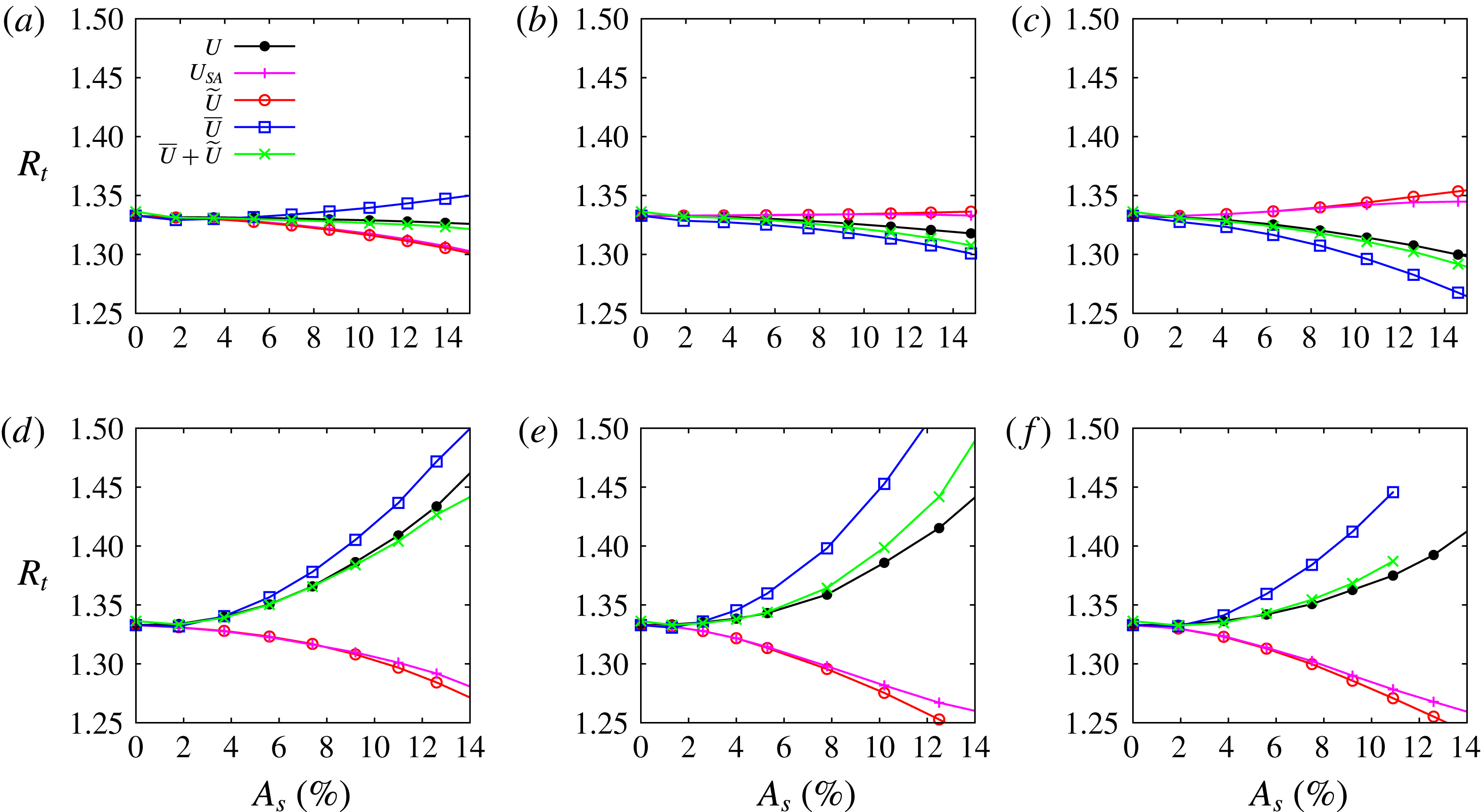
We find that, in all considered cases, the stability properties of the fictitious $\widetilde{U}$ profiles (red lines, open circles in figures 10 and 11) almost coincide with those obtained under the shape assumption (magenta lines with crosses). This means that the influences of higher spanwise-harmonics and of the change in shape of the first harmonic are negligible, and therefore not responsible for the qualitative differences between shape assumption and full nonlinear profiles results. On the contrary, the stability properties of the fictitious $\overline{U}$ profiles (blue lines, open squares in figures 10 and 11) are, in almost all considered cases, in qualitative (but often not in quantitative) agreement with the ones of the full nonlinear basic-flow profile (black lines with filled circles). This means that $\overline{\unicode[STIX]{x0394}U}(y)$ , despite its very small magnitude when compared to $\widetilde{\unicode[STIX]{x0394}U}$ ( $\max _{y}\overline{\unicode[STIX]{x0394}U}$ is at best $2\,\%$ or $3\,\%$ , depending on the streak symmetries when $A_{s}\approx 15\,\%$ ), has a stronger effect on the flow stability.

5.3 A composite second-order sensitivity

The results reported in the previous § 5.2, show that the (small amplitude) mean flow distortion $\overline{\unicode[STIX]{x0394}U}$ has the leading effect on the stability of the mixing layer while the (larger amplitude) spanwise-varying part of the nonlinear streaks $\widetilde{\unicode[STIX]{x0394}U}$ only mitigates or enhances this leading effect. These results must be reconciled with those of Hwang et al. (Reference Hwang, Kim and Choi2013) and Del Guercio et al. (Reference Del Guercio, Cossu and Pujals2014a ,Reference Del Guercio, Cossu and Pujals b ,Reference Del Guercio, Cossu and Pujals c ), where it was shown that the sensitivity of the growth rates on the streak amplitudes is quadratic, and with the second-order sensitivity analyses of Cossu (Reference Cossu2014), Tammisola et al. (Reference Tammisola, Giannetti, Citro and Juniper2014), Boujo et al. (Reference Boujo, Fani and Gallaire2015) and Tammisola (Reference Tammisola2017). The cornerstone of those analyses is that if the most unstable direct and adjoint modes of the 2D undisturbed basic flow are 2D (spanwise-uniform) and the basic-flow distortion $\widetilde{\unicode[STIX]{x0394}U}$ is spanwise sinusoidal then the first-order sensitivity of the leading growth rates to the 3D distortion amplitude (the streak amplitude $A_{s}$ ) is zero and the leading-order dependence is quadratic. However, we have just found that the leading effect on the stability of mixing layers is given by the spanwise-uniform mean flow distortion term $\overline{\unicode[STIX]{x0394}U}$ , which, therefore, has non-zero first-order sensitivity, apparently in contrast to the findings and/or the assumptions of those previous investigations.

The apparent paradox can, however, be removed by an analysis of the scaling of $\overline{\unicode[STIX]{x0394}U}$ . The equation for the evolution of $\overline{\unicode[STIX]{x0394}U}$ is easily obtained, under the (already made) assumptions that the reference basic flow has components $\{U(y),0,0\}$ and the perturbations are uniform in the streamwise direction, by averaging in the spanwise direction the streamwise component of (2.3):

(5.1) $$\begin{eqnarray}\frac{\unicode[STIX]{x2202}\unicode[STIX]{x0394}\overline{U}}{\unicode[STIX]{x2202}t}=-\frac{\unicode[STIX]{x2202}\overline{u^{\prime }v^{\prime }}}{\unicode[STIX]{x2202}y}+\frac{1}{Re}\frac{\unicode[STIX]{x2202}^{2}\unicode[STIX]{x0394}\overline{U}}{\unicode[STIX]{x2202}y^{2}}.\end{eqnarray}$$

Equation (5.1) is a standard Reynolds-averaged equation except for the fact that the average is performed in the spanwise direction, and not in time or the streamwise direction as usual. This equation clearly shows that $\overline{\unicode[STIX]{x0394}U}$ is generated by the Reynolds stress, which in our case is associated with the transient growth leading from the streamwise vortices to the streamwise streaks. If the viscous stress is neglected, which seems reasonable at the considered high $Re=1000$ , the amplitude of the mean flow distortion can therefore be expected to be proportional to the product of the characteristic amplitude of the vortices $A_{0}$ and that of the streaks $A_{s}$ . In the considered case, however, $A_{s}$ is almost proportional to $A_{0}$ (see figure 4), and therefore one can expect the mean flow distortion to scale proportionally to $A_{s}^{2}$ (or equivalently to $A_{0}^{2}$ ). This is verified to be indeed the case, as shown in figure 12, where the profiles $\unicode[STIX]{x0394}\overline{U}$ obtained for different amplitudes of the initial conditions for $\unicode[STIX]{x1D6FD}=2$ are virtually superposed and indistinguishable when rescaled by $A_{s}^{2}$ for both the optimal sinuous and the suboptimal varicose perturbations (similar results, not shown, are found for the other considered spanwise wavenumbers).

Figure 12.

Mean flow distortion rescaled by the square of the streaks amplitude $\overline{\unicode[STIX]{x0394}U}(y)/A_{s}^{2}$ corresponding to the forcing of the optimal sinuous (a) and suboptimal varicose (b) streaks with $\unicode[STIX]{x1D6FD}=2$ at $Re=1000$ . The profiles obtained for the three amplitudes $A_{s}\approx 5\,\%$ , $A_{s}\approx 10\,\%$ and $A_{s}\approx 15\,\%$ are reported in order to appreciate the accuracy of the scaling.

We are now ready to determine, in two steps, the leading-order modification (sensitivity) of the generic eigenvalue $\unicode[STIX]{x1D707}$ of the linear stability operator with respect to a modification $\unicode[STIX]{x0394}U=\overline{\unicode[STIX]{x0394}U}+\widetilde{\unicode[STIX]{x0394}U}$ (an equivalent but more systematic derivation is presented in appendix A). In the first step the reference basic flow is distorted only by the mean flow distortion $\overline{\unicode[STIX]{x0394}U}$ . As $\overline{\unicode[STIX]{x0394}U}$ is spanwise-uniform, the leading-order variation of $\unicode[STIX]{x1D707}$ depends, in general, linearly on the amplitude of $\overline{\unicode[STIX]{x0394}U}$ , and can be computed either by a linear fitting of the computed eigenvalues or explicitly, as detailed by Hill (Reference Hill1992), Chomaz (Reference Chomaz2005) and Giannetti & Luchini (Reference Giannetti and Luchini2007). As discussed above, however, the mean flow distortion is well approximated by $\overline{\unicode[STIX]{x0394}U}=A_{s}^{2}\overline{F}(y)$ , i.e. the amplitude of the mean flow distortion depends quadratically on the streak amplitude $A_{s}$ . At this stage, therefore, $\unicode[STIX]{x1D707}-\unicode[STIX]{x1D707}_{2D}\approx A_{s}^{2}\overline{\unicode[STIX]{x0394}\unicode[STIX]{x1D707}}$ . In the second step the (intermediate fictitious) 2D basic flow $\overline{U}=U_{2D}(y)+\overline{\unicode[STIX]{x0394}U}$ is distorted with the spanwise-periodic $\widetilde{\unicode[STIX]{x0394}U}$ to give the actual total distorted flow $U_{3D}(y,z)$ . In a first approximation $\widetilde{\unicode[STIX]{x0394}U}=A_{s}\widetilde{F}(y,z)$ if a shape assumption for the spanwise-periodic part of the distortion is made (this is justified by the discussion in § 5.2). As the distortion of the basic flow is now spanwise-periodic, the first-order sensitivity of $\unicode[STIX]{x1D707}$ to this distortion is zero and the leading-order term is the second-order term $A_{s}^{2}\widetilde{\unicode[STIX]{x0394}\unicode[STIX]{x1D707}}$ . The second-order sensitivity $\widetilde{\unicode[STIX]{x0394}\unicode[STIX]{x1D707}}$ can be computed by quadratic fitting of the computed eigenvalues or by an explicit second-order sensitivity analysis, as detailed by, for example, Tammisola et al. (Reference Tammisola, Giannetti, Citro and Juniper2014) and Boujo et al. (Reference Boujo, Fani and Gallaire2015). The combined result of the two-step asymptotic analysis is therefore that the eigenvalue $\unicode[STIX]{x1D707}$ of the linear stability operator pertaining to the streaky basic flow $U_{3D}(y,z)\approx U_{2D}(y)+\overline{\unicode[STIX]{x0394}U}(y)+\widetilde{\unicode[STIX]{x0394}U}(y,z)$ can, at leading order, be approximated by

(5.2) $$\begin{eqnarray}\unicode[STIX]{x1D707}-\unicode[STIX]{x1D707}_{2D}=A_{s}^{2}\widetilde{\unicode[STIX]{x0394}\unicode[STIX]{x1D707}}+A_{s}^{2}\overline{\unicode[STIX]{x0394}\unicode[STIX]{x1D707}},\end{eqnarray}$$

where $\unicode[STIX]{x1D707}_{2D}$ pertains to the (unperturbed) 2D profile, $\widetilde{\unicode[STIX]{x1D707}}$ is the second-order sensitivity to $A_{s}\widetilde{F}(y,z)$ , and $\overline{\unicode[STIX]{x1D707}}$ is the first-order sensitivity to $A_{s}^{2}\overline{F}(y)$ .

A qualitative assessment of the validity of (5.2) has been obtained by comparing, in figures 10 and 11, the value of $\unicode[STIX]{x1D707}$ given by the analysis of the full nonlinear $U_{3D}$ profile (black lines with filled circles) to $\unicode[STIX]{x1D707}_{2D}+A_{s}^{2}\widetilde{\unicode[STIX]{x0394}\unicode[STIX]{x1D707}}+A_{s}^{2}\overline{\unicode[STIX]{x0394}\unicode[STIX]{x1D707}}$ (green lines, $\times$ -symbols), where $A_{s}^{2}\widetilde{\unicode[STIX]{x0394}\unicode[STIX]{x1D707}}$ and $A_{s}^{2}\overline{\unicode[STIX]{x0394}\unicode[STIX]{x1D707}}$ are obtained from the analyses of the fictitious profiles $\overline{U}$ and $\widetilde{U}$ . From the figures it can be seen that the agreement is fairly good for small streak amplitudes ( $A_{s}\lesssim 6\,\%$ ) and, for all but two cases, acceptable even at quite higher streak amplitudes.

These results confirm that the variation of the eigenvalues remains quadratic at leading order even when the effects of the nonlinear mean flow distortion are taken into account. Taking into due account the mean flow distortion in sensitivity analyses, therefore, is not inconsistent with the quadratic variations of the eigenvalues with the streak amplitudes reported by Del Guercio et al. (Reference Del Guercio, Cossu and Pujals2014a ,Reference Del Guercio, Cossu and Pujals b ,Reference Del Guercio, Cossu and Pujals c ), who used the fully nonlinear streaks as basic flow.