1. Introduction
This work concerns the decay of magnetohydrodynamic turbulence in electrically conducting fluids subjected to an externally imposed magnetic field. We are particularly interested in the influence of solid, electrically insulating walls on this process. This generic problem is relevant to a number of practical engineering problems in the metallurgy and nuclear industry, but also bears relevance to some aspects of the dynamics of liquid planetary cores and the associated dynamo problem (even though, in this case the feedback of the flow onto the magnetic field introduces additional mechanisms not present at low magnetic Reynolds number,
 $Rm$
). Beyond MHD turbulence, the decay of strongly anisotropic turbulence can also reveal some of the mechanisms of the transition and competition between two- and three-dimensional turbulent dynamics, a process that is central in the geophysical context of e.g., atmospheric flows.
When the magnetic field
 $B\boldsymbol{e}_{z}$
is imposed (in the sense of the low magnetic Reynolds number approximation (Roberts Reference Roberts1967), turbulence evolves as a result of the competition between inertia and the diffusion of momentum along the direction of the magnetic field. A structure of size
 $l_{\bot }$
becomes elongated over a length
 $l_{z}$
by diffusion over a time scale of
 ${\it\tau}_{J}(l_{z}/l_{\bot })^{2}$
(Sommeria & Moreau Reference Sommeria and Moreau1982), whilst loosing energy through Joule dissipation (
 ${\it\tau}_{J}={\it\rho}/({\it\sigma}B^{2})$
is the Joule dissipation time,
 ${\it\rho}$
and
 ${\it\sigma}$
are the fluid density and electric conductivity). Moffatt (Reference Moffatt1967) first showed that under this linear phenomenology, the turbulent kinetic energy decayed at
 $E\sim (t/{\it\tau}_{J})^{-1/2}$
towards an asymptotic state where the flow quantities did not vary along the magnetic field (in this sense, a two-dimensional state) but where the kinetic energy of the component along the magnetic field was a third of the total kinetic energy (for a three-component flow). This phenomenology was recovered by Schumann (Reference Schumann1976): this author conducted low-resolution direct numerical simulations to confirm that this linear phenomenology applied during less than
 ${\it\tau}_{J}$
but that nonlinear effects subsequently led to a decay of the kinetic energy associated to the velocity along
 $\boldsymbol{B}$
. However, he also found that the skewness tended to a finite value in the later stages of the decay, which he attributed to the persistence of transport of kinetic energy along
 $\boldsymbol{B}$
. The more recent and higher resolution simulations of Burattini, Zikanov & Knaepen (Reference Burattini, Zikanov and Knaepen2010), Favier et al. (Reference Favier, Godeferd, Cambon and Delache2010, Reference Favier, Godeferd, Cambon, Delache and Bos2011), confirmed Schumann’s results and found a form of two-dimensional final state with greater energy in the transverse velocity components. Favier et al. (Reference Favier, Godeferd, Cambon and Delache2010) interpret this final state as two-and-a-half-dimensional (Shebalin, Matthaeus & Montgomery Reference Shebalin, Matthaeus and Montgomery1983), i.e., where the transverse component behave as in two-dimensional turbulence while the third component is advected as a passive scalar. Favier et al. (Reference Favier, Godeferd, Cambon, Delache and Bos2011) further showed that the discrepancy with the linear theory originated in the growth of anisotropy combining effects of linear Joule dissipation over time scale
 ${\it\tau}_{J}$
and much slower nonlinear effects. All three studies analysed cases where interaction parameter
 $N={\it\tau}_{U}/{\it\tau}_{J}$
spanned a range between 0.1 and 50 (
 ${\it\tau}_{U}(l_{0})=l_{0}/U(l_{0})$
is the eddy turnover time based on the initial size and velocity of the large scales
 $l_{0}$
and
 $U(l_{0})$
). Using the invariance of the ‘parallel’ component of Loitsyansky’s integral
 $I_{\Vert }$
, Okamoto, Davidson & Kaneda (Reference Okamoto, Davidson and Kaneda2010) showed that for
 $N\gg 1$
, the
 $(t/{\it\tau}_{J})^{-1/2}$
law for the decay of kinetic energy was recovered and that the integral length scale in the direction of the magnetic field evolved as
 $l_{z}\sim (t/{\it\tau}_{j})^{1/2}$
. At moderate values of
 $N$
, a similar approach led the authors to conclude that energy decayed as
 $E\sim (t/{\it\tau}_{J})^{-11/7}$
while the integral length scales along and across the magnetic field increased respectively as
 $l_{z}\sim (t/{\it\tau}_{J})^{5/7}$
and
 $l_{\bot }\sim (t/{\it\tau}_{J})^{3/14}$
. These theoretical scalings as well as the invariance of
 $I_{\Vert }$
were verified by means of direct numerical simulations at the highest resolution available to date (up to
 $2048^{3}$
), for
 $N<1$
. Since the flow tends towards a two-dimensional state, boundaries perpendicular to the magnetic field always play an important role in the dynamics in a number of realistic situations. Hence without realistic (and computationally costly) boundary conditions, the latest stages of the decay could not be analysed up to now, leaving open the question of the state that MHD turbulence ultimately decays to. The presence of realistic Hartmann walls (perpendicular to the magnetic field) adds an important element to the problem of turbulent decay for three reasons.
-
(1) In the presence of solid walls, turbulence can reach a physically realistic quasi-two-dimensional state. The main question concerning the later stages of the decay becomes to find to which extent quasi-two-dimensionality is achieved.
-
(2) Turbulence between Hartmann walls can be reproduced experimentally (for example using the FLOWCUBE platform (Klein & Pothérat Reference Klein and Pothérat2010; Pothérat & Klein Reference Pothérat and Klein2014)) so (1) can be answered both numerically and experimentally.
-
(3) In decaying turbulence, physical mechanisms can be more easily be identified through their characteristic time scales than in forced turbulence in a statistically steady state. Hence decaying turbulence between walls provides an insight into the mechanisms at play in wall-bounded MHD turbulence too.
In this type of turbulence, a strictly two-dimensional state is not possible because of the very thin Hartmann boundary layers that develop along them (see for instance Moreau Reference Moreau1990). Instead, Sommeria & Moreau (Reference Sommeria and Moreau1982) theorised that in a channel of width
 $L$
, a structure of size
 $l_{\bot }$
became quasi-two-dimensional after
 ${\it\tau}_{2D}(l_{\bot })\sim {\it\tau}_{J}(L/l_{\bot })^{2}$
. Past this stage, electric current in the core became of order
 $Ha^{-1}$
, the ratio of the boundary-layer thickness to
 $L$
: dissipation occurred then almost exclusively in the boundary layers and was equally viscous and magnetic. In contrast, strictly two-dimensional states are possible when walls are absent and the Joule dissipation can therefore drop to much lower values. Kolesnikov & Tsinober (Reference Kolesnikov and Tsinober1974) also observed experimentally that in the presence of Hartmann walls, transport along the magnetic field was suppressed in the later stages of the decay. This was interpreted as an evidence of suppression of the velocity component in this direction, in contrast to the prediction of theories and simulations where no wall was present. Nevertheless, although a ‘through’ velocity component is precluded by the walls, Ekman pumping can still potentially lead to strong wall-normal velocities at moderate
 $N$
(Pothérat, Sommeria & Moreau Reference Pothérat, Sommeria and Moreau2000). More recently, it was also found that even for
 $N>1$
, a small amount of three-dimensionality could lead to a complex system of three-dimensional co- and contrarotating recirculations (Pothérat et al.
Reference Pothérat, Rubiconi, Charles and Dousset2013; Baker, Pothérat & Davoust Reference Baker, Pothérat and Davoust2015).
Until recently, numerically simulating MHD turbulence at high
 $N$
in the presence of walls incurred prohibitive computational costs because of the need to resolve the Hartmann boundary layers. Recently, the authors took a different approach to the simulation of these flows based on spectral methods using bases of functions whose elements already incorporate these layers. These partly alleviate this computational constraint to the point where the computational cost becomes independent of
 $Ha$
(Dymkou & Pothérat Reference Dymkou and Pothérat2009; Kornet & Pothérat Reference Kornet and Pothérat2015). We propose to take advantage of this new technique to investigate decaying turbulence in a channel bounded by electrically insulating walls in view of answering the following questions.
-
(1) Does three-dimensionality subsist in the later stages of the decay (
 $t\gg {\it\tau}_{2D}(l_{0})$
)?
-
(2) How much energy subsists in the third velocity component?
-
(3) How do Hartmann walls affect the early phases of the decay (
$t<{\it\tau}_{2D}(l_{0})$
)?


We shall first recall the governing equations and the time scales that govern the problem (§ 2). Numerical methods and simulation strategy are presented in § 3. After an overview of the decay (§ 4), we examine the earlier decay phase which is expected to present the strongest similarities with earlier works not involving walls (§ 5). The later stages of the decay where similarities with two-dimensional turbulence are expected are analysed in § 6. The robustness of our results is tested in § 7 by changing initial conditions and domain size.
2. Governing equations
2.1. Problem definition
At low magnetic Reynolds number, the full system of the induction equation and the Navier–Stokes equations for an incompressible fluid can be approximated to the first order (the magnetic Reynolds number
 $Rm$
represents the ratio of the induced magnetic field to the imposed one). This leads to the following system (Roberts Reference Roberts1967):
 $$\begin{eqnarray}\displaystyle & \displaystyle \frac{\partial \boldsymbol{u}}{\partial t}+(\boldsymbol{u}\boldsymbol{\cdot }\boldsymbol{{\rm\nabla}})\boldsymbol{u}=-\frac{1}{{\it\rho}}\boldsymbol{{\rm\nabla}}p+{\it\nu}{\rm\Delta}\boldsymbol{u}+\frac{1}{{\it\rho}}\boldsymbol{j}\times \boldsymbol{B}, & \displaystyle\end{eqnarray}$$
 $$\begin{eqnarray}\displaystyle & \displaystyle \boldsymbol{{\rm\nabla}}\boldsymbol{\cdot }\boldsymbol{u}=0, & \displaystyle\end{eqnarray}$$
 $$\begin{eqnarray}\displaystyle & \displaystyle \boldsymbol{{\rm\nabla}}\boldsymbol{\cdot }\boldsymbol{j}=0, & \displaystyle\end{eqnarray}$$
 $$\begin{eqnarray}\displaystyle & \displaystyle \boldsymbol{j}={\it\sigma}(-\boldsymbol{{\rm\nabla}}{\it\Phi}+\boldsymbol{u}\times \boldsymbol{B}), & \displaystyle\end{eqnarray}$$
 $\boldsymbol{u}$
denotes the fluid velocity,
 $\boldsymbol{B}$
the externally imposed magnetic field,
 $\boldsymbol{j}$
the electric current density,
 ${\it\nu}$
the kinematic viscosity,
 ${\it\sigma}$
the electrical conductivity, and
 ${\it\Phi}$
the electric potential.
The validity of the quasi-static, low-
 $Rm$
approximation is widely accepted for configurations corresponding to small-scale laboratory experiments involving liquid metals flows of moderate intensity. Scale and flow intensity indeed guarantee that
 $Rm\ll 1$
but not necessarily that the unsteady term in the induction equations (which is responsible for the presence of Alfvén waves (Roberts Reference Roberts1967)), is negligible compared to magnetic diffusion. The ratio of these two effects is controlled by the Lundquist number
 $S=HaP_{m}^{1/2}$
. For sufficiently high Hartmann numbers, and depending on the value of the magnetic Prandtl number
 $P_{m}$
, the quasi-static assumption could be challenged. In liquid metals,
 $P_{m}$
lies in the range
 $10^{-6}{-}10^{-5}$
so that the quasi-static approximation holds up to
 $Ha\sim 10^{3}$
. Recent MHD experiments now involve transparent electrolytes, which, despite their low electric conductivity make direct flow optical visualisation accessible with the shadograph technique (Andreev, Kolesnikov & Thess Reference Andreev, Kolesnikov and Thess2006) or particle image velocimetry (Andreev, Kolesnikov & Thess Reference Andreev, Kolesnikov and Thess2013). For electrolytes,
 $P_{m}\sim 10^{-9}$
, so the quasi-static approximation would hold up to
 $Ha\sim 10^{5}$
. To reach such values, however, the very low electrical conductivity of electrolytes (
 $10^{4}$
times lower than liquid metals, typically), would require very large experiments in extremely high magnetic fields. With electrolytes (Sulfuric acid for example) in the largest magnets currently available,
 $Ha$
cannot exceed
 ${\sim}10^{3}$
. In the light of this discussion, simulations in the present work shall be restricted to
 $Ha<10^{3}$
, where the quasi-static approximation holds both for liquid metals and electrolytes, with laboratory experiments in mind.
The geometry of the problem is that of a channel flow with a homogeneous transverse magnetic field
 $B\boldsymbol{e}_{z}$
and impermeable (
 $\boldsymbol{u}|_{wall}=\mathbf{0}$
), electrically insulating (
 $\boldsymbol{j}\boldsymbol{\cdot }\boldsymbol{n}|_{wall}=\mathbf{0}$
) walls located at
 $z=\pm L/2$
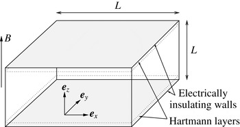
(see figure 1). Periodic boundary conditions of period
 $L$
are imposed in the
 $x$
and
 $y$
directions. Following Sommeria & Moreau (Reference Sommeria and Moreau1982), the Lorentz force can be expressed as the sum of a gradient of magnetic pressure
 $p_{m}$
and a rotational term:
 $$\begin{eqnarray}\boldsymbol{j}\times \boldsymbol{B}=-\frac{\boldsymbol{{\rm\nabla}}p_{m}}{{\it\rho}}-{\it\sigma}B^{2}{\it\Delta}^{-1}\partial _{zz}\boldsymbol{u}.\end{eqnarray}$$
Using the above identity and adopting reference scale
 $L$
, time
 $L^{2}/{\it\nu}$
and velocity
 ${\it\nu}/L$
, the set of (2.1)–(2.4) can be expressed in dimensionless form:
 $$\begin{eqnarray}\frac{\partial \boldsymbol{u}}{\partial t}+P[(\boldsymbol{u}\boldsymbol{\cdot }\boldsymbol{{\rm\nabla}})\boldsymbol{u}]={\rm\Delta}\boldsymbol{u}-\frac{1}{Ha^{2}}{\it\Delta}^{-1}\partial _{zz}\boldsymbol{u},\end{eqnarray}$$
where
 $Ha=LB\sqrt{{\it\sigma}/{\it\rho}{\it\nu}}$
is the Hartman number and
 $P$
denotes orthogonal projection onto the subspace of solenoidal fields.
Geometry of the channel flow with transverse magnetic field.

2.2. Time scales of the decay
Consider now an initially turbulent, isotropic flow, left to decay from
 $t=0$
under the action of the Lorentz force and viscous friction, in the configuration described above. Hartmann walls can be expected to exert little influence on the initial phase of the decay, during which strong two-dimensionalisation of the flow should take place, as in the simulations of Schumann (Reference Schumann1976), Okamoto et al. (Reference Okamoto, Davidson and Kaneda2010) and others. Unlike, in these previous studies, the presence of physical walls may lead to a physically realistic phase beyond this initial one, where the flow dynamics may become two-dimensional to some extent. To obtain a first estimate for the time scale for the transition between these two phases, let us first consider a single turbulent structure of size
 $l_{\bot }$
, which diffuses across the channel width
 $L$
under the action of the Lorentz force in time
 ${\it\tau}_{2D}(l_{\bot })={\it\tau}_{J}(L/l_{\bot })^{2}$
. If this time scale is shorter than both the inertial time scale
 ${\it\tau}_{U}(l_{\bot })=l_{\bot }/U(l_{\bot })$
and the viscous time scale
 ${\it\tau}_{{\it\nu}}(l_{\bot })=l_{\bot }^{2}/{\it\nu}$
, then this single structure is quasi-two-dimensional. Two conditions for two-dimensionality ensue:
 $$\begin{eqnarray}\displaystyle & \displaystyle \left(\frac{l_{\bot }}{L}\right)^{3}>\frac{l_{0}}{L}\frac{U(l_{\bot })}{U(l_{0})}\frac{1}{N(l_{0})}, & \displaystyle\end{eqnarray}$$
 $$\begin{eqnarray}\displaystyle & \displaystyle \left(\frac{l_{\bot }}{L}\right)^{2}>\frac{1}{Ha}, & \displaystyle\end{eqnarray}$$
 $l_{0}$
denotes the size of the large scales at
 $t=0$
. Each these conditions defines a minimum two-dimensional scale. Consequently, in a turbulent flow where
 $N={\it\tau}_{U}(l_{\bot })/{\it\tau}_{J}\gg 1$
, larger scales are two-dimensional while smaller scales may still be three-dimensional. From inertial condition (2.7), the smallest quasi-two-dimensional structure satisfies
 $l_{\bot }^{2D}\sim L[(l_{0}U(l_{\bot }^{2D}))/(N(l_{0})LU(l_{0}))]^{1/3}$
. Since the two-dimensionalisation time
 ${\it\tau}_{2D}(l_{\bot })$
increases with
 $l_{\bot }$
, this scale is also the slowest structure to become two-dimensional and so
 ${\it\tau}_{2D}^{M}={\it\tau}_{2D}(l_{\bot }^{2D})$
provides an estimate for the two-dimensionalisation phase:
 $$\begin{eqnarray}{\it\tau}_{2D}^{M}\sim {\it\tau}_{J}\left(N(l_{0})\frac{U(l_{0})L}{U(l_{\bot }^{2D})l_{0}}\right)^{2/3}.\end{eqnarray}$$
 ${\it\tau}_{2D}^{M}$
depends on
 $U(l_{\bot }^{2D})$
, which is expected to drop by several orders of magnitudes during the two-dimensionalisation phase. Not only does this variation of
 $U(l_{\bot }^{2D})$
considerably slow down two-dimensionalisation at the initial scale
 $l_{\bot }^{2D}(t=0)$
, but scales smaller than the initial value of
 $l_{\bot }^{2D}$
may satisfy (2.7) and may in turn become quasi-two-dimensional in a time scale significantly longer than the initial value of (2.9). On these grounds, a lower estimate for the two-dimensionalisation time is obtained by evaluating (2.9) based on the value of
 $U(l_{\bot })$
at
 $t=0$
(this value is fixed by the choice of initial turbulent spectrum).
From viscous condition (2.8), by contrast, the smallest quasi-two-dimensional scale
 $l_{\bot }^{2D}$
does not depend on
 $U(l_{\bot })$
, and neither does the associated two-dimensionalisation time:
 $$\begin{eqnarray}\displaystyle & \displaystyle l_{\bot }^{2D}\sim LHa^{-1/2}, & \displaystyle\end{eqnarray}$$
 $$\begin{eqnarray}\displaystyle & \displaystyle {\it\tau}_{2D}^{M}={\it\tau}_{2D}(l_{\bot }^{2D})\sim {\it\tau}_{J}Ha^{-1}={\it\tau}_{H}. & \displaystyle\end{eqnarray}$$
 ${\it\tau}_{H}$
represents a closer estimate of the time scale for two-dimensionalisation of the whole turbulent flow than (2.9).
2.3. Two-dimensional decay
Once all structures have become quasi two-dimensional, the evolution of the flow is governed by two-dimensional dynamics with an added friction due to the Hartmann layers. Sommeria & Moreau (Reference Sommeria and Moreau1982) showed that the velocity averaged across the channel
 $\bar{\boldsymbol{u}}=\int _{-1}^{1}\boldsymbol{u}_{\bot }\,\text{d}z$
satisfied a shallow water equation of the form:
 $$\begin{eqnarray}\displaystyle & \displaystyle \frac{\partial \bar{\boldsymbol{u}}}{\partial t}+(\bar{\boldsymbol{u}}\boldsymbol{\cdot }\boldsymbol{{\rm\nabla}}_{\bot })\bar{\boldsymbol{u}}=-\frac{1}{{\it\rho}}\boldsymbol{{\rm\nabla}}_{\bot }p+{\it\nu}{\it\Delta}_{\bot }\bar{\boldsymbol{u}}-\frac{2\bar{\boldsymbol{u}}}{{\it\tau}_{H}}, & \displaystyle\end{eqnarray}$$
 $$\begin{eqnarray}\displaystyle & \displaystyle \boldsymbol{{\rm\nabla}}_{\bot }\boldsymbol{\cdot }\bar{\boldsymbol{u}}=0, & \displaystyle\end{eqnarray}$$
 $\bot$
operate in the
 $x$
–
 $y$
plane only.
 ${\it\tau}_{H}$
appears as the typical time for the dissipation due to the Hartmann boundary layers, and therefore a characteristic time of the two-dimensional dynamics. Integrating
 $\bar{\boldsymbol{u}}~\boldsymbol{\cdot }$
(2.12) over the fluid domain, the evolution of the total kinetic energy
 $E\simeq E_{2D}=\Vert \bar{\boldsymbol{u}}\Vert _{2}^{2}$
associated to the mean flow
 $\bar{\boldsymbol{u}}$
when the flow follows a two-dimensional dynamics reduces to
 $$\begin{eqnarray}\frac{1}{2}\frac{\text{d}E_{2D}}{\text{d}t}=-2\frac{E_{2D}}{{\it\tau}_{H}}-{\it\nu}\Vert \boldsymbol{{\rm\nabla}}\bar{\boldsymbol{u}}\Vert _{2D}^{2},\end{eqnarray}$$
where
 $\Vert \cdot \Vert _{2D}$
represents the two-dimensional
 $\mathscr{L}^{2}$
norm. Introducing length scale
 $l_{\bot }^{{\it\nu}}=(\Vert \bar{\boldsymbol{u}}\Vert _{2D}^{2}/\Vert \boldsymbol{{\rm\nabla}}\bar{\boldsymbol{u}}\Vert _{2D}^{2})^{1/2}$
which characterises velocity gradients in the
 $(x,y)$
plane, then
 $$\begin{eqnarray}\frac{\text{d}E_{2D}}{\text{d}t}=-\frac{4}{{\it\tau}_{H}}\left[1+\frac{1}{2Ha}\left(\frac{L}{l_{\bot }^{{\it\nu}}}\right)^{2}\right]E_{2D}.\end{eqnarray}$$
It follows from the respective definitions of the total kinetic energy
 $E$
and
 $E_{2D}$
, that
 $$\begin{eqnarray}E=E_{2D}(1+\mathit{O}(\max \{Ha^{-1},{\it\alpha}^{2}\})),\end{eqnarray}$$
where
 ${\it\alpha}=\Vert \boldsymbol{u}-\bar{\boldsymbol{u}}\Vert /\Vert \boldsymbol{u}\Vert$
represents the degree of three-dimensionality in the flow. For a quasi-two-dimensional flow,
 $E=E_{2D}(1+\mathit{O}(Ha^{-1}))$
. We shall see from the analysis of flow profiles in § 6 (figure 9) that in the later stages of the decay,
 ${\it\alpha}\lesssim 0.1$
, so
 $E_{2D}$
can be expected to provide a good approximation for
 $E$
in the two-dimensional phase of the decay.
The two-dimensional dynamics of the flow is expected to favour the formation of large scales and indeed Schumann (Reference Schumann1976) and Favier et al. (Reference Favier, Godeferd, Cambon and Delache2010) showed that energy transfer towards them occurred during the decay. Areas of strong shear may however persist between them. Furthermore, the typical length scale of the viscous core of quasi-two-dimensional MHD vortices is known to scale as
 $LHa^{-1/2}$
(Sommeria Reference Sommeria1988). For such fine quasi-two dimensional structures, Hartmann friction and horizontal viscous friction would be of the same order. For large structures however,
 $l_{\bot }^{{\it\nu}}/L$
should be of the order of unity and so in the limit
 $Ha\rightarrow \infty$
, the decay should be strongly dominated by Hartmann friction. The total kinetic energy should then decay as
 $E\sim \exp (-4t/{\it\tau}_{H})$
. Any discrepancy to exponential decay of this form is therefore the signature either of thin quasi-two-dimensional structures or of a residual three-dimensionality. We shall attempt to measure this discrepancy in our numerical simulation to identify the mechanisms of the long-term decay in § 6.3. It should, however, be noted that for structures such that
 $l_{\bot }^{{\it\nu}}/L\sim Ha^{-1/2}$
, three-dimensionality subsists anyway because at this scale, friction between horizontal planes balances the diffusion of momentum along the magnetic field.
3. Numerical approach
3.1. Numerical method
The problem set out in § 2.1 is solved numerically, using a new type of spectral method designed to alleviate the computational cost associated with strong anisotropy and thin Hartmann boundary layers. The main idea is to take advantage of the fact that such structures are dissipative and that their presence should reduce the number of degrees of freedom of the flow, when paradoxically, their fine resolution incurs extra computational cost in most current methods. The mathematical principle is to use a functional basis with elements that already include these fine structures so as to avoid these extra costs. The main advantage of this technique is that Hartmann layers are finely resolved with a limited number of collocation points, so in contrast to traditional methods, the computational cost per time step does not depend on the intensity of the magnetic field. This makes it possible to simulate flows at much higher magnetic fields than standard methods (such as spectral methods based on Techbychev polynomials, which break down when the high resolution required to solve either turbulence or the Hartmann layers leads to ill-conditioned problems). Another advantage of this technique is that it can potentially be adapted to a number of other problems where fine resolution becomes problematic in extreme regimes, as long as a suitable basis can be found either analytically or numerically. This step may however prove tedious, even for a simple change in boundary conditions (see for instance Low & Pothérat (Reference Low and Pothérat2015) for the case of an MHD channel with parallel magnetic field). The mathematical foundations of this method and its numerical implementation are described in detail in Dymkou & Pothérat (Reference Dymkou and Pothérat2009), Kornet & Pothérat (Reference Kornet and Pothérat2015), where it is also tested for the exact channel geometry studied here. For the sake of completeness, we shall nevertheless outline the principle of this new method. Using the spectral approach we seek the solution of (2.6) as the decomposition on elements of basis
 $\boldsymbol{u}_{i}$
:
 $$\begin{eqnarray}\boldsymbol{u}=\mathop{\sum }_{i}c_{i}(t)\boldsymbol{u}_{i}(\boldsymbol{x}).\end{eqnarray}$$
As the spatial dependence is carried solely by
 $\boldsymbol{u}_{i}$
, when representation (3.1) is injected into (2.6), the latter reduces to the set of ordinary differential equations in time on the unknown coefficients
 $c_{i}(t)$
(see Canuto et al. (Reference Canuto, Hussaini, Quarteroni and Zang2006) for a detailed description of spectral methods).
For the basis
 $\boldsymbol{u}_{i}$
we choose the set of eigenfunctions of the operator
 $\mathscr{L}$
formally expressed as the right-hand side of (2.6), with the electrical and kinematic boundary conditions of the problem. These functions are a natural choice as elements of a functional basis because the features of flows at high
 $Ha$
are strongly determined by the properties of this operator. For example, they include specific features of the flow such as laminar and turbulent Hartmann boundary layers that develop along the channel walls (Dymkou & Pothérat Reference Dymkou and Pothérat2009; Pothérat & Dymkou Reference Pothérat and Dymkou2010). Moreover, these modes all have negative eigenvalues, and it can be shown that to resolve the flow completely, it is only necessary to take into account all modes with eigenvalue
 ${\it\lambda}$
of modulus below a maximum
 $|{\it\lambda}_{max}|$
, such that their total number scales as
 $Re^{2}/Ha$
(Pothérat & Alboussière Reference Pothérat and Alboussière2006), where
 $Re$
is the Reynolds number based on the large scales. Since the operator
 $\mathscr{L}$
represents the sum of viscous and ohmic dissipation, the set of modes defined in this way is in fact the set of least dissipative modes.
The main difficulty in solving (2.6) using the least dissipative modes lies in calculating the spectral representation of the nonlinear terms
 $G(\boldsymbol{u}(x_{i},y_{i},z_{i}))$
. We use a pseudospectral approach and calculate these terms in real space. Therefore we need a method to reconstruct the spectral coefficients
 $g_{n}$
of physical vector fields known at a discrete set of points in space
 $x_{i}$
. To this aim, we first use the fact that the eigenmodes of
 $\mathscr{L}$
can be factorised as the product of two scalar functions of
 $x$
and
 $y$
, respectively, and a vector function of
 $z$
. Moreover, the functions of
 $x$
and
 $y$
consist of Fourier modes, so the set of eigenmodes can be enumerated by a tuple of three numbers
 $(n_{x},n_{y},n_{z})$
and for every mode we can define the vector function
 $\boldsymbol{E}_{n_{x},n_{y},n_{z}}(z)$
such that each mode takes the form
 $$\begin{eqnarray}\boldsymbol{E}_{n_{x},n_{y},n_{z}}(z)\exp (\text{i}k_{n_{x}}x+\text{i}k_{n_{y}}y).\end{eqnarray}$$
Therefore we first calculate the two-dimensional fast Fourier transform in the
 $x$
–
 $y$
directions. This brings the transformed nonlinear terms under the form:
 $$\begin{eqnarray}G(\boldsymbol{u}(x_{i},y_{i},z_{i}))=\mathop{\sum }_{n_{x},n_{y}}\boldsymbol{A}_{n_{x},n_{y}}(z_{i})\exp (\text{i}2{\rm\pi}n_{x}x_{i}+\text{i}2{\rm\pi}n_{y}y_{i}),\end{eqnarray}$$
where
 $\boldsymbol{A}_{n_{x},n_{y}}$
is the complex amplitude of Fourier mode
 $(2{\rm\pi}n_{x},2{\rm\pi}n_{y})$
. Then, for every value of
 $(n_{x},n_{y})$
we find the set of spectral coefficients
 $\{g_{n_{x},n_{y},n_{z}}\}$
by solving a set of equations
 $$\begin{eqnarray}\mathop{\sum }_{n_{z}}g_{n_{x},n_{y},n_{z}}\boldsymbol{E}_{n_{x}n_{y}n_{z}}(z_{i})=\boldsymbol{A}_{n_{x},n_{y}}(z_{i}).\end{eqnarray}$$
As the coefficients in this set of equations are constant during a single numerical run, it is worth performing the
 $LU$
decomposition of the corresponding matrix at the beginning of calculations and later use it to efficiently find the spectral decompositions. Finally, the projection onto the subspace of solenoidal vector fields is performed by neglecting the coefficients corresponding to modes with non-zero divergence. Using the Fast Fourier transform in
 $x{-}y$
planes imposes the distribution of discretisation points in these planes: they have to form a regular rectangular grid. We denote its dimensions as
 $N_{x}\times N_{y}$
. The method described so far does not a priori constrain the distribution of points in
 $z$
direction. However our tests indicate that if the density of points is higher in the vicinity of the walls than in the midplane, the set of (3.4) tends to become more ill conditioned, and this affects numerical precision. Furthermore, the resolution of the small scales of turbulence in the initial phases of the decay requires a high resolution in the core. A uniform grid in the
 $z$
direction (with
 $N_{z}$
points) is therefore best suited to resolve turbulence whilst minimising error. For the set of (3.4) to have a unique solution, the number of modes used during the spectral decomposition has to be equal to
 $N_{z}$
, and the total number of independent modes used in the calculations is
 $N=N_{x}N_{y}N_{z}$
. The technique described above has the advantage that the obtained spectral decomposition reproduces exactly the physical field on the given set of discretisation points. Therefore momentum and energy are conserved by this procedure. However the spectral coefficients
 $g_{n}$
obtained in this way are different from the exact ones
 $\widetilde{g}_{n}$
, that would be obtained by decomposition of the same vector field over the space of infinite dimension spanned by all eigenvectors of
 $\mathscr{L}\cdot |\widetilde{g}_{n}-g_{n}|$
is the so-called aliasing error. To correct this error we adapt the
 $3/2$
technique known from standard spectral methods (Canuto et al.
Reference Canuto, Hussaini, Quarteroni and Zang2006). Namely we perform the discrete transformation with additional number of modes
 $N$
larger than the one strictly required by the system’s dynamics,
 $N_{D}$
(the latter is of the order of the attractor dimension of the dynamical system underlying the given problem (Pothérat & Alboussière Reference Pothérat and Alboussière2006)). After every evaluation of the spectral decomposition, the coefficients corresponding to these additional modes are set to zero.
The spectral method described above was implemented by modifying the spectral code TARANG developed by Verma et al. (Reference Verma, Chatterjee, Reddy, Yadav, Paul, Chandra and Samtaney2013).
3.2. Simulation strategy
The bulk of our numerical simulations was based on a domain made of a cube of dimension
 $L$
divided uniformly into
 $N_{x}$
,
 $N_{y}$
and
 $N_{z}$
cells respectively in
 $x$
,
 $y$
and
 $z$
directions. Our previous studies (Kornet & Pothérat Reference Kornet and Pothérat2015) showed that to keep the dealiasing errors under control it is sufficient to resolve each of the Hartmann layers with three computational cells. The ability of our method to precisely resolve Hartmann layers with a relatively coarse grid is a clear benefit of the choice of spectral basis that already incorporates Hartmann layers. Furthermore, unlike previous studies of MHD turbulence with periodic boundary conditions, domain boundaries perpendicular to the magnetic field are physical walls that actively participate in the physics of the flow. It is therefore not desirable to increase the size of the domain in the magnetic field direction, unlike in these studies, where periodic boundary conditions introduced unphysical artefacts (see e.g., Vorobev et al.
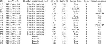
Reference Vorobev, Zikanov, Davidson and Knaepen2005). Our strategy to study the decay of MHD turbulence relies on four different types of simulations, all gathered in table 1.
Summary of parameters of calculated 3-D cases.

The first type is inspired from the DNS of decaying MHD turbulence in a three-dimensional periodic domain by Okamoto et al. (Reference Okamoto, Davidson and Kaneda2010): the initial conditions consist of a isotropic, random Gaussian velocity field with
 $u(k)\sim \exp [(-k/k_{p})^{2}]$
where
 $k_{p}=4{\rm\pi}/L$
. This corresponds to an energy spectrum
 $E\sim k^{4}\exp [-2(k/k_{p})^{2}]$
. For this choice of initial velocity field, the initial integral scale of turbulent motion is given by
 $l_{0}=\sqrt{2{\rm\pi}}/k_{p}$
. The velocity spectrum was normalised in such a way that cell sizes in
 $x$
and
 $y$
directions correspond to
 $l_{K}/1.4$
, where
 $l_{K}=l_{0}Re^{-3/4}$
is the Kolmogorov length scale and the Reynolds number in its definition
 $Re=u^{\prime }l/{\it\nu}$
is based on
 $l$
and velocity
 $u^{\prime }=u~(k=k_{p})$
. This strategy allows us to calculate the most intense flow possible whilst minimising mesh-induced numerical errors at a given mesh size, since the mesh is always uniform. The initial velocity field was first generated in the Fourier space and evaluated at every point of the computational domain. The resulting field was then projected onto the functional basis of least dissipative modes. This resulted in a steep drop of velocities at points located within the Hartmann layers, since all elements of the functional basis satisfy no-slip, impermeable boundary conditions.
To characterise the influence of the walls, we performed additional simulations starting from exactly the same initial conditions as before, but with periodic boundary conditions imposed in all three directions. For this set of calculations we used a traditional spectral code, Turbo, which uses Fourier modes as the functional basis and was tested and optimised for Low-
 $Rm$
MHD (Knaepen & Moin Reference Knaepen and Moin2004; Vorobev et al.
Reference Vorobev, Zikanov, Davidson and Knaepen2005).
To evaluate a possible influence of the size of the domain in the
 $x$
and
 $y$
dimensions, we also performed several simulations with a domain of dimension
 $2L$
in these directions. These were computationally expensive and therefore run over a shorter period of time than the simulation over a cube of size
 $L$
.
Finally, the simple order of magnitude analysis from § 2.2 shows that under a strong magnetic field, the decay of MHD turbulence can occurs over a time of the order of a few times
 ${\it\tau}_{J}$
, while a truly quasi-two-dimensional behaviour would not be expected before smaller scales are diffused over the height of the channel, i.e., at much later times, of the order of
 ${\it\tau}_{H}=Ha{\it\tau}_{J}$
. Thus, if the initial integral scale
 $l_{0}$
is chosen much smaller than the size of the box, turbulence will have lost practically all of its kinetic energy by the time the two-dimensional dynamics potentially becomes dominant. This would make it difficult to study the later phase of the decay. However,
 $l_{0}/L$
needs to be sufficiently smaller than unity for a significant three-dimensional phase of the decay to exist and so as to generate a sensible transition between three- and two-dimensional dynamics. To reconcile these antagonistic constraints, we chose
 $l_{0}/L=1/\sqrt{(2{\rm\pi})}\simeq 0.4$
and also run additional simulations initialised with the velocity field obtained at
 $t=0.5{\it\tau}_{J},{\it\tau}_{J}$
in the previous simulations, but in which the velocities are renormalised, so that the total energy is restored to its level at
 $t=0$
(these are referred to as ‘boosted’ in table 1. Renormalisation is applied only once at the time specified in the table for each case, and the flow is left to decay freely again after this time). The flow obtained this way is much closer to a quasi-two-dimensional one than the simulations initialised with a random field. In the same spirit, two further simulations were performed with a quasi-two-dimensional initial flow (thereafter denoted ‘2-D’ in figure legends). The initialization procedure follows that applied to three-dimensional initial conditions, except that during generation of velocity field in Fourier space we remove all modes with
 $k_{z}\neq 0$
and then renormalise the flow in such a way that the total kinetic energy be equal to
 $2/3$
of the kinetic energy of the corresponding with 3-D initial conditions. Comparing the evolutions of these different types of initial conditions shall thus give us a good measure of the robustness of the features observed in the later stages of the decay to a change of initial conditions and to the intensity of the initial flow.
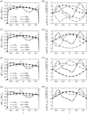
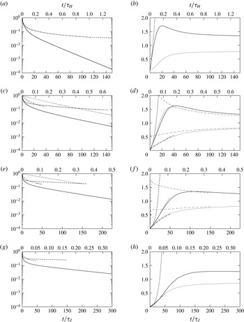
(a,c,e,g) Evolution of the normalised, spatial RMS of all vertical profiles of
 $\langle \boldsymbol{u}_{\bot }^{2}\rangle$
over all
 $(x,y)$
in the domain. (b,d,f,h) Evolution of
 $u_{z}$
along a vertical line in the middle of the domain. In all cases, the initial flow was homogenous and 3-D isotropic away from the walls; (a,b)
 $Ha=112$
; (c,d)
 $Ha=224$
; (e,f)
 $Ha=448$
; (g,h)
 $Ha=896$
.

3.3. Computing times
At
 $Ha=112$
, the computing time per time step for cases with walls is about four times higher than that with periodic boundary conditions (the latter featuring a lower resolution). As theoretically predicted (Kornet & Pothérat Reference Kornet and Pothérat2015), this cost remains constant when
 $Ha$
is increased, which is a major benefit of our method over traditional spectral methods based on Tchebychev polynomials. Since the number of time steps per Joule time is essentially independent of
 $Ha$
too, all calculations with walls take approximately the same time. These were performed on 100 cores of a cluster built on two-processor nodes using Intel Xeon Nehelem 2.4 GHz, for which calculations of
 $150{\it\tau}_{J}$
took approximately 20 days.
4. General evolution of the flow
Consider first the decay of initially isotropic turbulence in the domains of size
 $L^{3}$
. From the evolution of the total energy (figure 6), the flow progresses in every case through three consecutive phases: during the first phase, the flow adjusts from the initial conditions. This phase is very short, (shorter than
 $0.05{\it\tau}_{J}$
in all cases). A second phase immediately follows, where strongly three-dimensional turbulence is present with erratic flow in all directions. This phase can be identified through the strong three-dimensionality visible in the spatial RMS for all
 $(x,y)$
of the profile along
 $z$
of magnitude of
 $\boldsymbol{u}_{\bot }$
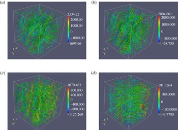
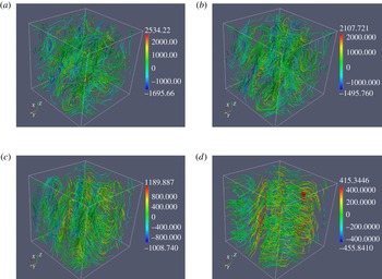
on figure 2. It is also clearly visible on the instantaneous streamlines of the flow at
 $Ha=224$
and
 $Ha=448$
(figures 3 and 4 at
 $t={\it\tau}_{J}$
). Significant variations along the
 $z$
direction exist until approximately
 $t\simeq 1.5{-}2{\it\tau}_{2D}(l)\simeq 5{-}10{\it\tau}_{J}$
for all values of
 $Ha$
. This reflects the prominent contribution of the large scales to the RMS velocity fluctuations, and confirms that large scales indeed become quasi-two-dimensional in this typical time. In the rest of the paper, we shall denote this phase as the three-dimensional phase. After this phase, large columnar structures extending over the entire height of the domain emerge and progressively dominate the dynamics (figures 3 and 4 at
 $t=10{\it\tau}_{J}$
and
 $t=100{\it\tau}_{J}$
). In this phase, which we shall refer to as the two-dimensional phase, both energies and dissipations vary much more slowly than in the three-dimensional phase and the dynamics becomes increasingly dominated by two-dimensional effects.
Instantaneous streamlines of the flow for
 $Ha=224$
at
 $t=0{\it\tau}_{J}$
,
 $1{\it\tau}_{J}$
,
 $10{\it\tau}_{J}$
and
 $100{\it\tau}_{J}$
. The colour scale represents
 ${\it\omega}_{z}$
.

Instantaneous streamlines of the flow for
 $Ha=448$
at
 $t=0{\it\tau}_{J}$
,
 $1{\it\tau}_{J}$
,
 $10{\it\tau}_{J}$
and
 $100{\it\tau}_{J}$
. The colour scale represents
 ${\it\omega}_{z}$
.

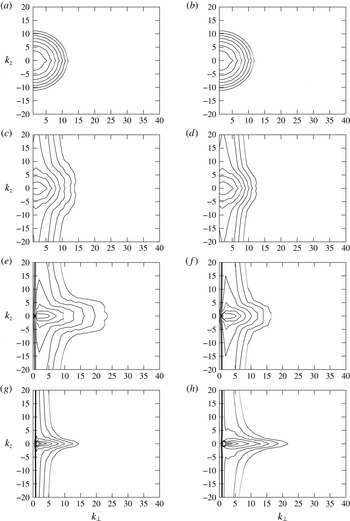
The decay of turbulence towards a state with large quasi-two-dimensional structure is more precisely seen on the evolution of two-dimensional Energy spectra
 $E(k_{\bot },k_{z})$
represented on figure 5. Since the basis of eigenmodes we are using is not orthogonal,
 $E(k_{\bot },k_{z})$
had to be obtained from the three-dimensional Fourier transform of the discrete velocity field at all points from the grid and
 $k_{z}\,\,(\neq {\it\kappa}_{z})$
represents the corresponding integer wavelength in the
 $z$
-direction. The presence of residual energy near the
 $k_{\bot }=0$
axis is the trace of the thin Hartmann layer profile, which is made of Fourier modes with high
 $k_{z}$
(but would only require low values of
 ${\it\kappa}_{z}$
in the space of least dissipative modes). The energy is initially distributed homogeneously in the
 $(k_{\bot },k_{z})$
plane. During the three-dimensional phase, moderate to small three-dimensional scales loose most of their energy whilst only large scale fluctuations along
 $z$
retain theirs. The two-dimensional phase sees a much slower process take place, where energy is more and more centred around the
 $k_{z}=0$
axis and extends to ever smaller scales. In other words, smaller and smaller scales become quasi-two dimensional. The effect is more pronounced at higher
 $Ha$
, as the energy is more sharply concentrated around the
 $k_{z}=0$
axis (i.e. the amplitude of three-dimensional fluctuations is further reduced) and the spectrum of quasi-two dimensional scales extends to higher wavelengths
 $k_{\bot }$
. The resulting contours of energy follow the cardioid shape first experimentally observed by Caperan & Alemany (Reference Caperan and Alemany1985), predicted theoretically by Pothérat & Alboussière (Reference Pothérat and Alboussière2006) and numerically found by Burattini et al. (Reference Burattini, Zikanov and Knaepen2010), Pothérat & Dymkou (Reference Pothérat and Dymkou2010), Favier et al. (Reference Favier, Godeferd, Cambon, Delache and Bos2011).
Evolution of the 2-D power spectrum
 $E(k_{\bot },k_{z})$
(a,c,e,g)
 $Ha=224$
, (b,d,f,h)
 $Ha=448$
. The lowest contour is at
 $10^{-7}$
of power contained in the most energetic mode. The ratio of values between two neighbouring contours is 10: (a,b)
 $t=0{\it\tau}_{j}$
, (c,d)
 $t=1{\it\tau}_{j}$
, (e,f)
 $t=10{\it\tau}_{j}$
, (g,h)
 $t=100{\it\tau}_{j}$
.

5. Three-dimensional phase
In this section, we shall characterise the three-dimensional phase only. For the time being, the analysis shall be restricted to cubic domains of size
 $L$
with Hartmann walls, or with periodic boundary conditions when specified.
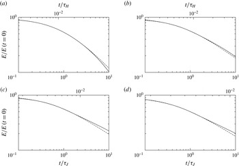
Evolution of total kinetic energy, normalised by its value at
 $t=0$
(solid line). The dashed line represents the fitted law of the form
 $a(1+bt)^{c}$
over interval
 $[0.2,2{\it\tau}_{J}]$
; (a)
 $Ha=112$
; (b)
 $Ha=224$
; (c)
 $Ha=448$
; (d)
 $Ha=896$
.

5.1. Total kinetic energy
Figure 6 presents the evolution of the total kinetic energy in this phase for different values of
 $Ha$
. To compare this evolution to Okamoto et al. (Reference Okamoto, Davidson and Kaneda2010)’s laws for the decay of unbounded, three-dimensional and initially isotropic MHD turbulence, we have fitted the evolution of energy to laws of the form
 $a(1+bt)^{c}$
in ranges from
 $0.05{\it\tau}_{J}$
to up to
 $2{\it\tau}_{J}$
(
 $a$
,
 $b$
and
 $c$
are real constants). All values of
 $c$
are presented in table 2. Okamoto et al. (Reference Okamoto, Davidson and Kaneda2010) showed that in the limit
 $N\rightarrow \infty$
, exponent
 $c$
should be equal to
 $1/2$
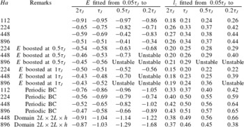
. In our cases, we obtain the best fits for
 $c=0.95$
, 0.75, 0.69 and 0.50 for
 $Ha=112$
, 224, 448 and 896 respectively, over
 $[0.05{\it\tau}_{J},{\it\tau}_{J}]$
. This fit is also relatively robust to a variation of the fitting interval, as exponents decrease only slightly when the interval is extended to
 $[0.05{\it\tau}_{J},2{\it\tau}_{J}]$
. From this, we infer that the decay of turbulence between walls is in line with these authors’ prediction over a duration of about
 ${\it\tau}_{J}$
. Values of
 $c$
are however slightly higher for cases with periodic boundary conditions over this interval, which suggests that the influence of the walls is present but moderate for
 $t\lesssim {\it\tau}_{J}$
. This phase corresponds to roughly 25–50 % of the time interval where we identified strong three-dimensionality in the profiles of RMS velocity fluctuations (figure 2). From times
 $t>{\it\tau}_{J}$
, by contrast, the kinetic energy tends to decay at a slightly slower rate than predicted by Okamoto et al. (Reference Okamoto, Davidson and Kaneda2010) in all cases. This is an indication that some of the turbulent structures interact with the walls, as they become stretched vertically under the effect of diffusion by the Lorentz force. The energy of these structures is dissipated partly by the action of eddy currents recirculating in the Hartmann layers. The Hartmann friction mechanism is typically
 $Ha$
times slower than Joule dissipation, which would be the unique electromagnetic dissipation mechanism if these structures were not in contact with the wall. This explains that the decay of energy slows down for
 $t\gtrsim {\it\tau}_{J}$
.
All cases where the energy was boosted during the three-dimensional phase exhibit a similar behaviour to cases where the energy was left to decay from the start. Nevertheless, for all of them, the value of the
 $c$
coefficient fitted over intervals of
 ${\it\tau}_{J}$
or more is lower than for their counterpart without energy boost. Furthermore, the later the energy is boosted, the lower the value of
 $c$
. This slower decay reflects the influence of the anisotropy of the boundary conditions: at the time of the energy boost, the flow recovers the same energy as at
 $t=0$
but conserves the anisotropy that has developed during the initial decay, before the energy was boosted. Consequently, vortices are more elongated, interaction with the walls is more significant and the slower friction in the Hartmann layers represents a more important fraction of the dissipation. It is for the same reason that cases initialised with a quasi-two-dimensional field show a much slower energy decay, due to the near absence of Joule dissipation in the bulk. In the long term however, energy eventually decays a the same rate as for the other initial conditions.
Fitted values for constant
 $c$
in Okamoto et al. (Reference Okamoto, Davidson and Kaneda2010)’s laws of the form
 $a(bt+1)^{c}$
for the decay of total kinetic energy and the growth of integral scale
 $l_{z}$
. Cases where the formal error of the least squares method was greater than 20 % are marked as ‘unstable’.

(a,c,e,g) Evolution of the kinetic energy in cases with walls (solid lines), periodic boundary conditions (dashed line). (b,d,f,h) Ratio of viscous to Joule dissipation in cases with walls (solid line) and periodic boundary conditions (dashed line), fraction of the dissipation taking place in the Hartmann layers in cases with wall (dotted lines). On all graphs, the shorter curves represent cases with walls where energy was boosted at
 $t=0.5{\it\tau}_{J}$
(short dashed line: Joule to viscous dissipation, short dash-dotted line: fraction of dissipation in the Hartmann layers), at
 $Ha=224,448$
dotted lines (c,e), double dash and dashed dotted lines (d,f) correspond to cases initiated with quasi-two-dimensional turbulence; (a,b)
 $Ha=112$
; (c,d)
 $Ha=224$
; (e,f)
 $Ha=448$
; (g,h)
 $Ha=896$
.

5.2. Dissipation
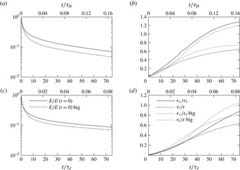
Initially, the kinetic energy is mainly dissipated ohmically and the initial ratio of viscous to Joule dissipation scales as
 ${\sim}1/Ha$
. As the flow becomes more two-dimensional, both viscous and Joule dissipations diminish in the bulk of the flow (between the Hartmann layers). Conversely, dissipation in the Hartmann boundary layers increases as more and more structures interact with the walls. Consequently, the main contribution from the total dissipation ends up coming from the Hartmann layers (see figure 7). For
 $Ha=112$
, 224, 448 and 896 dissipation in the layers becomes larger than in the bulk at
 $t=25{\it\tau}_{J}$
,
 $37.6{\it\tau}_{J}$
,
 $45.1{\it\tau}_{J}$
and
 $54{\it\tau}_{J}$
, respectively. However in the Hartmann layers the Joule dissipation is nearly the same as viscous dissipation. Therefore the global ratio of viscous to Joule dissipation
 ${\it\epsilon}_{{\it\nu}}/{\it\epsilon}_{J}$
increases with time. The value of this ratio becomes larger than unity for
 $t=6.3{\it\tau}_{J}$
,
 $19{\it\tau}_{J}$
,
 $50.1{\it\tau}_{J}$
and
 $88{\it\tau}_{J}$
(or equivalently at
 $t=0.028{\it\tau}_{H}$
,
 $0.042{\it\tau}_{H}$
,
 $0.055{\it\tau}_{H}$
and
 $0.1{\it\tau}_{H}$
) for
 $Ha=112$
,
 $224$
,
 $448$
and
 $896$
, respectively. In all cases, the ratio
 ${\it\epsilon}_{{\it\nu}}/{\it\epsilon}_{J}$
tends to an asymptotic value of
 ${\sim}1.3$
after a time of the order of
 $0.5{\it\tau}_{H}$
. From this perspective, the dissipation behaves as in a three-dimensional flow during a period of time that is longer than the time scale of three-dimensional Joule dissipation
 ${\it\tau}_{J}$
, but shorter than that of two-dimensional effects
 ${\it\tau}_{H}$
. This intermediate time scale is an indication that although large scales become two-dimensional over a time of the order of
 ${\it\tau}_{2D}(l_{0})=2{\rm\pi}{\it\tau}_{J}$
, smaller scales remain three-dimensional during a significantly longer period of time. After
 $t>1.5{-}2{\it\tau}_{2D}$
, the contribution of the large scales to the total dissipation comes mostly from the Hartmann layer, where it is weak, whereas the contribution of the small scales consists of stronger Joule dissipation in the bulk. Joule dissipation therefore remains higher than viscous dissipation until this contribution has significantly reduced, which occurs on a time scale of, at most,
 ${\it\tau}_{H}$
(see § 2.2).
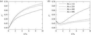
Evolution of integral length scales
 $l_{z}$
(a) and
 $l_{\bot }$
(b) in the presence of Hartmann walls. The evolution of integral length scales at later times, into the quasi-2-D phase is represented on figure 14.

5.3. Integral length scales
Figure 8 (top) shows the initial evolution of the longitudinal integral length scale in the
 $z$
direction
 $l_{z}$
, and in the direction orthogonal to the magnetic field
 $l_{\bot }$
. These are respectively defined as:
 $$\begin{eqnarray}\displaystyle l_{z} & = & \displaystyle \frac{\displaystyle \iint u_{z}(x,y,z)u_{z}(x,y,z+z^{\prime })\,\text{d}V\,\text{d}z^{\prime }}{\displaystyle \int u_{z}^{2}(x,y,z)\,\text{d}V}\end{eqnarray}$$
 $$\begin{eqnarray}\displaystyle l_{\bot } & = & \displaystyle \frac{1}{2}\left(\frac{\displaystyle \iint u_{x}(x,y,z)\cdot u_{x}(x+x^{\prime },y,z)\,\text{d}V\,\text{d}x^{\prime }}{\displaystyle \int u_{x}^{2}(x,y,z)\,\text{d}V}\right.\nonumber\\ \displaystyle & & \displaystyle +\,\left.\frac{\displaystyle \iint u_{y}(x,y,z)\cdot u_{y}(x,y+y^{\prime },z)\,\text{d}V\,\text{d}y^{\prime }}{\displaystyle \int u_{y}^{2}(x,y,z)\,\text{d}V}\right).\end{eqnarray}$$
 $\boldsymbol{u}(x,y,z)$
is non-zero between the walls only (
 $-1/2\leqslant z\leqslant 1/2$
). The initial growth of
 $l_{z}$
can be again fitted with the formula
 $a(1+bt)^{c}$
. Except for
 $t<0.2{\it\tau}_{J}$
, the fitted value of
 $c$
is significantly smaller than Okamoto et al. (Reference Okamoto, Davidson and Kaneda2010)’s theoretical value of 0.5. It is also strongly dependent on the fitting interval for
 $Ha=224$
, 448 and 896. For
 $Ha=112$
, the integral length scale
 $l_{z}$
grows even more slowly with a fitted value down to
 $c\approx 0.18$
over
 $[0.05,2{\it\tau}_{J}]$
. This behaviour indicates a very strong influence of the walls on the growth of
 $l_{z}$
from the outset of the decay. It is somewhat remarkable that, despite this early influence of the walls on
 $l_{z}$
, the energy decay shows little influence of the walls during as long as
 ${\it\tau}_{J}$
–
 $2{\it\tau}_{J}$
. During this initial stage
 $l_{z}$
also grows faster for larger values of
 $Ha$
, with indication that at
 $Ha=224$
, it is already close to its asymptotic behaviour (in the sense of large
 $Ha$
). For
 $t\gtrsim 1.5{\it\tau}_{J}$
, the growth of
 $l_{z}$
slows significantly. As in the case of the energy, this is due to the increasingly wide range of scales reaching the walls during the two-dimensionalisation process, and whose growth in thus impeded in the
 $z$
direction.
With periodic boundary conditions, the fitted value of exponent
 $c$
is higher than with Hartmann walls. It is close to the theoretical value of 0.5 at high
 $Ha$
for
 $t<{\it\tau}_{J}$
, and decreases thereafter. Unlike cases with walls, this behaviour is quite insensitive to the fitting interval for
 $t<{\it\tau}_{J}$
, which confirms the validity to Okamoto et al. (Reference Okamoto, Davidson and Kaneda2010)’s law at high
 $Ha$
over at most one Joule time. The validity of this law also indicates that the parameter
 $l_{\bot }(t=0)/L$
was chosen sufficiently small to observe the main features of three-dimensional unbounded turbulence in a periodic domain. However, the fact that this exponent is higher with periodic boundary conditions than with walls suggests that eddy currents circulating between the Hartmann layer and the bulk (when walls are present) strongly increase the influence of the boundaries from the outset, compared to the periodic case where this effect is absent.
The integral length scale
 $l_{\bot }$
grows very slowly during the decay. This is consistent with the prediction of Okamoto et al. (Reference Okamoto, Davidson and Kaneda2010) of a growth as
 $(t/{\it\tau}_{J})^{3/14}$
. However such a small exponent is difficult to quantify on a time scale of the order of
 ${\it\tau}_{J}$
, where it is expected to be valid. Furthermore,
 $l_{\bot }$
evolves slowly all the way through our calculations, with no clear evidence of a different behaviour when the flow is close to two-dimensional than when it is three-dimensional.
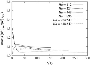
Evolution of the maximum of
 $\langle \boldsymbol{u}_{\bot }^{2}\rangle _{xy}/\langle \boldsymbol{u}_{\bot }^{2}\rangle _{xyz}$
(as represented on figure 2).

6. Quasi-two dimensional phase
We shall now describe the later stage of the flow evolution where it approaches a quasi-two dimensional behaviour, and characterise this asymptotic regime.
6.1. Velocity profiles
When this stage is reached, the spatial RMS over all
 $(x,y)$
of the profile along
 $z$
of
 $\boldsymbol{u}_{\bot }$
have already been considerably smoothed out during the three-dimensional phase of the decay (see figure 2). In every case, we were able to identify a time
 ${\it\tau}_{Q2D}$
, from which the profile starts to flatten monotonically without qualitatively changing shape. This type of decay would be expected from a flow mostly governed by two-dimensional dynamics.
 ${\it\tau}_{Q2D}$
was defined as the time at which the maximum value in the velocity profile starts decreasing monotonically. It was found at
 $19.3{\it\tau}_{J}~(=\,0.17{\it\tau}_{H})$
,
 $18.8{\it\tau}_{J}~(=0.168{\it\tau}_{H})$
,
 $65.2{\it\tau}_{J}~(=0.145{\it\tau}_{H})$
and
 $98{\it\tau}_{J}~(=0.11{\it\tau}_{H})$
for
 $Ha=112$
, 224, 448 and 896, respectively. The fact that it obeys a time scale of approximately
 $0.15{\it\tau}_{H}$
, which is commensurate with the two-dimensional time scale
 ${\it\tau}_{H}$
, indicates that the large scales only acquire a two-dimensional dynamics once a significant part of the spectrum is close to being two-dimensional (since from § 2.2, two-dimensionalisation of the whole spectrum is expected to occur over a period of the order of
 ${\it\tau}_{H}$
). For
 $t>{\it\tau}_{Q2D}$
, the evolution of the shape of the profiles is practically unaffected by those smaller scales that still retain a three-dimensional behaviour at this stage of the decay.
Remarkably, in none of the cases did we find that the profile was quasi-two-dimensional after
 $t\gtrsim 0.5{\it\tau}_{H}$
(although such very long times could not be reached for
 $Ha\geqslant 448$
). Instead, all profiles seem to have reached a barrel-like shape after
 $t\sim 50{\it\tau}_{J}$
, which evolves only very slowly after this time. Also the shape of the profile is flatter for the larger values of
 $Ha$
. This shape was first theorised by Pothérat et al. (Reference Pothérat, Sommeria and Moreau2000) and numerically observed by Mück, Günter & Bühler (Reference Mück, Günter and Bühler2000). This appears equally true whether turbulence is initialised in a three-dimensional of a quasi-two dimensional state. This effect stems from eddy currents recirculating between the Hartmann layers and the core. These currents are driven along the axis of columnar vortices. Their leak into the core drives differential rotation between horizontal planes of the vortex leading to the barrel-shaped profile (see also Pothérat Reference Pothérat2012). Since the effect is driven by currents recirculating between the bulk and the Hartmann layer scaling as
 $Ha^{-1}$
, it is less marked at high
 $Ha$
.
The intensity of the barrel effect can be measured through the relative value of the maximum in the profile. The evolution of this quantity is shown on figure 9. First, this graph confirms quantitatively that the barrel effect is less pronounced at higher
 $Ha$
. Second, the graph also confirms the invariance of the barrel shape of the large scales beyond
 $t\sim 50{\it\tau}_{J}$
. This appears to be verified over at least
 $200{\it\tau}_{J}$
, even though the total energy drops by a factor of up to a couple of orders of magnitude during this interval, depending on the value of
 $Ha$
. This remarkable feature shows that even at high
 $Ha$
, a form of three-dimensionality subsists a large times, even in the large scales, and no matter the initial amount of three-dimensionality in the flow.
Finally, we verified that cases where the energy was boosted at
 $t=0.5{\it\tau}_{J}$
,
 $t={\it\tau}_{J}$
and those where the flow was initialised in a quasi-two dimensional state exhibit the same behaviour, which confirms robustness to initial conditions of this scenario.
6.2. Energy
In all calculated cases (with and without energy boost, quasi-two- or three-dimensional initial conditions), the evolution of the total kinetic energy in the late phase can be described as an exponential decay with slowly changing time scale. However, even at the latest time in our calculations, this time scale does not seem to converge towards a clear asymptotic value. This indicates that even for
 $t\gtrsim 0.5{\it\tau}_{H}$
, when all structures could theoretically be expected to have been diffused across the channel height, the decay is still not entirely dominated by dissipation in the Hartmann layers. The origin of the extra dissipation shall be determined by examining different types of dissipation in § 6.3.
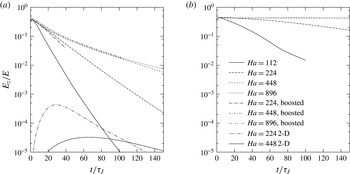
Evolution of
 $E_{z}/E$
for cases with walls (a) and with periodic boundaries (b).

The energy associated to the
 $z$
component of the velocity is represented on figure 10. For all cases with Hartmann walls,
 $E_{z}/E$
tends rapidly to zero, which is consistent with the experimental findings of Kolesnikov & Tsinober (Reference Kolesnikov and Tsinober1974) for turbulence in a duct. By contrast, for experiments where turbulence was kept far from Hartmann walls (Alemany et al.
Reference Alemany, Moreau, Sulem and Frish1979) and for simulations with periodic boundary conditions rather than walls, (Schumann Reference Schumann1976; Burattini et al.
Reference Burattini, Zikanov and Knaepen2010) show a transfer of energy to the velocity component along
 $\boldsymbol{B}$
, which results in a maximum in
 $E_{z}/E$
, followed by a much slower decay than in the case with walls. This supports the explanation put forward by Burattini et al. (Reference Burattini, Zikanov and Knaepen2010) who hypothesised that the difference between these two scenarios was due to the presence of the Hartmann walls. The question of how much transport along
 $\boldsymbol{B}$
remains asymptotically can be further analysed through the evolution of the skewness coefficient
 $$\begin{eqnarray}S=\frac{1}{35}\left(\frac{15}{\hat{{\it\epsilon}}}\right)^{3/2}\hat{{\it\Gamma}},\end{eqnarray}$$
where
 $$\begin{eqnarray}\displaystyle & \displaystyle \hat{{\it\Gamma}}=\mathop{\sum }_{\boldsymbol{k}}2k^{2}\hat{\boldsymbol{q}}(\boldsymbol{k})\boldsymbol{\cdot }\hat{\boldsymbol{u}}^{\ast }(\boldsymbol{k}), & \displaystyle\end{eqnarray}$$
 $$\begin{eqnarray}\displaystyle & \displaystyle \hat{{\it\epsilon}}=\mathop{\sum }_{\boldsymbol{k}}2k^{2}\hat{\boldsymbol{u}}(\boldsymbol{k})\boldsymbol{\cdot }\hat{\boldsymbol{u}}^{\ast }(\boldsymbol{k}), & \displaystyle\end{eqnarray}$$
 $\boldsymbol{q}(\boldsymbol{k})$
is the Fourier transform of nonlinear term
 $(\boldsymbol{u}\boldsymbol{\cdot }\boldsymbol{{\rm\nabla}})\boldsymbol{u}$
. Schumann (Reference Schumann1976) found
 $S$
to remain constant at large times. This author interpreted this behaviour as an evidence that transport of
 $E_{z}$
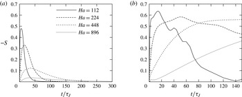
became important at large times. Our computed evolution of
 $S$
is shown on figure 11. In the domain with periodic boundary conditions, we recover Schumann (Reference Schumann1976)’s findings at high
 $Ha$
that
 $S$
seems to converge to a constant asymptotic value. However, as in this authors’ work, we were not able to compute
 $S$
for
 $t>0.5{\it\tau}_{H}$
at the highest value of
 $Ha$
, so the two-dimensionalisation process may not be entirely complete at the end of this particular calculation. The decay of
 $-S$
observed in the later stages of the decay for
 $Ha\leqslant 224$
suggests that
 $S$
may in fact evolve on a time scale significantly longer than the duration of our calculations, and eventually tend to zero. Simulations with Hartmann walls, by contrast, exhibit a fast decay of
 $S$
and it is readily visible that
 $S\rightarrow 0$
in all calculated cases. Together with the fast decay of
 $E_{z}/E$
, this behaviour confirms that the presence of walls results in a very strong suppression of transport along
 $\boldsymbol{B}$
, in contrast to the phenomenology of flows with periodic boundary conditions.
Evolution of skewness
 $S$
for cases with walls (a) and with periodic boundaries (b).

Note that in the two-dimensional phase, both
 $E$
(see figure 7) and
 $E_{z}/E$
appear to decay faster at lower values of
 $Ha$
in the case with walls. It should however be pointed out that in this phase, turbulence decays over a time scale of
 ${\it\tau}_{H}=Ha{\it\tau}_{J}$
, which appears slower at higher
 $Ha$
in units of time normalised by
 ${\it\tau}_{J}$
when it is in fact faster in dimensional time units.
Finaly, in simulations where the total energy in the flow was artificially boosted at
 $t=0.5{\it\tau}_{J}$
(and, we verified,
 $t={\it\tau}_{J}$
) both
 $E$
and
 $E_{z}/E$
exhibit a similar behaviour to the case without energy boost, which confirms the robustness of this phenomenology to initial conditions. Interestingly, when the flow is initialised in a quasi-two-dimensional state (i.e.,
 $E_{z}(0)=0$
), a very weak third component still develops over a time scale significantly longer than that of the three-dimensional phase, before entering the same steep rate of decay as with other initial conditions.
6.3. Dissipation
Asymptotically, the ratio of viscous to ohmic dissipations
 ${\it\epsilon}_{{\it\nu}}/{\it\epsilon}_{J}$
tends to a value of approximately 1.3 for all values of
 $Ha$
(see figure 7). For all cases except
 $Ha=896$
, we observe a maximum in the temporal evolution of this ratio at times
 $0.175{\it\tau}_{H},0.19{\it\tau}_{H},0.25{\it\tau}_{H}$
for
 $Ha=112$
, 224 and 448, respectively. The maximum becomes less pronounced with increasing
 $Ha$
, with the ratio of maximal value of
 ${\it\epsilon}_{{\it\nu}}/{\it\epsilon}_{J}$
to its asymptotic value decreasing from 1.28 at
 $Ha=112$
to 1.04 at
 $Ha=448$
. For
 $Ha=896$
, this maximum is still present for
 $t\sim 0.278{\it\tau}_{H}$
, although even less prominent. This behaviour is very different from that observed in simulations with periodic boundary conditions, where
 ${\it\epsilon}_{{\it\nu}}/{\it\epsilon}_{J}$
increases indefinitely. In both cases the sharp initial increase of this ratio is due to the two-dimensionalisation of smaller and smaller structures. Indeed, from the right-hand side of (2.6), the ratio of dissipations for a structure of wavenumber
 $(k_{\bot },{\it\kappa}_{z})$
is
 ${\it\epsilon}_{{\it\nu}}(k_{\bot },{\it\kappa}_{z})/{\it\epsilon}_{J}(k_{\bot },{\it\kappa}_{z})=Ha^{-2}(1+(k_{\bot }/{\it\kappa}_{z})^{2})$
. While initially
 $k_{\bot }/{\it\kappa}_{z}\sim 1$
,
 $k_{\bot }/{\it\kappa}_{z}$
becomes very large for nearly two-dimensional structures. As time progresses, this becomes true for increasingly larger values of
 $k_{\bot }$
, and so the ratio of total viscous to Joule dissipations
 ${\it\epsilon}_{{\it\nu}}/{\it\epsilon}_{J}$
increases. With periodic boundary conditions, strictly two-dimensional structures (
 ${\it\kappa}_{z}=0$
) can exist and so this ratio is unbounded. In the presence of Hartmann walls, on the other hand, quasi-two-dimensional structures generate little dissipation in the bulk. Most of their dissipation comes from the Hartmann layers, where viscous and Joule dissipation are locally of the same order. This explains that the ratio
 ${\it\epsilon}_{{\it\nu}}/{\it\epsilon}_{J}$
converges to a value of the order of unity.
The presence of the maximum in the evolution of
 ${\it\epsilon}_{{\it\nu}}/{\it\epsilon}_{J}$
at lower values of
 $Ha$
may be attributed to structures that are too small for magnetic diffusion to stretch them up to the walls, i.e., for which at
 $t=0$
,
 $l_{z}^{N}(k_{\bot })=k_{\bot }^{-1}N(k_{\bot })^{1/2}<L$
(Pothérat & Klein Reference Pothérat and Klein2014). These initially generate a large contribution to the ratio
 ${\it\epsilon}_{{\it\nu}}/{\it\epsilon}_{J}$
over a time scale of the order of
 ${\it\tau}_{2D}(k_{\bot })$
, which is longer than the two-dimensionalisation time of the large scales
 ${\it\tau}_{2D}(l_{0})$
but shorter than the decay time of quasi-two-dimensional structures
 ${\it\tau}_{H}$
. For
 $t\sim 0.5{\it\tau}_{H}$
, these structures have lost most of their energy and the surviving structures extend across the whole channel. As
 $Ha$
increases, structures that remain three-dimensional during their entire life span are confined to a region of the spectrum of higher and higher length scale and their contribution to the total dissipation progressively vanishes. This explains that the maximum is less pronounced at higher values of
 $Ha$
, and also that it occurs at later times.
More details on the asymptotic state can be obtained by inspecting the ratio of the total dissipation coming from the Hartmann layers to that coming from the bulk (figure 7). Asymptotically, the dissipation comes dominantly from Hartmann layers because the flow becomes close to quasi-two dimensional at all values of
 $Ha$
investigated here. However, approximately 20 % of the dissipation still takes place in the bulk asymptotically. It is tempting to check whether the residual three-dimensionality due to the barrel effect noted on the velocity profiles (§ 6.1) is responsible for this extra dissipation: since it is driven by currents in the Hartmann layers that recirculate in the bulk, Joule dissipation must be associated to it. Current conservation implies that the current densities in the bulk
 $J^{C}$
and the Hartmann layers
 $J^{H}$
must satisfy
 $J^{H}/J^{C}\sim Ha$
and so the contributions to Joule dissipation from the core and the Hartmann layers must be in a ratio of
 ${\it\epsilon}_{J}^{H}/{\it\epsilon}_{J}^{C}\sim Ha$
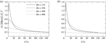
. This scaling is insufficient to explain the relatively high level of dissipation observed in the bulk: this discards the barrel effect as the residual source of dissipation. To find out the origin of this extra dissipation, we calculated non-dimensional quantity
 $2Ha^{-1}(L/l_{\bot }^{{\it\nu}})^{2}$
, which, from (2.15), represents the actual ratio of quasi-two-dimensional viscous friction to Hartmann friction. It transpires that this ratio converges towards a constant value around 0.2, regardless of the case considered (see figure 13). This implies that extra dissipation in the bulk results from viscous friction incurred by gradients of the
 $x$
and
 $y$
components of the velocity in the
 $x$
and
 $y$
directions. This extra dissipation also explains that the energy does not decay exponentially even for
 $t\gtrsim 0.5{\it\tau}_{H}$
, as would be expected if Hartmann friction was the exclusive dissipation mechanism. Interestingly, the ratio
 $2Ha^{-1}(L/l_{\bot }^{{\it\nu}})^{2}$
behaves in roughly the same way whether Hartmann walls are present or not. Even though Hartmann friction is absent when boundary conditions are periodic in all three spatial directions, it still gives a normalised measure of the level of two-dimensional viscous dissipation, which appears to be the same with and without Hartmann walls. Furthermore, our simulations show that in the Hartmann layers, Joule and viscous dissipations are asymptotically the same up to few percent. Therefore viscous dissipation due to horizontal velocity gradients also explains that the ratio
 ${\it\epsilon}_{{\it\nu}}/{\it\epsilon}_{J}$
remains greater than unity even for
 $t\gtrsim 0.5{\it\tau}_{H}$
, when two-dimensionalisation is expected be complete over the whole spectrum of length scales.
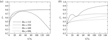
6.4. Integral length scales
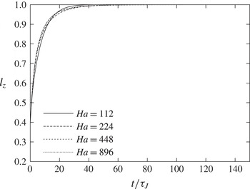
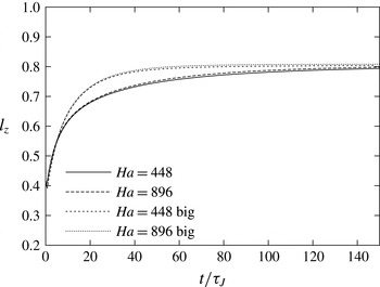
Figures 14 and 15 shows the evolution of
 $l_{z}$
up to the later stages where
 $t>{\it\tau}_{H}$
. For large values of
 $Ha$
,
 $l_{z}$
tends asymptotically to a value of approximately 0.8. By contrast, in simulations with periodic boundary conditions
 $l_{z}$
asymptotically tends to 1. At high
 $Ha$
the Hartmann layers are laminar and not affected by inertia present in the core. The classical theory for these layers then implies that the velocity normal to the wall in the layer is
 $\mathit{O}(Ha^{-1})$
and this imposes a region of very low values of
 $u_{z}$
near the walls. By contrast, residual velocity may exist in the core and so the
 $z$
-component of the velocity cannot be correlated over the entire width of the channel (see profiles of vertical velocity on figure 2). This effect is absent with periodic boundary conditions, where a constant through-flow can exist in the
 $z$
-direction, which allows values of
 $l_{z}$
close to 1.
The convergence of
 $l_{z}$
for cases bounded by walls becomes less smooth for lower values of
 $Ha$
. For
 $Ha=112$
,
 $l_{z}$
shows no signs of convergence to a finite value. It starts decreasing around
 $t\sim 45{\it\tau}_{J}$
and still decreases at
 $t\simeq 1.5{\it\tau}_{H}$
. This behaviour is caused by Ekman pumping in large quasi-two dimensional vortices. This effect tends to produce vertical profiles of
 $u_{z}$
that are antisymmetric with respect to the mid-plane. According to (5.2), Ekman pumping reduces the value of
 $l_{z}$
as its definition is based on
 $u_{z}(z)$
(see figure 2). The intensity of Ekman pumping is driven by inertia but damped by the Lorentz force: Pothérat et al. (Reference Pothérat, Sommeria and Moreau2000) showed that it scaled as
 $u_{z}/u_{\bot }\sim Ha^{-2}N^{-1}$
. This explains that this effect is only noticeable at the lowest value of
 $Ha$
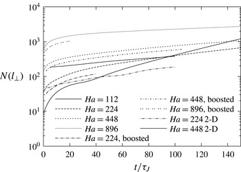
. This also suggests that ultimately, since the interaction parameter
 $N(t)$
diverges asymptotically (see figure 12), Ekman pumping should progressively disappear and
 $l_{z}$
may increase again. The evolution of
 $l_{z}$
on figure figure 14 however implies that this may only take place after a very long time, beyond the reach of our calculations. Also, since
 $E_{z}/E$
is very small in the later stages of the decay,
 $l_{z}$
relies in fact on low values of
 $u_{z}$
and only reflects a weak component of the flow, from the energy point of view. Despite its relative weakness, Ekman pumping is responsible for the larger values of
 $l_{\bot }$
at
 $Ha=224$
and more noticeably at
 $Ha=112$
(figure 14). Ekman pumping indeed transports momentum radially outward of large structure thus increasing their effective size in the horizontal plane (Sommeria Reference Sommeria1988).
Evolution of interaction parameter
 $N={\it\sigma}B^{2}l_{\bot }/({\it\rho}U(t))$
, where
 $U(t)=(\int _{(x,y,z)\in [0,L]^{3}}\boldsymbol{u}^{2}\,\text{d}V)^{1/2}.$

Ratio of effective dissipation by 2-D viscous friction to Hartmann friction: case with Hartmann wall (a) and case with periodic boundary conditions (b). With periodic conditions, this quantity represents the normalised 2-D dissipation only, as Hartmann friction is absent.

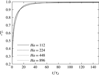
From this phenomenology,
 $l_{z}$
appears dominated by the dynamics of secondary flows but does not reflect accurately the dimensionality of turbulence. We argue that this calls for a more suitable quantity to characterise the growth of vertical scales along the
 $z$
direction. We propose that such a quantity may be defined as:
 $$\begin{eqnarray}l_{z}^{\bot }=\frac{\displaystyle \iint \boldsymbol{u}_{\bot }(x,y,z)\boldsymbol{u}_{\bot }(x,y,z+z^{\prime })\,\text{d}V\,\text{d}z^{\prime }}{\displaystyle \int u_{\bot }^{2}(x,y,z)\,\text{d}V}.\end{eqnarray}$$
As in (5.2),
 $l_{z}^{\bot }$
is evaluated in cases with walls by assuming a non-zero velocity
 $\boldsymbol{u}(x,y,z)$
between the walls only (
 $-1/2\leqslant z\leqslant 1/2$
). The temporal evolution of
 $l_{z}^{\bot }$
is shown on figure 16 for decaying turbulence between walls. In contrast to
 $l_{z}$
, it asymptotically converges to 1 for all values of
 $Ha$
, and curves remain very close to each other in all stages of the evolution. During the initial stage,
 $l_{z}^{\bot }$
grows over a time scale of
 ${\it\tau}_{2D}(l)$
, which does reflect the two-dimensionalisation of the large scales.
 $l_{z}^{\bot }$
reaches a value of 0.9 at
 ${\sim}15{\it\tau}_{J}$
for all values of
 $Ha$
, and its subsequent evolution in the quasi-two-dimensional phase is only slow. This indicates that
 $l_{z}^{\bot }$
is only weakly affected by the two-dimensionalisation of smaller scales, unlike the total kinetic energy and the dissipation.
7. Robustness analysis
In order to focus on the long-term evolution of the decay of turbulence whilst keeping computational costs reasonable, we have conducted our study with a domain of limited size and used only a single set of isotropic initial conditions per type of computation. Ongoing experiments on decaying turbulence conducted on the FLOWCUBE setup (Pothérat & Klein Reference Pothérat and Klein2014) show that reliable quantitative laws require ensemble averaging on a large number of initial conditions, which cannot be done numerically. Nevertheless, we shall now estimate the impact of the domain size in the
 $x{-}y$
directions, and of the particular set of initial conditions used on the mechanisms found, by examining the result of two simulations in a channel four times bigger (dimensions
 $2L\times 2L\times L$
), with different random initial conditions (albeit with the same statistical properties as in the cases where energy has not been boosted), and slightly smaller initial Reynolds number (see table 1).
Evolution of integral length scales
 $l_{z}$
(a) and
 $l_{\bot }$
(b) for the simulations with walls.

Evolution of integral length scale
 $l_{z}$
for periodic cases.

Evolution of integral length scale
 $l_{z}^{\bot }$
for simulations with walls.

Evolution of energy (a,c) and dissipation rates (b,d) in smaller and larger domains (marked ‘big’ in the legend), with Hartmann walls: (a,b)
 $Ha=224$
; (c,d)
 $Ha=448$
.

Evolution of
 $l_{z}$
in smaller and larger domains (marked ‘big’ in the legend) with Hartmann walls.

Comparison between energy decay and dissipation ratios in small and large domains is shown on figure 17. The decay follows a similar profile in both cases. In the three-dimensional phase, fits to Okamoto et al. (Reference Okamoto, Davidson and Kaneda2010)’s decay laws yields exponents that are consistently higher in the case of a larger domain. Nevertheless, their variations with
 $Ha$
and with the fitting interval are consistent between cases (see table 2). We also noted that actual values of the exponent are sensitive to the lower bound of the fitting interval, but that again, variations with
 $Ha$
and with the fitting interval are consistent between cases, for the same lower bound. This sensitivity can most likely be attributed to the lack of an ensemble average which, as in experiments, would be required for a precise estimate of exponents in Okamoto et al. (Reference Okamoto, Davidson and Kaneda2010)’s decay laws.
Nevertheless, the interval of validity of the these laws can still be estimated by varying the upper bound of the fitting interval, and this yields consistent results between cases and choices of fitting interval. Most importantly, the main properties of the decay outlined throughout the paper appear consistent between the two sets of simulations: the duration of the three-dimensional phase is of the order of
 ${\it\tau}_{2D}(l_{0})$
in both cases, and the asymptotic behaviours are identical as decays of energy are parallel to each other. Similarly, Ratios of dissipations (dissipation in the Hartmann layer to dissipation in the bulk and viscous to Joule dissipation), depict the same phenomenology as the evolution of energy: time scales are identical for both domains and evolution curves are parallel. The integral length scale (figure 18) also evolves initially in a similar fashion in both cases and converges to the same asymptotic value. In conclusion to this short analysis, although it is difficult to precisely verify the numerical value of the exponents predicted in Okamoto et al. (Reference Okamoto, Davidson and Kaneda2010)’s laws, the scenario for the decay outlined through the analysis of the cubic domain seems robust to changes in numerical parameters.
8. Conclusion
Using a new type of spectral method based on the least dissipative eigenmodes of the dissipation operator, we were able to perform direct numerical simulations of freely decaying turbulence in a strong magnetic field, between two Hartmann walls. The decay exhibits three- and a two-dimensional phases with an overlap: the former is dominated by the two-dimensionalisation process, where diffusion by the Lorentz force stretches vortices until they reach the Hartmann walls. This process is highly dissipative and leads to a rapid variation of energy and of the integral length scale along
 $\boldsymbol{B}$
. Larger scales are two-dimensionalised more quickly than smaller ones. Once the large scales of turbulence are close to two-dimensional (after
 ${\it\tau}_{2D}(l_{0})$
) the flow starts exhibiting a two-dimensional dynamics, where dissipation mostly takes place in the Hartmann boundary layers, with a slower characteristic time scale
 ${\it\tau}_{H}=Ha{\it\tau}_{J}$
. However since it can take up to
 ${\it\tau}_{H}$
for small scales to adopt a two-dimensional dynamics, there is no clear separation between these two phases and both two- and three-dimensional dissipation mechanisms coexist long after
 ${\it\tau}_{2D}(l_{0})$
. We were able to single out several important features of this phenomenology: first, the presence of the walls turned out to impede the growth of
 $l_{z}$
right from the earliest stages of the decay, whereas the decay of energy remained roughly in line with Okamoto et al. (Reference Okamoto, Davidson and Kaneda2010)’s law of
 $E\sim t^{-1/2}$
for unbounded turbulence in the limit of high
 $Ha$
, during around one Joule time.
Second, the energy associated to the velocity component across the channel is very strongly suppressed:
 $E_{z}/E$
tends to 0 much faster than for unbounded turbulence. This result is consistent with Kolesnikov & Tsinober (Reference Kolesnikov and Tsinober1974)’s experiments and confirms Burattini et al. (Reference Burattini, Zikanov and Knaepen2010)’s hypothesis that the presence of walls is responsible for the suppression of the third component. Further evidence of this suppression is visible in the long term behaviour of the skewness which tends to 0 in the case with walls. With periodic boundary conditions, by contrast, the skewness remains high and almost constant during the entire two-dimensionalisation phase, of order
 ${\it\tau}_{H}$
. For
 $Ha\leqslant 224$
, it subsequently decays, possibly to zero. Previous studies did not extend past this phase and concluded that the skewness remained constant in the later stages of the decay. This may apparently not be the case from the point where boundaries (even periodic) exert any noticeable influence on the flow. Nevertheless, since the time scale of this decay
 ${\it\tau}_{H}$
, is much longer than our calculations at high
 $Ha$
, and than calculations in previous studies, it remains unclear whether the skewness indeed remains constant past the two-dimensional phase with periodic boundaries for
 $Ha>224$
.
Thirdly, long into the ‘two-dimensional phase’, we found that even at the highest value of
 $Ha$
, a form of three-dimensionality subsisted, due to currents recirculating between the Hartmann layers and the bulk. This effect is characterised by the barrel shape visible on the larger structures, as predicted by Pothérat et al. (Reference Pothérat, Sommeria and Moreau2000). Though less pronounced at higher values of
 $Ha$
, our simulations show no evidence of it vanishing at larger times.
Fourthly, in quasi-two dimensional flows dominated by dissipation in the Hartmann boundary layers, the total kinetic energy would be expected to decay exponentially with a time scale of
 ${\it\tau}_{H}$
. However, a true exponential decay of this sort was never observed, even for
 $t\gtrsim {\it\tau}_{H}$
. Remarkably, this discrepancy to a pure exponential decay did not result from the residual three-dimensionality due to the barrel effect, but mostly from viscous friction in the horizontal plane.
At more moderate values of
 $Ha$
(
 $Ha=112$
), secondary flows in large structures significantly affect the decay by increasing the integral length scale in the directions along the channel (perpendicular to
 $\boldsymbol{B}$
). Since, however this effect is driven by two-dimensional inertia, it is expected to vanish at larger times, but was still present after
 $1.5{\it\tau}_{H}$
. When present, it is shown to dominate the behaviour of the integral length scale in the direction of the magnetic field. This prompted us to put forward an alternative definition for this integral length scale that gives a better measure of the flow dimensionality.
Finally, in the main simulations considered here, the flow was initially isotropic and the magnetic field ‘switched on’ at the initial time of the decay. While this approach can be theoretically justified (Moffatt Reference Moffatt1967), it cannot be realised in experiments. In practice, turbulent decay would start from a state of statically steady forced turbulence. The main difference to be expected is the absence of, or a much shorter, three-dimensional phase, since the flow would then already be strongly anisotropic. Our simulations where energy was artificially increased part-way through the three-dimensional phase, and simulations where the flow was initialised in a quasi-two-dimensional state however provide good evidence that the dissipative properties of the later two-dimensional phase are very robust to initial conditions and therefore would probably be similar to those outlined in this paper, if the decay has started from a state of statistically steady MHD turbulence. The footprint of the initial conditions indeed does not survive the three-dimensional phase, other than through slightly different levels of total kinetic energy reached in the long term. The reason is that while the energy results from the cumulated history of dissipative events throughout the decay, the total dissipation, by contrast, only reflects dissipation mechanisms at play at the instant considered.
Acknowledgements
The authors are grateful to the Leverhulme Trust, who supported this work through Research Project Grant ref. F00/732J, to Professor M. K. Verma, who made his Fourier-based spectral code available to them as a basis for the implementation of their novel spectral method, and to Dr B. Teaca both for making the TURBO code available to us and for numerous fruitful coffee-time discussions around its application to this study. A.P. aknowledges support from the Royal Society through the Wolfson Research Merit Award Scheme.