1 Introduction
In various environmental and industrial contexts, the removal of material beneath the surface of a granular substrate can cause the surface above the withdrawal zone to subside and steepen. Examples include mining-induced ground subsidence (Vivanco & Melo Reference Vivanco and Melo2013), and material drainage from granular hoppers or pebble bed reactors (Cleary & Sawley Reference Cleary and Sawley2002; Rycroft et al. Reference Rycroft, Grest, Landry and Bazant2006). If steepening causes the surface inclination to exceed the angle of repose, avalanching will occur. One common example occurs in the upper chamber of an hour glass, where a funnel-shaped avalanching surface forms due to drainage through the underlying narrow throat. In the present work, we examine these phenomena in a simplified geometry: rectangular silos holding grains between two closely spaced smooth walls, making the flows quasi-two-dimensional. Such flows have earlier been investigated using laboratory experiments (Gray & Hutter Reference Gray and Hutter1997; Samadani, Mahadevan & Kudrolli Reference Samadani, Mahadevan and Kudrolli2002; Benyamine et al. Reference Benyamine, Djermane, Dalloz-Dubrujeaud and Aussillous2014; Maiti, Das & Das Reference Maiti, Das and Das2016), continuum models (Staron, Lagrée & Popinet Reference Staron, Lagrée and Popinet2014; Dunatunga & Kamrin Reference Dunatunga and Kamrin2015; Daviet & Bertails-Descoubes Reference Daviet and Bertails-Descoubes2016) and discrete element simulations (Cleary & Sawley Reference Cleary and Sawley2002; Staron et al. Reference Staron, Lagrée and Popinet2014; Zhou, Ruyer & Aussillous Reference Zhou, Ruyer and Aussillous2015).
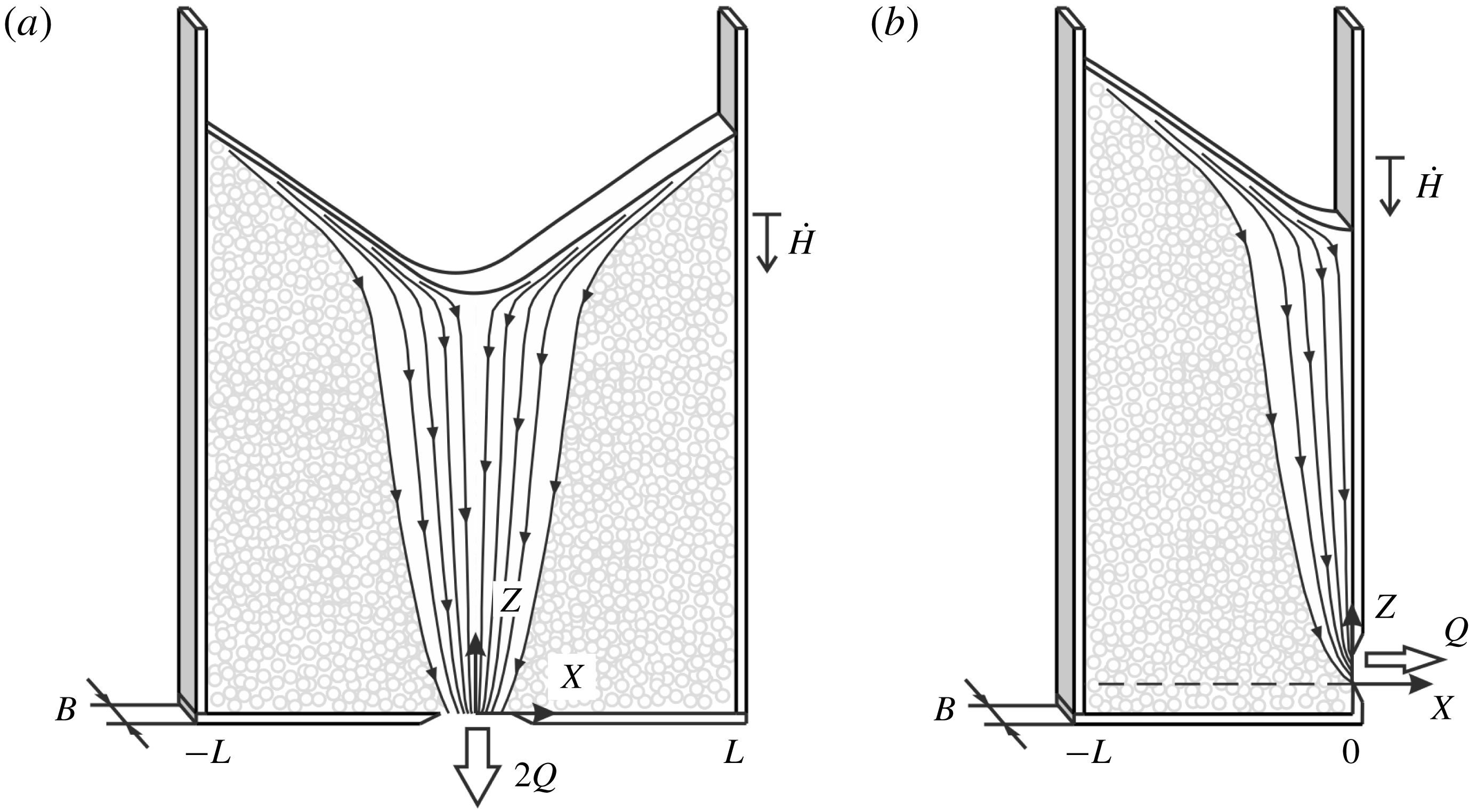
To simplify the problem further, we consider silos of small width to depth ratios, restricting the span of the avalanching layer (figure 1). Experimental observations then suggest that the following simplifications can be made. When drainage at depth through a bottom or side orifice occurs at a constant rate, first, the resulting granular surface flow can be considered quasi-steady. After a starting transient, during which the granular free surface deforms from its initial shape to its avalanching shape, the surface flow becomes nearly steady in a frame of reference descending at constant speed with the free surface. Avalanching thus takes the form of a travelling wave. Because it is driven by a deep subsidence flow that varies spatially with height, the avalanching flow is not perfectly steady. Except for low submergence above the orifice, however, the spatial evolution of this deep flow is gradual, hence the descending avalanching flow experiences forcing changes that are slow with respect to its adaptation time. At any given time over most of its descent history, therefore, the avalanching flow can be approximated as a steadily flowing layer that continually exchanges grains with the substrate through entrainment and detrainment. This makes avalanching flows in narrow silos analogous to other steady granular layer flows subject to erosion and deposition, like flows in rotating drums (Gray Reference Gray2001; Hung, Stark & Capart Reference Hung, Stark and Capart2016) and bounded heaps (Khakhar et al. Reference Khakhar, Orpe, Andresén and Ottino2001; Fan et al. Reference Fan, Umbanhowar, Ottino and Lueptow2013).
In the present paper, we investigate quasi-steady, quasi-two-dimensional silo avalanching flows using a combination of theory and experiment. Using either continuum or discrete models, one could attempt to model together both the deep flow and surface avalanching regions of the phenomenon (see e.g. Staron et al. Reference Staron, Lagrée and Popinet2014). This is however made difficult by the highly different scales that govern the two regions. Whereas the deep flow is steady, slow, and gradually varying in space, the avalanching flow is confined to a thin surface layer featuring faster velocities and steeper velocity gradients. Analogous to the boundary layer approach for viscous and turbulent flows, therefore, we adopt a modelling strategy that couples different equations for different zones of the flow. For the deep flow, we adopt the kinematic model proposed by Nedderman & Tüzün (Reference Nedderman and Tüzün1979), which reduces the problem to the solution of a diffusion equation.
Sketch of the assumed silo configurations: (a) symmetric silo with a centred bottom orifice; (b) asymmetric silo with a side orifice.
To describe surface avalanching, on the other hand, we adopt the model proposed by Capart, Hung & Stark (Reference Capart, Hung and Stark2015) and recently applied by Hung et al. (Reference Hung, Stark and Capart2016) to granular flows in rotating drums. Instead of solving local partial differential equations (Jop, Forterre & Pouliquen Reference Jop, Forterre and Pouliquen2007; Lusso et al.
Reference Lusso, Bouchut, Ern and Mangeney2017; Fernández-Nieto et al.
Reference Fernández-Nieto, Garres-Díaz, Mangeney and Narbona-Reina2018), the model uses depth-integrated equations for the balance of mass, momentum and kinetic energy of the shallow avalanching layer. This model applies to dry, dense, two-dimensional granular flows in narrow channels, over deep erodible deposits, when the flow and bed are composed of the same mono-disperse grains. The model further assumes that the flow is subject to friction along the walls and governed by a linearized form of the viscoplastic
 $\unicode[STIX]{x1D707}(I)$
rheology (da Cruz et al.
Reference da Cruz, Emam, Prochnow, Roux and Chevoir2005; Jop, Forterre & Pouliquen Reference Jop, Forterre and Pouliquen2005), such that the base of the flow coincides with the yield locus. As a result, it cannot describe flows over non-erodible beds (Parez, Aharonov & Toussaint Reference Parez, Aharonov and Toussaint2016; Sarno et al.
Reference Sarno, Carleo, Papa and Villani2018) or the transitions between flow and rest observed for shallow granular layers in wide channels (Pouliquen & Forterre Reference Pouliquen and Forterre2002; Edwards & Gray Reference Edwards and Gray2015).
For the experiments, we adopt a configuration aimed at maximizing the resolution at which the deep and surface flows can be recorded by a high-speed camera. A half-silo geometry is adopted, and the silo is mounted on a motorized traverse to make it rise steadily relative to the camera, keeping the avalanching flow stationary relative to the observation window. Particle tracking velocimetry is then applied to the footage. Averaging of the deep flow and avalanching layer velocity fields is performed in the separate frames of reference in which they can be considered steady.
The paper is structured as follows. In § 2, we describe the theories adopted to model deep flow and surface avalanching, and how they are coupled together. In § 3, we present the experimental set-up, conditions and imaging analysis. In § 4, we compare and discuss results, before drawing conclusions in § 5.
2 Theory
The geometrical conditions considered in the present work are defined in figure 1. We assume silos of rectangular shape, with smooth front and back walls separated by a small gap thickness
 $B$
equal to some multiple (of the order of 10) of the grain diameter
 $D$
. We therefore consider three-dimensional grain configurations, not monolayers. Because the gap is narrow and the walls smooth, however, we can assume that the flow field will be effectively two-dimensional. For simplicity, we consider either the symmetric geometry of figure 1(a), of spanwise width
 $2L$
on either side of a centred bottom orifice, or the asymmetric geometry of figure 1(b) having width
 $L$
and a side orifice at
 $X=0$
. For the near field around the orifice, differences between bottom and side outlets are expected, leading to different variants of the Beverloo relation expressing the rate of outflow in terms of grain diameter, gap thickness and orifice opening (Zhou et al.
Reference Zhou, Lagrée, Popinet, Ruyer and Aussillous2017). Regardless of the case, however, a constant flow rate is obtained when the orifice opening is large enough to prevent jamming, and when the silo free surface is sufficiently high above the orifice. Both conditions will be assumed, hence we consider the outflow rate known and constant. Throughout the silo, only a single type of grains is considered.
Upon starting the silo discharge, grains will descend and converge towards the orifice, drawing down the free surface. Avalanching will then occur once uneven subsidence has steepened the granular free surface beyond its angle of repose. After this initial transient, we consider separately the shallow avalanching layer and the deep flow region comprised between this layer and the orifice near field. Since the outflow rate is constant, flow in the deep region will be assumed steady in the silo frame of reference defined by axes
 $(X,Z)$
. For sufficiently small silo widths
 $L$
, the span of the avalanching flow will be bounded by the side walls. We therefore expect the avalanching layer to attain and maintain a quasi-steady flow state in a frame of reference descending with the surface at the constant mean rate
 ${\dot{H}}$
, where
 $H(t)$
is the time-varying mean height of the free surface above the orifice. After formulating the theory, we will be able to define more clearly the range of conditions for which this assumption is reasonable. In the following two sub-sections, we describe the distinct models adopted for the deep flow and avalanching layers, respectively. In both zones, variations in solid fraction are neglected, hence incompressible flow is assumed. In earlier work (da Cruz et al.
Reference da Cruz, Emam, Prochnow, Roux and Chevoir2005; Jop et al.
Reference Jop, Forterre and Pouliquen2005), incompressibility was found to be a good approximation for dense, slow flows characterized by low inertia numbers. These are the conditions encountered in the experiments described below. Our objective is to predict the gradually evolving granular velocity field
 $(U,W)(X,Z,t)$
(averaged over the gap width) and shape of the free surface
 $\widetilde{Z}(X,t)$
.
2.1 Deep flow kinematics
To describe the steady deep flow
 $(U_{0},W_{0})(X,Z)$
, we adopt the kinematic model of Nedderman & Tüzün (Reference Nedderman and Tüzün1979). In this model, vertical shear is assumed to cause grains to drift laterally at velocity
 $$\begin{eqnarray}U_{0}=-K\frac{\unicode[STIX]{x2202}W_{0}}{\unicode[STIX]{x2202}X},\end{eqnarray}$$
where
 $U_{0}(X,Z)$
,
 $W_{0}(X,Z)$
are respectively the horizontal and vertical components of the mean granular velocity in the deep flow region, and
 $K$
is a coefficient with dimensions of length called the kinematic constant by Nedderman & Tüzün (Reference Nedderman and Tüzün1979). Substitution of (2.1) into the continuity equation
 $$\begin{eqnarray}\frac{\unicode[STIX]{x2202}U_{0}}{\unicode[STIX]{x2202}X}+\frac{\unicode[STIX]{x2202}W_{0}}{\unicode[STIX]{x2202}Z}=0,\end{eqnarray}$$
then yields the diffusion equation with diffusivity
 $K$
 $$\begin{eqnarray}\frac{\unicode[STIX]{x2202}W_{0}}{\unicode[STIX]{x2202}Z}-K\frac{\unicode[STIX]{x2202}^{2}W_{0}}{\unicode[STIX]{x2202}X^{2}}=0,\end{eqnarray}$$
where diffusion proceeds upwards along the time-like
 $Z$
axis to even out horizontal variations in
 $W_{0}$
. The micro-mechanical basis of (2.1) and (2.3) remains to be clarified, but a simple physical explanation is as follows (Litwiniszyn Reference Litwiniszyn1963; Caram & Hong Reference Caram and Hong1991). At the discrete level, the downward motion of individual grains is associated with the upward migration of void spaces, or holes, into which individual grains fall. At each fall, the hole can move either right or left with equal probability. The resulting upward random walk of individual void spaces yields a diffusion process in the continuum limit. The opposite granular flux
 $W_{0}$
is then governed by the diffusion equation (2.3). Although the equation lacks a rigorous mechanical basis, it describes a physically plausible deep flow velocity field that can be used to drive surface avalanching. Upon calibrating the diffusivity
 $K$
, equation (2.3) has been found to yield good agreement with silo experiments (Tüzün et al.
Reference Tüzün, Houlsby, Nedderman and Savage1982; Choi, Kudrolli & Bazant Reference Choi, Kudrolli and Bazant2005) and discrete element simulations (Rycroft et al.
Reference Rycroft, Grest, Landry and Bazant2006; Balevičius et al.
Reference Balevičius, Kačianauskas, Mróz and Sielamowicz2011).
For the silos we consider, the diffusion equation must be solved subject to the lateral boundary conditions
 $$\begin{eqnarray}\frac{\unicode[STIX]{x2202}W_{0}}{\unicode[STIX]{x2202}X}=0,\quad \text{at }X=-L\text{ and }X=0,\end{eqnarray}$$
imposing no flux across the left wall and symmetry plane (for the symmetric silo), or across the left and right walls (for the asymmetric silo). At the outlet level
 $Z=0$
, on the other hand, a bottom boundary condition can be written
 $$\begin{eqnarray}W_{0}=-2Q\unicode[STIX]{x1D6FF}(X),\end{eqnarray}$$
where
 $Q$
is either half the rate of outflow (for the symmetric case), or the full outflow (for the asymmetric case), divided by the gap width
 $B$
(see figure 1). Disregarding the details of the flow near the orifice, a delta function is used to represent the outflow as a point sink. Since the diffusion equation features a first derivative in
 $Z$
and a second derivative in
 $X$
(see e.g. Kevorkian Reference Kevorkian1990), no condition is required or can be applied along the granular free surface, nor can additional conditions restraining slip be applied along the side walls. The deep flow is driven by drainage from the orifice, and is not affected by avalanching at the free surface. In addition to the velocity field, we will also be interested in the streamfunction
 $\unicode[STIX]{x1D6F9}_{0}(X,Z)$
defined by
 $$\begin{eqnarray}\frac{\unicode[STIX]{x2202}\unicode[STIX]{x1D6F9}_{0}}{\unicode[STIX]{x2202}Z}=U_{0},\quad \frac{\unicode[STIX]{x2202}\unicode[STIX]{x1D6F9}_{0}}{\unicode[STIX]{x2202}X}=-W_{0},\end{eqnarray}$$
the contours of which give the granular streamlines. For definiteness, we associate
 $\unicode[STIX]{x1D6F9}_{0}=0$
with the vertical streamline through the origin
 $X=0$
.
The above mathematical problem can be made dimensionless by defining variables
 $\hat{X}=X/L$
,
 $\hat{Z}=ZK/L^{2}$
,
 ${\hat{W}}_{0}=W_{0}L/Q$
,
 $\hat{U} _{0}=U_{0}L^{2}/(KQ)$
and
 $\hat{\unicode[STIX]{x1D6F9}}_{0}=\unicode[STIX]{x1D6F9}_{0}/Q$
. As detailed in Kevorkian (Reference Kevorkian1990), the solution can be obtained using either Fourier series, advisable for
 $\hat{Z}$
moderate to large, or mirrored Green functions, advisable for
 $\hat{Z}$
small to moderate. Since the latter case better fits the conditions of our experiments, we will calculate the solution using the Green function
 $$\begin{eqnarray}G(\hat{X},\hat{Z})=\frac{1}{(\unicode[STIX]{x03C0}\hat{Z})^{1/2}}\exp \left(-\frac{\hat{X}^{2}}{4\hat{Z}}\right),\end{eqnarray}$$
which solves (2.3) subject to bottom boundary condition (2.5) on a laterally unbounded domain. To enforce lateral boundary conditions (2.4), mirrored Green functions must be added to obtain
 $$\begin{eqnarray}{\hat{W}}_{0}(\hat{X},\hat{Z})=-G(\hat{X},\hat{Z})-\mathop{\sum }_{k=1}^{n}(G(\hat{X}-2k,\hat{Z})+G(\hat{X}+2k,\hat{Z})),\end{eqnarray}$$
which is an infinite sum truncated at
 $n$
terms that converges to the solution for
 $n$
large (Kevorkian Reference Kevorkian1990). The solution for the streamfunction, likewise, can be obtained by integration of (2.8) along
 $X$
as
 $$\begin{eqnarray}\hat{\unicode[STIX]{x1D6F9}}_{0}(\hat{X},\hat{Z})=\unicode[STIX]{x1D6F7}(\hat{X},\hat{Z})+\mathop{\sum }_{k=1}^{n}(\unicode[STIX]{x1D6F7}(\hat{X}-2k,\hat{Z})+\unicode[STIX]{x1D6F7}(\hat{X}+2k,\hat{Z})),\end{eqnarray}$$
where
 $$\begin{eqnarray}\unicode[STIX]{x1D6F7}(\hat{X},\hat{Z})=\text{erf}\left(\frac{\hat{X}}{2\hat{Z}^{1/2}}\right).\end{eqnarray}$$
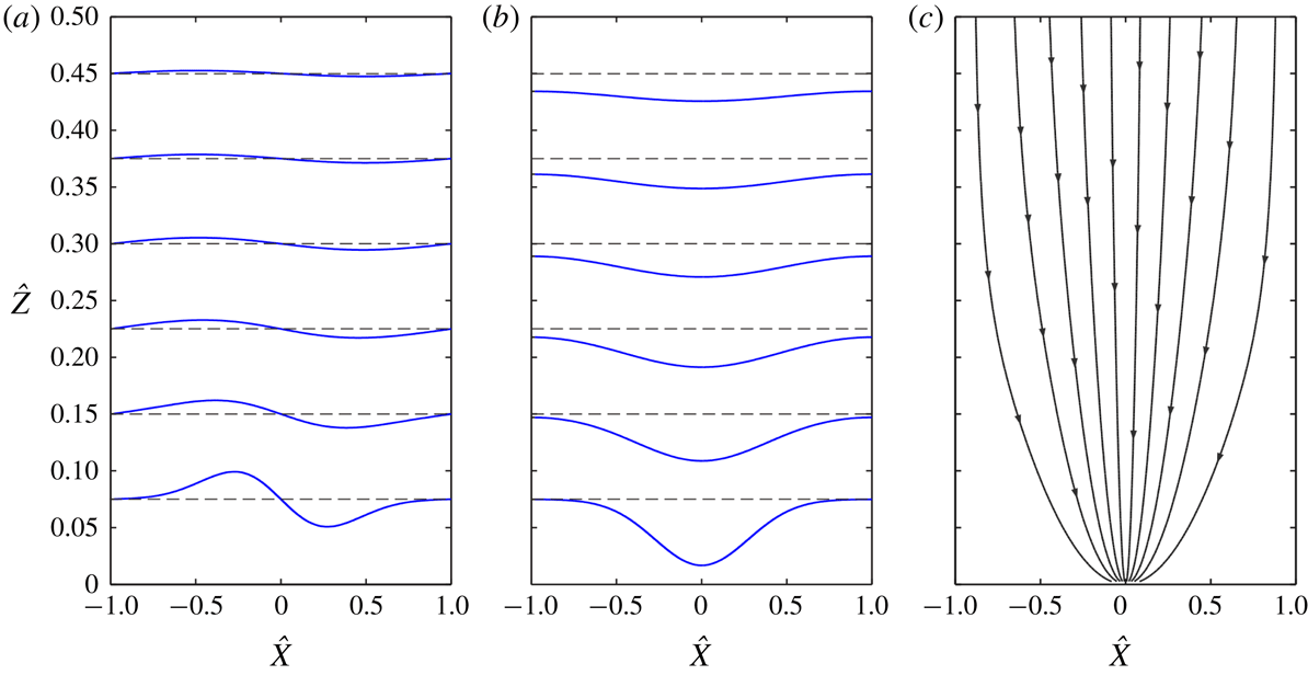
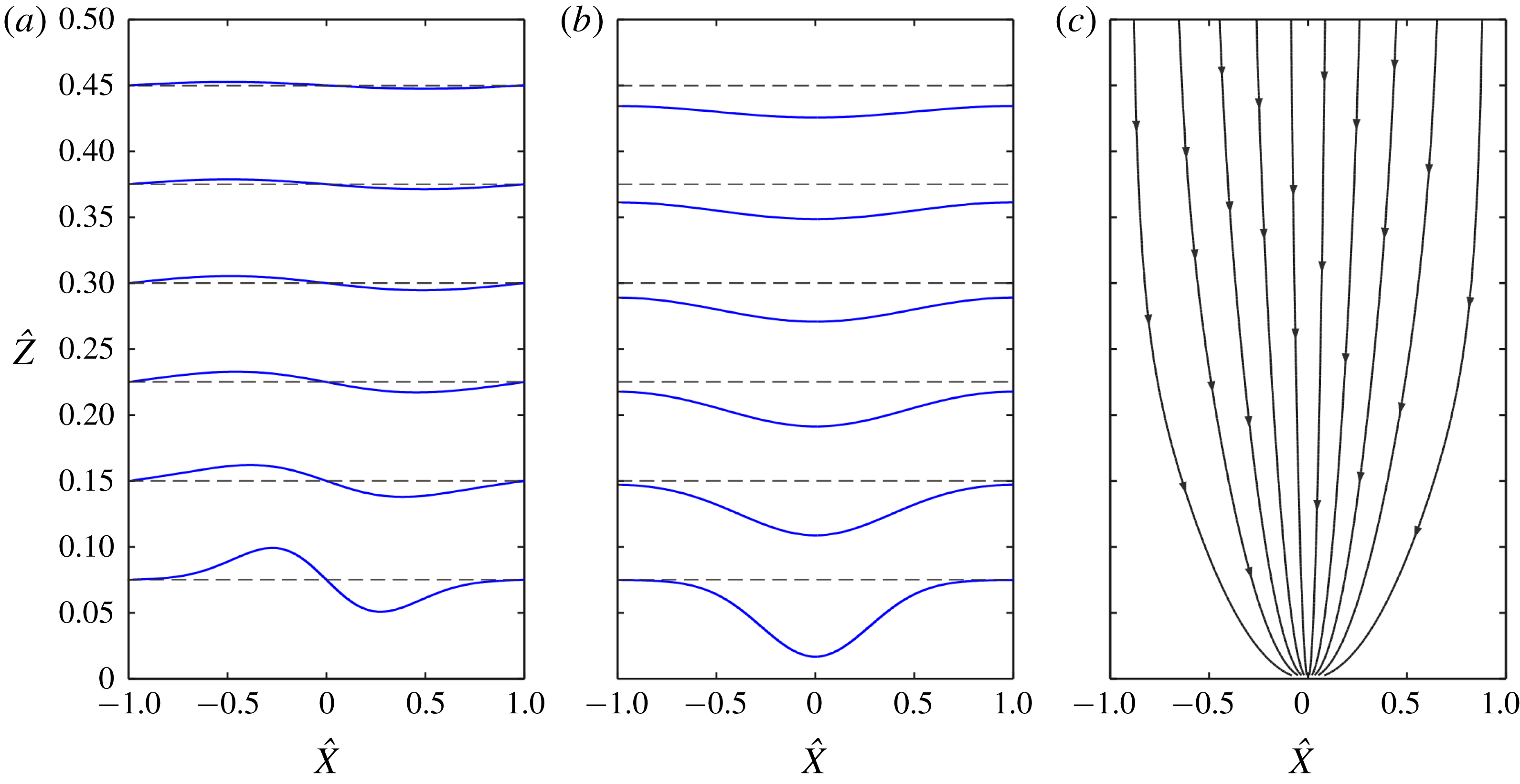
The resulting dimensionless solutions are illustrated in figure 2. Figure 2(a) shows spanwise profiles of horizontal velocity at different heights above the orifice. Figure 2(b) shows the corresponding profiles of vertical velocity. Finally figure 2(c) shows the streamlines
 $\hat{\unicode[STIX]{x1D6F9}}=$
constant for equally spaced values of the streamfunction. Near the orifice, flow is apparent only in the central region, but there is no sharp boundary between flowing and stationary regions. The diffusion solutions feature small non-zero motions even away from the central zone. Using the kinematic model, similar deep flow fields in silos have earlier been calculated by Nedderman & Tüzün (Reference Nedderman and Tüzün1979), using Fourier series, and by Choi et al. (Reference Choi, Kudrolli and Bazant2005) using numerical computations.
Solutions to the kinematic deep flow model: (a) spanwise profiles of horizontal velocity; (b) spanwise profiles of vertical velocity; (c) streamlines.
2.2 Shallow layer governing equations
To model surface avalanching (figure 3), we consider a distinct coordinate system
 $(x,z)$
tilted at the angle of repose
 $\unicode[STIX]{x1D6FC}$
, with origin at
 $(X,Z)=(-L/2,H(t))$
and descending with the granular free surface at speed
 ${\dot{H}}=-Q/L$
. The
 $x$
-axis of the coordinate system therefore coincides with the inclined profile (figure 3
a)
 $$\begin{eqnarray}\text{}\underline{Z}(X,t)=H(t)-(X+L/2)\tan \unicode[STIX]{x1D6FC}.\end{eqnarray}$$
Throughout this section, we assume the restricted domain
 $-L\leqslant X\leqslant 0$
, with mirror symmetry implied in case of a symmetric silo. In the inclined coordinate system, we define
 $\widetilde{z}(x,t)$
and
 ${\displaystyle\mathop{z}\limits_{{\sim}}}(x,t)$
to be the free surface and basal boundary of the avalanching layer. The depth of the avalanching layer is then given by
 $h(x,t)=\widetilde{z}-{\displaystyle\mathop{z}\limits_{{\sim}}}$
. We assume shallow flow,
 $h\ll L$
, and small relief
 $\widetilde{z}\ll L$
relative to profile
 $z=0$
inclined at the angle of repose. Consistent with these approximations, flow acceleration in the
 $z$
-direction will be neglected relative to acceleration in the downslope
 $x$
-direction. However both velocity components,
 $u(x,z,t)$
, in the
 $x$
-direction and
 $w(x,z,t)$
in the
 $z$
-direction, will intervene in the flow kinematics. Inspired from Liggett (Reference Liggett1994), and following Capart et al. (Reference Capart, Hung and Stark2015) and Hung et al. (Reference Hung, Stark and Capart2016), we use different lines above and below variables to denote values sampled at different locations:
 ${\displaystyle\mathop{\,\cdot \,}\limits_{{\sim}}}$
denotes a variable sampled along the basal boundary,
 $\tilde{\,\cdot \,}$
a variable sampled along the free surface and
 $\text{}\underline{\,\cdot \,}$
a variable sampled along the angle of repose profile (2.11). The overbar
 $\overline{\,\cdot \,}$
is reserved for quantities averaged over the depth
 $h$
.
Definition sketch of surface flow model: (a) overview; (b) local cutaway. The surface flow is depicted in a frame of reference descending with the free surface, in which the flow is approximately steady. In this frame of reference, the erosion flux across the basal interface exhibits a change of sign, from positive upstream to negative downstream, hence the apparent kink in (a).

Following Capart et al. (Reference Capart, Hung and Stark2015), we start from local equations and integrate them from
 ${\displaystyle\mathop{z}\limits_{{\sim}}}$
to
 $\widetilde{z}$
to obtain depth-integrated equations governing the avalanching layer. As for the deep flow, we assume incompressibility of the granular medium, hence the local continuity equation
 $$\begin{eqnarray}\frac{\unicode[STIX]{x2202}u}{\unicode[STIX]{x2202}x}+\frac{\unicode[STIX]{x2202}w}{\unicode[STIX]{x2202}z}=0.\end{eqnarray}$$
Variations of
 $u$
and
 $w$
in the transverse
 $y$
-direction are neglected, hence
 $u$
and
 $w$
coincide with the corresponding velocity components averaged over the gap thickness. Local balance of momentum in the
 $x$
-direction, on the other hand, yields the width-averaged equation of motion (Jop et al.
Reference Jop, Forterre and Pouliquen2007)
 $$\begin{eqnarray}\unicode[STIX]{x1D70C}\left(\frac{\unicode[STIX]{x2202}u}{\unicode[STIX]{x2202}t}+u\frac{\unicode[STIX]{x2202}u}{\unicode[STIX]{x2202}x}+w\frac{\unicode[STIX]{x2202}u}{\unicode[STIX]{x2202}z}\right)=\unicode[STIX]{x1D70C}g_{_{\Vert }}-\frac{\unicode[STIX]{x2202}p}{\unicode[STIX]{x2202}x}+\frac{\unicode[STIX]{x2202}\unicode[STIX]{x1D70F}}{\unicode[STIX]{x2202}z}-\frac{2\unicode[STIX]{x1D70F}_{W}}{B},\end{eqnarray}$$
where
 $\unicode[STIX]{x1D70C}=c_{S}\unicode[STIX]{x1D70C}_{S}$
is the mean density of the bulk phase, and
 $p=\unicode[STIX]{x1D70C}g_{_{\bot }}(\,\widetilde{z}-z)$
is the granular pressure, assumed lithostatic. Following Jop et al. (Reference Jop, Forterre and Pouliquen2005), the normal stresses are assumed to reduce to an isotropic pressure. For shallow flow (Liggett Reference Liggett1994), granular accelerations in the
 $z$
direction normal to the slope can be neglected, hence a lithostatic pressure balancing the weight of the grains above. In the same equation,
 $g_{_{\Vert }}=g\sin \unicode[STIX]{x1D6FC}$
and
 $g_{\bot }=g\cos \unicode[STIX]{x1D6FC}$
are the parallel and perpendicular components of the gravitational acceleration,
 $\unicode[STIX]{x1D70F}_{W}=\unicode[STIX]{x1D707}_{W}p$
is the shear stress along the side walls (with
 $\unicode[STIX]{x1D707}_{W}$
the wall friction coefficient) and
 $\unicode[STIX]{x1D70F}$
is the internal shear stress. For the latter, we assume the viscoplastic, dense granular flow rheology (da Cruz et al.
Reference da Cruz, Emam, Prochnow, Roux and Chevoir2005)
 $$\begin{eqnarray}\unicode[STIX]{x1D70F}=\unicode[STIX]{x1D707}_{0}p+\unicode[STIX]{x1D712}D(\unicode[STIX]{x1D70C}p)^{1/2}\dot{\unicode[STIX]{x1D6FE}},\end{eqnarray}$$
expressed as the sum of two components. The first, rate independent, is a plastic yield stress proportional to
 $p$
, with coefficient
 $\unicode[STIX]{x1D707}_{0}=\tan \unicode[STIX]{x1D6FC}$
. The second, rate dependent, is a viscous stress that varies linearly with the shear rate
 $\dot{\unicode[STIX]{x1D6FE}}=\unicode[STIX]{x2202}u/\unicode[STIX]{x2202}z$
, with effective viscosity
 $\unicode[STIX]{x1D712}D(\unicode[STIX]{x1D70C}p)^{1/2}$
dependent on grain diameter
 $D$
, granular pressure
 $p$
and dimensionless rheological coefficient
 $\unicode[STIX]{x1D712}$
. This is a linearized version of the
 $\unicode[STIX]{x1D707}(I)$
rheology proposed by Jop et al. (Reference Jop, Forterre and Pouliquen2005) and applied earlier to liquid–granular flows by Berzi & Jenkins (Reference Berzi and Jenkins2008). The nonlinear
 $\unicode[STIX]{x1D707}(I)$
rheology has earlier been applied to shallow granular flows over rigid beds by Gray & Edwards (Reference Gray and Edwards2014). The two rheological coefficient
 $\unicode[STIX]{x1D707}_{0}$
and
 $\unicode[STIX]{x1D712}$
will be determined in the next section by linearizing the nonlinear
 $\unicode[STIX]{x1D707}(I)$
rheology calibrated earlier by Jop et al. (Reference Jop, Forterre and Pouliquen2005) for the same granular material. Note that the constitutive relations for wall friction and internal shear stress are written assuming
 $u>u_{W}$
, and
 $\dot{\unicode[STIX]{x1D6FE}}>0$
. For steady uniform flow over a loose deposit of velocity (
 ${\displaystyle\mathop{u}\limits_{{\sim}}}$
,
 ${\displaystyle\mathop{w}\limits_{{\sim}}}$
), these equations are satisfied by the velocity profile (figure 3
b)
 $$\begin{eqnarray}u(\widehat{\unicode[STIX]{x1D702}})={\displaystyle\mathop{u}\limits_{{\sim}}}+(\overline{u}-{\displaystyle\mathop{u}\limits_{{\sim}}})({\textstyle \frac{7}{3}}-{\textstyle \frac{35}{6}}\widehat{\unicode[STIX]{x1D702}}^{3/2}+{\textstyle \frac{7}{2}}\widehat{\unicode[STIX]{x1D702}}^{5/2}),\end{eqnarray}$$
where
 $\widehat{\unicode[STIX]{x1D702}}=(\,\widetilde{z}-z)/h$
and
 $\overline{u}$
is the depth-averaged velocity (for a derivation, see Berzi & Jenkins (Reference Berzi and Jenkins2008)). As discussed in Capart et al. (Reference Capart, Hung and Stark2015), experiments exhibit some deviations from the profile (2.15) even for equilibrium flows. For unsteady, non-uniform flows, moreover, the velocity profile is expected to deviate from its equilibrium shape. As long as such deviations are small, however, integrals over depth based on the profile (2.15) should furnish a good approximation, and provide a simple way to close depth-integrated equations. Because the corresponding shear rate at the base
 ${\displaystyle\mathop{\{}\limits_{{\sim}}}=\unicode[STIX]{x2202}u/\unicode[STIX]{x2202}z({\displaystyle\mathop{z}\limits_{{\sim}}})$
is equal to zero, note that this profile is appropriate only for flows over erodible beds, when the basal interface can be assumed to coincide with the yield locus. For flows over rigid beds, say over rock, a finite shear rate at the base would be expected, and the base elevation prescribed, instead of the present case with zero basal shear rate and a basal elevation set by the flow itself. Likewise, the description would not apply for granular flows over deposits composed of a different type of grains. When assumptions are met, the velocity profile
 $u(x,z,t)$
at a given coordinate
 $x$
and time
 $t$
can be calculated using (2.15) from
 $\widetilde{z}(x,t)$
,
 $h(x,t)$
,
 $\overline{u}(x,t)$
and
 ${\displaystyle\mathop{u}\limits_{{\sim}}}(x,t)$
. The corresponding streamfunction, likewise, can be calculated from
 $$\begin{eqnarray}\unicode[STIX]{x1D713}(\hat{\unicode[STIX]{x1D702}})=\widetilde{\unicode[STIX]{x1D713}}-h{\displaystyle\mathop{u}\limits_{{\sim}}}\hat{\unicode[STIX]{x1D702}}-h(\overline{u}-{\displaystyle\mathop{u}\limits_{{\sim}}})({\textstyle \frac{7}{3}}\hat{\unicode[STIX]{x1D702}}-{\textstyle \frac{7}{3}}\hat{\unicode[STIX]{x1D702}}^{5/2}+\hat{\unicode[STIX]{x1D702}}^{7/2}),\end{eqnarray}$$
where
 $\unicode[STIX]{x1D713}$
satisfies
 $\unicode[STIX]{x2202}\unicode[STIX]{x1D713}/\unicode[STIX]{x2202}z=u$
,
 $\unicode[STIX]{x2202}\unicode[STIX]{x1D713}/\unicode[STIX]{x2202}x=-w$
, and such that
 $$\begin{eqnarray}\widetilde{\unicode[STIX]{x1D713}}-{\displaystyle\mathop{\unicode[STIX]{x1D713}}\limits_{{\sim}}}=h\overline{u}.\end{eqnarray}$$
To obtain unsteady, non-uniform governing equations for the avalanching layer, we first integrate (2.12) and apply the Leibniz integral rule to get
 $$\begin{eqnarray}\int _{{\displaystyle\mathop{z}\limits_{{\sim}}}}^{\widetilde{z}}\left(\frac{\unicode[STIX]{x2202}u}{\unicode[STIX]{x2202}x}+\frac{\unicode[STIX]{x2202}w}{\unicode[STIX]{x2202}z}\right)\text{d}z=\frac{\unicode[STIX]{x2202}(h\overline{u})}{\unicode[STIX]{x2202}x}-\widetilde{u}\frac{\unicode[STIX]{x2202}\widetilde{z}}{\unicode[STIX]{x2202}x}+{\displaystyle\mathop{u}\limits_{{\sim}}}\frac{\unicode[STIX]{x2202}{\displaystyle\mathop{z}\limits_{{\sim}}}}{\unicode[STIX]{x2202}x}+\widetilde{w}-{\displaystyle\mathop{w}\limits_{{\sim}}}=0,\end{eqnarray}$$
where
 $q=h\overline{u}=\int _{{\displaystyle\mathop{z}\limits_{{\sim}}}}^{\widetilde{z}}u\,\text{d}z$
. This can be further worked out using the kinematic boundary condition along the free surface,
 $$\begin{eqnarray}\frac{\unicode[STIX]{x2202}\widetilde{z}}{\unicode[STIX]{x2202}t}+\widetilde{u}\frac{\unicode[STIX]{x2202}\widetilde{z}}{\unicode[STIX]{x2202}x}=\widetilde{w},\end{eqnarray}$$
and the definition
 $h=\widetilde{z}-{\displaystyle\mathop{z}\limits_{{\sim}}}$
to obtain the depth-integrated continuity equation
 $$\begin{eqnarray}\frac{\unicode[STIX]{x2202}h}{\unicode[STIX]{x2202}t}+\frac{\unicode[STIX]{x2202}(h\overline{u})}{\unicode[STIX]{x2202}x}=e={\displaystyle\mathop{w}\limits_{{\sim}}}-{\displaystyle\mathop{u}\limits_{{\sim}}}\frac{\unicode[STIX]{x2202}{\displaystyle\mathop{z}\limits_{{\sim}}}}{\unicode[STIX]{x2202}x}-\frac{\unicode[STIX]{x2202}{\displaystyle\mathop{z}\limits_{{\sim}}}}{\unicode[STIX]{x2202}t},\end{eqnarray}$$
where
 $e(x,t)$
is the erosion or entrainment rate, or rate of granular volume transfer across the basal interface
 ${\displaystyle\mathop{z}\limits_{{\sim}}}(x,t)$
and into the avalanching layer. This rate is defined as the deviation from volume conservation of the layer, expressed by the left-hand side. Likewise, the local equation of motion (2.13) can be integrated over depth to obtain the depth-integrated momentum equation
 $$\begin{eqnarray}\frac{\unicode[STIX]{x2202}}{\unicode[STIX]{x2202}t}(h\overline{u})+\frac{\unicode[STIX]{x2202}}{\unicode[STIX]{x2202}x}(h\,\overline{u^{2}})=e{\displaystyle\mathop{u}\limits_{{\sim}}}+g_{_{\Vert }}h-g_{_{\bot }}h\frac{\unicode[STIX]{x2202}\widetilde{z}}{\unicode[STIX]{x2202}x}-\frac{1}{\unicode[STIX]{x1D70C}}{\displaystyle\mathop{\unicode[STIX]{x1D70F}}\limits_{{\sim}}}-\frac{2}{\unicode[STIX]{x1D70C}B}h\overline{\unicode[STIX]{x1D70F}}_{W}.\end{eqnarray}$$
Assuming
 ${\displaystyle\mathop{u}\limits_{{\sim}}}(x,t)$
,
 ${\displaystyle\mathop{w}\limits_{{\sim}}}(x,t)$
to be otherwise given, we must solve for three evolving profiles
 $h(x,t)$
,
 $\widetilde{z}(x,t)$
and
 $\overline{u}(x,t)$
. We therefore supplement (2.20) and (2.21) with an additional equation expressing the balance of depth-integrated kinetic energy (Capart et al.
Reference Capart, Hung and Stark2015; Hung et al.
Reference Hung, Stark and Capart2016). This is obtained by integrating over depth the product of (2.13) with velocity
 $u(x,z,t)$
, yielding
 $$\begin{eqnarray}\frac{\unicode[STIX]{x2202}}{\unicode[STIX]{x2202}t}\left(\frac{h\,\overline{u^{2}}}{2}\right)+\frac{\unicode[STIX]{x2202}}{\unicode[STIX]{x2202}x}\left(\frac{h\,\overline{u^{3}}}{2}\right)=\frac{e{\displaystyle\mathop{u}\limits_{{\sim}}}^{2}}{2}+g_{_{\Vert }}h\overline{u}-g_{_{\bot }}h\overline{u}\frac{\unicode[STIX]{x2202}\widetilde{z}}{\unicode[STIX]{x2202}x}-{\displaystyle\mathop{\unicode[STIX]{x1D70F}}\limits_{{\sim}}}{\displaystyle\mathop{u}\limits_{{\sim}}}-\frac{1}{\unicode[STIX]{x1D70C}}h\,\overline{\unicode[STIX]{x1D70F}\dot{\unicode[STIX]{x1D6FE}}}-\frac{2}{\unicode[STIX]{x1D70C}B}h\,\overline{\unicode[STIX]{x1D70F}_{W}u}.\end{eqnarray}$$
In this equation, the next-to-last and last terms represent dissipation by granular contacts inside the avalanching layer and dissipation by friction along the walls, respectively. Equations (2.20)–(2.22) represent a generalization of the equations derived in Capart et al. (Reference Capart, Hung and Stark2015) for the case of stationary deposits (
 ${\displaystyle\mathop{u}\limits_{{\sim}}}={\displaystyle\mathop{w}\limits_{{\sim}}}=0$
). We now specialize them to the problem of avalanching flows over loose deposits undergoing uneven subsidence due to silo discharge. Ideally, we would wish to match the velocity at the base of the avalanching layer with the deep flow velocity along the same curve, i.e. let
 $({\displaystyle\mathop{u}\limits_{{\sim}}},{\displaystyle\mathop{w}\limits_{{\sim}}})=({\displaystyle\mathop{u}\limits_{{\sim}}}_{0},{\displaystyle\mathop{w}\limits_{{\sim}}}_{0})$
. The precise shape of the basal interface
 ${\displaystyle\mathop{z}\limits_{{\sim}}}(x,z,t)$
, however, is not known in advance. As in linearized groundwater seepage problems (see e.g. Ni & Capart Reference Ni and Capart2006), therefore, we choose instead to apply kinematic matching to the approximate basal interface given by
 $\text{}\underline{Z}(X,t)$
. This corresponds to the linear profile (2.11), inclined at the angle of repose. We therefore approximate
 $$\begin{eqnarray}\displaystyle & \displaystyle {\displaystyle\mathop{u}\limits_{{\sim}}}\approx \text{}\underline{u}_{0}=\text{}\underline{U\!}_{\,0}\cos \unicode[STIX]{x1D6FC}-(\text{}\underline{W\!}_{\,0}-{\dot{H}})\sin \unicode[STIX]{x1D6FC}, & \displaystyle\end{eqnarray}$$
 $$\begin{eqnarray}\displaystyle & \displaystyle {\displaystyle\mathop{w}\limits_{{\sim}}}\approx \text{}\underline{w}_{0}=\text{}\underline{U\!}_{\,0}\sin \unicode[STIX]{x1D6FC}+(\text{}\underline{W\!}_{\,0}-{\dot{H}})\cos \unicode[STIX]{x1D6FC}, & \displaystyle\end{eqnarray}$$
where velocities in the upright, stationary silo frame of reference are converted to the tilted frame of reference descending at constant speed
 ${\dot{H}}$
. Likewise we approximate
 $$\begin{eqnarray}{\displaystyle\mathop{w}\limits_{{\sim}}}+{\displaystyle\mathop{u}\limits_{{\sim}}}\frac{\unicode[STIX]{x2202}{\displaystyle\mathop{z}\limits_{{\sim}}}}{\unicode[STIX]{x2202}x}\approx \text{}\underline{w}_{0}+\text{}\underline{u}_{0}\frac{\unicode[STIX]{x2202}\text{}\underline{z}}{\unicode[STIX]{x2202}x}=\text{}\underline{w}_{0}.\end{eqnarray}$$
In terms of the streamfunction, equivalently, we let
 $$\begin{eqnarray}{\displaystyle\mathop{\unicode[STIX]{x1D713}}\limits_{{\sim}}}\approx \text{}\underline{\unicode[STIX]{x1D713}\!}_{\,0}=\text{}\underline{\unicode[STIX]{x1D6F9}\!}_{\,0}+{\dot{H}}\text{}\underline{X},\end{eqnarray}$$
where
 $\text{}\underline{\unicode[STIX]{x1D6F9}\!}_{\,0}$
is the streamfunction (2.9) sampled along
 $(\text{}\underline{X},\text{}\underline{Z})(x,t)=(-L/2+x\cos \unicode[STIX]{x1D6FC},H(t)-x\sin \unicode[STIX]{x1D6FC})$
. The solutions presented below are obtained by applying the matching condition at this known, but approximate interface position
 $\text{}\underline{Z}(X,t)$
. We could instead proceed by iterations, applying the matching condition again at each step to the interface location calculated from the previous step. Because the deep flow varies gradually with height above orifice, however, the error of the approximate solution with respect to the converged iterative solution is small, hence we prefer the simpler approach. With this approximation, the depth-integrated continuity equation becomes
 $$\begin{eqnarray}\frac{\unicode[STIX]{x2202}\widetilde{z}}{\unicode[STIX]{x2202}t}+\frac{\unicode[STIX]{x2202}(h\overline{u})}{\unicode[STIX]{x2202}x}=\text{}\underline{w}_{0}.\end{eqnarray}$$
For quasi-steady flow, the dominant balance is between the second and third terms, hence
 $\text{}\underline{w}_{0}\sim h\overline{u}/L$
. For shallow flow the ratio
 $h/L=\unicode[STIX]{x1D716}$
is small, thus the deep flow velocity components
 $\text{}\underline{u_{0}}\sim \text{}\underline{w_{0}}\sim \unicode[STIX]{x1D716}\overline{u}$
are one order of magnitude smaller than the depth-averaged avalanche velocity
 $\overline{u}$
. Terms associated with the basal velocity
 ${\displaystyle\mathop{u}\limits_{{\sim}}}\approx \text{}\underline{u}_{0}$
can therefore be neglected in the momentum and kinetic energy equations (2.21) and (2.22). Likewise we can set
 ${\displaystyle\mathop{u}\limits_{{\sim}}}=0$
in (2.15). With these simplifications, equations (2.21)–(2.22) governing the dynamics of the avalanching layer become
 $$\begin{eqnarray}\displaystyle & \displaystyle \frac{\unicode[STIX]{x2202}}{\unicode[STIX]{x2202}t}(h\overline{u})+\frac{\unicode[STIX]{x2202}}{\unicode[STIX]{x2202}x}\left(\frac{77}{48}h\overline{u}^{2}\right)=-g_{_{\bot }}h\frac{\unicode[STIX]{x2202}\widetilde{z}}{\unicode[STIX]{x2202}x}-\frac{\unicode[STIX]{x1D707}_{W}}{B}g_{_{\bot }}h^{2}, & \displaystyle\end{eqnarray}$$
 $$\begin{eqnarray}\displaystyle & \displaystyle \frac{\unicode[STIX]{x2202}}{\unicode[STIX]{x2202}t}\left(\frac{77}{96}h\overline{u}^{2}\right)+\frac{\unicode[STIX]{x2202}}{\unicode[STIX]{x2202}x}(\unicode[STIX]{x1D705}h\overline{u}^{3})=-g_{_{\bot }}h\overline{u}\frac{\unicode[STIX]{x2202}\widetilde{z}}{\unicode[STIX]{x2202}x}-\frac{35}{9}\unicode[STIX]{x1D712}Dg_{\bot }^{1/2}\frac{\overline{u}^{2}}{h^{1/2}}-\frac{5}{9}\frac{\unicode[STIX]{x1D707}_{W}}{B}g_{_{\bot }}h^{2}\overline{u}, & \displaystyle\end{eqnarray}$$
where
 $\unicode[STIX]{x1D705}=342853/233376\approx 1.469$
, and where the depth-integrated terms
 $\overline{u^{2}}$
and
 $\overline{u^{3}}$
were integrated using profile (2.15) with
 ${\displaystyle\mathop{u}\limits_{{\sim}}}=0$
. The last two terms of (2.29), representing energy dissipation, are obtained by integration of the corresponding terms
 $\overline{\unicode[STIX]{x1D70F}\dot{\unicode[STIX]{x1D6FE}}}$
and
 $\overline{\unicode[STIX]{x1D70F}_{W}u}$
in (2.22), using profile (2.15) and the rheology (2.14). The next-to-last term of (2.29) is thus controlled by the rheology coefficient
 $\unicode[STIX]{x1D712}$
that determines the effective viscosity. After simplification, equations (2.28) and (2.29) are identical to the momentum and kinetic energy equations derived earlier in Capart et al. (Reference Capart, Hung and Stark2015). Together with (2.27) they form a closed set of governing equations for profiles
 $\widetilde{z}(x,t)$
,
 $h(x,t)$
and
 $\overline{u}(x,t)$
, driven by the deep flow velocities
 $\text{}\underline{U\!}_{\,0}(x,t)$
and
 $\text{}\underline{W\!}_{\,0}(x,t)$
. These in turn can be estimated using the kinematic model described in the previous section. While these unsteady equations could in principle be solved numerically to describe the transient response, here we consider only the quasi-steady response obtained by neglecting the time derivatives in (2.27)–(2.29). The semi-analytical approach used to construct solutions for this case is described in the next sub-section.
2.3 Quasi-steady avalanching solutions
For quasi-steady flow, the continuity equation (2.27) reduces to
 $$\begin{eqnarray}\frac{\unicode[STIX]{x2202}q}{\unicode[STIX]{x2202}x}=\text{}\underline{w}_{0}=-\frac{\unicode[STIX]{x2202}\text{}\underline{\unicode[STIX]{x1D713}\!}_{\,0}}{\unicode[STIX]{x2202}x},\end{eqnarray}$$
where
 $q=h\overline{u}$
is the depth-integrated granular discharge of the avalanching layer. Integration with boundary conditions
 $q=0$
,
 $\text{}\underline{\unicode[STIX]{x1D713}\!}_{\,0}=0$
at
 $x=L/(2\cos \unicode[STIX]{x1D6FC})$
then yields
 $$\begin{eqnarray}q(x,t)=-\text{}\underline{\unicode[STIX]{x1D713}\!}_{\,0}(x,t),\end{eqnarray}$$
such that
 $q=0$
is also automatically satisfied at
 $x=-L/(2\cos \unicode[STIX]{x1D6FC})$
. As expected, it follows from (2.17) and (2.31) that
 $\widetilde{\unicode[STIX]{x1D713}}=0$
, i.e. the quasi-steady free surface coincides with the zero streamline. For quasi-steady flow, the downslope distribution of the avalanching discharge
 $q(x,t)$
is therefore fully known, including its maximum value
 $q_{max}(t)$
at any given time
 $t$
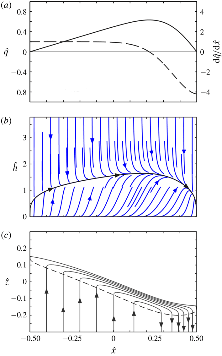
during the descent. An example is illustrated in figure 4(a). Hereafter, we drop the explicit time dependence, but note that the evolving height
 $H(t)$
of the avalanching layer during its descent will affect its discharge profile
 $q(x)$
.
Dynamic model solution for the avalanching layer: (a) imposed spanwise profile of normal to slope velocity
 ${\hat{w}}_{0}=\text{d}\hat{q}/\text{d}\hat{x}$
(dashed line) and the resulting avalanching discharge
 $\hat{q}(\hat{x})$
(continuous line); (b) dimensionless phase diagram
 $(\hat{x},{\hat{h}})$
with the solution curve
 ${\hat{h}}(\hat{x})$
in black; (c) basal interface (dashed line) and streamlines (continuous lines) in the frame of reference descending with the free surface.

To solve the momentum and kinetic energy equations (2.28) and (2.29) subject to the known discharge profile
 $q(x)$
, we substitute
 $\overline{u}=q/h$
and introduce the dimensionless variables
 $\hat{x}=x/(L/\cos \unicode[STIX]{x1D6FC})$
,
 $\hat{q}=q/Q$
,
 ${\hat{h}}=h/h_{a}$
,
 ${\hat{S}}=(-\unicode[STIX]{x2202}\widetilde{z}/\unicode[STIX]{x2202}x)/S_{a}$
, where
 $$\begin{eqnarray}h_{a}=\left(\frac{\unicode[STIX]{x1D712}DQ}{g_{\bot }^{1/2}\unicode[STIX]{x1D707}_{W}/B}\right)^{2/7}\quad \text{and}\quad S_{a}=\frac{\unicode[STIX]{x1D707}_{W}}{B}h_{a}\end{eqnarray}$$
are the characteristic depth and excess surface inclination associated with equilibrium avalanching flow (Hung et al.
Reference Hung, Stark and Capart2016). At equilibrium, the flow is paced (via the rheological coefficient
 $\unicode[STIX]{x1D712}$
) by the rate-dependent term of the dense granular flow rheology (2.14). Translated to dimensionless form, (2.28) and (2.29) become
 $$\begin{eqnarray}\displaystyle & \displaystyle \hat{Q}^{8/7}\frac{\unicode[STIX]{x2202}}{\unicode[STIX]{x2202}\hat{x}}\left(\frac{77}{48}\frac{\hat{q}^{2}}{{\hat{h}}}\right)={\hat{h}}{\hat{S}}-{\hat{h}}^{2}, & \displaystyle\end{eqnarray}$$
 $$\begin{eqnarray}\displaystyle & \displaystyle \hat{Q}^{8/7}\frac{\unicode[STIX]{x2202}}{\unicode[STIX]{x2202}\hat{x}}\left(\frac{\unicode[STIX]{x1D705}\hat{q}^{3}}{{\hat{h}}^{2}}\right)=\hat{q}{\hat{S}}-\frac{35}{9}\frac{\hat{q}^{2}}{{\hat{h}}^{5/2}}-\frac{5}{9}{\hat{h}}\hat{q}, & \displaystyle\end{eqnarray}$$
where
 $\hat{Q}$
is the dimensionless silo discharge
 $$\begin{eqnarray}\hat{Q}=\frac{Q}{(\unicode[STIX]{x1D707}_{W}/B)^{1/8}g_{\bot }^{1/2}(\unicode[STIX]{x1D712}D)^{3/4}(L/\cos \unicode[STIX]{x1D6FC})^{7/8}}.\end{eqnarray}$$
An equivalent dimensionless number, found to control avalanching behaviour in rotating drums, was given the name entrainment number by Hung et al. (Reference Hung, Stark and Capart2016). It can be seen from (2.33) and (2.34) that this number controls the strength of the left-hand side flux divergence terms associated with convective inertia. For low
 $\hat{Q}$
, the avalanching layer is locally in equilibrium and its behaviour is dominated by the dense granular flow rheology. In the inertialess limit
 $\hat{Q}\rightarrow 0$
, in particular, the flux divergence terms disappear, and the solution is simply
 $$\begin{eqnarray}{\hat{h}}(\hat{x})=({\textstyle \frac{35}{4}}\hat{q}(\hat{x}))^{2/7},\quad {\hat{S}}(\hat{x})={\hat{h}}(\hat{x}).\end{eqnarray}$$
For high
 $\hat{Q}$
, in contrast, inertia effects dominate and take the flow far from local equilibrium (Hung et al.
Reference Hung, Stark and Capart2016). For intermediate
 $\hat{Q}$
, both inertia and rheology intervene. The equations in that case can be solved by eliminating
 ${\hat{S}}$
between (2.33) and (2.34), yielding for
 ${\hat{h}}$
the ordinary differential equation of the first order
 $$\begin{eqnarray}\frac{\text{d}{\hat{h}}}{\text{d}\hat{x}}=\frac{{\textstyle \frac{35}{9}}{\hat{h}}^{1/2}\hat{q}-{\textstyle \frac{4}{9}}{\hat{h}}^{4}+\hat{Q}^{8/7}(3\unicode[STIX]{x1D705}-{\textstyle \frac{77}{24}}){\hat{h}}\hat{q}\,\text{d}\hat{q}/\text{d}\hat{x}}{\hat{Q}^{8/7}(2\unicode[STIX]{x1D705}-{\textstyle \frac{77}{48}})\hat{q}^{2}}.\end{eqnarray}$$
Starting from
 ${\hat{h}}(-1/2)=0$
at the upstream boundary, this nonlinear equation can be integrated numerically in the phase plane
 $(\hat{x},{\hat{h}})$
to obtain the solution curve
 ${\hat{h}}(\hat{x})$
(figure 4
b). Because the solution has vertical tangents at end points
 $\hat{x}=\pm 1/2$
, we integrate using discrete steps of constant distance
 $\text{d}\hat{\unicode[STIX]{x1D709}}=(\text{d}\hat{x}^{2}+\text{d}{\hat{h}}^{2})^{1/2}$
rather than constant intervals
 $\text{d}\hat{x}$
. Next, we deduce the excess inclination profile
 ${\hat{S}}$
by substituting the solution to (2.37) back into (2.33). Finally, the free surface profile
 $\hat{\widetilde{z}}(\hat{x})=\widetilde{z}/(S_{a}L/\cos \unicode[STIX]{x1D6FC})$
is determined by integrating
 $\text{d}\hat{\widetilde{z}}/\text{d}\hat{x}=-{\hat{S}}$
numerically subject to the integral condition
 $\int _{-1/2}^{1/2}\hat{\widetilde{z}}\text{d}\hat{x}=0$
. Results are plotted in figure 4(c), together with the streamlines calculated from (2.16). For the experiments below, the dimensionless silo discharge
 $\hat{Q}$
takes relatively low values, hence the inertialess solution (2.36) provides a good approximation to the full solution of (2.37). Because the basal forcing term and discharge distribution
 $\hat{q}(\hat{x})$
gradually evolve as the avalanching layer descends down the silo, note that solutions must be calculated anew for each time at which a snapshot of the flow is desired.
3 Experiments
The experiments were performed at the granular flow laboratory of IUSTI, Aix-Marseille University, using the set-up shown in figure 5. The rectangular silo is composed of parallel glass walls separated by wooden strips, planed to uniform thickness and sandwiched between the glass plates along the perimeter. By switching between different sets of wooden strips, three gap thicknesses
 $B_{1}=3.5~\text{mm}$
,
 $B_{2}=5~\text{mm}$
and
 $B_{3}=7~\text{mm}$
were investigated. To one side, wood pieces with mitred edges were used to control the orifice opening in the range 6 mm to 11 mm, yielding mass flowrates in the range
 ${\dot{m}}=3$
–
 $12~\text{g}~\text{s}^{-1}$
, as measured using a scale collecting the silo efflux. The lower edge of the orifice was set at a fixed height of 20 mm above the silo floor, and taken as origin
 $(X,Z)=(0,0)$
of the coordinate system. The internal silo chamber had spanwise width
 $L=60~\text{mm}$
and maximum depth
 $H_{max}=600~\text{mm}$
.
Experimental set-up: (a) schematic; (b) overview; (c) close-up showing the side orifice of the adjustable opening.

Slightly polydisperse glass spheres were used as granular material. Two different sphere sizes were tested, having diameters
 $D_{1}=0.5~\text{mm}$
and
 $D_{2}=0.76~\text{mm}$
. The
 $D_{1}$
spheres were drawn from a batch used in previous experiments, for which the following properties were determined in earlier work (Jop et al.
Reference Jop, Forterre and Pouliquen2005, Reference Jop, Forterre and Pouliquen2007): density
 $\unicode[STIX]{x1D70C}_{S}=2450~\text{kg}~\text{m}^{-3}$
, sphere–wall friction coefficient
 $\unicode[STIX]{x1D707}_{W}=\tan (13.1^{\circ })$
and parameters
 $\unicode[STIX]{x1D707}_{s}=\tan (20.9^{\circ })$
,
 $\unicode[STIX]{x1D707}_{2}=\tan (32.76^{\circ })$
and
 $I_{0}=0.279$
in the nonlinear
 $\unicode[STIX]{x1D707}(I)$
rheology
 $$\begin{eqnarray}\unicode[STIX]{x1D707}=\frac{\unicode[STIX]{x1D70F}}{\unicode[STIX]{x1D70E}}=\unicode[STIX]{x1D707}_{s}+\frac{\unicode[STIX]{x1D707}_{2}-\unicode[STIX]{x1D707}_{s}}{I_{0}/I+1},\end{eqnarray}$$
where
 $I=\dot{\unicode[STIX]{x1D6FE}}D/(p/\unicode[STIX]{x1D70C}_{S})^{1/2}$
is the inertia number. Provided that
 $I$
is not too large, this nonlinear relation between
 $\unicode[STIX]{x1D707}$
an
 $I$
can be linearized by Taylor expansion around
 $I=0$
. This yields for the coefficients of our assumed linear rheology (2.14) the values
 $\unicode[STIX]{x1D707}_{0}=\unicode[STIX]{x1D707}_{s}=0.38$
and
 $\unicode[STIX]{x1D712}=(\unicode[STIX]{x1D707}_{2}-\unicode[STIX]{x1D707}_{s})/(I_{0}c_{0}^{1/2})=1.2$
, where
 $c_{0}=0.6$
is the estimated granular volume fraction. These values of
 $\unicode[STIX]{x1D707}_{0}$
and
 $\unicode[STIX]{x1D712}$
are used without adjustment for all the comparisons between theory and experiment presented below. Based on the theory described in the previous section, we can estimate as follows the range of inertia numbers encountered in the present experiments. Using the theoretical velocity profile (2.15), first, the inertia number averaged over the depth of the avalanching layer is given by
 $$\begin{eqnarray}\overline{I}=\frac{35}{8}\frac{\overline{u}D}{(c_{0}g_{_{\bot }}h^{3})^{1/2}}.\end{eqnarray}$$
Using the approximation (2.36) and adopting the silo discharge
 $Q$
as an upper bound on the avalanching discharge
 $q$
, next, a maximum depth-averaged inertia number for each experiment can be obtained from
 $$\begin{eqnarray}\overline{I}_{max}=\frac{1}{2}\left(\frac{35}{4}\right)^{2/7}\frac{QD}{(c_{0}g_{_{\bot }}h_{a}^{5})^{1/2}}.\end{eqnarray}$$
The different conditions tested are listed in table 1.
Experimental conditions for the different runs.

Measurements were acquired using a Photron high-speed camera of resolution 640 by 640 pixels operated at frame rates in the range 250–500 frames per second. To maximize both the resolution and coverage of the footage acquired for each experiment, the silo was mounted on a motorized track allowing it to rise at constant speed
 $V\approx Q/L$
relative to the camera. In this fashion, the camera could zoom in on an observation window of width
 $L$
, within which the descending avalanching layer was nearly stationary. The lower part of the window, moreover, could scan the undisturbed deep flow, travelling past different regions of the deep flow as the silo moved relative to the camera. In one single experiment, therefore, the camera can record the deep flow over a height greater than the observation window, and capture the avalanching layer at different stages of its descent relative to the silo. Lighting was provided by a high-intensity LED, giving a point-like source of illumination that produced sharp highlights near the centres of the spheres, facilitating their capture and tracking.
Experiments were started with the silo filled up almost to maximum depth, with a level free surface. An initial transient was therefore needed to deform the free surface from its horizontal initial state to its tilted avalanching state. The time needed for a discharge
 $q\sim Q$
to resorb the corresponding triangular area
 $A=\tan \unicode[STIX]{x1D6FC}L^{2}/2$
is approximately
 $T=A/Q\sim L^{2}/Q$
. Over this time, the surface has descended by
 $\unicode[STIX]{x0394}H=-{\dot{H}}T\sim QT/L=L$
. To avoid this initial transient, measurements were therefore acquired only after an initial drawdown
 $\unicode[STIX]{x0394}H$
of at least 8 times the silo width
 $L$
. For this reason, the silo was designed to be twice as high as the target observation domain.
Particle tracking velocimetry was performed using the methods of Capart, Young & Zech (Reference Capart, Young and Zech2002), upgraded to take into account path regularity when matching particles from one frame to the next. For each experiment, of the order of
 $10^{8}$
velocity vectors were acquired. Averaging over multiple frames was conducted by binning vectors into non-overlapping Cartesian mesh cells, using distinct frames of reference for the deep flow and for the avalanching layer. For the deep flow, stationarity in the silo frame of reference was assumed to average vectors from the lower part of the window using a mesh of coordinates
 $(X,Z)$
. For the avalanching layer, averaging was performed in the descending frame of reference
 $(X,Z-{\dot{H}}t)$
, over time intervals of shorter duration to capture different stages of the layer evolution during its descent. During each experiment, an electronic scale was also used to monitor the mass outflow from the silo. Flow fields acquired in this fashion are illustrated in figure 6, and compared to long exposure images acquired with the silo moving or held stationary with respect to the camera.
Particle tracking velocimetry (PTV) process applied to run 3: (a) long exposure image for silo moving relative to the camera; (b) colour map of the measured magnitude of the granular velocity, averaged over 250 images; (c) reconstructed colour map of the deep granular velocity field, in the silo frame of reference; (d) composite long exposure image of the deep silo flow, with the silo held stationary with respect to the camera. In (a), the coloured lines illustrate the control volumes used to derive (4.2). In (b), the region below the dashed line was assumed unaffected by surface avalanching, yielding the measurements used to produce the deep flow map (c).

As a check on the PTV measurements and some of the assumptions of the theory, the mass flow rates
 ${\dot{m}}$
estimated by weighting the collected efflux can be compared with mass flow rates
 $c_{0}\unicode[STIX]{x1D70C}_{S}BQ$
estimated from particle tracking velocimetry, where
 $Q=-L\overline{W}_{0}$
is the volume flow rate per unit width and
 $\overline{W}_{0}$
is the mean downward velocity of the grains averaged from 12 cross-sections at different heights of the measured deep flow field. Values of both
 ${\dot{m}}$
and
 $Q$
are listed in table 1. The PTV values underestimate the collected efflux by up to 20 %, for the smaller grains, and by up to 10 % for the larger grains. This discrepancy indicates that the granular velocities measured by PTV along the tank front wall are somewhat slower than the granular velocities averaged over the gap thickness and associated with the bulk efflux. Since the discrepancy is not large, however, it appears reasonable to assume for simplicity that the flow is two-dimensional in character.
Qualitatively different avalanching flow pattern observed in silo of large gap thickness (
 $B=7~\text{mm}$
, run 7): (a) long exposure image; (b) colour map of velocity magnitude.

Reflecting the crucial role of wall friction (Jop et al.
Reference Jop, Forterre and Pouliquen2005), the silo gap thickness was found to exert a significant influence on the observed avalanching flow patterns. For small to medium gap thickness (
 $B=3.5$
and 5 mm), shallow avalanching layers are obtained, with lenticular shapes that span the entire silo width
 $L$
(figure 6). The resulting flow pattern (figure 6
b) is qualitatively similar to the flow field expected from the theory (see figure 4
c). The largest gap thickness tested, however
 $(B=7~\text{mm})$
, produces deep avalanching layers with slow velocity dead zones upstream and downstream (figure 7). This pattern no longer matches that expected from our shallow avalanching theory. Judging from the comparison between outflow rates measured by the scale and by PTV, respectively, the flows in that case remain roughly two-dimensional, hence the change of character does not seem due to a breakdown of this assumption. Instead, we suspect that for these flows there is no longer a sufficient separation of scales between the deep flow and surface avalanching. For the avalanching layer, quantitative comparisons with the dynamic theory will therefore be restricted to experimental runs conducted with small to medium gap thickness. For the deep flow, by contrast, the kinematic theory will be compared with data from all runs. These comparisons are described in the next section.
4 Comparison and discussion
4.1 Deep flow comparison
Prior to comparing theory with experiments for the deep flow region, the kinematic constant or diffusivity
 $K$
must be calibrated. This is done for each experiment using the following approach. Consider the rate of material transfer (per unit interface area) across an imaginary horizontal interface
 $Z(X,t)=H(t)$
descending at speed
 ${\dot{H}}=-Q/L$
down the silo, and given by
 $$\begin{eqnarray}W_{0}^{\prime }(X,Z)=W_{0}(X,Z)-{\dot{H}},\end{eqnarray}$$
where only the deep flow is considered. Assuming that the flow above this interface is steady in the descending frame of reference, this influx must be balanced by a horizontal granular current
 $J(X,Z)$
(per unit gap width) given by
 $$\begin{eqnarray}J(X,Z)=-\int _{0}^{X}W_{0}^{\prime }(X^{\prime },Z)\,\text{d}X^{\prime }.\end{eqnarray}$$
The control volumes associated with this balance are illustrated in figure 6(a). Let
 $J_{max}(Z)$
denote the maximum value of the granular current
 $J(X,Z)$
. Taken along horizontal interface
 $Z=H$
instead of the tilted interface
 $\text{}\underline{Z}(X)$
, it provides an approximation to the maximum avalanching discharge
 $q_{max}$
. Here we use measurements of
 $J_{max}$
for different elevations
 $Z$
to calibrate the diffusivity
 $K$
for each experiment. Using the deep flow theory of sub-section 2.1, the current
 $J$
is given by
 $$\begin{eqnarray}J(X,Z)=\unicode[STIX]{x1D6F9}_{0}(X,Z)+{\dot{H}}X,\end{eqnarray}$$
or in dimensionless form
 $$\begin{eqnarray}\hat{J}=\frac{J}{Q}=\hat{\unicode[STIX]{x1D6F9}}_{0}(\hat{X},\hat{Z})-\hat{X},\end{eqnarray}$$
where, like before,
 $\hat{X}=X/L$
and
 $\hat{Z}=ZK/L^{2}$
. Let
 $\hat{J}_{max}=F(\hat{Z})$
denote the maximum dimensionless current for a given dimensionless elevation
 $\hat{Z}$
. This relation can be inverted (numerically) to obtain for
 $Z$
as a function of
 $J_{max}$
the relation
 $$\begin{eqnarray}\frac{Z}{L}=\frac{L}{K}F^{-1}\left(\frac{J_{max}}{Q}\right),\end{eqnarray}$$
where we have reverted to dimensional variables. This provides a simple linear relation in coefficient
 $L/K$
that can be fitted to measurements of
 $J_{max}/Q$
for different relative elevations
 $Z/L$
.
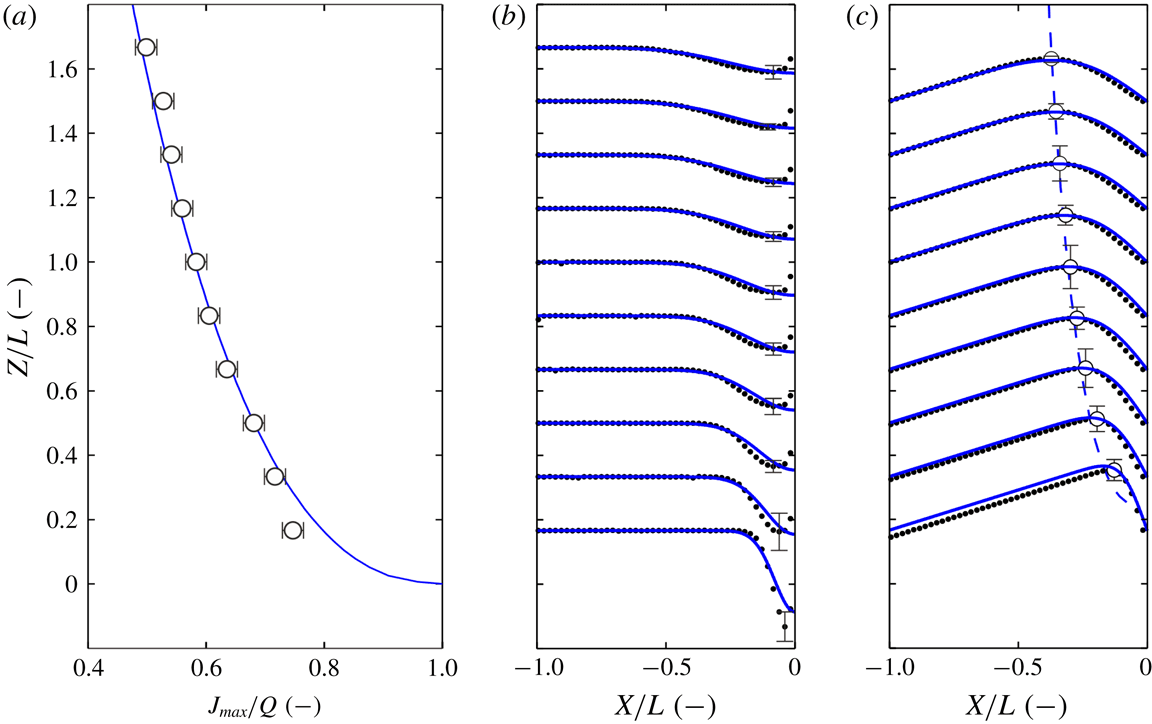
Results obtained via this calibration procedure are presented in figure 8 for one of the experimental runs. In figure 8(a), relation (4.5) is compared with the measured data for the
 $K$
value yielding the best fit. In figure 8(b), we then compare the theoretical profiles
 $W_{0}(X,Z)$
obtained with this
 $K$
value with the measured vertical velocity profiles. Finally, in figure 8(c), we compare the theoretical profiles
 $J(X,Z)$
with the corresponding experimental profiles. In addition to matching well the values of maximum current
 $J_{max}(Z)$
, on which the fitting was performed (figure 8
a), the results show good agreement for other features of the deep flow, including the detailed velocity profiles (figure 8
b) and the locus
 $X_{max}(Z)$
where the maximum current
 $J_{max}$
is attained (figure 8
c).
Comparison of the kinematic theory (blue curves) with experimental measurements (black symbols) for the deep flow region (run 2): (a) dependence of maximum horizontal current
 $J_{max}$
on elevation above orifice
 $Z$
, used to calibrate the diffusivity
 $K$
; (b) vertical velocity profiles
 $W(X,Z)$
; (c) horizontal current profiles
 $J(X,Z)$
, with locus of maximum values indicated by dashed line (theory) and circles (experiment). The error bars indicate
 $\pm$
one standard deviation, estimated from measurements of three repeat experiments for the same conditions, and multiplied for clarity by factors 20, 40 and 3 for panels (a), (b) and (c) respectively.

Considering that the diffusivity
 $K$
is the only parameter requiring calibration, agreement is good overall. Nevertheless, there are some significant differences between the predicted and measured velocity profiles. Most conspicuously (figure 8
b), the experiments feature a zone of low velocity near the side wall above the orifice, the thickness of which grows with height. This departure from our assumed condition of perfect slip may be partly due to the use of wood strips for the sides. The same behaviour, however, was also observed by Maiti et al. (Reference Maiti, Das and Das2016) in their experiments conducted in an eccentric silo made entirely from acrylic (polymethyl methacrylate) plates. Regardless of the side wall material, it is likely that grain mobility near the sides is reduced due to corner effects (grains in contact with both the front and side walls). This vertical boundary layer is not modelled by the theory, which instead assumes perfect slip along the side walls. Fortunately (figure 8
c), this local discrepancy exerts a limited influence on the integrated granular current profiles
 $J(X,Z)$
, hence its effect on the dynamics of the avalanching layer is expected to be small.
Variation of the dimensionless diffusivity with the dimensionless gap thickness for all experimental runs.

Using the larger set of experiments, in which we varied the outflow discharge, silo gap thickness and grain diameter (see table 1), we can further investigate the influence of these parameters on the calibrated diffusivity
 $K$
. The results, plotted in figure 9, are unexpectedly simple. For the range of conditions examined,
 $K$
is simply proportional to the gap thickness
 $B$
, satisfying to a close approximation the linear relation
 $K=\unicode[STIX]{x1D706}B$
, where
 $\unicode[STIX]{x1D706}=0.26$
. When the gap thickness is held constant,
 $K$
is independent of the discharge
 $Q$
, consistent with the rate-independent character of the kinematic model. Likewise,
 $K$
is found to be independent of the grain diameter
 $D$
.
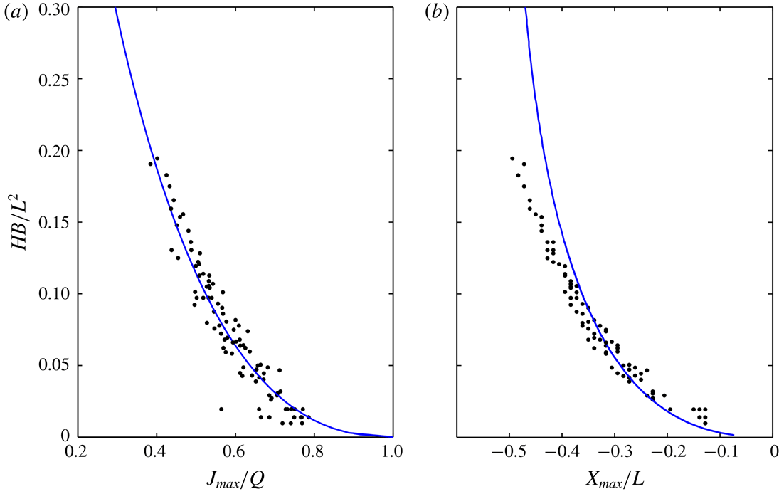
Comparison of the deep flow theory (blue line) with all experimental measurements (black dots): (a) maximum current
 $J_{max}$
; (b) location
 $X_{max}$
where the maximum current occurs.

As a consequence of this simple dependence, the
 $\hat{J}_{max}$
and
 $\hat{X}_{max}$
data for all the experimental runs should collapse together when plotted against dimensionless number
 ${\hat{H}}=HB/L^{2}$
. This is checked in figure 10. Upon substituting
 $\hat{Z}=\unicode[STIX]{x1D706}{\hat{H}}$
in (4.4), the data collapse and agree closely with the theoretical curve
 $\hat{J}_{max}({\hat{H}})$
(figure 10
a). Agreement for the locus
 $\hat{X}_{max}({\hat{H}})$
is also good (figure 10
b). The two-dimensional deep flow pattern above the orifice, therefore, is effectively the same for all cases when plotted in the dimensionless variables
 $(\hat{X},{\hat{H}})$
. To test whether this holds more generally, one would need to vary parameters over a broader range. For instance, it is unclear if the same reduction would hold for grains and walls of materials different from glass, which would affect their frictional properties. For the present experimental conditions, however, this reduction to a single dimensionless flow pattern accounts well for the deep flow observations.
4.2 Surface flow comparison
Once the basal forcing is known from the kinematic model, the dynamic model can be used to predict the surface avalanching flow. For this purpose, we estimate the basal normal velocity
 $\text{}\underline{w}_{0}$
or equivalently the basal streamfunction
 $\text{}\underline{\unicode[STIX]{x1D713}\!}_{\,0}$
from the analytical solutions (2.8) and (2.9). For the diffusivity, we adopt the values
 $K=\unicode[STIX]{x1D706}B$
estimated from the gap thickness
 $B$
using the linear relation calibrated in the previous section. For the rheological coefficients
 $\unicode[STIX]{x1D707}_{0}$
and
 $\unicode[STIX]{x1D712}$
, we adopt the values determined in § 3 from previous experiments by Jop et al. (Reference Jop, Forterre and Pouliquen2005) using the same granular material. Detailed comparisons will be presented for two runs, corresponding respectively to gap thicknesses
 $B=3.5$
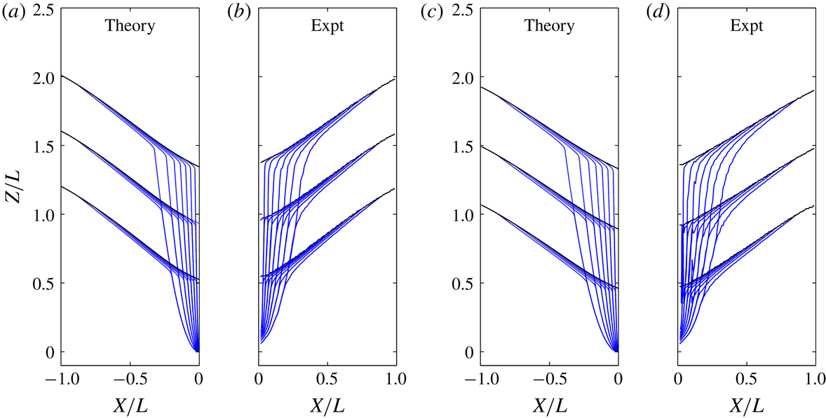
and 5 mm. In figure 11, we first compare predicted and measured streamfunctions for the entire flow field, at three successive times. The streamlines shown represent equally spaced streamfunction contours, hence the distance between contours is inversely proportional to the discharge through the corresponding streamtube. For the theory, the streamfunction is obtained from
 $$\begin{eqnarray}\unicode[STIX]{x1D6F9}=\unicode[STIX]{x1D6F9}_{0}+\unicode[STIX]{x1D713}-{\displaystyle\mathop{\unicode[STIX]{x1D713}}\limits_{{\sim}}},\end{eqnarray}$$
where the first term represents the deep flow, the second term surface avalanching and the third their common part that must be subtracted in order not to be counted twice. This approach is used in boundary layer problems to match inner and outer solutions (Kevorkian Reference Kevorkian1990). By analogy, the same approach can be used here to bridge between the avalanching and deep flow models. In our case, however, a more formal boundary layer analysis is not feasible because we do not know the more general equations that would reduce to the avalanching and deep flow models in the appropriate limits. For the experiments, the streamfunction is obtained from the measured velocity field
 $(U,W)(X,Z)$
by integrating
 $U$
column-wise from the bottom and
 $W$
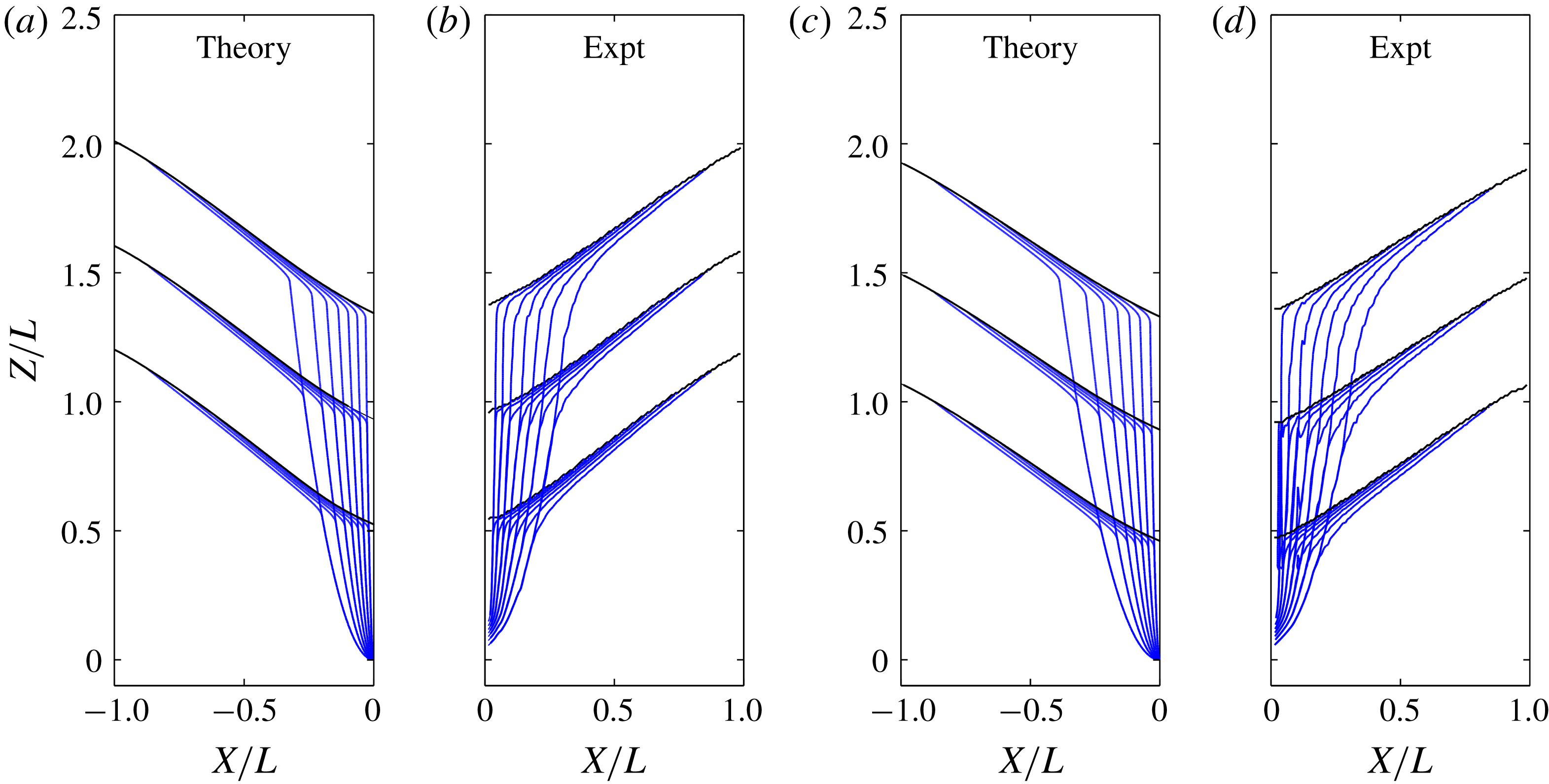
row-wise from the far side wall, then averaging the two results. Side by side comparisons between the theoretical and experimental streamlines obtained in this fashion are shown in figure 11. Going from top to bottom, the streamlines are first evenly spaced across the silo width, due the quasi-steady drawdown of the free surface. They then get focused by the avalanching layer, where the streamlines become very closely spaced, to connect with the uneven deep flow streamlines at their base. Thereafter, the streamlines gradually converge toward the orifice where they again become closely spaced. Theory and experiment are seen to be in good agreement regarding this overall pattern.
Comparison of predicted and measured streamlines for two different gap thicknesses, at three successive times: (a) prediction, and (b) measurements, for gap thickness
 $B=3.5~\text{mm}$
(run 3); (c) prediction, and (d) measurements for gap thickness
 $B=5~\text{mm}$
(run 5). Streamlines are plotted at equal streamfunction increments, each corresponding to
 $1/8$
of the total outflow discharge.
In figure 12, we compare predictions and measurements for the granular velocity fields. At five equally spaced times during the descent, we compare calculated results for the downslope velocity
 $u(x,z,t)$
(figure 12
a,c) with measured results for the magnitude of the velocity norm
 $((U-U_{0})^{2}+(W-W_{0})^{2})^{1/2}$
, from which the deep flow was subtracted (figure 12
b,d). On all panels, the last, lowermost snapshot shows the magnitude of the total velocity when the avalanching layer approaches the orifice level. In both theory and experiment, the avalanching layers exhibit lenticular depth profiles, with vanishing depths at both side walls and maximum depths
 $h_{max}$
that occur towards the orifice side of the silo. This asymmetry and the steepness of the avalanching layer become stronger as the surface descends closer to the orifice, becoming more strongly influenced by its localized pull. Surface velocities likewise accelerate as the avalanching layer drops.
Comparison of predicted and measured granular velocity fields for two different gap thicknesses, at six successive times: (a) prediction, and (b) measurements, for gap thickness
 $B=3.5~\text{mm}$
(run 3); (c) prediction, and (d) measurements for gap thickness
 $B=5~\text{mm}$
(run 5). Colours from blue to red indicate increasing velocity magnitude.

Comparison of the left and right panels of figure 12 further shows the influence of gap thickness
 $B$
on the avalanching flows. The maps of figure 12(a,b) correspond to gap thickness
 $B=3.5~\text{mm}$
, whereas those of figure 12(c,d) correspond to gap thickness
 $B=5~\text{mm}$
. For the larger gap thickness (figure 12
c,d), kinematic diffusion is stronger, hence a less localized surface drawdown by the deep flow. The maximum discharge
 $q_{max}$
that the avalanching layer must transfer to even out the drawdown is therefore reduced, hence weaker avalanching flows. The larger gap thickness, moreover, reduces the relative magnitude of wall friction, leading to deeper and slower avalanching layers for the same discharge. Note that this does not imply any change in the magnitude of the wall friction coefficient, assumed constant in the theory. For increasing gap width, the magnitude of the wall friction force relative to the other terms decreases because, in the width-averaged equation (2.13) and the ensuing depth-integrated equations, the wall friction force per unit width
 $-2\unicode[STIX]{x1D70F}_{W}/B$
is the only term that gets divided by the width
 $B$
. For the smaller gap thickness (figure 12
a,b), kinematic diffusion is weaker hence the deep flow drawdown is more concentrated above the orifice. The induced maximum avalanching discharge
 $q_{max}$
is therefore greater. Due to the smaller gap thickness, wall friction causes the avalanching layers to reduce their depth and steepen their inclination. As a result of these different effects, surface velocities are significantly increased compared to figure 12(c,d), even though the discharge
 $Q$
through the orifice is nearly the same.
Although the free surface is nearly linear for the wider gap (figure 12 c,d), for the thinner gap the surface curvature is more pronounced, transitioning from concave downward to concave upward going from upstream to downstream (figure 12 a,b). As it nears the orifice wall, the avalanching layer cusps upwards as it thins to a sharp tip. Similar behaviour was earlier described for symmetric silos, with avalanching layers that cusp upwards as they reach the silo axis of symmetry (Samadani et al. Reference Samadani, Mahadevan and Kudrolli2002). Although this behaviour was interpreted as resulting from shock formation, our shallow flow theory captures this phenomenon without a shock. Similar behaviour can be observed for flows in rotating drums, where the granular free surface goes from straight to curved as the rotation rate increases (Rajchenbach Reference Rajchenbach1990).
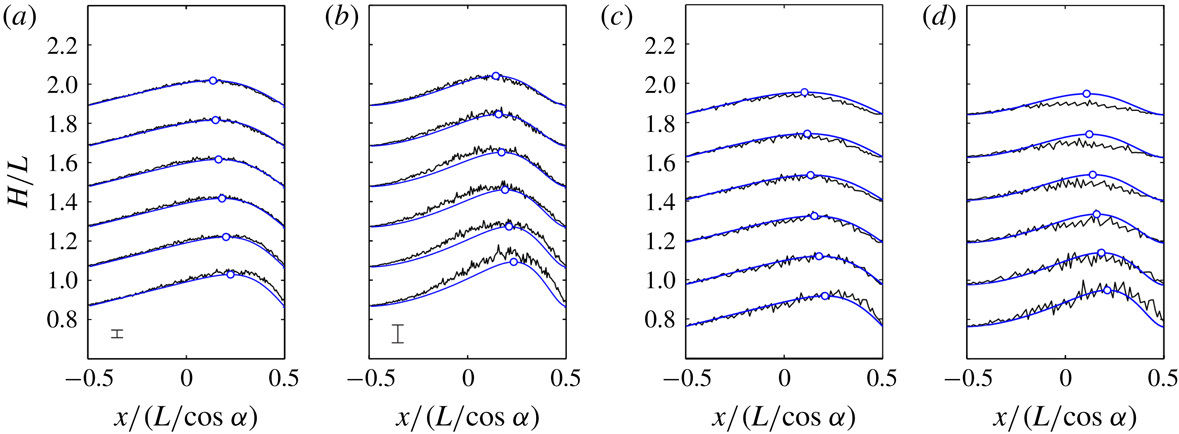
To make comparisons more precise, figure 13 plots together theoretical and experimental profiles for two depth-integrated quantities associated with the avalanching layers: the depth-integrated discharge
 $q=\int \,u\,\text{d}z$
, and the depth-integrated kinetic energy,
 $k=\int (u^{2}\,\text{d}z)/2$
, both varying with height above orifice
 $H$
and with the downslope coordinate
 $x$
. Since the discharge profile is controlled by the deep flow, the comparisons for
 $q$
represent a test of the kinematic model (figure 13
a,c). For a given discharge profile, on the other hand, the kinetic energy profile is controlled by the avalanche dynamics, hence comparisons for
 $k$
represent a test of the dynamic model (figure 13
b,d). In both the theory and experiments, peaks in
 $q$
and
 $k$
occur further downstream as the granular surface drops and approaches the orifice. Also, profiles for the smaller gap thickness (figure 13
a,b) are more asymmetric than profiles for the larger gap thickness (figure 13
c,d). Finally, the profiles for
 $k$
are more strongly peaked than the profiles for
 $q$
. For all these features, fairly good agreement is registered between theory and experiment. Although the measured signal for the kinetic energy is noisier, the level of agreement obtained for
 $q$
and
 $k$
indicates that both the kinematic and dynamic models perform reasonably well.
Comparison of theory (blue lines) and experiment (black lines) for profiles of discharge and kinetic energy, at six successive times during the descent of the avalanching layers, for two different gap thicknesses: (a) discharge profiles
 $q(x)$
, and (b) kinetic energy profiles
 $k(x)$
, for gap thickness
 $B=3.5~\text{mm}$
(run 3); (c) discharge profiles
 $q(x)$
, and (d) kinetic energy profiles
 $k(x)$
, for gap thickness
 $B=5~\text{mm}$
(run 5). Circles indicate peaks in the predicted profiles. The error bars in (a,b) indicate
 $\pm$
one standard deviation, estimated from three repeat experiments for the same conditions.

5 Conclusion
In the present work, theory and experiment were used to investigate granular surface avalanching in narrow silos. Provided that the deep and shallow flows exhibit a clear separation of scales, it was shown that narrow silo avalanching can be described well by combining kinematic and dynamic models, matched along an approximate basal interface. The resulting theory captures both the rate-independent character of the deep flow and the rate-dependent behaviour of the avalanching layer, each in the frame of reference where they can be considered steady. For the deep flow, the measured velocities and the induced forcing at the base of the avalanching layer are described fairly well by the kinematic model, subject to a linear relation between the kinematic diffusivity and the silo gap thickness. For the surface flow, on the other hand, the shape of the avalanching layer and longitudinal profile of depth-integrated kinetic energy are well predicted by the dynamic model. Combined together, the two models also produce velocity fields and streamlines that agree fairly well with experiments over the entire domain.
More general continuum formulations have been proposed (Staron et al. Reference Staron, Lagrée and Popinet2014; Dunatunga & Kamrin Reference Dunatunga and Kamrin2015; Lee, Huang & Chiew Reference Lee, Huang and Chiew2015; Daviet & Bertails-Descoubes Reference Daviet and Bertails-Descoubes2016), and may be able to model subsidence-driven granular avalanching under less restrictive assumptions. Nevertheless, the simple approach proposed in the present work presents various advantages. First, it applies to precisely the conditions likely to tax the capabilities of modelling approaches like discrete element simulations or Navier–Stokes solvers. The number of grains contained in the present experimental silos, for instance, would require very large computational resources to be modelled by discrete particles. Resolving the steep gradients and large convective inertia of the present avalanching layers, likewise, would require very small mesh cells and small time steps for Navier–Stokes-type computations. Another advantage of our semi-analytical approach is to clarify the physical role played by different parameters.
Nevertheless, the approach of the present paper is currently subject to various limitations. In particular, it is restricted to two-dimensional, quasi-steady flows of mono-disperse grains over deep erodible beds of the same composition, assumed governed by wall friction and by the linearized
 $\unicode[STIX]{x1D707}(I)$
rheology. Further research will be needed to overcome these limitations and possibly address other applications like flows partly controlled by non-erodible beds (Parez et al.
Reference Parez, Aharonov and Toussaint2016; Fernández-Nieto et al.
Reference Fernández-Nieto, Garres-Díaz, Mangeney and Narbona-Reina2018; Sarno et al.
Reference Sarno, Carleo, Papa and Villani2018), and unsteady non-uniform flows like granular column collapse (Chou et al.
Reference Chou, Lee, Chung and Hsiau2012; Ionescu et al.
Reference Ionescu, Mangeney, Bouchut and Roche2015; Lee et al.
Reference Lee, Huang and Chiew2015).
Acknowledgements
A post-doctoral stay by C.-Y.H. and a sabbatical visit by H.C. at IUSTI, Aix-Marseille Univ., provided the opportunity for the present research. In Marseille, the hospitality of O. Pouliquen and E. Guazzelli is gratefully acknowledged. We also thank Y. Forterre for providing materials and advice. Some of the theoretical ideas were earlier explored with C. Stark. This work was undertaken under the auspices of the Labex MEC (ANR-10-LABX-0092) and of the A*MIDEX project (ANR-11-IDEX-0001-02), funded by the Investissements d’Avenir program managed by the French National Research Agency (ANR). Additional financial support was provided by the Ministry of Science and Technology, Taiwan, and the program for research excellence of National Taiwan University.