




No CrossRef data available.
Article contents
- Abstract
- REFRAMING INQUIRY INTO VOTER TURNOUT
- AGING, INERTIA AND THE TWO HABITS OF VOTING
- A DEVELOPMENTAL THEORY OF TURNOUT
- THE LIMITATIONS OF CROSS-SECTIONAL AND COHORT METHODS
- THE LATENT GROWTH CURVE MODEL
- DESCRIPTION OF DATA AND SEQUENCE OF MODEL ESTIMATION
- RESULTS I: PARENTAL INFLUENCE ON INITIAL TURNOUT AND GROWTH
- RESULTS II: HIGH SCHOOL INFLUENCES ON TURNOUT
- RESULTS III: LIFE EVENTS BETWEEN 1965 AND 1968
- RESULTS IV: LIFE EVENTS AFTER 1968
- SUMMARY AND IMPLICATIONS
- References
Becoming a Habitual Voter: Inertia, Resources, and Growth in Young Adulthood
Published online by Cambridge University Press: 03 March 2004
Article contents
- Abstract
- REFRAMING INQUIRY INTO VOTER TURNOUT
- AGING, INERTIA AND THE TWO HABITS OF VOTING
- A DEVELOPMENTAL THEORY OF TURNOUT
- THE LIMITATIONS OF CROSS-SECTIONAL AND COHORT METHODS
- THE LATENT GROWTH CURVE MODEL
- DESCRIPTION OF DATA AND SEQUENCE OF MODEL ESTIMATION
- RESULTS I: PARENTAL INFLUENCE ON INITIAL TURNOUT AND GROWTH
- RESULTS II: HIGH SCHOOL INFLUENCES ON TURNOUT
- RESULTS III: LIFE EVENTS BETWEEN 1965 AND 1968
- RESULTS IV: LIFE EVENTS AFTER 1968
- SUMMARY AND IMPLICATIONS
- References
Abstract
This paper reframes our inquiry into voter turnout by making aging the lens through which the traditional resource and cost measures of previous turnout research are viewed, thereby making three related contributions. (1) I offer a developmental theory of turnout. This framework follows from the observation that most citizens are habitual voters or habitual nonvoters (they display inertia). Most young citizens start their political lives as habitual nonvoters but they vary in how long it takes to develop into habitual voters. With this transition at the core of the framework, previous findings concerning costs and resources can easily be integrated into developmental theory. (2) I make a methodological contribution by applying latent growth curve models to panel data. (3) Finally, the empirical analyses provide the developmental theory with strong support and also provide a better understanding of the roles of aging, parenthood, partisanship, and geographic mobility.
Information
- Type
- Research Article
- Information
- Copyright
- © 2002 by the American Political Science Association
Every presidential election raises questions about voter turnout in the United States and, in particular, the very low turnout of young voters. Why is voter turnout so much lower among the youngest citizens? Can interventions addressed specifically toward young voters likely to have a lasting impact? Are some groups of young citizens especially cut off from the political system, and could this have consequences for their participation later in life?
How can we generate better answers to questions such as these? I argue that we need to reframe our approach to voter turnout by subsuming the familiar costs–resources framework within a developmental perspective. Doing so leads to more precise and qualified questions and spurs use of more appropriate models. I show that doing so can yield more valid and satisfying answers to questions about voting behavior.
REFRAMING INQUIRY INTO VOTER TURNOUT
Turning out to vote is the most common and important act citizens take in a democracy and, therefore, is one of the most important behaviors for scholars of democratic politics to understand. And yet, it is not well understood. (Aldrich 1993, 246)
Scholars have also examined factors that increase the costs of voting. Geographic mobility, for example, can substantially increase the barriers to voter registration (Squire, Wolfinger, and Glass 1987). Others have explored the disruptive effects of severe hardship (Rosenstone 1982) and the exhaustion and time demands associated with raising young children (Plutzer 1998).
The twin foci of resources and costs have yielded a large number of research findings but not a good sense of how the many factors fit together or when and where variables will matter most. That is, the many findings do not yield a set of conditions and qualifications that marks a mature theory.
The many variables associated with turnout make much more sense when viewed through the lens of aging and the development of the habit of voting. Consistent with this idea, I offer a developmental framework for understanding turnout. Highlighted in this framework are the notions of starting level (the probability that citizens vote in their first eligible election) and inertia (the propensity for citizens to settle into habits of voting or nonvoting). The developmental framework distinguishes among factors influencing the starting level, factors that can shift a voter from one inertial state to another, and factors that interrupt established habits. Methodologically, the developmental perspective lays bare many questionable assumptions and practices characterizing almost all previous research on life-cycle and life-experience explanations for turnout. To address these problems I apply latent growth curve models and explain their applicability to developmental processes more generally. I go on to test key assumptions of the developmental theory and to reassess conclusions drawn from cross-sectional analyses.
AGING, INERTIA AND THE TWO HABITS OF VOTING
The distinctive relationship between age and voter turnout has intrigued students of electoral behavior since at least the early 1960s. Milbrath (1965, 134) cites eight early reports of steep rise in turnout in young adulthood followed by gradual increases until voters reach their sixties. Verba and Nie (1972) proposed a number of “life-cycle” explanations; this in turn spurred many others to consider how and why this rise-and-fall pattern occurs in virtually every survey of U.S. electoral behavior (e.g., Jennings and Markus 1988; Strate et al. 1989; Miller and Shanks 1996; Highton and Wolfinger 2001).
In fact, the effect of age is comparable to the strong effect of education. The 1998 Current Population Survey, for example, shows a 40-point turnout gap between those who completed less than ninth grade (24% turnout) and those with an advanced degree (64%). But the gap between those 18–24 years old and those older than 65 is 46 points (17 compared to 63%). More important, aging may come to the fore because as citizens get older, experience can compensate for low levels of education (Wolfinger and Rosenstone 1980, 60).
Nevertheless, scholars in the resource and SES tradition rarely pay much attention to age (exceptions include Strate et al. 1989; Jankowski 2001). Indeed, they sometimes leave the effect of age unreported along with those of other “control” variables.1
See, e.g., many tables of Verba, Schlozman, and Brady (1995, chaps. 12, 15). To be fair, the authors of Voice and Inequality acknowledge that “there is more to the impact of age than the analysis in this chapter can reveal—but that must wait for future research” (p. 423).
Voting as a “Habit” and Path Dependence
Virtually all major works on turnout have concluded that voting behavior is, in part, a gradually acquired habit. Milbrath explicitly invokes psychological concepts of reinforcement and “habit strength” to characterize habitual voting (1965, 31; see also Verba and Nie 1972, 148; Miller and Shanks 1996, 17, 62). In short, although the terminology varies, there is a longstanding agreement that voting behavior is habitual. Thus, it is useful to think about civic development as a largely path-dependent process.
The process begins as young citizens confront their very first election. Each has a latent probability of voting resulting from parental, demographic, and personal factors. Some will vote and become habitual voters, but most will not and are likely to remain nonvoters in subsequent elections. That is, most new citizens show evidence of inertia. Inertia is rather different from persistence, a central organizing concept in political socialization research (Sears 1990; Searing, Schwartz, and Lind 1973). The notion of persistence suggests that one can find the origins of adult attitudes and ideology in events and influences that occurred many years earlier. In contrast, inertia suggests that the roots of current turnout can be found in voting behavior in the previous one or two elections.
Almost all habitual nonvoters gradually increase their probability of voting and eventually make the transition to being habitual voters. Some do so almost immediately, but others remain habitual nonvoters for many elections. From this perspective, the key explanatory task is identifying the factors that influence how quickly different voters make the transition from one inertial state to another. Of course, habitual voters are sometimes thwarted from voting in a particular election. But failing to vote once does not shift them back to nonvoting. In most cases, the disruption is short-term and they return to their habitual behavior. Once voters are on the path of regular voting, factors that were once important (parental influences, educational attainment) diminish.
A DEVELOPMENTAL THEORY OF TURNOUT
This simple framework allows a new and useful integration of prior research, as I now attempt to demonstrate.
Starting Levels of Turnout
As young citizens confront their first election, all of the costs of voting are magnified: they have never gone through the process of registration, may not know the location of their polling place, and may not have yet developed an understanding of party differences and key issues. Moreover, their peer group consists almost entirely of other nonvoters: their friends cannot assure them that voting has been easy, enjoyable, or satisfying.
Young people also lack many of the resources that can promote participation. Because they have little disposable income, they are not attractive targets for parties seeking campaign contributions or for interest groups mounting direct mail campaigns. Few of them own homes, have stakes in community politics, or have completed college. Thus it is not surprising that few young citizens are registered to vote (Timpone 1998) and their turnout is relatively low.
Nevertheless, many young citizens do vote—presumably because “the start-up costs of voting are not borne equally by all young people” (Wolfinger and Rosenstone 1980, 60). A few have resources that allow them to overcome the high costs of first-time registration and first-time voting. These resources can come from their parents or from their own achievements. Verba, Schlozman, and Brady (1995, chap. 15) distinguish between parental socioeconomic status and parental political involvement. Parental education promotes offspring education and offspring political knowledge, including such mundane information as how to register and where to vote. Thus political knowledge is an asset that can directly offset costs of initial turnout. Parental political involvement can provide both behavior to model and campaign-relevant information that children rarely get from formal schooling.
Parental resources combine with young citizens' own achievements before their first election. Although they may not have yet completed their formal education, they may have acquired some political knowledge and may have developed an interest in public affairs (reflected, e.g., in reading newspapers or weekly news magazines). They may also have some partisan attachments, though these are likely to be malleable over the long term and may therefore have weak or transient effects (Jennings and Niemi 1981).
In sum, a variety of factors—all previously identified by other authors—should be expected to influence starting levels of turnout. However, it is unclear whether any of these factors will matter in the future or whether their effects will dissipate because of the inertia that typically follows.
The Nature of Inertia and the Habits of Turnout
A citizen's voting history is a powerful predictor of future behavior. This is easily illustrated by using self-reports of turnout from those who completed the 1972–1976 National Election Studies (NES) panel study (Center for Political Studies 2000). Of the 516 respondents who reported voting in both 1968 and 1972, only 3% missed voting in both the 1974 and the 1976 elections. In contrast, of the 57 respondents who reported missing two consecutive elections (either 1968–72 or 1972–74), more than two-thirds did not vote in the next election.
Unfortunately, the nature of inertia is undertheorized. Here, I offer some speculations, the specifics of which will remain for future research to fill in. First, the two inertial states are very different. The stability of habitual nonvoting is one that most citizens “outgrow” and is, therefore, weaker. Citizens can outgrow the nonvoting habit if the costs of voting remain relatively constant over the life course but the resources available to overcome those costs increase. Income, for example, tends to increase in young adulthood, and this may gradually increase the likelihood of being recruited into electoral politics (Verba, Schlozman, and Brady 1995, chap. 5). Second, cognitive resources—especially political knowledge—should increase with age (Wolfinger and Rosenstone 1980; Strate et al. 1989; delli Carpini and Keeter 1996). Third, life events such as marriage, home ownership, and having children in school often increase community ties, enhance the relevance of local elections, and increase the perceived stakes of electoral outcomes (Verba and Nie 1972). Fourth, even constant activities can have cumulative impacts. For example, young voters who attend weekly religious services may gradually acquire politically relevant resources [information from politicized sermons, opportunities for leadership and public speaking, etc. (see Verba, Schlozman, and Brady 1995)].
Overall, many resource (e.g., socioeconomic status, cognitive assets, political engagement, social networks) and life-cycle variables (e.g., marriage, home ownership) act on habitual nonvoters by increasing their probability of voting in subsequent elections. Each resource variable should be expected to speed the transition from nonvoter to habitual voter.
The Inertia of Habitual Voters and Temporary Disruptions
Both habitual nonvoters and habitual voters display inertia, but the nature of that inertia differs. Nonvoters must overcome bureaucratic barriers (most notably registration) and costs of various types (e.g., information costs). These same factors, however, contribute to stability once a citizen has crossed the threshold and voted once. Although residential mobility is common, most voters do not move in a four-year period. So once they register and vote, the barrier of registration is unlikely to come into play in the next election or two. Similarly, once voters attain a certain degree of political knowledge—for example, finally understanding some key differences between the parties—they are unlikely to forget it or find that their knowledge has become obsolete in the next few elections.
Norms also contribute to inertia. Voting for the first time is likely to bring positive reenforcement from friends, family, and co-workers. As voters age, their peer cohort has increasingly higher participation rates and they eventually move out of age-homogeneous settings (e.g., college residences) and into others (workplaces, community organizations) where the average levels of political knowledge and turnout are higher. Thus, as young citizens take on more adult roles, they are likely to be subject to more and more intense participation norms.
For all of these reasons, after young citizens vote once, they should only occasionally experience an increase in the costs of voting relative to their resources and social pressures. A reversal may occur as a result of a major life event that creates immediate demands for one's time and attention. For example unemployment has a noticeable effect on voter turnout but only if the onset of unemployment was very close to the election; if more than a few months pass, voters seem to rebound (Rosenstone 1982). This pattern of a “rebound” raises the question, “Rebound to what?”
A rebound implies that severe economic dislocations will show up as major factors discouraging habitual voters, but severe disruptions may be largely irrelevant to nonvoters because most would not vote anyway. At most, hardships are just one of many barriers facing habitual nonvoters or newly eligible citizens. Therefore, smaller hardship effects should be evident among the very young because so few are habitual voters.
The central disruption factor that has been studied to date is residential mobility (Squire, Wolfinger, and Glass 1987). Habitual voters who move from one precinct to another usually must reregister to vote and discover the location of a new polling place. Thus, residential mobility may temporarily disrupt their regular pattern. Like other disruptive factors, residential mobility is primarily a factor affecting habitual voters, and its effects should be considerably less evident among younger citizens than their older counterparts.
To summarize, voter turnout is developmental and characterized by modest inertia for nonvoters and strong inertia for voters. Key explanatory variables from previous research can be characterized in terms of whether they affect starting levels or the speed of transition or whether they function primarily to disrupt established patterns. This relatively simple framework provides the basis for more precise hypotheses (e.g., that the effects of parental characteristics dissipate rather than persist and that disruptions such as mobility and parenthood are likely to have increasing explanatory power as citizens age).
Before moving putting these expectations to the test, it is useful to examine the methodological challenges involved in analyzing turnout via cross-sectional survey data and to introduce an analytic approach that has not previously been exploited in research on turnout.
THE LIMITATIONS OF CROSS-SECTIONAL AND COHORT METHODS
Several scholars have focused specifically on understanding life-cycle effects. Yet previous efforts are characterized by data and models that do not correspond to each other. Using cross-sectional data to make inferences about the life-cycle or the life-experience process is risky for several reasons. First, it is extremely difficult to avoid the “fallacy of assumed reversibility.” Lieberson (1985) observes that we tend to interpret a regression slope of +1 as meaning both that “a one unit increase in X is associated with a one unit increase in Y” and that “a one unit decrease in X is associated with a one unit decrease in Y.” If the developmental theory is essentially correct in its core assertion of inertia, this may be theoretically implausible. For example, consider two individuals whose earnings at age 30 place them in the 99th percentile. Based on current research, each is expected to have higher than average political participation. Suppose that four years later, one's earnings plummet to the median. If voting is an acquired habit, it makes no sense to predict that her participation will fall to average levels. Nevertheless, this is exactly what most cross-sectional models force the researcher to assume. The degree of misspecification is directly proportional to the extent to which certain life events produce gains in participation that are more difficult to reverse than they were to acquire. This developmental asymmetry can be modeled cross sectionally if different variables are used to distinguish income gains from income losses (e.g., Plutzer and Wiefek 1998). However, a developmental statistical model provides a much better fit between theory and method.
A second problem is endogeneity. If voting is an acquired habit, then the proximate causes of voting in election t are largely contained in the information represented by the turnout variable for election t − 1, which in turn is largely determined by turnout in prior elections. The older the respondent, the longer the causal chain. If voting in the current election is an indicator of one's long-term probability of voting, then many “independent variables,” such as income and marital status, are endogenous to the latent variable that cross-sectional turnout actually measures. Cross-sectional studies could deal with this if turnout could be decomposed into a latent long-term probability and a short-term response to recent personal, macroeconomic, and political conditions. Yet this could be accomplished only with reliable and valid turnout histories for each respondent. Thus, the potential problems of irreversibility and ambiguous causal order in cross-sectional models make a developmental analysis preferable.
A third limitation in most cross-sectional studies is the confounding of age with generation. Even in the most careful analyses (e.g., Strate et al. 1989) it is never clear whether age is helping to explain life-cycle, life-experience, or generational effects.
Cohort analysis has complementary problems (e.g., Miller and Shanks 1996, chap. 4): they do not permit inferences about individual behavior and rarely contain enough cases to enable subgroup analysis. Moreover, subgroups based on changeable statuses (e.g., married, employed, childless, Southern, or home owner) cannot be studied at all (Riley 1973; see also Converse 1976). In short, cohort analysis cannot support reliable inferences concerning the effects of individual experiences that lie at the heart of the life- cycle and life-experience perspectives.
THE LATENT GROWTH CURVE MODEL
A superior approach, when appropriate data are available, is provided by latent growth models. To build such a model, one first theorizes about a single individual who is first eligible to vote in election t and continues to be eligible to vote in subsequent elections, t + 1, t + 2, etc. At each election the citizen is observed to vote or not and this is conceived as an indicator of a latent probability of turnout. This can be modeled as
where Y is a dummy variable denoting whether the individual voted in election t, ELECTION is a variable coded 0, 1, 2,…T1 − 1, and T1 is the number of elections observed for each individual. Two parameters describe an individual's latent growth curve, with β0 corresponding to the height of the curve as it crosses the y axis and β1 the steepness of the increase or decrease. Each respondent's first eligible election is coded as ELECTION = 0, so that the intercept, β0, indicates the individual's starting level and the slope, β1, estimates the growth in the latent probability of voting—hence, the characterization of a “latent growth curve.” This model can be estimated by logistic (or probit) regression. If the number of elections is three or more, the model will have a residual, which is designated r here. Therefore, the model for each individual is
A sample of N individuals is thus conceived of varying among themselves in two ways. First, citizens have varying probabilities of voting in their first eligible election, leading to N different values of β0. Second, each has a unique developmental trajectory, leading to N different values of β1. Thus, in a sample, the parameters for the ith individual, β0i and β1i, are conceived as random variables. In all past studies, these two components of turnout have been combined in cross-sectional turnout and predicted by the same set of variables. This failure to separate out starting level from growth (or decline) has both methodological and theoretical consequences. Methodologically, it means that part of turnout is exogenous to many independent variables (the starting level for most individuals is determined before most predictor variables are observed), reversing the usual assumptions of causal inference.
The developmental theory implies that variables determined before an individual reaches voting age, such as parent's education, will have a greater impact on the starting point than on subsequent growth. Most other factors will affect growth rates. This distinction is reflected in two equations that capture the effects of various independent variables on β0 and β1, respectively. The first equation predicts one's likelihood of voting in one's first eligible election:
where β0i is the intercept term from Eq. (2) (in units of logged odds), γ00 is an intercept term, Z is a variable that affects initial turnout and (potentially) long-term growth, γ01 is the effect of Z on initial turnout, and u0i is the unexplained variance in person i's starting level. And the second model predicts each individual's rate of growth over time:
where β1i is the slope parameter from Eq. (2), γ10 is an intercept term, Z is a predictor of the rate of turnout growth that occurs before t = 0, γ11 is the effect of Z on the rate of turnout growth, X is a predictor of the rate of turnout growth that occurs after t = 0, γ12 is the effect of X on the rate of turnout growth, and u1i is the unexplained variance in person i's growth rate.
Equations (3) and (4) comprise the essential model (sometimes called a hierarchical linear model; HLM), but they cannot be estimated separately. By substituting for β0 and β1, and subscripting for the ith person, Eq. (2) can be written
Rearranging terms gives
This model cannot be estimated by OLS or traditional methods of maximum likelihood because of the multiplicative term between the disturbance from Eq. (4) (u1i) and ELECTION, because of the correlation between the two disturbance terms (u1i and u0i), and because of the need to estimate the variance of the disturbances prior to estimation of the slopes and their standard errors. However, several reliable solutions are available. These use a doubly iterative procedure in which MLE iterations are augmented by empirical Bayes estimates. The models reported here were estimated by MIXOR 2.0 (Hedeker and Gibbons 1996).2
Bryk and Raudenbush (1992) provide a thorough introduction containing detailed references for those interested in the evolution of estimation solutions. For a more detailed discussion of estimation issues unique to problems with binary dependent variables, see Hedeker and Gibbons (1994, 1996), who also provide helpful references to the technical statistical literature.
DESCRIPTION OF DATA AND SEQUENCE OF MODEL ESTIMATION
I employ data from Jennings and Niemi's three-wave Student–Parent Socialization Study (Jennings 1972; Jennings and Niemi 1991; Jennings, Markus, and Niemi 1991; remerged in order to include respondents who did not complete the panel). High school seniors and one or both of their parents were interviewed in 1965, 1973, and 1982. The 1973 interview included questions concerning turnout in the 1968 and 1972 elections and the 1982 survey asked about voting in 1976 and 1980, providing self-reported turnout in four consecutive presidential elections. Analysis is restricted to students who were 21 years old on or before election day in 1968. The 1968 election is coded as election 0, with 1972, 1976, and 1980 coded as 1, 2, and 3, respectively. A summary of the marginal distributions of turnout in each election and a detailed description of how I treated missing data is provided in the Appendix.3
Timpone (1998) shows that a model's failure to distinguish between registration and turnout among the registered can lead to misleading interpretations. Unfortunately, the data include registration questions only for two of the four elections examined here, making it impossible to estimate a separate registration model or a two-stage selection model. However, it seems appropriate to assume that starting level is determined largely by the motivation to register and the resources to overcome registration hurdles. As citizens get older, registration becomes a smaller component of nonvoting.
Independent variables are in four blocks that lie at different points in a funnel of causality. These blocks correspond to the intergenerational transmission model of Verba, Schlozman, and Brady (1995, chap. 15). This framework presumes that the effects of early events are partially mediated by later ones, and this suggests using a block recursive strategy in which the total effects of variables early in causal chain are compared to their net effects after the addition of variables from later blocks [see Miller and Shanks (1996) for a similar approach]. Next I provide a summary of the independent variables.4
Documentation of the exact question wording of all variables descriptions of how items were combined into composite measures of various kinds is available from the author upon request.
Block I. Demographic and Parental Characteristics
Block I variables include sex, race, and three indicators of parents' socioeconomic status: educational attainment, reported family income, and the Duncan Occupational Prestige score for the head of household.
Five additional variables measure the political environment created by the parents. The first is a standard question about the parents' interest in politics; the second is the parents' score on a political knowledge quiz consisting of six factual items. Additional measures are scores on a three-item scale of political trust, parents' strength of party identification, and parents' self-reported vote in the 1964 presidential election.5
The maximum amount of information was extracted from the parent interview data. The mother was interviewed in one-third of the cases, the father in one-third, and both parents in one-third. In cases where both parents gave valid answers to questions about politics the answers were averaged.
Unless otherwise noted, all predictors that are numeric scales (e.g., family income and years of education) or have arbitrary metrics (attitude measures with agreedisagree responses) are standardized (mean of 0 and standard deviation of one), while dummy variables remain in their natural metric. This coding ensures that all predictors have a meaningful value of 0, aiding in interpretation of the intercept.
Block II. Youth Characteristics at the Completion of High School
This block includes resource measures based on interviews three years before the seniors became eligible to vote. I use self-reported high school GPA as an indicator of educational achievement. An index of activity in student politics and student organizations addresses activities whose recall was found to be important by Verba, Schlozman, and Brady (1995, chap. 14); here they are measured as a scale composed of indicators of having run for student office and of a holding leadership role in any student organization. A measure of church attendance serves as an indicator of community-based resources.
Three variables tap into psychological resources and political engagement. The first is a three-item engagement in politics scale, which is a standardized composite of expressed interest in politics and the frequency of both newspaper and newsmagazine readership.6
Factor analysis yields loadings that range from 0.69 (magazine readership) to 0.79 (newspapers) for the three items with an estimated reliability (Cronbach's α) of 0.61.
Block III. Events and Achievements Between High School and the First Election
Although the youth were not interviewed between 1965 and the 1968 election, the 1973 interview was sufficiently detailed to enable construction of measures for four key life transitions during this period. Two are potential resources and two are presumed disruptions. Dummy variables indicate whether each young adult had attended college (63% of the sample did so), was married in 1968 (28%), or became a parent before the 1968 election (15%).
A simple measure of geographic mobility was impossible to construct because the questionnaire did not ask when each move between 1965 and 1973 occurred. However, respondents indicated if and when they moved to another state, permitting the computation of a dummy variable indicating if a respondent moved across state lines between 1965 and 1968.
Block IV. Life Events and Achievements After the First Election
The last causal block includes a wide array of resources and disruptive factors. The resources include both events/achievements (reports of final educational level, economic status, marriage, parenthood, and community ties) and psychological/subjective measures (political engagement and political knowledge).
The reports of events and behaviors include most of the usual variables suggested in life-cycle research. All are measured as of 1973—less than a year after the 1972 election and prior to subsequent elections in 1976 and 1980. Thus, they capture events during the first five years of voting eligibility for each respondent. Three variables tap various aspects of socioeconomic status. An ordinal measure of “final” educational achievement is coded −1 for those who did not attend college, 0 for those with some college attendance, and +1 for those who completed a college degree. Family income is measured by an 18-category variable that has been standardized. Income differences tend to widen with age and may be a poor indicator of one's position in the stratification system at age 25. At that age, young attorneys and management trainees earn less than many skilled blue-collar workers even though the former understand that they are on a track toward an upper middle-class standard of living. I therefore include a dummy variable denoting whether the head of household has a professional, technical, or high managerial position.
Three variables tap aspects of community involvement and social ties: a dummy variable indicating home ownership, a four-category measure of frequency of church attendance (also standardized), and marital status (measured by two dummy variables indicating whether the respondent was married or divorced; never married is the omitted category). Divorce can be thought of as a disruption that can lower turnout.
Additional disruption measures include the number of residential changes since 1965 (standardized) and parenthood, as measured by two dummy variables. The first indicates the presence of school-age children (age six or older), and the second is coded 1 if the respondent has one or more children under six (but none older). Childless respondents are the omitted category.
Limitations of the Data
The Jennings and Niemi study constitutes the best (perhaps the only) data set that will permit estimating latent growth models of turnout. However, certain features of the data set bear on generalizibility. Most obviously, the period between 1965 and 1973 encompasses the escalation of the Civil Rights, antiwar, and campus free speech movements, along with related movements and political events. Undoubtedly, some of the parameter estimates would differ if a different cohort of high school seniors were studied (although it is difficult to anticipate which these might be).
Second, the study's design eliminates those who dropped out of high school prior to their senior year. In 1965 this was roughly 27% of the cohort. Thus, the restricted range of education almost surely narrows the range of several variables including parent education and SES, parent and student turnout, and youth's 1973 income. These probably have the effect of attenuating some relationships, yielding fairly conservative hypothesis tests and downwardly biased slopes (and relatively high percentages of self-reported turnout). The restriction in range almost surely exaggerates the speed with which high-resource and low-resource segments of the population converge in their turnout rates as they age.
Finally, with only four elections observed for each respondent, the smooth curves suggested by latent growth curve models represent a simplification. With a longer series of observations, life events producing dramatic short-term increases or temporary disruptions could be modeled more precisely (indicators of shocks preceding particular elections could be added to equation two). In the analyses summarized below, shocks will be reflected in substantial changes in the steepness of estimated growth curves, but these curves will nevertheless be estimated as smooth, monotonic functions.
Issues of Model Specification
Previous research suggests that all variables in Blocks I, II, and III are plausible predictors of turnout in the 1968 election. However, if these contribute to each individual's underlying probability of turnout in their first eligible election, it is not clear whether they should be expected to have additional impact on the rate of increase. Consider, for example, the impact of having parents with high levels of education, income, and political involvement. On the one hand, a rich cognitive environment could have a lasting legacy that provides an additional impetus toward political interest and participation, reflecting the idea that education provides the basis for further learning throughout the life course. Thus, a cognitively rich and politically engaged parental environment in childhood and adolescence might result in an acceleration turnout growth, reflected in a hypothesized positive effect on β1. Such a growth hypothesis will be tested for each predictor.
However, the effect of parental resources could diminish over time as the young citizen leaves home and is exposed to more recent effects of community transitions, socioeconomic achievements, and family formation. Thus, in the absence of strong theory or previous research, hypotheses of no effect on growth are at least as plausible as hypotheses of positive effects. Thus, the question of whether the β1 side of the model is over-specified cannot be resolved on theoretical grounds.
The initial model, therefore, will start with all Block I variables modeled as predictors of β0 and of β1. My standing expectation, however, is that all effects on β1 will be 0. For reasons of parsimony and to avoid potential problems of multicollinearity, insignificant predictors of β1 will not be retained when models add additional variables further along in the causal chain. This strategy strikes a balance between concerns about collinearity and the weak theoretical bases for hypotheses concerning long-term growth.7
I also estimated a saturated model containing all possible main effects and interactions for variables in all four blocks. Comparing these results with those in Table 7 reveals no sign changes and only two changes in statistical significance; the saturated model is not reported because of space constraints but the results are available from the author upon request.
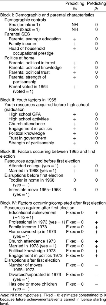
Table 1 lists the independent variables by temporal block and shows each variable's expected effect. The table has several notable features. First, the expected dissipation of effects of youth experiences is reflected in expected slopes of 0 for all pre-1968 measures on growth rate. Second, it is impossible for achievements occurring after 1968 to influence turnout in the 1968 election; therefore, all of these slopes are constrained to 0 a priori. Resources all have expected positive slopes. Disruptions occurring before the first eligible election are not expected to have any effects, but disruptions occurring later should lower turnout and this will be reflected in flatter growth rates (negative slopes).

RESULTS I: PARENTAL INFLUENCE ON INITIAL TURNOUT AND GROWTH
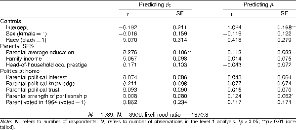
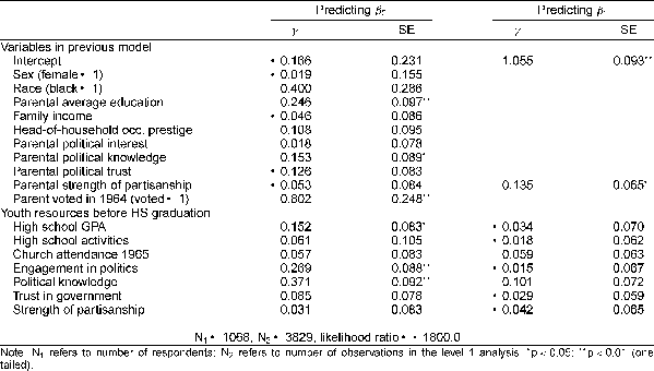
The initial model, reported in Table 2, includes sex, race, three measures of parental socioeconomic status, and five measures of parental political involvement including self-reported vote in the 1964 election. For each regressor, there are two estimated slopes: on β0 (reflecting the impact on starting level) and on β1 (the impact on growth). The intercept in the β0 column corresponds to γ00 in Eq. (3) and represents the log-odds of initial election turnout for a white male whose parent did not vote in the 1964 election and has the mean value for all SES and political variables (i.e., coded 0 for all 10 regressors). Similarly, the intercept in the equation predicting β1 represents an increase in the log-odds of turnout associated with each subsequent election [γ10 in Eq. (4)]. Thus the prediction equation for a white man (race and sex equal 0) from an average parental environment (all parental variables equal 0) with a nonvoting parent is
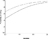
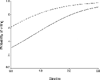
That is, the predicted odds of turnout in one's first election (when ELECTION and all other independent variables = 0), is e−0.192 (or 0.83 to 1), corresponding to a probability of about 0.45. To aid in interpreting the magnitudes of growth curve estimates, Eq. (7) is plotted as the lower curve in Fig. 1. This shows an initial turnout rate (intercept) of 45% and the familiar rise in turnout associated with age. The estimated growth rate of 1.024 represents the average rate of increase (in logged odds) in the sample.


Effect of Parents' Turnout on Offspring Turnout (- - - -) Those whose parents voted in 1964.(——) Those whose parents did not vote in 1964.
The estimates of γ in Table 2 show that neither sex, race, nor parental income achieve statistical significance. Parental education has a modest effect on their children's initial turnout, with a 1-unit change (i.e., one standard deviation) raising the intercept by about 0.28 so that the predicted probability of voting (for average youth with nonvoting parents) increases from 0.45 to 0.52.
The largest effect on initial turnout is parents' reported turnout. When all other variables are at the mean (or at 0 for sex and race), parents voting in 1964 increases the probability of initial turnout from 0.45 to 0.66. Thus, the 15% of parents who said that they did not vote leave their offspring substantially behind in the acquisition of the habit of voting. However, the convergence of the upper and lower curves in Fig. 1 shows that this disadvantage dissipates over time.
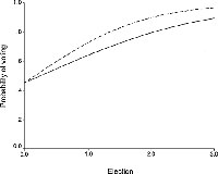
The estimates show that only one variable, parental strength of partisanship, has an impact on the slope β1. The magnitude of this effect is illustrated in Fig. 2 (which, again, holds other measures at 0). The effect is relatively small and mirrors Verba, Schlozman and Brady (1995, 449), who show that “politics in the home” at age 16 has a small direct effect on participation that is not explained away by a wide variety of SES, community, psychological, and resource measures. The finding raises the question of why this is the only parental resource whose influence does not dissipate over time.

Effect of Parents' Partisan Strength on Offspring Turnout (- - - -) Those whose parents were strong Republicans or strong Democrats.(——) Those whose parents were political independents.
To save space, this reported model includes both “structural” variables (demographics and status measures) and subjective/behavioral measures. A nested model including only structural variables shows that the total effect of education is about double the net effect (γ of 0.501 compared to 0.276). Thus half the total effect of parental education on initial turnout is mediated by parental political engagement, knowledge, and turnout.
To summarize the results so far, parental education and political knowledge each have modest effects on the probability of voting. Complementing these are two distinctly political variables, with parents' reported vote having a large impact on 1968 turnout and strength of partisanship providing a longer-term boost to turnout's growth rate. Measures of political alienation and engagement had no impact of any kind.
RESULTS II: HIGH SCHOOL INFLUENCES ON TURNOUT
This section explores achievements, activities, and psychological engagement in politics while respondents were high school seniors. The model reported in Table 3 retains from the first model both intercepts, all main effects, and one significant growth variable (parent's strength of partisanship) and adds the high school period measures. High school GPA is a rough measure of cognitive skill, work habits, and future socioeconomic success. It has a small and marginally significant (t = 1.82) impact on initial turnout. Our measure of high school student activities fails to achieve significance in either portion of the model.

Church attendance is consistently found to be a predictor of turnout in cross-sectional studies (e.g., Verba, Schlozman, and Brady 1995). Turnout scholars have never been entirely sure whether church involvement provides resources that have a causal impact on political participation or whether both are indicators of a general propensity to participate in community life. However, Table 3 shows that church attendance as a teenager in 1965 has no impact on turnout three years later or on the subsequent rate of growth.
The model also includes two measures of psychological engagement in politics. The first is a three-item engagement in politics scale, which is a standardized composite of expressed interest in politics and the frequency of both newspaper and newsmagazine readership. The second is the same six-item political knowledge scale that was administered to the parents. Both are significant predictors of 1968 turnout (but not subsequent rate of growth), and together they can have a fairly large effect. Being one standard deviation above the mean on both increases the log odds by 0.64, nearly as much as having a voting parent (illustrated in Fig. 3). Table 3 also shows that the effect of parental political knowledge drops by about 25%—implying that knowledgeable parents enhance turnout in part by fostering a similar attentiveness to public affairs in their children.

Effect of Engagement and Knowledge While in High School on Turnout (- - - -) Those 1 SD above the mean on political engagement and knowledge. (——) Those 1 SD below the mean on political engagement and knowledge.
Although not reported here, I inspected an intermediate model that included high school grades but excluded the political engagement measures and found the effect of GPA to be about 60% larger (γ = 0.244 compared to 0.152). None of the other structural variables showed noticeable changes. Thus high school achievement seems to matter but mostly indirectly through knowledge and political engagement.
None of the Block II variables, however, are significant in the β1 (slope) portion of the model. To ensure against Type II errors due to overspecification, the effects on growth were explored serially, with each variable entered alone to minimize multicollinearity. None achieved statistical significance, providing additional confidence for the idea that none of the high school period variables have lasting effects throughout the life course.
RESULTS III: LIFE EVENTS BETWEEN 1965 AND 1968
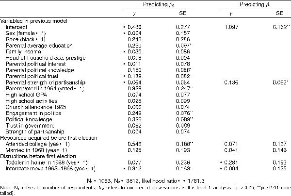
In this section, I examine the effects of four life transitions that occurred between the seniors' 1965 interview and their first eligible election. The next model adds dummy variables for having attended college (63% of the sample did so) and being married in 1968 (28%). The model also includes two variables hypothesized to have negative effects: being a parent in 1968 (15%) and whether or not the respondent made an interstate move between 1965 and 1968 (59%). Only two variables achieved statistical significance. Moving across state lines decreases the odds of voting by a small amount and is significant in a one-tailed test (t = −1.91). Attending college gives a substantial positive boost to initial turnout (about two thirds the size of the parental turnout effect illustrated in Fig. 1). The introduction of college attendance also causes the estimate for high school GPA to drop by more than 50% and its t value to drop below 1.00. Thus the small effect of high school grades appears to lead to a greater likelihood of college attendance, which directly affects turnout.
The model also shows that none of these variables achieves conventional levels of significance predicting growth. However, the lasting impact of being a parent is intriguing. The one-tailed probability is 0.07 and the coefficient estimate is negative and fairly large. In this sample, youth who became parents before the age of 22 start with no disadvantage but their rate of turnout growth is somewhat retarded.
Pre-1968 Factors: A Summary
Many events and social characteristics occurred or were fixed before the class of 1965 confronted its first election. Among these, having highly educated parents who voted in the 1964 election, being psychologically engaged with politics as high school seniors, and attending college boosted initial turnout, while mobility between 1965 and 1968 depressed it.
These findings supporting and clarify recent scholarship about education's role in political participation. Verba, Schlozman, and Brady (1995, 437–8) conclude that effects of parent's education are mediated largely by offspring's own socioeconomic status and interest in politics. Table 2 shows that parental education and political knowledge have no effect (neither direct nor indirect) on turnout growth. Their modest effects on initial turnout in the baseline model (γ's of 0.276 and 0.211) drop by only 25% (to γ's of 0.225 and 0.150, respectively) after accounting for offspring political engagement and college attendance (Table 4). Thus, the mechanism translating parental resources into children's initial political involvement is not captured by the variables in the model—perhaps because of poor specification (the transmission processes are captured by different variables entirely) or measurement error (high school grades and a simple indicator of college attendance may not adequately capture underlying variance in youth's educational achievements). One implication for cross-sectional studies, however, is that the effects of parental environment diminish over time and should, therefore, be modeled as interactions with age.

Among 21 pre-1968 variables, only parental strength of partisanship influenced turnout's rate of increase. Since partisanship is presumably a stable trait, the 1965 measure may be a reliable indicator of levels of partisanship many years in the future. Thus having partisan parents may accelerate the acquisition of knowledge and resources implicated in the lifelong learning process that underlies Rosenstone and Hansen's (1993) life experience approach.
RESULTS IV: LIFE EVENTS AFTER 1968
The fourth block includes measures at the heart of the life-cycle and life-experience explanations for turnout growth. All of these occurred after the 1968 election and, therefore, cannot have any effect on the initial probability of voting. Thus the effects of all subsequent variables will be modeled only as predictors of β1. We first model reports of events and behaviors and then add psychological measures to see if they mediate the effects of other variables.
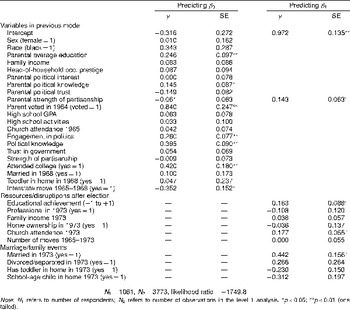
Table 5 reports a model that adds 10 structural variables measured in 1973 (about half a year after the cohort's second eligible election in November 1972). By now, most members have completed their education and are forming families and careers. The effects of three socioeconomic resources are generally consistent with the extant literature on turnout, which points to education as the most powerful component of SES with respect to turnout. Neither holding a professional position nor having a high income is significant but education has a sizable effect above and beyond the effect college attendance had on starting levels.

It is useful to see how the impact of education cumulates over the life course. The prediction equation for someone who never attended college (coded 0 for the 1968 dummy and coded −1 for the 1973 ordinal measure) who has values of 0 on all other variables is
For those who attained a college degree (coded 1 for both variables) the prediction equation is
These two growth curves are plotted in Fig. 4 and show that college education contributes to both a headstart and a more rapid rate of increase. Extrapolating beyond the range of the data gives a projection of a turnout gap of only 1% in three additional elections, when the typical respondent was 45 years old. Thus, the steeper slope does not prevent, but substantially delays, the point at which the less educated catch up. This supports Wolfinger and Rosenstone's (1980, 60) characterization that life experience can, over time, become a substitute for school. However, because this sample includes no respondents who lack a high school diploma, it is possible that those who dropped out of the class of 1965 never catch up with the college educated.

Effect of Education on Starting Levels and Growth Rates (- - - -) Those who never attended college. (——) Those who earned a bachelor's degree.
The next three variables—home ownership, geographic mobility, and church attendance—have been interpreted as tapping citizens's ties to their communities. These ties provide motivation to be informed and involved, as well as opportunities to gain political knowledge that reduce participation costs. Mobility may also raise the costs of maintaining registration (Squire, Wolfinger, and Glass 1987). Surprisingly, only frequency of church attendance in 1973 is a significant predictor of the growth rate. Unfortunately, this variable is measured right in the middle of the trajectories of most people. It is not possible to tell whether church involvement has a causal impact on turnout or whether both are indicators of a more general propensity to be involved in community life. At the very least, church attendance is a part of a dynamic complex of community involvements that includes voting.
Home Ownership and Mobility: Additional Considerations
Home ownership has long been regarded as an enhancer of turnout (e.g., Verba and Nie 1972, 139) and mobility a major barrier, but the estimates show that neither has an impact on growth rates. In each case the null findings could be (a) an artifact of the data and methods used here, (b) a peculiar characteristic of this particular cohort, or (c) a serious challenge to prior work.
The developmental model suggests that mobility effects will be greatest for habitual voters and, therefore, negligible for young voters and the estimates are consistent with that argument. Yet the possibility of an artifact is also high because the mobility measure is imprecise and stretches back to 1965. To get more leverage, I tried to replicate this finding using cross-sectional data from the American National Election Studies cumulative file (Miller and National Election Studies 1999). I pooled data from the same four presidential elections and estimated a model of turnout for four age groups. The youngest were 21–33 and correspond to the ages of those in the latent growth models. Table 6 reports the estimated slopes for geographic mobility, controlling for the year surveyed, age, race, education, sex, home ownership, family income, children in household, married, and folded party identification. The effect of mobility is substantively small and insignificant for young citizens and is large and significant for voters over 33 years old. These striking results provide strong corroboration that disruptions from mobility have an increasing impact throughout the life course. This conclusion suggests that an interaction with age may be the best way to specify the effects of mobility with cross-sectional data.

In contrast, pooled NES data (analysis not reported here but available on request) casts doubt on my estimates for the effect of home ownership; it has a robust effect at all age groups. After some exploration, I have concluded that the null effects here are probably due to a combination of factors—both substantive and methodological. First, home ownership is largely cumulative—most first time home owners continue to own homes for a long period thereafter—and therefore tracks closely with age and turnout. Thus, if unreliably measured, its true effects are likely to be absorbed by age or (in this research design) time.
Second, home ownership status changes very rapidly in the age range represented by our data. According to the Census's (1993) analysis of 1982 home ownership, only 19% of those under 25 owned a home but that number soars to 57% for those 30 to 34. Pooling Census data for a number of years (details available on request) shows the home ownership rate increases by 3.4% per year between age 21 and age 34. In 1973 38% of the sample reports owning a home and the Census data suggest that nearly 60% would own a home by the time of the 1980 election. Thus, the single measure has the benefit of being prior to voting outcomes but the corresponding disadvantage of being an extremely poor indicator of ownership status at the times of the last two elections. The null effects, combined with consistent and robust effects in cross-sectional studies, suggest that the positive impact of home ownership is probably immediate and therefore poorly captured by the developmental specification used here.
Family Life and Voter Turnout
The final set of objective variables measure aspects of family life: two dummy variables measuring marital status in 1973 and indicators of whether there are young children or school-age children in the household. The distinction between younger and older children derives from the idea that school-age children get parents involved in secondary associations such as the PTA and that schools provide a personal link to government policy. This implies that while very young children drain time and energy and lead to lower turnout, older children enhance networks that would result in greater political knowledge, mobilization, and an interest in outcomes. Taken together, these four variables paint a complex picture of the relationship between family life and turnout.
Although marriage when very young (most respondents were 22 or younger in 1968) had no effect on initial turnout, the same measure in 1973 had a substantial positive impact on turnout growth. In contrast, those who were married and divorced by 1973 (eight years after graduating from high school) had distinctively low growth rates (although the divorce measure does not achieve statistical significance, the two variables as a set improve the fit of the model). These growth rates, however, are higher than those of the never married—so divorce reverses only a portion of the marriage benefit. Yet, as Milbrath speculated, marriage is a mixed blessing for turnout because marriage is most often accompanied by children that erode about half the gain in turnout associated with marriage. Neither measure of the presence of children achieves significance and the two estimates are similar in magnitude. Given the similarity in effect estimates, I substituted a summary measure that simply indicates the presence of children. This did achieve significance (γ = 0.253, one-tailed p = 0.035) and is included in results reported in Table 7.

Psychological Engagement in Politics
Table 7 reports a model that adds the political engagement and political knowledge scales, both of which are significant predictors of turnout growth. Individually, the effects are modest but their combined impact can be substantial. Note also that the effect of education on growth is no longer statistically significant and the estimate has declined by about a third. Thus the two cognitive measures used here mediate about a third of the effect of higher education.
SUMMARY AND IMPLICATIONS
The developmental framework provides a new way to understand how resources and disruptions influence turnout in U.S. elections. When a cohort of young citizens becomes eligible to vote for the first time, parental socioeconomic and political resources largely determine who votes. Inertia ensures that parental resources continue to distinguish voters from nonvoters in succeeding elections. The influence of the parental resources, however, diminishes gradually as young adults' own accomplishments and status come to the fore. As the cohort ages, more and more members become habitual voters and the differences between the high- and the low-resource groups shrink. Among habitual voters, major life disruptions can interrupt the voting habit but only temporarily.
Analyses employing latent growth curve models and panel data produced results that are consistent with the general contours of the developmental theory. Table 4, for example, identifies seven significant predictors of initial turnout and none of these had an additional impact beyond the inertia that they helped to create.
Substantively, the most intriguing finding may be the enduring effect of parental partisanship, which speaks to how declining partisanship may contribute to long-term declines in turnout. If adults in their 30s, 40s, or 50s become disenchanted with parties, they tend to continue voting if that was their habit. However, the results suggest that their children will be slightly less likely to vote (perhaps decades later) as a consequence. To be sure, this cannot be the only long-term mechanism accounting for turnout decline but it could be a major one.
The findings also speak indirectly to issues concerning class bias of the electorate. High-SES parents pass on advantages to their children (both political behavior that children learn from and indirect gains through children's educational attainment). In the absence of other factors, these would lead to class bias of one cohort being reproduced in the next. However, as life expectancy increases, the gradual erosion of inherited advantages means that class bias may decline somewhat [as it may have done in recent decades (see Leighley and Nagler 1992)] because a larger portion of the electorate is at a life stage in which socioeconomic status matters little for turnout.
More generally, latent growth models should spur scholars toward better theories of the social bases of turnout. The simple conclusion that turnout is always a product of both starting level and growth rate (each with rather different predictors) is itself important and should lead to new questions about turnout, which, in turn, should produce better hypotheses and a cumulation of new findings. A major limitation, of course, is the dearth of appropriate longitudinal data. In this regard, the completion of a fourth wave of the Student–Parent Socialization Study and its release to the larger community in coming years can only mean good news for the study of political behavior over the life course. However, as illustrated in my supplemental analysis of geographic mobility, careful use of age × resource and age × disruption interactions should allow tests of some developmental hypotheses with cross-sectional data.
Finally, latent growth curve models may have wider applicability in political science. Whenever theory or previous research suggests a monotonic trend of growth or decline, this approach allows asking “time series questions” even when the number of time points is as few as three or four. As such, applications of this method may extend to such diverse phenomena as the life cycles of social movements, the escalation phase of arms races, economic growth in developing nations, transitions to democracy, and various diffusion processes. Thus, in many areas of inquiry, growth models have the potential to bring theory and empirical analysis into closer alignment.
APPENDIX: FREQUENCIES AND TREATMENT OF MISSING DATA FOR THE DEPENDENT VARIABLE

Among all youth interviewed in 1965 this paper's analysis is based on those who were 21 years old at the time of the 1968 general election. Among these, 1153 responded to at least one of the four turnout questions. The marginal distribution for the four turnout measures is presented in Table A1.
The Bayesian estimation method of random effects models means that “both the number of observations per person and the spacing of observations may vary” (Bryk and Raudenbush 1992, 133). That is, any respondent who has a valid turnout code for at least one election can be included in the analysis, maximizing the amount of information used in generating the parameter estimates. The nature of Bayesian estimators is such that individuals with more data points are weighted more heavily. As a result, the number of usable observations—designated as N1 in all tables—exceeds the 862 respondents who have valid data for all four elections. N2 in the tables refers to the total number of valid turnout codes, which is N2 = [sum ](ki), where ki is the number of valid data points for the ith respondent.
This research was supported in part by the Character and Competence Program of the Alfred E. Murray Research Center and by the Research and Graduate Studies Office of Penn State's College of the Liberal Arts. I thank Christopher Reenock, Andrew Shults, and Nancy Wiefek for their research assistance and Don Hedeker for statistical and software advice. Lee Ann Banaszak, Suzanna DeBoef, Michael Guge, Ben Highton, Quan Li, Jeff Manza, Nancy Wiefek, Susan Welch, and several anonymous reviewers provided helpful comments on early versions of this paper. Michael Guge deserves special thanks for first encouraging me to examine latent growth curve analysis. Data analyzed in the paper were originally collected by M. Kent Jennings, Richard Niemi, and Gregory Markus and distributed for secondary analysis by the Inter-university Consortium for Political and Social Research.
References
Aldrich John H.
1993
Rational Choice and Turnout
American Journal of Political Science
37
February
246 78Google Scholar
Bryk Anthony S.
Raudenbush Stephen W.
1992
Hierarchical Linear Models
Beverly Hills, CA
Sage
Campbell Angus
Converse Philip E.
Miller Warren E.
Stokes Donald E.
1960
The American Voter
New York
Wiley
Center for Political Studies
2000
American National Election Series: 1972, 1974, 1976
[computer file]. (Study 7607) Conducted by University of Michigan, Center for Political Studies. 3rd ICPSR ed. Ann Arbor, MI: Inter-university Consortium for Political and Social Research [producer and distributor]
Hedeker Donald
Gibbons Robert P.
1994
A Random-Effects Ordinal Regression Model for Multivariate Analysis
Biometrics
50
December
933 44Google Scholar
Hedeker Donald
Gibbons Robert P.
1996
MIXOR: A Computer Program for Mixed-Effects Ordinal Probit and Logistic Regression Analysis
software manual
Chicago
University of Illinois at Chicago School of Public Health
Highton Benjamin
Wolfinger Raymond E.
2001
The First Seven Years of the Political Life Cycle
American Journal of Political Science
45
January
202 9Google Scholar
Jankowski Thomas B.
2001
The Aging American Voter: Changes in Participation Over the Life Span
Paper presented at the Annual Meetings of the Midwest Political Science Association, Chicago, April 19–22
Jennings M. Kent
1972
Student–Parent Socialization Study, 1965
[computer file] (Study 7286) Conducted by M. Kent Jennings, University of Michigan. ICPSR ed. Ann Arbor, MI: Inter-university Consortium for Political and Social Research [producer and distributor]
Jennings M. Kent
Markus Gregory B.
1988
Political Involvement in Later Years: A Longitudinal Survey
American Journal of Political Science
32
May
302 16Google Scholar
Jennings M. Kent
Niemi Richard
1981
Generations and Politics
Princeton, NJ
Princeton University Press
Jennings M. Kent
Niemi Richard G.
1991
The Youth–Parent Socialization Panel Study, 1965–1973
[computer file] (Study 7779). Conducted by University of Michigan, Center for Political Studies. 2nd ICPSR ed. Ann Arbor, MI: Inter-university Consortium for Political and Social Research [producer and distributor]
Jennings M. Kent
Markus Gregory B.
Niemi Richard G.
1991
Youth–Parent Socialization Panel Study, 1965–1982: Wave III
[computer file] (Study 9134) Conducted by University of Michigan, Center for Political Studies/Survey Research Center. 3rd ICPSR ed. Ann Arbor, MI: Inter-university Consortium for Political and Social Research [producer and distributor]
Leighley Jan E.
Nagler Jonathan
1992
Socioeconomic Class Bias in Turnout, 1964–1988: The Voters Remain the Same
American Political Science Review
86
September
725 36Google Scholar
Lieberson Stanley
1985
Making It Count: The Improvement of Social Research and Theory
Berkeley
University of California Press
Milbrath Lester W.
1965
Political Participation
Chicago
Rand McNally
Miller Warren E.
National Election Studies
1999
American National Election Studies Cumulative Data File, 1948–1998
[computer file] (Study 8475), 10th ICPSR version. Ann Arbor: University of Michigan, Center for Political Studies [producer], Inter-university Consortium for Political and Social Research [distributor]
Miller Warren E.
Shanks J. Merrill
1996
The New American Voter
Cambridge, MA
Harvard University Press
Plutzer Eric
1998
Family Structure and the Political Participation of African American Women
The Development of Character and Competence Through Life
Anne Colby
Jacqueline James
Daniel Hart
Chicago
University of Chicago Press
Riley Matilda White
1973
Aging and Cohort Succession: Interpretations and Misinterpretations
Public Opinion Quarterly
37
Spring
35
49Google Scholar
Rosenstone Steven J.
1982
Economic Adversity and Voter Turnout
American Journal of Political Science
26
February
25
46Google Scholar
Rosenstone Steven J.
Hansen John Mark
1993
Mobilization, Participation, and Democracy in America
New York
Macmillan
Searing Donald D.
Schwartz Joel J.
Lind Alden E.
1973
The Structuring Principle: Political Socialization and Belief Systems
American Political Science Review
67
June
415 32Google Scholar
Squire Peverill
Wolfinger Raymond
Glass David
1987
Residential Mobility and Voter Turnout
American Political Science Review
81
March
45
65Google Scholar
Stoker Laura
Jennings M. Kent
1995
Life-Cycle Transitions and Political Participation: The Case of Marriage
American Political Science Review
89
June
421 33Google Scholar
Strate John M.
Parrish Charles M.
Elder Charles D.
Ford IIICoit
1989
Life Span Civic Development and Voting Participation
American Political Science Review
83
June
443 64Google Scholar
Timpone Richard J.
1998
Structure, Behavior, and Voter Turnout in the United States
American Political Science Review
92
March
145 58Google Scholar
United States Bureau of the Census
1993
First-Time Homeowners in 1989: A Comparative Perspective
Current Housing Reports
H121/93-1
Verba Sidney
Nie Norman
1972
Participation in America
New York
Harper and Row
Verba Sidney
Schlozman Kay Lehman
Brady Henry
1995
Voice and Equality: Civic Voluntarism in American Politics
Cambridge, MA
Harvard University Press
Wolfinger Raymond
Rosenstone Steven J.
1980
Who Votes
New Haven, CT
Yale University Press
Zipp John F.
Smith Joel
1979
The Structure of Electoral Political Participation
American Journal of Sociology
85
July
167 77Google Scholar
Summary of Independent Variables and Their Hypothesized Effects
The Effects of Parent SES and Parent Political Involvement on Starting Level and Growth
(- - - -) Those whose parents voted in 1964.(——) Those whose parents did not vote in 1964.
(- - - -) Those whose parents were strong Republicans or strong Democrats.(——) Those whose parents were political independents.
The Effects of High School Resources and Accomplishments on Starting Level and Growth
(- - - -) Those 1 SD above the mean on political engagement and knowledge. (——) Those 1 SD below the mean on political engagement and knowledge.
The Effects of Life Events Between High School and First Election on Starting Levels and Growth
The Effects of Life Events After the First Election on Turnout Growth
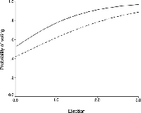
(- - - -) Those who never attended college. (——) Those who earned a bachelor's degree.
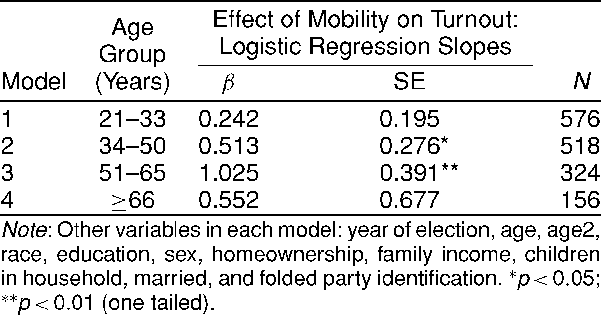
Effect of Geographic Mobility on Turnout in Presidential Elections, by Age Group (Subset of NES Cummulative File: 1968 through 1980, High School Graduates)
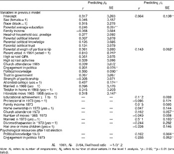
Final Model Predicting Starting Level and Turnout Growth, Including 1973 Political Knowledge and Engagement
 You have Access
- 659
- Cited by
Comments
No Comments have been published for this article.