2.1 Schematic representation and governing equations

Figure 1.

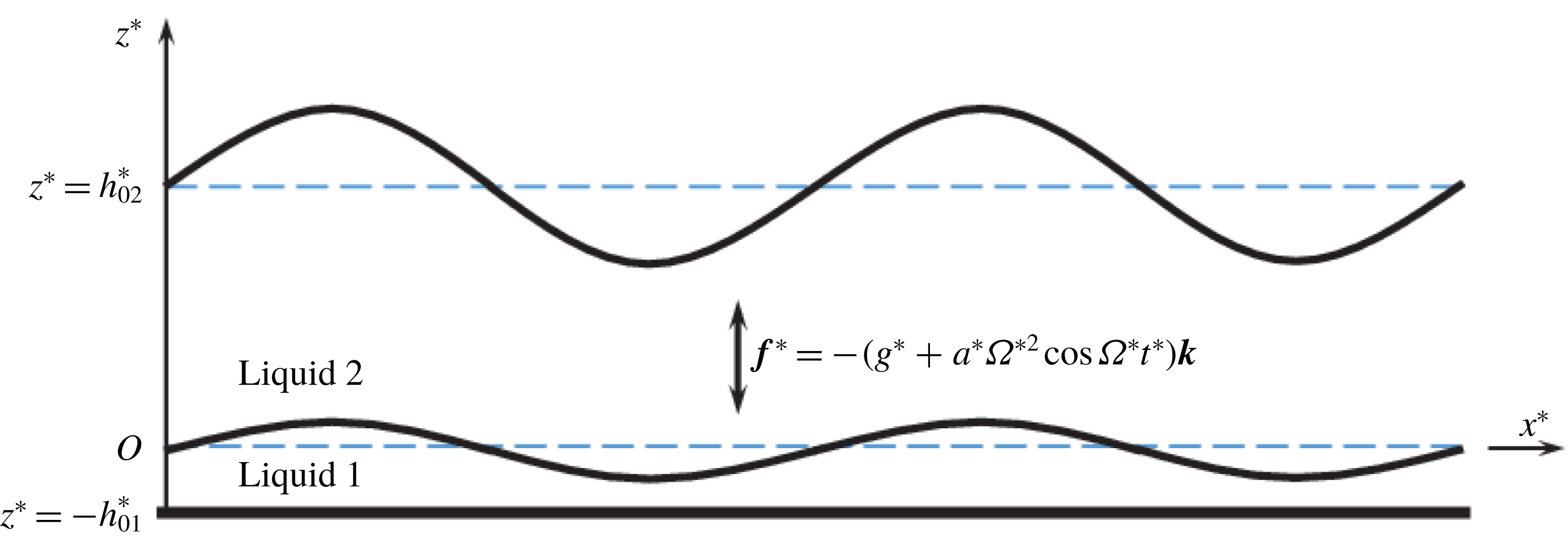
Schematic configuration of the system.

As shown schematically by figure 1, a conjugated double-layer system of two immiscible Newtonian and incompressible liquids is considered. The top layer, consisting of a liquid (indexed by 2) with density $\unicode[STIX]{x1D70C}_{2}^{\ast }$ and kinematic viscosity $\unicode[STIX]{x1D708}_{2}^{\ast }$ , is much thicker than the bottom one, which consists of a liquid (indexed by 1) with density $\unicode[STIX]{x1D70C}_{1}^{\ast }$ and viscosity $\unicode[STIX]{x1D708}_{1}^{\ast }$ . The superscript $\ast$ denotes dimensional variables. A Cartesian coordinate system with unit vectors ( $\boldsymbol{i},\boldsymbol{j},\boldsymbol{k}$ ) and origin $O$ is introduced, where $x$ and $y$ span the horizontal plane, representing the undisturbed interface between the two layers. The interfacial tension is denoted by $\unicode[STIX]{x1D70E}_{1}^{\ast }$ . In our description, the vertical axis $z$ is antiparallel to the gravitational acceleration vector $\boldsymbol{g}^{\ast }=-g^{\ast }\boldsymbol{k}$ . The top free surface in its undeformed state is located at $z^{\ast }=h_{02}^{\ast }$ , and its surface tension is denoted by $\unicode[STIX]{x1D70E}_{2}^{\ast }$ . The subscript $0$ represents the base state. The rigid substrate is placed at $z^{\ast }=-h_{01}^{\ast }$ . The whole system is exposed to a time-periodic acceleration $\boldsymbol{f}^{\ast }=-(g^{\ast }+a^{\ast }\unicode[STIX]{x1D6FA}^{\ast 2}\cos \unicode[STIX]{x1D6FA}^{\ast }t^{\ast })\boldsymbol{k}$ , where $a^{\ast }$ denotes the amplitude of the oscillation, $\unicode[STIX]{x1D6FA}^{\ast }/2\unicode[STIX]{x03C0}$ the angular frequency and $t^{\ast }$ the time. For the sake of compactness, the acceleration amplitude $a^{\ast }\unicode[STIX]{x1D6FA}^{\ast 2}$ is denoted by  $A^{\ast }$ .

The velocity is denoted by $\boldsymbol{v}_{i}^{\ast }=\boldsymbol{u}_{i}^{\ast }+w_{i}^{\ast }\boldsymbol{k}$ , the pressure by $p_{i}^{\ast }$ , while the subscript $i=1,2$ references the different layers. Accordingly, the Newtonian and incompressible Navier–Stokes equations governing the flow inside the two layers read

(2.1) $$\begin{eqnarray}\displaystyle \unicode[STIX]{x1D735}_{s}^{\ast }\boldsymbol{\cdot }\boldsymbol{u}_{i}^{\ast }+\frac{\unicode[STIX]{x2202}w_{i}^{\ast }}{\unicode[STIX]{x2202}z^{\ast }}=0, & & \displaystyle\end{eqnarray}$$

(2.2) $$\begin{eqnarray}\displaystyle \frac{\unicode[STIX]{x2202}\boldsymbol{v}_{i}^{\ast }}{\unicode[STIX]{x2202}t^{\ast }}+\boldsymbol{u}_{i}^{\ast }\boldsymbol{\cdot }\unicode[STIX]{x1D735}_{s}^{\ast }\boldsymbol{v}_{i}^{\ast }+w_{i}^{\ast }\frac{\unicode[STIX]{x2202}\boldsymbol{v}_{i}^{\ast }}{\unicode[STIX]{x2202}z^{\ast }} & = & \displaystyle -\frac{1}{\unicode[STIX]{x1D70C}_{i}^{\ast }}\left(\unicode[STIX]{x1D735}_{s}^{\ast }+\boldsymbol{k}\frac{\unicode[STIX]{x2202}}{\unicode[STIX]{x2202}z^{\ast }}\right)p_{i}^{\ast }-[g^{\ast }+a^{\ast }\unicode[STIX]{x1D6FA}^{\ast 2}\cos (\unicode[STIX]{x1D6FA}^{\ast }t^{\ast })]\boldsymbol{k}\nonumber\\ \displaystyle & & \displaystyle +\,\unicode[STIX]{x1D708}_{i}^{\ast }\left({\unicode[STIX]{x1D6FB}_{s}^{\ast }}^{2}\boldsymbol{v}_{i}^{\ast }+\frac{\unicode[STIX]{x2202}^{2}\boldsymbol{v}_{i}^{\ast }}{\unicode[STIX]{x2202}{z^{\ast }}^{2}}\right),\end{eqnarray}$$

where the horizontal gradient operator is defined by $\unicode[STIX]{x1D735}_{s}^{\ast }=\boldsymbol{i}\unicode[STIX]{x2202}/\unicode[STIX]{x2202}x^{\ast }+\boldsymbol{j}\unicode[STIX]{x2202}/\unicode[STIX]{x2202}y^{\ast }$ . At the rigid substrate at the bottom, the no-slip and the no-penetration boundary conditions are chosen. Mathematically, this is expressed by

(2.3) $$\begin{eqnarray}\displaystyle z^{\ast }=-h_{01}^{\ast }:\quad \boldsymbol{u}_{1}^{\ast }=w_{1}^{\ast }=0. & & \displaystyle\end{eqnarray}$$

At the deformable interface between the two layers $z^{\ast }=h_{1}^{\ast }(x^{\ast },y^{\ast },t^{\ast })-h_{01}^{\ast }$ , the boundary conditions are

(2.4) $$\begin{eqnarray}\displaystyle & \displaystyle \frac{\unicode[STIX]{x2202}h_{1}^{\ast }}{\unicode[STIX]{x2202}t^{\ast }}+\boldsymbol{u}_{1}^{\ast }\boldsymbol{\cdot }\unicode[STIX]{x1D735}_{s}^{\ast }h_{1}^{\ast }=w_{1}^{\ast }, & \displaystyle\end{eqnarray}$$

(2.5) $$\begin{eqnarray}\displaystyle & \displaystyle \boldsymbol{v}_{1}^{\ast }=\boldsymbol{v}_{2}^{\ast }, & \displaystyle\end{eqnarray}$$

(2.6) $$\begin{eqnarray}\displaystyle & \displaystyle -(\unicode[STIX]{x1D64B}^{\ast }\boldsymbol{\cdot }\boldsymbol{n}\boldsymbol{\cdot }\boldsymbol{n})_{2}+(\unicode[STIX]{x1D64B}^{\ast }\boldsymbol{\cdot }\boldsymbol{n}\boldsymbol{\cdot }\boldsymbol{n})_{1}=2\unicode[STIX]{x1D70E}_{1}^{\ast }H_{1}^{\ast }, & \displaystyle\end{eqnarray}$$

(2.7) $$\begin{eqnarray}\displaystyle & \displaystyle -(\unicode[STIX]{x1D64B}^{\ast }\boldsymbol{\cdot }\boldsymbol{n}\boldsymbol{\cdot }\unicode[STIX]{x1D749})_{2}+(\unicode[STIX]{x1D64B}^{\ast }\boldsymbol{\cdot }\boldsymbol{n}\boldsymbol{\cdot }\unicode[STIX]{x1D749})_{1}=0, & \displaystyle\end{eqnarray}$$

which include the kinematic relation, continuity of the velocities, viscous shear stress continuity and the normal stress jump. The mean curvature is denoted by $H_{i}^{\ast }$ , the normal and tangential unit vectors are given by $\boldsymbol{n}$ and $\unicode[STIX]{x1D749}$ , and $\unicode[STIX]{x1D64B}_{i}^{\ast }$ denotes the viscous stress tensors. The detailed expressions are given by

(2.8) $$\begin{eqnarray}\displaystyle \left.\begin{array}{@{}c@{}}\displaystyle \boldsymbol{n}_{i}=\frac{-\unicode[STIX]{x1D735}_{s}^{\ast }h_{i}^{\ast }+\boldsymbol{k}}{(1+|\unicode[STIX]{x1D735}_{s}^{\ast }h_{i}^{\ast }|^{2})^{1/2}},\quad \unicode[STIX]{x1D749}_{i}=\frac{-\unicode[STIX]{x1D735}_{s}^{\ast }h_{i}^{\ast }-|\unicode[STIX]{x1D735}_{s}^{\ast }h_{i}^{\ast }|^{2}\boldsymbol{k}}{|\unicode[STIX]{x1D735}_{s}^{\ast }h_{i}^{\ast }|\cdot (1+|\unicode[STIX]{x1D735}_{s}^{\ast }h_{i}^{\ast }|^{2})^{1/2}},\\ \displaystyle H_{i}^{\ast }=-\frac{1}{2}\unicode[STIX]{x1D735}_{s}^{\ast }\boldsymbol{\cdot }\left[\frac{-\unicode[STIX]{x1D735}_{s}^{\ast }h_{i}^{\ast }+\boldsymbol{k}}{(1+|\unicode[STIX]{x1D735}_{s}^{\ast }h_{i}^{\ast }|^{2})^{1/2}}\right],\\ \displaystyle \unicode[STIX]{x1D64B}_{i}^{\ast }=-p_{i}^{\ast }\unicode[STIX]{x1D644}+\unicode[STIX]{x1D70C}_{i}^{\ast }\unicode[STIX]{x1D708}_{i}^{\ast }\left\{\!\left(\unicode[STIX]{x1D735}_{s}^{\ast }+\boldsymbol{k}\frac{\unicode[STIX]{x2202}}{\unicode[STIX]{x2202}z^{\ast }}\right)(\boldsymbol{u}_{i}^{\ast }+\boldsymbol{k}w_{i}^{\ast })+\left[\left(\unicode[STIX]{x1D735}_{s}^{\ast }+\boldsymbol{k}\frac{\unicode[STIX]{x2202}}{\unicode[STIX]{x2202}z^{\ast }}\right)(\boldsymbol{u}_{i}^{\ast }+\boldsymbol{k}w_{i}^{\ast })\right]^{\text{T}}\right\}\!.\end{array}\right\} & & \displaystyle \nonumber\\ \displaystyle & & \displaystyle\end{eqnarray}$$

At the top free surface $z^{\ast }=h_{2}^{\ast }(x^{\ast },y^{\ast },t^{\ast })$ , the boundary conditions are given by

(2.9) $$\begin{eqnarray}\displaystyle & \displaystyle \frac{\unicode[STIX]{x2202}h_{2}^{\ast }}{\unicode[STIX]{x2202}t^{\ast }}+\boldsymbol{u}_{2}^{\ast }\boldsymbol{\cdot }\unicode[STIX]{x1D735}_{s}^{\ast }h_{2}^{\ast }=w_{2}^{\ast }, & \displaystyle\end{eqnarray}$$

(2.10) $$\begin{eqnarray}\displaystyle & \displaystyle (\unicode[STIX]{x1D64B}^{\ast }\boldsymbol{\cdot }\boldsymbol{n}\boldsymbol{\cdot }\boldsymbol{n})_{2}=2\unicode[STIX]{x1D70E}_{2}^{\ast }H_{2}^{\ast }, & \displaystyle\end{eqnarray}$$

(2.11) $$\begin{eqnarray}\displaystyle & \displaystyle (\unicode[STIX]{x1D64B}^{\ast }\boldsymbol{\cdot }\boldsymbol{n}\boldsymbol{\cdot }\unicode[STIX]{x1D749})_{2}=0, & \displaystyle\end{eqnarray}$$

which neglect the influence from the surroundings.

Non-dimensionalization is carried out as follows:

(2.12) $$\begin{eqnarray}\displaystyle \left.\begin{array}{@{}c@{}}\displaystyle (x^{\ast },y^{\ast },z^{\ast },h_{2}^{\ast },h_{1}^{\ast },a^{\ast })=h_{02}^{\ast }(x_{2},y_{2},z_{2},h_{2},hh_{1},a_{2})=h_{01}^{\ast }\left(x_{1},y_{1},z_{1},\frac{1}{h}h_{2},h_{1},a_{1}\right),\\ \displaystyle \boldsymbol{v}_{2}^{\ast }=h_{02}^{\ast }\unicode[STIX]{x1D6FA}^{\ast }\boldsymbol{v}_{2},\quad \unicode[STIX]{x1D735}_{s}^{\ast }=\frac{1}{h_{02}^{\ast }}\unicode[STIX]{x1D735}_{2}=\frac{1}{h_{01}^{\ast }}\unicode[STIX]{x1D735}_{1},\quad \boldsymbol{v}_{1}^{\ast }=\frac{\unicode[STIX]{x1D708}_{1}^{\ast }}{h_{01}^{\ast }}\boldsymbol{v}_{1},\quad \unicode[STIX]{x1D6FA}^{\ast }=\frac{\unicode[STIX]{x1D708}_{1}^{\ast }}{{h_{01}^{\ast }}^{2}}\unicode[STIX]{x1D6FA}_{1},\\ \displaystyle (\unicode[STIX]{x1D64B}^{\ast },p^{\ast })=\unicode[STIX]{x1D70C}_{2}^{\ast }(h_{02}^{\ast }\unicode[STIX]{x1D6FA}^{\ast })^{2}(\unicode[STIX]{x1D64B}_{2},p_{2})=\unicode[STIX]{x1D70C}_{1}^{\ast }\left(\frac{\unicode[STIX]{x1D708}_{1}^{\ast }}{h_{01}^{\ast }}\right)^{2}(\unicode[STIX]{x1D64B}_{1},p_{1}),\quad t^{\ast }=\frac{1}{\unicode[STIX]{x1D6FA}^{\ast }}t_{2}=\frac{{h_{01}^{\ast }}^{2}}{\unicode[STIX]{x1D708}_{1}^{\ast }}t_{1},\end{array}\right\} & & \displaystyle \nonumber\\ \displaystyle & & \displaystyle\end{eqnarray}$$

where $h=h_{01}^{\ast }/h_{02}^{\ast }$ is always sufficiently small. The scales above are introduced in such a way that the dimensionless variables are $O(1)$ , considering the disparity between the two layers. The velocity scale in the upper layer is an advective scale, with the oscillation period as time scale. For the lower layer, considering the dominance of viscous forces, a diffusive scale for the velocity was chosen, based on the time scale for momentum diffusion. The scales and the dimensionless groups resulting from these are further discussed at the end of this section.

To simplify the original Navier–Stokes equation to a thin-film evolution equation, the long-wavelength approximation is applied to the bottom layer. Based on the normal perturbation scheme, the velocity is expanded in $h$ up to $O(h^{1})$ according to

(2.13) $$\begin{eqnarray}\displaystyle \boldsymbol{u}_{1}=\boldsymbol{u}_{1}^{(0)}+h\boldsymbol{u}_{1}^{(1)}+\cdots \,,\quad \tilde{w}_{1}=\tilde{w}_{1}^{(0)}+h\tilde{w}_{1}^{(1)}+\cdots \,, & & \displaystyle\end{eqnarray}$$

where $w_{1}=h\tilde{w}_{1}$ , and the superscripts denote the expansion orders. More details are given in appendix A. Finally, the complete form of the dimensionless governing equations for the whole system can be summarized by

(2.14) $$\begin{eqnarray}\displaystyle \unicode[STIX]{x1D735}_{2}\boldsymbol{\cdot }\boldsymbol{u}_{2}+\frac{\unicode[STIX]{x2202}w_{2}}{\unicode[STIX]{x2202}z_{2}} & = & \displaystyle 0,\end{eqnarray}$$

(2.15) $$\begin{eqnarray}\displaystyle \frac{\unicode[STIX]{x2202}\boldsymbol{v}_{2}}{\unicode[STIX]{x2202}t_{2}}+\boldsymbol{u}_{2}\boldsymbol{\cdot }\unicode[STIX]{x1D735}_{2}\boldsymbol{v}_{2}+w_{2}\frac{\unicode[STIX]{x2202}\boldsymbol{v}_{2}}{\unicode[STIX]{x2202}z_{2}} & = & \displaystyle -\left(\unicode[STIX]{x1D735}_{2}+\boldsymbol{k}\frac{\unicode[STIX]{x2202}}{\unicode[STIX]{x2202}z_{2}}\right)p_{2}-\left(\frac{1}{Fr_{2}^{2}}+a_{2}\cos t_{2}\right)\boldsymbol{k}\nonumber\\ \displaystyle & & \displaystyle +\,\frac{1}{Re_{2}}\left({\unicode[STIX]{x1D735}_{2}}^{2}\boldsymbol{v}_{2}+\frac{\unicode[STIX]{x2202}^{2}\boldsymbol{v}_{2}}{\unicode[STIX]{x2202}{z_{2}}^{2}}\right).\end{eqnarray}$$

The following boundary/interfacial conditions apply. At the upper free surface $z_{2}=h_{2}(x_{2},y_{2},t_{2})$ :

(2.16) $$\begin{eqnarray}\displaystyle \frac{\unicode[STIX]{x2202}h_{2}}{\unicode[STIX]{x2202}t_{2}}+\boldsymbol{u}_{2}\boldsymbol{\cdot }\unicode[STIX]{x1D735}_{2}h_{2}=w_{2}, & & \displaystyle\end{eqnarray}$$

(2.17) $$\begin{eqnarray}\displaystyle & & \displaystyle \frac{\unicode[STIX]{x2202}\boldsymbol{u}_{2}}{\unicode[STIX]{x2202}z_{2}}+\unicode[STIX]{x1D735}_{2}w_{2}-[\unicode[STIX]{x1D735}_{2}\boldsymbol{u}_{2}+(\unicode[STIX]{x1D735}_{2}\boldsymbol{u}_{2})^{\text{T}}]\boldsymbol{\cdot }\unicode[STIX]{x1D735}_{2}h_{2}\nonumber\\ \displaystyle & & \displaystyle \quad +\left[2\frac{\unicode[STIX]{x2202}w_{2}}{\unicode[STIX]{x2202}z_{2}}-\left(\frac{\unicode[STIX]{x2202}\boldsymbol{u}_{2}}{\unicode[STIX]{x2202}z_{2}}+\unicode[STIX]{x1D735}_{2}w_{2}\right)\boldsymbol{\cdot }\unicode[STIX]{x1D735}_{2}h_{2}\right]\unicode[STIX]{x1D735}_{2}h_{2}=0,\end{eqnarray}$$

(2.18) $$\begin{eqnarray}\displaystyle & & \displaystyle p_{2}+\frac{1}{We_{2}}\unicode[STIX]{x1D735}_{2}\boldsymbol{\cdot }\left[\frac{\unicode[STIX]{x1D735}_{2}h_{2}}{(1+|\unicode[STIX]{x1D735}_{2}h_{2}|^{2})^{1/2}}\right]\nonumber\\ \displaystyle & & \displaystyle \quad =\frac{1}{Re_{2}}(1+|\unicode[STIX]{x1D735}_{2}h_{2}|^{2})^{-1}\left\{2\frac{\unicode[STIX]{x2202}w_{2}}{\unicode[STIX]{x2202}z_{2}}-2\left(\frac{\unicode[STIX]{x2202}\boldsymbol{u}_{2}}{\unicode[STIX]{x2202}z_{2}}+\unicode[STIX]{x1D735}_{2}w_{2}\right)\boldsymbol{\cdot }\unicode[STIX]{x1D735}_{2}h_{2}\right.\nonumber\\ \displaystyle & & \displaystyle \qquad +\left.\unicode[STIX]{x1D735}_{2}h_{2}\boldsymbol{\cdot }[\unicode[STIX]{x1D735}_{2}\boldsymbol{u}_{2}+(\unicode[STIX]{x1D735}_{2}\boldsymbol{u}_{2})^{\text{T}}]\boldsymbol{\cdot }\unicode[STIX]{x1D735}_{2}h_{2}\right\}.\end{eqnarray}$$

At the liquid–liquid interface $z_{1}=h_{1}-1$ or $z_{2}=h(h_{1}-1)$ :

(2.19) $$\begin{eqnarray}\displaystyle \frac{\unicode[STIX]{x2202}h_{1}}{\unicode[STIX]{x2202}\tilde{t}_{1}} & = & \displaystyle \frac{1}{3}\tilde{\unicode[STIX]{x1D735}}_{1}\boldsymbol{\cdot }\{[(G_{1}+\tilde{a}_{1}\tilde{\unicode[STIX]{x1D6FA}}_{1}^{2}\cos \tilde{\unicode[STIX]{x1D6FA}}_{1}\tilde{t}_{1})\tilde{\unicode[STIX]{x1D735}}_{1}h_{1}-\tilde{S}_{1}\tilde{\unicode[STIX]{x1D6FB}}_{1}^{3}h_{1}]h_{1}^{3}\}\nonumber\\ \displaystyle & & \displaystyle -\,\frac{h}{2\unicode[STIX]{x1D70C}\unicode[STIX]{x1D708}^{2}}Re_{2}\tilde{\unicode[STIX]{x1D735}}_{1}\boldsymbol{\cdot }\left[h_{1}^{2}\left.\left(\frac{\unicode[STIX]{x2202}\boldsymbol{u}_{2}}{\unicode[STIX]{x2202}z_{2}}+\unicode[STIX]{x1D735}_{2}w_{2}\right)\right|_{z_{1}=h_{1}-1}\right],\end{eqnarray}$$

(2.20) $$\begin{eqnarray}\displaystyle \boldsymbol{u}_{2} & = & \displaystyle \frac{\unicode[STIX]{x1D708}}{Re_{2}}\boldsymbol{u}_{1}^{(1)},\quad w_{2}=\frac{h\unicode[STIX]{x1D708}}{Re_{2}}\tilde{w}_{1}^{(1)},\end{eqnarray}$$

(2.21) $$\begin{eqnarray}\displaystyle \boldsymbol{u}_{1}^{(0)} & = & \displaystyle \tilde{w}_{1}^{(0)}=0,\end{eqnarray}$$

(2.22) $$\begin{eqnarray}\displaystyle \boldsymbol{u}_{1}^{(1)} & = & \displaystyle -\frac{1}{2}[(G_{1}+\tilde{a}_{1}\tilde{\unicode[STIX]{x1D6FA}}_{1}^{2}\cos \tilde{\unicode[STIX]{x1D6FA}}_{1}\tilde{t}_{1})\tilde{\unicode[STIX]{x1D735}}_{1}h_{1}-\tilde{S}_{1}\tilde{\unicode[STIX]{x1D6FB}}_{1}^{3}h_{1}]h_{1}^{2}\nonumber\\ \displaystyle & & \displaystyle +\,\frac{h}{\unicode[STIX]{x1D70C}\unicode[STIX]{x1D708}^{2}}Re_{2}h_{1}\left.\left(\frac{\unicode[STIX]{x2202}\boldsymbol{u}_{2}}{\unicode[STIX]{x2202}z_{2}}+\unicode[STIX]{x1D735}_{2}w_{2}\right)\right|_{z_{1}=h_{1}-1},\end{eqnarray}$$

(2.23) $$\begin{eqnarray}\displaystyle \tilde{w}_{1}^{(1)} & = & \displaystyle (G_{1}+\tilde{a}_{1}\tilde{\unicode[STIX]{x1D6FA}}_{1}^{2}\cos \tilde{\unicode[STIX]{x1D6FA}}_{1}\tilde{t}_{1})\left[-\frac{1}{6}h_{1}^{3}\tilde{\unicode[STIX]{x1D6FB}}_{1}^{2}h_{1}+\frac{1}{2}h_{1}^{2}\tilde{\unicode[STIX]{x1D735}}_{1}\boldsymbol{\cdot }(h_{1}\tilde{\unicode[STIX]{x1D735}}_{1}h_{1})\right]\nonumber\\ \displaystyle & & \displaystyle +\,\tilde{S}_{1}\left[\frac{1}{6}h_{1}^{3}\tilde{\unicode[STIX]{x1D6FB}}_{1}^{4}h_{1}-\frac{1}{2}h_{1}^{2}\tilde{\unicode[STIX]{x1D735}}_{1}\boldsymbol{\cdot }(h_{1}\tilde{\unicode[STIX]{x1D6FB}}_{1}^{3}h_{1})\right]\nonumber\\ \displaystyle & & \displaystyle -\,\frac{h}{2\unicode[STIX]{x1D70C}\unicode[STIX]{x1D708}^{2}}Re_{2}h_{1}^{2}\tilde{\unicode[STIX]{x1D735}}_{1}\boldsymbol{\cdot }\left[\left.\left(\frac{\unicode[STIX]{x2202}\boldsymbol{u}_{2}}{\unicode[STIX]{x2202}z_{2}}+\unicode[STIX]{x1D735}_{2}w_{2}\right)\right|_{z_{1}=h_{1}-1}\right],\end{eqnarray}$$

where $\unicode[STIX]{x1D70C}=\unicode[STIX]{x1D70C}_{1}^{\ast }/\unicode[STIX]{x1D70C}_{2}^{\ast }$ , $\unicode[STIX]{x1D708}=\unicode[STIX]{x1D708}_{1}^{\ast }/\unicode[STIX]{x1D708}_{2}^{\ast }$ and the transformed variables are defined by

(2.24) $$\begin{eqnarray}\displaystyle \left.\begin{array}{@{}c@{}}\tilde{\boldsymbol{x}}_{1}=(\tilde{x}_{1},{\tilde{y}}_{1})=h(x_{1},y_{1})=(x_{2},y_{2})=\boldsymbol{x}_{2},\quad \tilde{t}_{1}=h^{2}t_{1}=t_{2}\unicode[STIX]{x1D708}/Re_{2},\\ w_{1}=h\tilde{w}_{1},\quad \tilde{a}_{1}=h^{4}a_{1},\quad \unicode[STIX]{x1D6FA}_{1}=h^{2}\tilde{\unicode[STIX]{x1D6FA}}_{1},\quad \unicode[STIX]{x1D735}_{1}=h\tilde{\unicode[STIX]{x1D735}}_{1}=h\unicode[STIX]{x1D735}_{2},\end{array}\right\} & & \displaystyle\end{eqnarray}$$

and the dimensionless numbers are

(2.25) $$\begin{eqnarray}\displaystyle \left.\begin{array}{@{}c@{}}\displaystyle Re_{2}=\frac{{h_{02}^{\ast }}^{2}\unicode[STIX]{x1D6FA}^{\ast }}{\unicode[STIX]{x1D708}_{2}^{\ast }},\quad Fr_{2}=\unicode[STIX]{x1D6FA}^{\ast }\sqrt{\frac{h_{02}^{\ast }}{g^{\ast }}},\quad We_{2}=\frac{\unicode[STIX]{x1D70C}_{2}^{\ast }{h_{02}^{\ast }}^{3}\unicode[STIX]{x1D6FA}^{\ast 2}}{\unicode[STIX]{x1D70E}_{2}^{\ast }},\\ \displaystyle G_{1}=\frac{g^{\ast }{h_{01}^{\ast }}^{3}}{{\unicode[STIX]{x1D708}_{1}^{\ast }}^{2}},\quad \tilde{S}_{1}=h^{2}\frac{\unicode[STIX]{x1D70E}_{1}^{\ast }h_{01}^{\ast }}{\unicode[STIX]{x1D70C}_{1}^{\ast }{\unicode[STIX]{x1D708}_{1}^{\ast }}^{2}}.\end{array}\right\} & & \displaystyle\end{eqnarray}$$

Here, $Re$ , $Fr$ and $We$ are the Reynolds, Froude and Weber number, respectively. Since $u_{1}$ and $\tilde{w}_{1}$ can be expressed analytically as functions of $h_{1}$ , $h_{1}$ is the only unknown variable of the bottom layer. A prerequisite for the thin-film equation is that the flow inside the film is dominated by viscous stresses. The characteristic velocity for the bottom film is a priori unknown, so in the non-dimensionalization presented above we have chosen a velocity scale based on momentum diffusion. This complies with the prerequisite and yields a Reynolds number of unity for the bottom film when choosing $h_{01}^{\ast }$ as length scale. Apart from the viscous dominance and the long-wavelength approximation, no other assumption is needed for the bottom film. In fact, our model does not require specific limitations with respect to the values of the dimensionless numbers listed above. The scales for non-dimensionalization, especially the velocity scale in $Re_{2}$ , are chosen such that they represent the characteristic scales of the Faraday instability. The instability will only be triggered at sufficiently large values of $Re_{2}$ , but for small values, the model equations are still applicable.

2.2 Linear stability analysis

When $h_{2}=h_{1}=1$ , $\boldsymbol{u}_{2}=\mathbf{0}$ and $w_{2}=0$ , the system is in its base state, where the surface and the interface are flat without any flow inside the layers. To perform a stability analysis, infinitesimal perturbations, denoted by variables with primes, are introduced as follows:

(2.26) $$\begin{eqnarray}\displaystyle \left.\begin{array}{@{}c@{}}\displaystyle \boldsymbol{u}_{2}=\boldsymbol{u}_{2}^{\prime }(x_{2},y_{2},t_{2}),\quad w_{2}=w_{2}^{\prime }(x_{2},y_{2},t_{2}),\quad p_{2}=\left(\frac{1}{Fr_{2}^{2}}+a_{2}\cos t_{2}\right)(1-z_{2})+p_{2}^{\prime },\\ \displaystyle h_{1}=1+h_{1}^{\prime }(x_{1},y_{1},\tilde{t}_{1}),\quad h_{2}=1+h_{2}^{\prime }(x_{2},y_{2},t_{2}).\end{array}\right\} & & \displaystyle \nonumber\\ \displaystyle & & \displaystyle\end{eqnarray}$$

Substitution of the variables denoted above in the governing equations results in a set of equations depending only on the perturbation variables. After linearization and elimination of $p^{\prime }$ by applying the curl operator twice, the governing equation in the upper layer becomes

(2.27) $$\begin{eqnarray}\displaystyle \left[\frac{\unicode[STIX]{x2202}}{\unicode[STIX]{x2202}t_{2}}-\frac{1}{Re_{2}}\left(\unicode[STIX]{x1D6FB}_{2}^{2}+\frac{\unicode[STIX]{x2202}^{2}}{\unicode[STIX]{x2202}z_{2}^{2}}\right)\right]\left(\unicode[STIX]{x1D6FB}_{2}^{2}+\frac{\unicode[STIX]{x2202}^{2}}{\unicode[STIX]{x2202}z_{2}^{2}}\right)w_{2}^{\prime }=0, & & \displaystyle\end{eqnarray}$$

while at $z_{2}=1$ one has

(2.28) $$\begin{eqnarray}\displaystyle & \displaystyle \frac{\unicode[STIX]{x2202}h_{2}^{\prime }}{\unicode[STIX]{x2202}t_{2}}=w_{2}^{\prime }, & \displaystyle\end{eqnarray}$$

(2.29) $$\begin{eqnarray}\displaystyle & \displaystyle \left(\frac{\unicode[STIX]{x2202}^{2}}{\unicode[STIX]{x2202}z_{2}^{2}}-\unicode[STIX]{x1D6FB}_{2}^{2}\right)w_{2}^{\prime }=0, & \displaystyle\end{eqnarray}$$

(2.30) $$\begin{eqnarray}\displaystyle & \displaystyle \left[\frac{\unicode[STIX]{x2202}}{\unicode[STIX]{x2202}t_{2}}-\frac{1}{Re_{2}}\left(\unicode[STIX]{x1D6FB}_{2}^{2}+\frac{\unicode[STIX]{x2202}^{2}}{\unicode[STIX]{x2202}z_{2}^{2}}\right)\right]\frac{\unicode[STIX]{x2202}w_{2}^{\prime }}{\unicode[STIX]{x2202}z_{2}}=\frac{2}{Re_{2}}\unicode[STIX]{x1D6FB}_{2}^{2}\frac{\unicode[STIX]{x2202}w_{2}^{\prime }}{\unicode[STIX]{x2202}z_{2}}+\left(\frac{1}{Fr_{2}^{2}}+a_{2}\cos t_{2}\right)\unicode[STIX]{x1D6FB}_{2}^{2}h_{2}^{\prime }-\frac{1}{We_{2}}\unicode[STIX]{x1D6FB}_{2}^{4}h_{2}^{\prime }. & \displaystyle \nonumber\\ \displaystyle & & \displaystyle\end{eqnarray}$$

The interface at $z_{2}=z_{1}=0$ is described by

(2.31) $$\begin{eqnarray}\displaystyle & \displaystyle \frac{\unicode[STIX]{x2202}h_{1}^{\prime }}{\unicode[STIX]{x2202}\tilde{t}_{1}}=\frac{1}{3}[(G_{1}+\tilde{a}_{1}\tilde{\unicode[STIX]{x1D6FA}}_{1}^{2}\cos \tilde{\unicode[STIX]{x1D6FA}}_{1}\tilde{t}_{1})\tilde{\unicode[STIX]{x1D6FB}}_{1}^{2}h_{1}^{\prime }-\tilde{S}_{1}\tilde{\unicode[STIX]{x1D6FB}}_{1}^{4}h_{1}^{\prime }]+\frac{h}{2\unicode[STIX]{x1D70C}\unicode[STIX]{x1D708}^{2}}Re_{2}\left(\frac{\unicode[STIX]{x2202}^{2}}{\unicode[STIX]{x2202}z_{2}^{2}}-\unicode[STIX]{x1D6FB}_{2}^{2}\right)w_{2}^{\prime },\qquad & \displaystyle\end{eqnarray}$$

(2.32) $$\begin{eqnarray}\displaystyle & \displaystyle \frac{\unicode[STIX]{x2202}w_{2}^{\prime }}{\unicode[STIX]{x2202}z_{2}}-\frac{h}{\unicode[STIX]{x1D70C}\unicode[STIX]{x1D708}}\left(\frac{\unicode[STIX]{x2202}^{2}}{\unicode[STIX]{x2202}z_{2}^{2}}-\unicode[STIX]{x1D6FB}_{2}^{2}\right)w_{2}^{\prime }=\frac{\unicode[STIX]{x1D708}}{2Re_{2}}[(G_{1}+\tilde{a}_{1}\tilde{\unicode[STIX]{x1D6FA}}_{1}^{2}\cos \tilde{\unicode[STIX]{x1D6FA}}_{1}\tilde{t}_{1})\tilde{\unicode[STIX]{x1D6FB}}_{1}^{2}h_{1}^{\prime }-\tilde{S}_{1}\tilde{\unicode[STIX]{x1D6FB}}_{1}^{4}h_{1}^{\prime }],\quad & \displaystyle\end{eqnarray}$$

(2.33) $$\begin{eqnarray}\displaystyle & \displaystyle w_{2}^{\prime }=\frac{h\unicode[STIX]{x1D708}}{Re_{2}}\frac{\unicode[STIX]{x2202}h_{1}^{\prime }}{\unicode[STIX]{x2202}\tilde{t}_{1}}. & \displaystyle\end{eqnarray}$$

The normal-mode analysis is applied to solve these equations by writing the variables in the following form:

(2.34) $$\begin{eqnarray}\displaystyle (w_{2}^{\prime },h_{2}^{\prime },h_{1}^{\prime })^{\text{T}}=[{\hat{W}}_{2}(z_{2},t_{2}),{\hat{H}}_{2}(t_{2}),{\hat{H}}_{1}(t_{2})]^{\text{T}}\exp (\text{i}\boldsymbol{k}\boldsymbol{\cdot }\boldsymbol{x}_{2}), & & \displaystyle\end{eqnarray}$$

where $\tilde{t}_{1}$ and $\tilde{\boldsymbol{x}}_{1}$ are transformed to be $t_{2}$ and $\boldsymbol{x}_{2}$ , respectively, as shown in appendix A. Since the system is driven by a time-periodic force, the Floquet theory (Floquet Reference Floquet1883) can be applied as follows:

(2.35) $$\begin{eqnarray}\displaystyle [{\hat{W}}_{2}(z_{2},t_{2}),{\hat{H}}_{2}(t_{2}),{\hat{H}}_{1}(t_{2})]^{\text{T}}=\mathop{\sum }_{n=-\infty }^{+\infty }[{\hat{W}}_{2n}(z_{2}),{\hat{H}}_{2n},{\hat{H}}_{1n}]^{\text{T}}\exp \{[s+\text{i}(\unicode[STIX]{x1D6FC}+n)]t_{2}\},\quad & & \displaystyle\end{eqnarray}$$

where $s$ denotes the real temporal growth rate, which vanishes at the neutral stability threshold, i.e. the point where the acceleration amplitude $A^{\ast }$ just becomes large enough to trigger an instability with a given wavenumber $k$ . The parameter $\unicode[STIX]{x1D6FC}$ is also a real number. If $\unicode[STIX]{x1D6FC}=0$ , the corresponding mode is the harmonic mode, and if $\unicode[STIX]{x1D6FC}=0.5$ , it is the subharmonic mode. Only these two modes are considered (Schulze Reference Schulze1999), because if $\unicode[STIX]{x1D6FC}$ is equal to some other value, the predicted value of $A^{\ast }$ at the neutral curve will be a complex number, which lacks physical significance (Kumar Reference Kumar1996).

By setting $s=0$ , the substitution of (2.34) and (2.35) into (2.27)–(2.33) results in

(2.36) $$\begin{eqnarray}\displaystyle \left(\frac{\unicode[STIX]{x2202}^{2}}{\unicode[STIX]{x2202}z_{2}^{2}}-q_{n}^{2}\right)\left(\frac{\unicode[STIX]{x2202}^{2}}{\unicode[STIX]{x2202}z_{2}^{2}}-k^{2}\right){\hat{W}}_{2n}=0. & & \displaystyle\end{eqnarray}$$

At $z_{2}=1$ :

(2.37) $$\begin{eqnarray}\displaystyle & \displaystyle \text{i}(\unicode[STIX]{x1D6FC}+n){\hat{H}}_{2n}={\hat{W}}_{2n}, & \displaystyle\end{eqnarray}$$

(2.38) $$\begin{eqnarray}\displaystyle & \displaystyle \frac{\unicode[STIX]{x2202}^{2}{\hat{W}}_{2n}}{\unicode[STIX]{x2202}z_{2}^{2}}+k^{2}{\hat{W}}_{2n}=0, & \displaystyle\end{eqnarray}$$

(2.39) $$\begin{eqnarray}\displaystyle & & \displaystyle \text{i}(\unicode[STIX]{x1D6FC}+n)\frac{\unicode[STIX]{x2202}{\hat{W}}_{2n}}{\unicode[STIX]{x2202}z_{2}}-\frac{1}{Re_{2}}\frac{\unicode[STIX]{x2202}^{3}{\hat{W}}_{2n}}{\unicode[STIX]{x2202}z_{2}^{3}}+\frac{3}{Re_{2}}k^{2}\frac{\unicode[STIX]{x2202}{\hat{W}}_{2n}}{\unicode[STIX]{x2202}z_{2}}\nonumber\\ \displaystyle & & \displaystyle \quad =-\left(\frac{1}{Fr_{2}^{2}}+\frac{1}{We_{2}}k^{2}\right)k^{2}{\hat{H}}_{2n}-\frac{1}{2}a_{2}k^{2}[{\hat{H}}_{2(n-1)}+{\hat{H}}_{2(n+1)}].\end{eqnarray}$$

At $z_{2}=0$ :

(2.40) $$\begin{eqnarray}\displaystyle & \displaystyle \text{i}(\unicode[STIX]{x1D6FC}+n){\hat{H}}_{1n}=\frac{2}{3}\frac{\unicode[STIX]{x2202}{\hat{W}}_{2n}}{\unicode[STIX]{x2202}z_{2}}-\frac{1}{6}\frac{h}{\unicode[STIX]{x1D70C}\unicode[STIX]{x1D708}}\left(\frac{\unicode[STIX]{x2202}^{2}{\hat{W}}_{2n}}{\unicode[STIX]{x2202}z_{2}^{2}}+k^{2}{\hat{W}}_{2n}\right), & \displaystyle\end{eqnarray}$$

(2.41) $$\begin{eqnarray}\displaystyle & \displaystyle \text{i}(\unicode[STIX]{x1D6FC}+n)h{\hat{H}}_{1n}={\hat{W}}_{2n}, & \displaystyle\end{eqnarray}$$

(2.42) $$\begin{eqnarray}\displaystyle \text{i}(\unicode[STIX]{x1D6FC}+n){\hat{H}}_{1n} & = & \displaystyle -\frac{1}{3}\frac{\unicode[STIX]{x1D708}}{Re_{2}}\left\{(G_{1}+\tilde{S}_{1}k^{2})k^{2}{\hat{H}}_{1n}+\frac{h^{3}Re_{2}^{2}}{2\unicode[STIX]{x1D708}^{2}}a_{2}k^{2}[{\hat{H}}_{1(n-1)}+{\hat{H}}_{1(n+1)}]\right\}\nonumber\\ \displaystyle & & \displaystyle +\,\frac{h}{2\unicode[STIX]{x1D70C}\unicode[STIX]{x1D708}}\left(\frac{\unicode[STIX]{x2202}^{2}{\hat{W}}_{2n}}{\unicode[STIX]{x2202}z_{2}^{2}}+k^{2}{\hat{W}}_{2n}\right),\end{eqnarray}$$

where $q_{n}^{2}=k^{2}+\text{i}Re_{2}(\unicode[STIX]{x1D6FC}+n)$ . Equation (2.36) has the solution in analytical form as

(2.43) $$\begin{eqnarray}\displaystyle {\hat{W}}_{2n}(z_{2})=P_{n}\cosh (kz_{2})+Q_{n}\sinh (kz_{2})+R_{n}\cosh (q_{n}z_{2})+S_{n}\sinh (q_{n}z_{2}), & & \displaystyle\end{eqnarray}$$

where $P_{n}$ , $Q_{n}$ , $R_{n}$ and $S_{n}$ are functions of ${\hat{H}}_{1n}$ and ${\hat{H}}_{2n}$ , and can be solved instantaneously by substituting (2.43) into (2.37), (2.38), (2.40) and (2.41). As a consequence, ${\hat{W}}_{2n}(z_{2}=0,1)$ can also be written as functions of ${\hat{H}}_{1n}$ and ${\hat{H}}_{2n}$ . Details can be found in appendix B.

For the numerical calculation, the sum in (2.35) is truncated at $\pm N$ , where $N=30$ in what follows, and the accuracy is checked by increasing the number of modes up to $N=60$ . Correspondingly, equations (2.39) and (2.42) can be transformed into a $(4N+2)\times (4N+2)$ linear algebraic system for ${\hat{H}}_{1n}$ and ${\hat{H}}_{2n}$ , with $a_{2}$ as eigenvalue. The critical acceleration is then obtained from the equation $a_{2}Fr_{2}^{2}=A^{\ast }/g^{\ast }$ by plugging in the smallest eigenvalue  $a_{2}$ .

2.3 Results and discussion

For analysis of specific cases, the physical parameters of liquid 2 are given in table 1. The parameters of liquid 1 are defined via the dimensionless ratios $\unicode[STIX]{x1D70C}$ and $\unicode[STIX]{x1D708}$ , where $\unicode[STIX]{x1D70C}$ is set to be unity and $\unicode[STIX]{x1D708}$ is varied.

Figure 2.

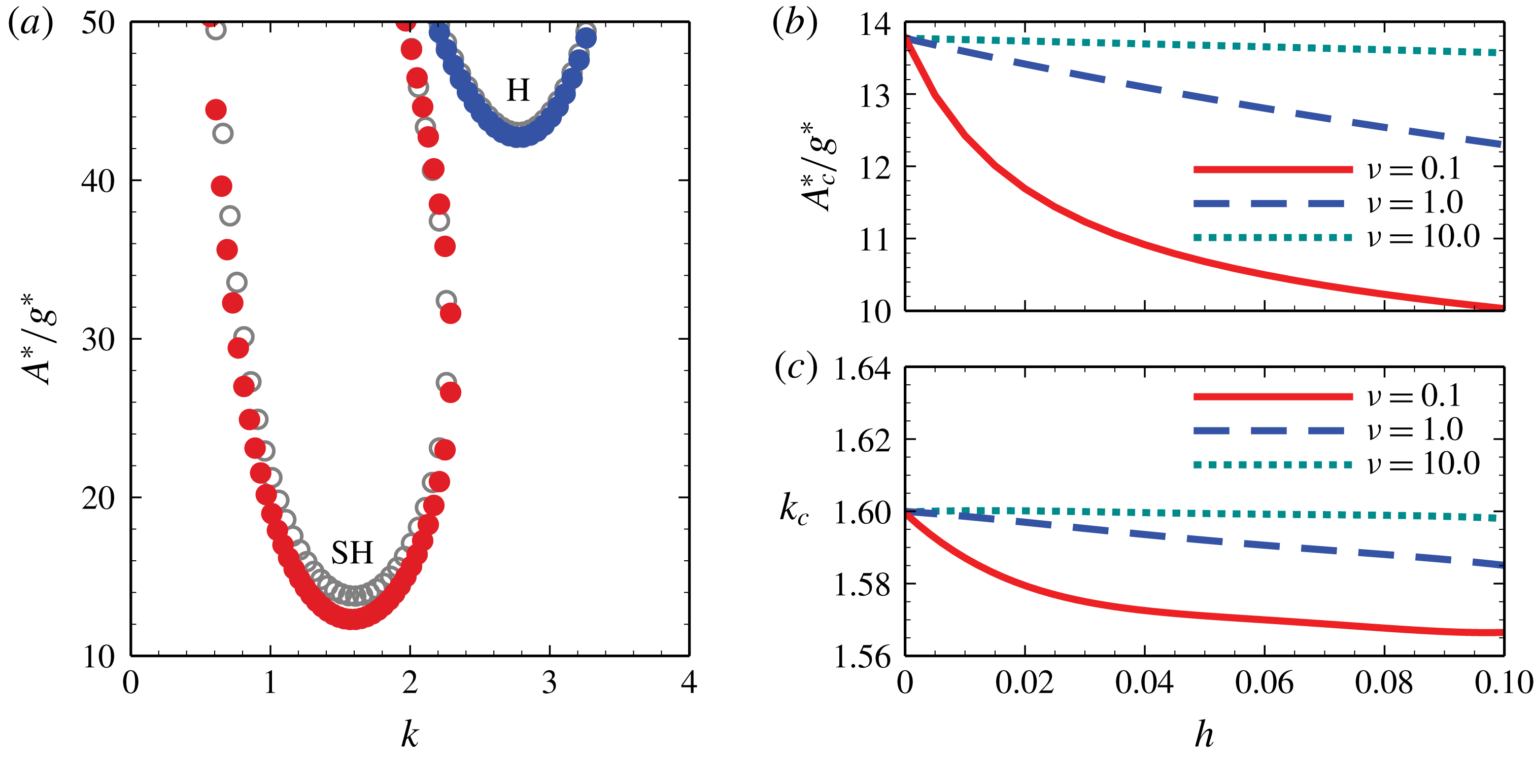
(a) Neutral stability curve for $\unicode[STIX]{x1D6FA}^{\ast }/2\unicode[STIX]{x03C0}=60~\text{Hz}$ and $\unicode[STIX]{x1D708}=1$ . The hollow circles represent the neutral stability curves corresponding to $h=0$ , which is the classical single-layer problem, while the solid circles represent the case of $h=0.1$ . The harmonic mode is denoted by H, while SH denotes the subharmonic mode. (b) The critical acceleration amplitude $A_{c}^{\ast }$ and (c) the corresponding critical wavenumber $k_{c}$ as functions of $h$ for different values of $\unicode[STIX]{x1D708}$ . The other parameters correspond to case (1) of table 1.

Table 1.

Parameters of liquid 2 for theoretical analysis ( $\unicode[STIX]{x1D70E}_{1}^{\ast }$ in case (2) shown in figure 8).

2.3.1 High oscillation frequency

As pointed out in previous work on single-layer systems (Kumar & Tuckerman Reference Kumar and Tuckerman1994; Kumar Reference Kumar1996), as long as the oscillation frequency is high enough, the most unstable mode is always subharmonic. As illustrated in figure 2(a) by the neutral stability curves for different values of $h$ , this situation is still maintained. As a consequence, only the subharmonic mode is investigated in the present subsection.

In figure 2(a), the effect due to the film at the bottom can be seen for $h=0.1$ . The neutral curve appears below the one for the classical single-layer case represented by $h=0$ . Hence, the thin film causes a lubrication effect in the thick layer by lowering the viscous drag, which makes it easier to destabilize the conjugated double-layer system than a single-layer one. Correspondingly, as shown in figure 2(b), the critical acceleration $A_{c}^{\ast }$ decreases when $h$ increases. Generally speaking, no matter how large the viscosity of the bottom film is, even if it is much higher than that of the top layer (e.g.  $\unicode[STIX]{x1D708}=10.0$ ), the lubrication effect always increases with $h$ . This results from the unavoidable flow at the liquid–liquid interface and inside the bottom film, which is induced by the flow in the top layer through the viscous shear at the interface. As the bottom film thickens, the viscous stresses are reduced, while in turn the lubrication effect is enhanced. The lubrication effect also increases as $\unicode[STIX]{x1D708}_{1}^{\ast }$ decreases. Compared with the classical result of $h=0$ , for $h=0.1$ , $A_{c}^{\ast }$ is reduced by only $1.5\,\%$ in the case of $\unicode[STIX]{x1D708}=10.0$ , but it is reduced by $27.2\,\%$ when $\unicode[STIX]{x1D708}=0.1$ . By contrast, the lubrication effect does not significantly influence the critical wavenumber of the instability. As shown in figure 2(c), the maximum variation of $k_{c}$ as $h$ increases is no more than $2.5\,\%$ .

Remarkably, all the curves in figure 2(b) have a positive second derivative with respect to $h$ . For $h=0.05$ , $A_{c}^{\ast }$ has already reduced by $22.4\,\%$ relative to its value at $h=0$ when $\unicode[STIX]{x1D708}=0.1$ . This indicates that the impact of lubrication is quite high when $h$ is small. As the film thickens, viscous stresses are reduced less efficiently, so that the lubrication effect increases less pronouncedly with increasing $h$ . Qualitatively, this mechanism should be active in any other case with different viscosities and viscosity ratios.

Figure 3.

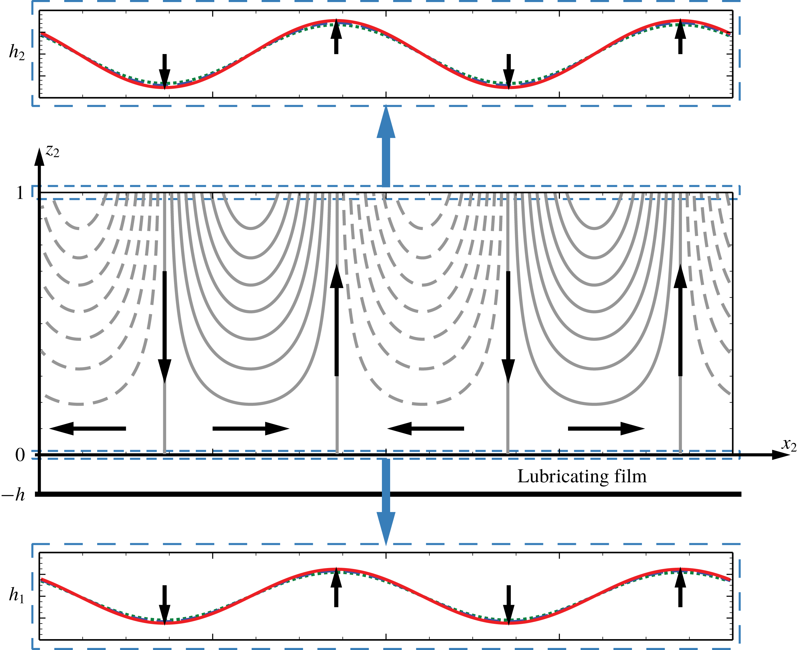
Flow structure of the critical state for $h=0.1$ , i.e. the lowest point on the curve composed by red solid dots in figure 2(a). The streamline patterns shown in the middle are taken at the initial moment, while the top surface and the liquid–liquid interface deformations are illustrated at three subsequent moments in order to show the evolution. The black arrows in each panel denote the flow direction and the direction of motion of the surface and the interface, respectively.

In figure 3, the flow structure in the linear regime of destabilization is illustrated. A time-periodic advection can be seen with arrows denoting the overall flow directions. Unlike Bénard–Marangoni convection (Nejati et al. Reference Nejati, Dietzel and Hardt2015), the velocity in the vertical direction does not vanish at the top free surface, since it is linked to the surface deformation. Hence, the streamlines in such Faraday systems are generally not closed. At the same time, this advection also triggers the deformation of the liquid–liquid interface through viscous shear. Owing to the large viscous and negligible inertial stresses in the thin film, the leading-order horizontal velocity profile inside the film is always a monotonic function of $z_{1}$ at a given location and time (see equation (A 20)). Caused by the velocity continuity, the deformation of the liquid–liquid interface is always synchronized with the top surface, i.e. both appear in the form of standing waves.

2.3.2 Low oscillation frequency

Figure 4.

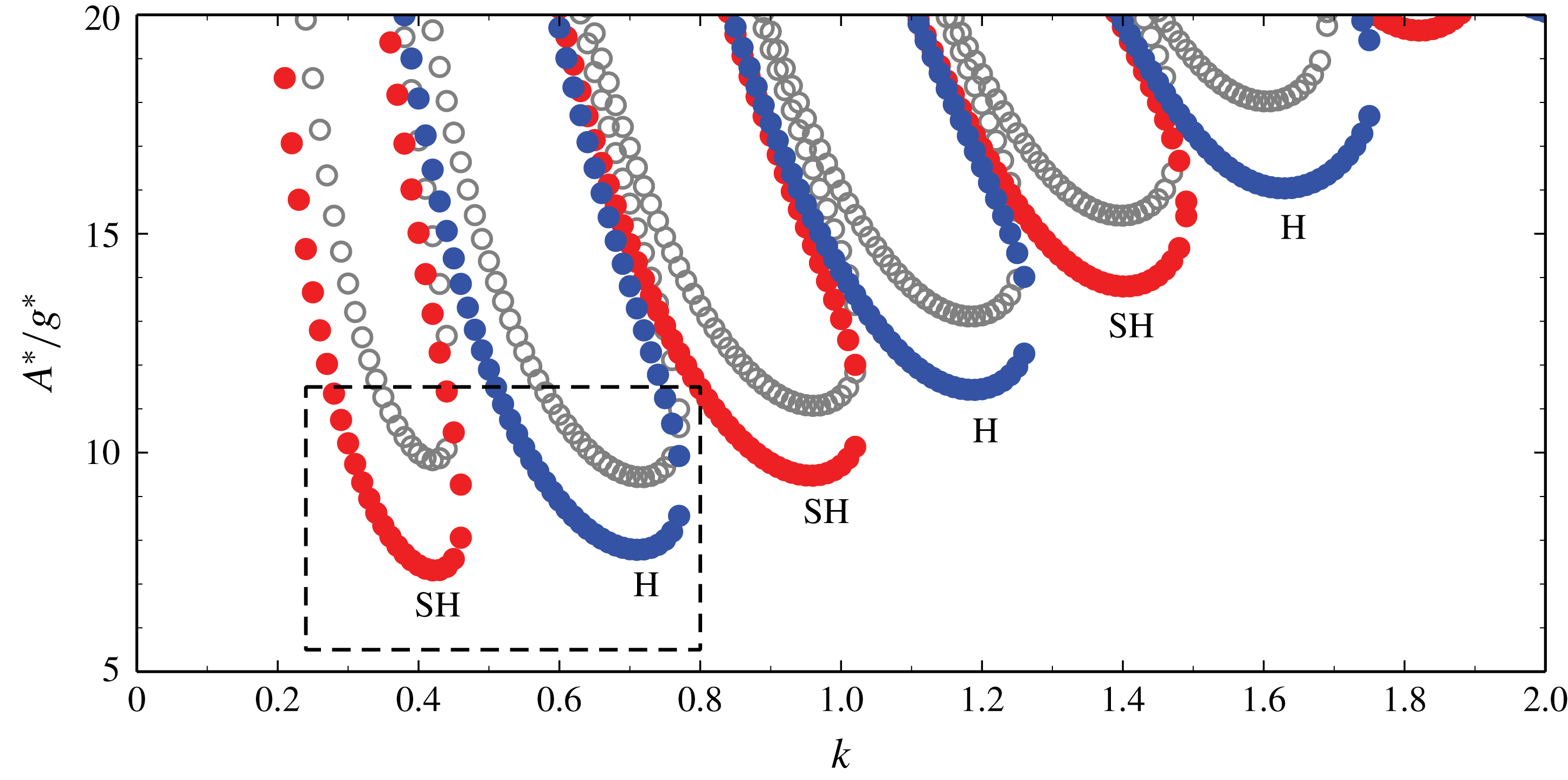
Neutral stability curves for $\unicode[STIX]{x1D6FA}^{\ast }/2\unicode[STIX]{x03C0}=8.5$  Hz and $\unicode[STIX]{x1D708}=1$ . The hollow circles indicate the neutral stability curves corresponding to $h=0$ , which represents the classical single-layered problem, while the solid dots correspond to $h=0.1$ . All other parameters are identical to case (1) of table 1. Harmonic modes are indicated by H, while SH denotes subharmonic modes.

Consistent with previous work (Kumar Reference Kumar1996), as the oscillation frequency is lowered, the wavenumbers of the unstable modes also decrease. This is illustrated in figure 4, where all of the tongue-like neutral stability curves become more slender with decreasing $k$ . Correspondingly, the horizontal length scale of the instability patterns increases in comparison to the case of larger frequencies. As shown by the two curves enclosed by the dashed frame, the critical acceleration decreases due to the presence of the film at the bottom, which is a behaviour equivalent to the high-frequency case (see figure 2).

Furthermore, at low frequencies, there appears a new effect due to the presence of the bottom film, namely the mode transition. Focusing on the region inside the dashed frame in figure 4, one sees that, if no bottom film is present ( $h=0$ ), the most unstable mode is harmonic. By contrast, for $h=0.1$ the most unstable mode is subharmonic. At high frequencies, it is known that no mode transition takes place (Kumar Reference Kumar1996). Thus, at a first glance the mode transition observed herein could be attributed to the low frequency. However, since this mode transition is only observed at low frequencies if a lubricating film is placed underneath the thicker layer, it might be related to the specific interplay between low driving frequencies and the lubricating film. To further illuminate the mode-transition phenomenon, we concentrate only on the two branches enclosed by the frame in figure 4. Transitions between other branches induced by further lowering the frequency (Kumar Reference Kumar1996) are beyond the scope of this work.

In previous work dealing with mode transition in single-layer systems (Kumar Reference Kumar1996), a boundary layer thickness was identified to be the relevant parameter affecting the mode transition. It was shown that, for decreasing boundary layer thickness, the subharmonic mode becomes more likely to be triggered than the harmonic one. Hence, to further explain the mode transition due to the lubrication effect, we need to define a corresponding characteristic thickness of an effective boundary layer in this two-layer system, $\unicode[STIX]{x1D6FF}_{e}^{\ast }$ , by employing the following train of thought:

1. (1) The characteristic length scale of the flow in the top layer is $h_{02}^{\ast }$ in each direction, and the corresponding characteristic velocity is $h_{02}^{\ast }\unicode[STIX]{x1D6FA}^{\ast }$ .

2. (2) The shear stress in the thick layer is characterized by $\unicode[STIX]{x1D70F}_{2}^{\ast }=\unicode[STIX]{x1D707}_{2}^{\ast }(h_{02}^{\ast }\unicode[STIX]{x1D6FA}^{\ast }-u_{1-2}^{\ast })/h_{02}^{\ast }$ , and that in the thin bottom film is given by $\unicode[STIX]{x1D70F}_{1}^{\ast }=\unicode[STIX]{x1D707}_{1}^{\ast }u_{1-2}^{\ast }/h_{01}^{\ast }$ , with $u_{1-2}^{\ast }$ denoting the horizontal component of velocity at the interface.

3. (3) The continuity of shear stress across the interface $\unicode[STIX]{x1D70F}_{1}^{\ast }=\unicode[STIX]{x1D70F}_{2}^{\ast }$ leads to an explicit expression for $u_{1-2}^{\ast }$ , while the continuity equation results in the vertical component of velocity at the interface $w_{1-2}^{\ast }$ .

4. (4) The inertial stress $\unicode[STIX]{x1D70C}_{2}^{\ast }u^{\ast }\unicode[STIX]{x2202}u^{\ast }/\unicode[STIX]{x2202}x^{\ast }=\unicode[STIX]{x1D70C}_{2}^{\ast }h_{02}^{\ast }\unicode[STIX]{x1D6FA}^{\ast }h_{02}^{\ast }\unicode[STIX]{x1D6FA}^{\ast }/h_{02}^{\ast }$ inside the boundary layer is balanced by the viscous stress, given by $\unicode[STIX]{x1D707}_{2}^{\ast }(\unicode[STIX]{x2202}^{2}u^{\ast }/\unicode[STIX]{x2202}{z^{\ast }}^{2}+\unicode[STIX]{x2202}^{2}w^{\ast }/\unicode[STIX]{x2202}{z^{\ast }}^{2})=\unicode[STIX]{x1D707}_{2}^{\ast }(h_{02}^{\ast }\unicode[STIX]{x1D6FA}^{\ast }-u_{1-2}^{\ast }+h_{02}^{\ast }\unicode[STIX]{x1D6FA}^{\ast }-w_{1-2}^{\ast })/{\unicode[STIX]{x1D6FF}_{e}^{\ast }}^{2}$ .

This results in an effective boundary layer thickness given by

(2.44) $$\begin{eqnarray}\displaystyle \unicode[STIX]{x1D6FF}_{e}^{\ast }=\sqrt{\frac{\unicode[STIX]{x1D708}_{2}^{\ast }}{\unicode[STIX]{x1D6FA}^{\ast }}\frac{\displaystyle 2+\frac{h}{\unicode[STIX]{x1D70C}\unicode[STIX]{x1D708}}(1-h)}{\displaystyle 1+\frac{h}{\unicode[STIX]{x1D70C}\unicode[STIX]{x1D708}}}}. & & \displaystyle\end{eqnarray}$$

Equation (2.44) is an extension of the classical result (Kumar Reference Kumar1996). Here, the lubrication effect is quantified by the dimensionless group $h/\unicode[STIX]{x1D70C}\unicode[STIX]{x1D708}$ , which influences $\unicode[STIX]{x1D6FF}_{e}^{\ast }$ significantly. Based on the results shown in figure 4, extending the previous train of thought and assuming that we are given $\unicode[STIX]{x1D708}_{2}^{\ast }$ and $\unicode[STIX]{x1D6FA}^{\ast }$ , we find that, if the lubrication effect is strengthened either by increasing $h$ or reducing $\unicode[STIX]{x1D708}$ , $\unicode[STIX]{x1D6FF}_{e}^{\ast }$ decreases, and the subharmonic mode can be excited more easily. Conversely, when the lubrication effect is reduced, the effective boundary layer thickness increases, and the harmonic mode becomes the most unstable one. Furthermore, as $h$ vanishes, $\unicode[STIX]{x1D6FF}_{e}^{\ast }$ asymptotes to the classical result for the single-layer system, and so do the corresponding neutral stability curves.

Figure 5.

Critical acceleration $A_{c}^{\ast }$ corresponding to the two lowest harmonic and subharmonic modes as a function of the thickness ratio $h$ . The parameters of case (1) in table 1 were considered, with $\unicode[STIX]{x1D708}=1$ and $\unicode[STIX]{x1D6FA}^{\ast }/2\unicode[STIX]{x03C0}=8.5~\text{Hz}$ , respectively.

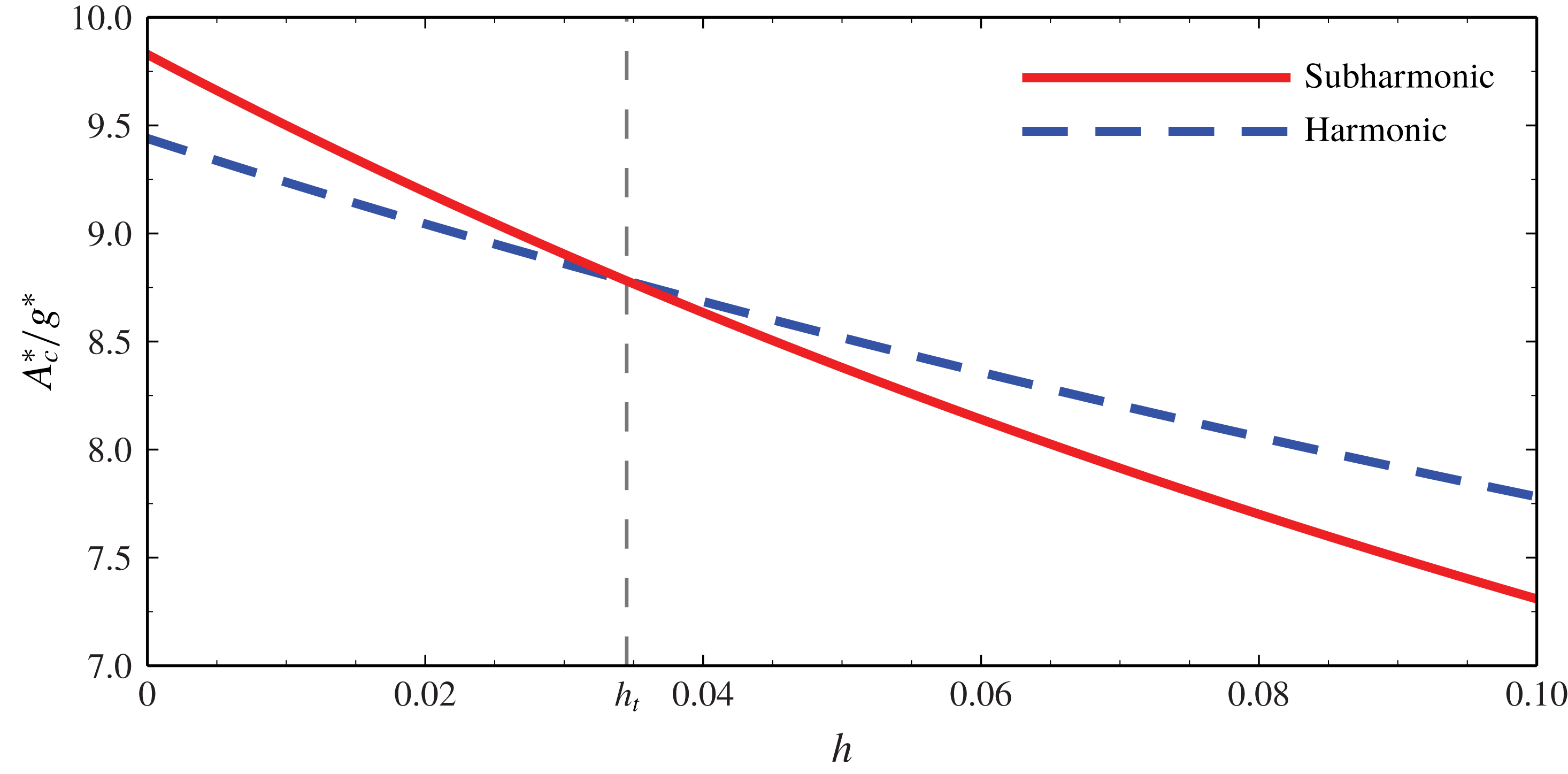
The critical accelerations $A_{c}^{\ast }$ of both modes should behave as monotonically decreasing functions of $h$ , provided $\unicode[STIX]{x1D708}$ is fixed. However, as shown in figure 5, the slopes are quite different. The harmonic mode is more unstable when $h$ is small, but the critical acceleration for this mode decreases more slowly than that of the subharmonic mode as $h$ increases to $0.1$ . As a consequence, a mode transition occurs at $h_{t}\approx 0.0345$ . By contrast, the critical wavenumbers $k_{c}$ of the two modes are quite insensitive to the variation of $h$ (not shown in the paper). For the subharmonic mode, $k_{c}$ maintains around $0.423$ , while for the harmonic mode it is around $0.714$ . Hence, the spatial periodicities of the flow structures are not significantly different from those of the single-layer system.

Figure 6.

Critical acceleration corresponding to the two lowest harmonic and subharmonic modes as a function of $h/\unicode[STIX]{x1D708}$ . The parametric values of case (1) of table 1 were used with $\unicode[STIX]{x1D6FA}^{\ast }/2\unicode[STIX]{x03C0}=6.0~\text{Hz}$ .

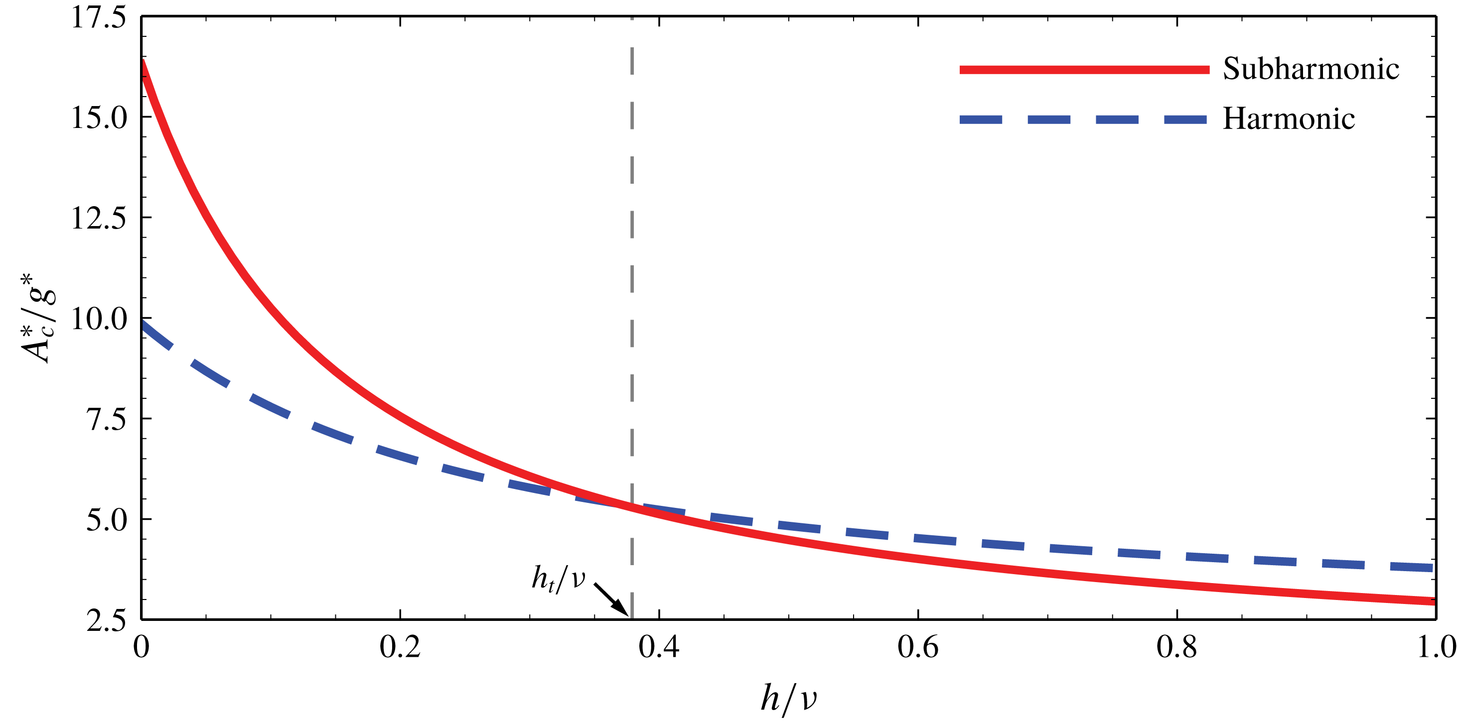
Since $\unicode[STIX]{x1D6FF}_{e}^{\ast }$ is mainly determined by $h/\unicode[STIX]{x1D708}$ (2.44) provided other parameters, such as $\unicode[STIX]{x1D708}_{2}^{\ast }$ , $\unicode[STIX]{x1D6FA}^{\ast }$ and $\unicode[STIX]{x1D70C}$ are fixed, the critical accelerations of each mode should be located along a uniform curve in terms of $h/\unicode[STIX]{x1D708}$ , as seen from figure 6. In order to further clarify the correlation between the transition threshold and the lubrication effect, several cases with different frequencies were calculated, and the results are shown in figure 7 and table 2, respectively.

Figure 7.

Critical thickness ratio of the mode transition $h_{t}$ as a function of the viscosity ratio $\unicode[STIX]{x1D708}$ for different values of $\unicode[STIX]{x1D6FA}^{\ast }/2\unicode[STIX]{x03C0}$ . From left to right, the curves correspond to: 5.0 Hz (▵), 6.0 Hz (▹), 7.0 Hz (◃), 7.8 Hz (

), 8.0 Hz (○), 8.5 Hz (▫), 8.7 Hz (♢) and 8.9 Hz ( $\times$ ). The parametric values of case (1) of table 1 were considered, and the curve slopes are shown in table 2 in detail.

Table 2.

Average values of $h_{t}/\unicode[STIX]{x1D708}$ , their variances and corresponding effective Reynolds number $Re_{e}$ at the threshold for different frequencies $\unicode[STIX]{x1D6FA}^{\ast }/2\unicode[STIX]{x03C0}$ corresponding to figure 7.

In figure 7, we see that $h_{t}$ is approximately a linear function of $\unicode[STIX]{x1D708}$ . The statistics of the average ratio $h_{t}/\unicode[STIX]{x1D708}$ , as shown in table 2, confirms this linearity with sufficiently small variance (no more than 0.9 %). Accordingly, it is reasonable to consider that, for a given frequency, the mode transition can be characterized by a fixed value of $h_{t}/\unicode[STIX]{x1D708}$ . Referring to the definition of $\unicode[STIX]{x1D6FF}_{e}^{\ast }$ we define an effective Reynolds number $Re_{e}$ as follows:

(2.45) $$\begin{eqnarray}\displaystyle Re_{e}=\frac{\displaystyle \unicode[STIX]{x1D70C}_{2}^{\ast }u^{\ast }\frac{\unicode[STIX]{x2202}u^{\ast }}{\unicode[STIX]{x2202}x^{\ast }}}{\displaystyle \unicode[STIX]{x1D707}_{2}^{\ast }\left(\frac{\unicode[STIX]{x2202}^{2}u^{\ast }}{\unicode[STIX]{x2202}{z^{\ast }}^{2}}+\frac{\unicode[STIX]{x2202}^{2}w^{\ast }}{\unicode[STIX]{x2202}{z^{\ast }}^{2}}\right)}=\frac{\displaystyle \unicode[STIX]{x1D70C}_{2}^{\ast }h_{02}^{\ast }\unicode[STIX]{x1D6FA}^{\ast }\frac{h_{02}^{\ast }\unicode[STIX]{x1D6FA}^{\ast }}{h_{02}^{\ast }}}{\displaystyle \unicode[STIX]{x1D707}_{2}^{\ast }\frac{h_{02}^{\ast }\unicode[STIX]{x1D6FA}^{\ast }-u_{1-2}^{\ast }+h_{02}^{\ast }\unicode[STIX]{x1D6FA}^{\ast }-w_{1-2}^{\ast }}{{h_{02}^{\ast }}^{2}}}=Re_{2}\frac{\displaystyle 1+\frac{h}{\unicode[STIX]{x1D70C}\unicode[STIX]{x1D708}}}{\displaystyle 2+\frac{h}{\unicode[STIX]{x1D70C}\unicode[STIX]{x1D708}}(1-h)}. & & \displaystyle \nonumber\\ \displaystyle & & \displaystyle\end{eqnarray}$$

Therefore, once $\unicode[STIX]{x1D6FA}^{\ast }$ , $h_{02}^{\ast }$ , $\unicode[STIX]{x1D708}_{2}^{\ast }$ and $\unicode[STIX]{x1D70C}$ are fixed, referring to table 2, the mode transition happens at a given value of $Re_{e}$ with sufficient precision owing to the small value of $h$ . The extreme case is represented by $\unicode[STIX]{x1D6FA}^{\ast }/2\unicode[STIX]{x03C0}=8.9$  Hz, in which the mode transition occurs at $h=h_{t}\rightarrow 0$ . In this case, no matter how much $\unicode[STIX]{x1D708}$ is increased, $h_{t}\equiv 0$ and $Re_{e}\equiv Re_{2}/2$ .

2.3.3 Single-layer system with Navier-slip boundary condition

One would expect that the main effect of a low-viscosity bottom film is to reduce the shear stress inside the top layer. This mechanism is quite similar to the classical Navier-slip boundary condition in a single-layer system, which is characterized via an empirical parameter called the effective slip length $\unicode[STIX]{x1D6FD}^{\ast }$ . If we ignore the interface deformation by setting $h_{1}^{\prime }=0$ and $\unicode[STIX]{x1D735}_{2}w_{2}^{\prime }=0$ , equation (2.32) becomes

(2.46) $$\begin{eqnarray}\displaystyle \frac{\unicode[STIX]{x2202}w_{2}^{\prime }}{\unicode[STIX]{x2202}z_{2}}=\frac{h}{\unicode[STIX]{x1D70C}\unicode[STIX]{x1D708}}\frac{\unicode[STIX]{x2202}^{2}w_{2}^{\prime }}{\unicode[STIX]{x2202}z_{2}^{2}}, & & \displaystyle\end{eqnarray}$$

which is mathematically consistent with the Navier-slip condition (after non-dimensionalization employing the same scales) since $h/\unicode[STIX]{x1D70C}\unicode[STIX]{x1D708}$ is equivalent to $\unicode[STIX]{x1D6FD}^{\ast }/h_{20}^{\ast }$ . In other words, under these assumptions, the present two-layer system is a generalization of the classical one with a Navier-slip condition applied to the bottom boundary of the layer. However, in typical systems, $\unicode[STIX]{x1D6FD}^{\ast }$ attains values only between a few nanometres and one micrometre (Shu, Teo & Chan Reference Shu, Teo and Chan2017). The present system offers a much larger range of the equivalent slip length. For example, as shown later in the section of experimental results, $h/\unicode[STIX]{x1D70C}\unicode[STIX]{x1D708}$ can reach values up to $0.14$ , i.e. the equivalent slip length achieves $0.14h_{20}^{\ast }$ . In fact, as discussed later, this maximum is mainly limited by the onset of the Rayleigh–Taylor instability. If the lubricating film used had a larger density, this maximum would be even higher.

Figure 8.

Critical acceleration in terms of the depth ratio $h$ for different values of the interfacial tension $\unicode[STIX]{x1D70E}_{1}^{\ast }$ . The physical properties of the liquid in the upper layer correspond to case (2) of table 1 with $\unicode[STIX]{x1D6FA}^{\ast }/2\unicode[STIX]{x03C0}=60~\text{Hz}$ and $\unicode[STIX]{x1D708}=1.0$ .

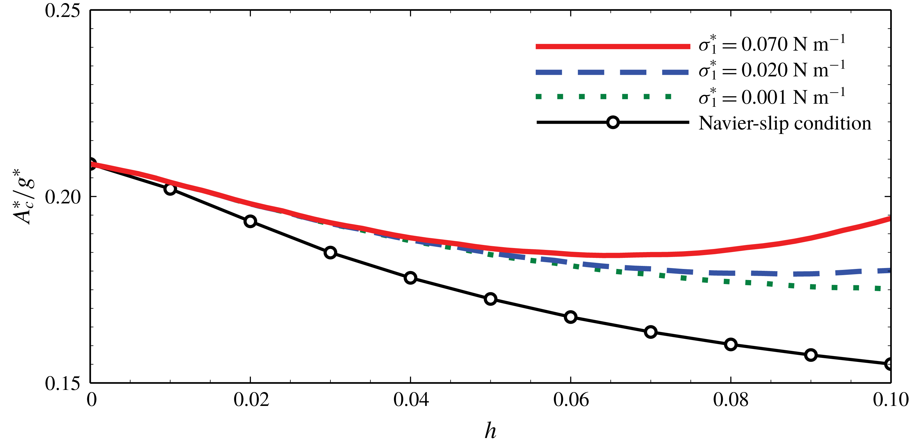
Furthermore, the interface deformation of the two-layer system introduces a new aspect not captured by a Navier-slip model. How far the analogy to a single-layer system carries is documented in figure 8, which shows the critical acceleration for different values of interfacial tension $\unicode[STIX]{x1D70E}_{1}^{\ast }$ . The single-layer and the two-layer models predict virtually indistinguishable critical wavenumbers $k_{c}\approx 1.530$ with maximum deviation around $0.4\,\%$ (not shown), but for the critical acceleration $A_{c}^{\ast }$ some significant deviations become apparent and more prominent as $h$ increases. These deviations are mainly influenced by two factors: the interfacial capillarity and the magnitude of the bulk force $\boldsymbol{f}^{\ast }$ . Based on (2.31), capillarity is proportional to $-\tilde{S}_{1}\tilde{\unicode[STIX]{x1D6FB}}_{1}^{4}h_{1}^{\prime }$ or, within the framework of the normal-mode analysis, proportional to $-\tilde{S}_{1}k^{4}h_{1}^{\prime }$ , where $\tilde{S}_{1}$ is the non-dimensional form of the interfacial tension $\unicode[STIX]{x1D70E}_{1}^{\ast }$ . Hence, capillarity always dampens the temporal increase of the deformation $\unicode[STIX]{x2202}h_{1}^{\prime }/\unicode[STIX]{x2202}\tilde{t}_{1}$ . For vanishing $\unicode[STIX]{x1D70E}_{1}^{\ast }$ one may expect that the curve of $A_{c}^{\ast }/g^{\ast }$ as a function of $h$ as shown in figure 8 becomes identical to the curve representing the Navier-slip boundary. This is not the case, since any flow in thin films governed by the lubrication approximation always goes along with an interfacial deformation, which is pronounced for small interfacial tension and proportional to $\tilde{\unicode[STIX]{x1D6FB}}_{1}^{2}h_{1}^{\prime }$ (equivalent to $-k^{2}h_{1}^{\prime }$ ). This further dampens $\unicode[STIX]{x2202}h_{1}^{\prime }/\unicode[STIX]{x2202}\tilde{t}_{1}$ and stabilizes the system. Therefore, generally speaking, the single-layer system with Navier-slip condition would only be equivalent to the two-layer system if the deformation of the interface of the two-layer system were completely negligible. For a non-vanishing deformation, even a vanishing interfacial tension will always give a mismatch between the single- and double-layer models.

Figure 9.

Schematic configuration of experimental set-up, including the shadowgraphy system and the cross-section of the container.

Note that the results presented in figure 8 correspond to case (2) of table 1. Case (2) implies sufficiently large values of $\tilde{S}_{1}$ and $G_{1}$ of the order of $O(10^{2})$ for $h=0.1$ . By contrast, for case (1) these two values are only of the order of $O(1)$ or even smaller. As a consequence, the effect linked to an interfacial deformation becomes more difficult to observe.

3.1 Set-up

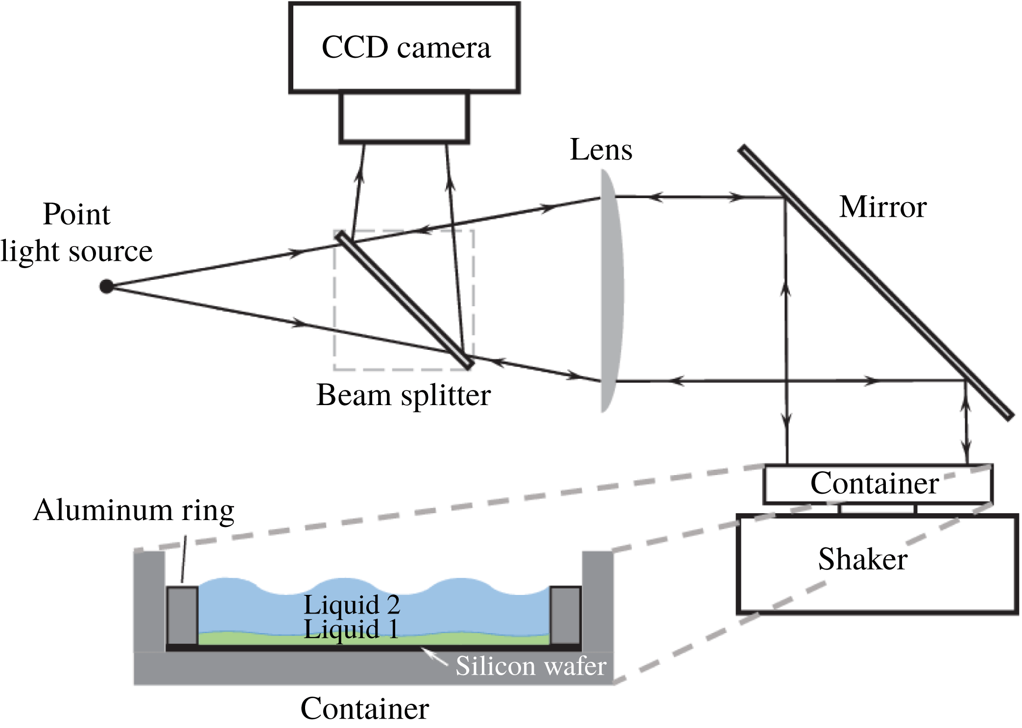
The above theoretical predictions are validated through experimental investigations. As illustrated schematically in figure 9, the visualization of surface and interface deformations is accomplished by the shadowgraphy technique. A point light source is placed at the focal point of a lens (Thorlabs, focal length $250$  mm, diameter $50.8$  mm). A parallel light beam is generated in the horizontal direction behind the lens. After reflection at a mirror tilted at $45^{\circ }$ , the parallel light is directed downwards, and illuminates an aluminium container, whose bottom wall is mounted horizontally on top of a shaker (Brüel & Kjaer, Type 4809). The shaker works within a closed loop, including two accelerometers (Brüel & Kjaer, Miniatur Hex IEPE), a power amplifier (Brüel & Kjaer, Type 2706), a control device (Brüel & Kjaer, Dactron Comet USB2.0) and a personal computer. A silicon wafer (diameter $101.6$  mm) is placed inside the container, so that the incident light is reflected back. An aluminium ring with height $1$  mm and inner diameter $90$  mm is pressed onto the silicon wafer by tightening screws. Hence, a volume of small height-to-width ratio is created into which two immiscible liquids are injected. Because a beam splitter is placed between the light source and the lens, the reflected beam can finally be redirected into a charge-coupled device (CCD) camera (Nikon DS-Qi1Mc, resolution $1280\times 1024$ ). Any deformation of either the liquid surface or the liquid–liquid interface induces a redistribution of the beam intensity, so that the flow inside the container can be indirectly recorded and analysed.

In the experiments, the bottom lubricating film (liquid 1) is a silicone oil (3 cSt, Elbesil), and the upper thicker layer is a perfluorinated hydrocarbon (FC-70, Sigma-Aldrich), which are the same as used in the work of Nejati et al. (Reference Nejati, Dietzel and Hardt2015). Since FC-70 has a small surface tension and a small contact angle with aluminium, which in addition is only weakly affected by contaminants, it has been proven to be a practicable choice for such double-layer experiments. The major reason that silicone oil is chosen as the bottom lubricating layer is its almost perfect wetting of the silicon wafer, while there is a broad range of viscosities available. In the present case, a low viscosity, sufficiently lower than that of FC-70, is helpful to enhance the lubrication effects. Good wettability helps to generate a stable thin film over the wafer without film rupture occurring.

It is noted that the higher density of FC-70 compared to silicone oil leads to the Rayleigh–Taylor instability (RTI) of the interface. However, the instability can be suppressed within the time span of the experiments by choosing sufficiently thin oil films. The limitation of layer thicknesses is estimated by requiring the viscous diffusion time scale of the RTI, given by $\unicode[STIX]{x1D70F}_{vis}^{\ast }={h_{01}^{\ast }}^{2}/\unicode[STIX]{x1D708}_{1}^{\ast }$ , to be much shorter than its dynamic time scale, given by $\unicode[STIX]{x1D70F}_{dyn}^{\ast }=\sqrt[4]{27(\unicode[STIX]{x1D70C}_{2}^{\ast }+\unicode[STIX]{x1D70C}_{1}^{\ast })^{2}\unicode[STIX]{x1D70E}_{1}^{\ast }/[4(\unicode[STIX]{x1D70C}_{2}^{\ast }-\unicode[STIX]{x1D70C}_{1}^{\ast })^{3}g^{\ast 3}]}$ (the inverse of the fastest temporal growth rate of RTI (Piriz et al. Reference Piriz, Cortázar, López Cela and Tahir2006)). Owing to the necessity of pinning the top free surface at the edge of the lateral walls (Douady & Fauve Reference Douady and Fauve1988; Douady Reference Douady1990; Edwards & Fauve Reference Edwards and Fauve1993; Gluckman et al. Reference Gluckman, Marcq, Bridger and Gollub1993), on the one hand, and fabrication constraints, on the other, the height of the aluminium ring, i.e.  $h_{01}^{\ast }+h_{02}^{\ast }$ , is fixed to be $1$  mm. Accordingly, considering all constraints, $h_{01}^{\ast }\ll 0.263~\text{mm}$ should be guaranteed, which corresponds to $h\ll 0.357$ . As shown later in figure 11, $h<0.02$ for all experiments conducted, i.e. sufficiently less than this upper limit. In addition, as discussed in previous works (Troyon & Gruber Reference Troyon and Gruber1971; Hoffmann & Wolf Reference Hoffmann and Wolf1974; Sterman-Cohen, Bestehorn & Oron Reference Sterman-Cohen, Bestehorn and Oron2017), since vibration is the driving force of the Faraday instability, it can stabilize the RTI by restraining its development to a saturated state. Therefore, the present system should generally have a weaker RTI in comparison to those without vibration (Nejati et al. Reference Nejati, Dietzel and Hardt2015).

Figure 10.

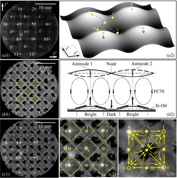
Typical experimental observations of the cellular structure of the conjugated liquid layers, with $h=8.89\times 10^{-4}$ , $A^{\ast }/g^{\ast }=2.400$ and $\unicode[STIX]{x1D6FA}^{\ast }/2\unicode[STIX]{x03C0}=30~\text{Hz}$ . (a1) Snapshot of top surface during vibration, with (a2) showing a local schematic configuration. (b1) Snapshot right after the vibration has stopped, with (b2) showing schematically the advection inside the layers. (c1) Superposition of (a1) and (b1), with (c2) being a local magnification, and (c3) a further magnification of (c2) with illustrated flow structure. The open circles indicate the accumulation points under the antinodes of the standing wave, the crosses the sweeping points, and the square illustrates the location where both accumulation and sweeping occur. The large and small bright regions in (b1) and (c1) are enclosed by solid and dashed boundaries, respectively.

Figure 11.

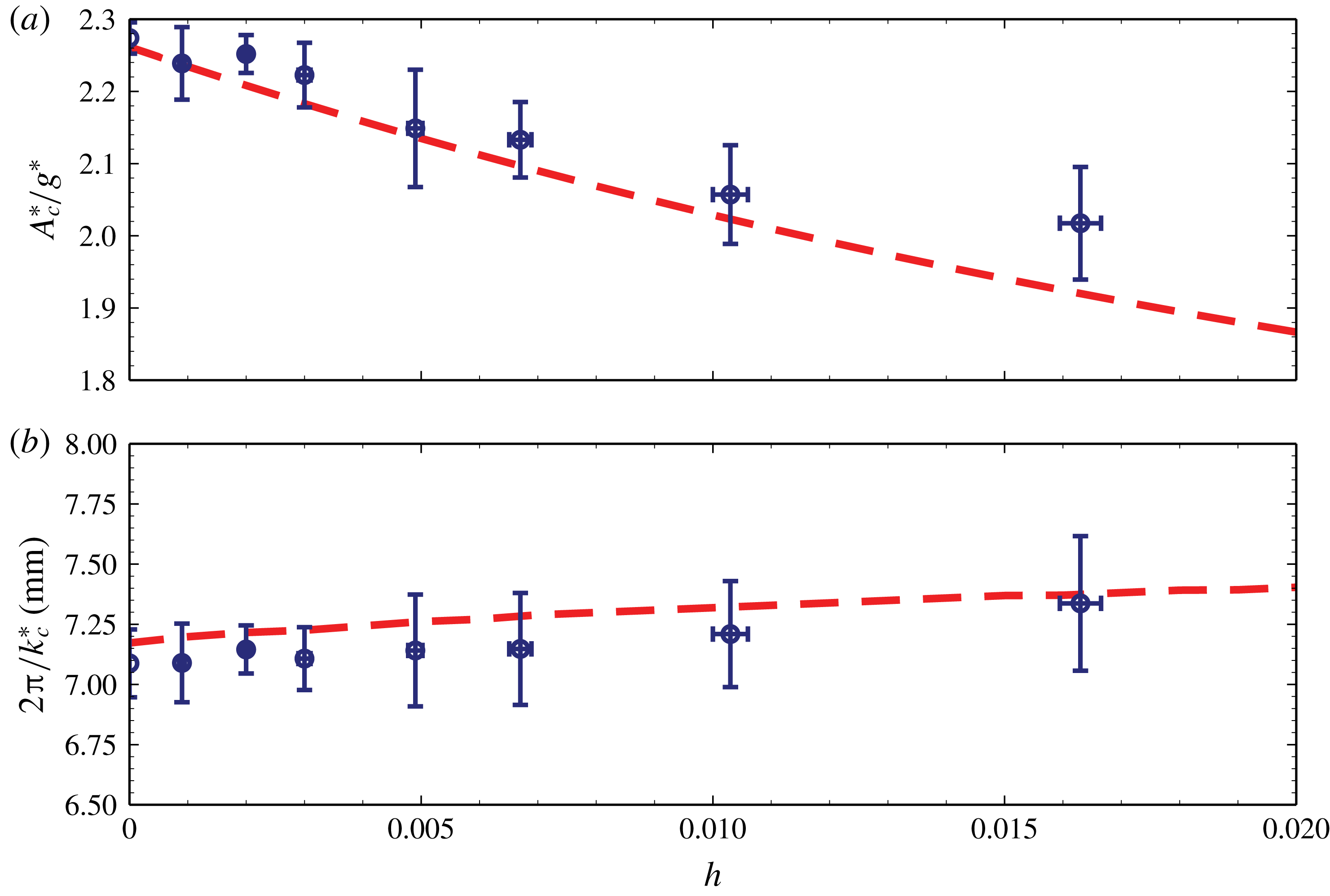
Theoretically predicted variations of (a) the critical acceleration $A_{c}^{\ast }$ and (b) the critical wavelength with $h$ (dashed lines) for $\unicode[STIX]{x1D6FA}^{\ast }/2\unicode[STIX]{x03C0}=30~\text{Hz}$ . The corresponding experimental results are shown as symbols with error bars.

3.2 Results and discussion

Consistent with the previous investigations (Gluckman et al. Reference Gluckman, Marcq, Bridger and Gollub1993), only when the driving acceleration sufficiently exceeds the threshold of destabilization can Faraday waves with clear structures be observed experimentally. For instance, the results shown in figure 10 have been obtained for a driving acceleration of $A^{\ast }=2.400g^{\ast }>A_{c}^{\ast }=2.236g^{\ast }$ . From the shadowgraphy technique it is known that every labelled bright spot in figure 10(a1) corresponds to an antinode of the standing (Faraday) wave, which is shown schematically in figure 10(a2). One can sort the spots into two different groups, labelled either by numbers or letters, where all members of one group share a similar instantaneous brightness. This instantaneous brightness differs from one group to the next, while the group brightness varies alternately with time.

As pointed out previously (Nejati et al. Reference Nejati, Dietzel and Hardt2015), the brighter spots shown in figure 10(a1) are a consequence of a local convex deformation of the surface, whereas the darker spots are caused by local concavity. Hence, the group of spots labelled by numbers represent peaks of the Faraday waves, while the group of spots labelled by letters correspond to valleys (see figure 10 a1,a2). Accordingly, the distance between two adjacent spots in the same group (either labelled by arabic numbers or by letters) represents one spatial period. The wave pattern shown in figure 10(a1,a2) can be roughly characterized by $h_{1,2}^{\ast }(x^{\ast },y^{\ast },t^{\ast })\sim \sin (0.5\unicode[STIX]{x1D6FA}^{\ast }t^{\ast })[\sin (k^{\ast }x^{\ast })+\sin (k^{\ast }y^{\ast })]$ , where $k^{\ast }$ denotes the dimensional wavenumber, and $x^{\ast }$ and $y^{\ast }$ , respectively, denote the axes parallel to the connection of spots. For the subsequent discussion of the flow pattern, it is noted that, given the square symmetry of the Faraday waves, apart from the nodes of the oscillating liquid surface, there are two additional categories of points. The points labelled by arabic numbers or letters are local maxima or minima, i.e. antinodes, while those labelled by roman numbers are saddle points of the deformed surface; see figure 10(a2). In other words, points I and II are simultaneously both peaks and valleys for two standing waves that are perpendicular to each other. As discussed below, the nodes, the antinodes and the saddle points translate into distinct deformation modes of the liquid–liquid interface.

Almost immediately after the shaker is turned off, the flow inside the upper thick layer is damped out quickly due to the high viscosity of FC-70, and the upper free surface becomes flat. However, the deformed liquid–liquid interface takes much more time to smoothen, because it needs to overcome the viscous dissipation not only from the lubricating oil film itself, but also from the FC-70 layer. This provides sufficient time to observe the remaining interface deformation through the grey-level distribution, as illustrated in figure 10(b1). The dark areas represent those regions where the bottom film is thinned, while the bright areas are located where the film is thickened (Nejati et al. Reference Nejati, Dietzel and Hardt2015). Although the maxima and minima of the top surface are reversed after one half-cycle, the interface deformation does not follow this temporal periodicity, but a steady-state configuration builds up after a number of periods. Following the discussion of Douady (Reference Douady1990) and as illustrated in figure 10(b2), it appears only after the flow in the upper layer has reached the nonlinear regime. In other words, if the flow were linear, no measurable deformation at the liquid–liquid interface should emerge since the shear stresses acting on the interface would be completely reversed in the next half-cycle. The nonlinearity ensures that these time-integrated shear stresses are non-vanishing, so the interface deformation is an indirect proof of the nonlinear flow structure. By superimposing figure 10(a1) and (a2) to obtain figure 10(c1), one sees that the deformation is strongly correlated to that of the top surface.

As indicated in figure 10(c1,c2) by solid or dashed lines, there are three distinct types of areas. Beneath antinodes of the liquid surface one finds larger grey areas, indicating a strong accumulation of oil caused by a corresponding flow in the FC-70 layer. The dark areas, indicating oil removal by a sweeping flow, are beneath nodes. Finally, smaller grey areas, indicating weaker oil accumulation, are located beneath the saddle points of the liquid surface. Hence, nodes of the oscillating liquid surface lead to oil removal in the thin film, while antinodes lead to strong oil accumulation. The saddle points represent local minima or maxima, depending on the direction along the surface. Therefore, their effect is similar to that of the antinodes, but the oil accumulation is somewhat weaker.

As shown in figure 10(c3), the superposition of accumulating and sweeping flow inside the upper layer is qualitatively compatible with the flow structure found by Douady (Reference Douady1990) and Périnet et al. (Reference Périnet, Gutiérrez, Urra, Mujica and Cordillo2017) through particle-based imaging techniques. The velocity vectors point towards accumulation points (indicated by open circles) and away from sweeping points (indicated by crosses). The filled square is a hyperbolic point, i.e. fluid is accumulated in the I–II direction but swept in the 4–e direction. Because the surface deformation in the I–II direction is weaker, the strength of accumulation is weaker, so it leads to a net sweeping around the filled square point. Note that since the denoted points coincide with locations where the flow is in the vertical direction only, they mark also the borders of advection cells.

A quantitative comparison between experimental observations and theoretical predictions is made through the critical wavelength and the critical acceleration for various layer thickness ratios. The former is measured as the distance between adjacent spots of identical brightness, as described above. While ramping up the acceleration by changing the vibration amplitude at fixed frequency of the shaker, the critical value of the acceleration is taken as the threshold state when the flow structure becomes visible for the first time. This is the moment when the brightness distribution under the camera starts to become inhomogeneous. The theoretical predictions are obtained from the model of § 2 by using the physical properties of the fluids from the experiments. No empirical parameter for data fitting is needed. As shown in figure 11, excellent agreement between the experimental and theoretical findings is observed. Owing to the unavoidable RTI, which is augmented as $h$ increases, it is anticipated that the maximum error of $A_{c}^{\ast }\approx 5\,\%$ belongs to the case $h=16.266\times 10^{-3}$ . Our experimental results underline the validity and accuracy of our theoretical predictions.