1. The Cases

Let us start with the case that has been most discussed in this literature, a case of heterozygote superiority. Let us suppose that there is a single genetic locus with two alleles, A and a. Thus there are three genotypes, AA, Aa, and aa.. By definition the heterozygote Aa is superior in fitness to the two homozygotes. In general the fitness of the two homozygotes need not be equal, but for simplicity we will assume that they are since nothing hinges on that assumption. The standard genotypic model normalizes the fitness of Aa at 1 and assigns the fitness of $1-s$ to the two homozygotes (where $1\geq s> 0$ ). Although the value of $s=1$ is a mathematical, and biological, possibility, for our purposes we cannot focus on that value since it is what Brandon (Reference Brandon2005) has termed a value of maximal fitness difference. Fitness values are at the point of maximal fitness difference when some fitness values equal 1 and some equal 0 and there are no intermediary fitness values. Drift is impossible at a maximal fitness differential point. Since we are going to be interested in the interplay of drift and selection, we will need to give s some intermediary value. For now let us assume $s=0.5$ . This model predicts a stable equilibrium that will be reached in a number of generations (depending on the initial starting point and population size). At this equilibrium the frequencies of the two alleles are both 50%.

The genic selectionist looks at the same situation and describes it differently. The two alleles, A and a, are in competition with each other. Their fitness depends on their allelic environment. A has a low fitness when it finds itself paired with another copy of itself but has a high fitness when paired with a. Conversely for a. Selection in this case is frequency-dependent. For example, if a starts at a low frequency, then it will almost exclusively find itself in the favorable allelic environment of being paired with an A. Thus a would be assigned a high fitness value and A a low value. This difference in fitness between a and A persists for however many generations it takes to reach equilibrium, but the fitness difference decreases as equilibrium is approached. After the equilibrium is reached, both have equal fitness.

The genotypic model says that selection among the three genotypes occurs each generation, but that because of Mendelian inheritance the $Aa\times Aa$ matings produce offspring of the genotypes AA, Aa, and aa in the ratio of 1:2:1. Thus the stable equilibrium is the result of selection and Mendelism (or, more generally, the genetic and mating systems). But the genic selectionist must say that once the equilibrium is reached, selection no longer occurs because the fitnesses of the two alleles are the same. As we will see shortly, s, the selection differential, is a crucial parameter in models of selection and drift. The genotypic model has $s=0.5$ in our example. This is true at equilibrium and at every other point in gene frequency space; that is, fitness is frequency-independent. However, for the genic selectionist, selection is frequency-dependent. At equilibrium all alleles have the same fitness, so $s^{*}=0$ . (We will use s* as the genic analogue of the genotypic selection coefficient, s. We will show how it relates to s shortly.)

But when there are two alleles at a locus and they are selectively neutral, evolutionary genetics gives a very clear prediction. The frequencies of the two alleles will drift (i.e., move randomly in allele state space). If that selective neutrality were frequency-independent, then one of the two alleles would drift to fixation.Footnote ² It is important to note that population size is irrelevant to the qualitative prediction just described.Footnote ³ However, for the genic selectionist the allelic fitnesses are not frequency-independent, and so as the population drifts away from the equilibrium point, genic selection will increase in magnitude and push the population back toward equilibrium. Thus both the genic and genotypic models predict the same equilibrium point, but, as we will see, they predict different trajectories toward that point. The genotypic model predicts a stable equilibrium. This prediction is based on selection actively maintaining the equilibrium. The genic model is forced to say that no selection occurs at equilibrium. But if no selection is occurring, then the population will drift (see Brandon Reference Brandon2006). Once drift moves the population sufficiently, selection will tend to move it back toward equilibrium.

It is important to note that these two models make factually different predictions that are detectably different even over a few generations. However, the predictions are probabilistic. Thus we should not expect the two models to predict actual outcomes that are mutually exclusive. To illustrate, suppose that we have one particular coin and have two hypotheses concerning its chances for producing heads when tossed. Hypothesis 1 says that the $\mathrm{Pr}\,(H) =0.5$ and hypothesis 2 is that $\mathrm{Pr}\,(H) =0.75$ . Suppose now that we toss the coin 10 times. The possible outcomes, the number of heads, range from zero to 10. Each outcome is logically compatible with both hypotheses. But the important point is that the hypotheses make different predictions, and given enough tosses, we can easily distinguish between the two hypotheses (using, e.g., likelihood methods [Edwards Reference Edwards1992]). In principle our case is not different. What we will show is that for a range of parameter values, the two models make different (probabilistic) predictions. In contrast to the coin toss case, gathering the appropriate data from natural populations is not at all easy.Footnote ⁴ But that is not at all relevant to the first, and main, point that we are making, namely, that the genic and genotypic models are not empirically equivalent.

At this point it will be helpful to put these qualitative points into a more quantitative framework. Selection dominates drift when the quantity $4Ns\gg 1$ (where N is the effective population size). Drift dominates selection when $4Ns\ll 1$ . When $4Ns\approx 1$ , then we can expect both drift and selection to have equivalent effects. Whether or not drift occurs in a population is an empirical matter of fact. Methods for differentiating selection and drift are becoming increasingly sophisticated (especially at the level of molecular evolution; see, e.g., Kreitman Reference Kreitman2000; Yang and Bielawski Reference Yang and Bielawski2000; Bamshad and Wooding Reference Bamshad and Wooding2003). The point is that what might seem to be an unanswerable quibble between the genic and genotypic selectionists—namely, whether or not selection is occurring at equilibrium—is in fact a substantive issue that makes for substantive differences in evolutionary predictions. The genic selectionist's mistake of thinking that selection is absent at equilibrium results in mistaken predictions about the future evolutionary trajectory of the population. In particular, the mistaken value given to the genic selection coefficient s* results in mistaken values for 4Ns* and thus results in mistaken predictions about drift.

We will present three numerical examples to illustrate our point and then present the theory that generalizes it. We are going to make a conservative assumption about the implications of the quantity 4Ns. We will assume that selection dominates evolutionary change when $4Ns\geq 10$ and that drift dominates when $4Ns\leq 0.1$ . Between the values of 0.1 and 10 we assume that evolutionary change reflects some mixture of selection and drift (Rice Reference Rice2004). Thus we have divided (N, s) space into three regions: selection, selection plus drift, and drift. We will make analogous assumptions about the quantity 4Ns*. But here it is important to note that s* is a function of both s and p (the frequency of A; see Figure 1 below); thus 4Ns* must be represented in the three-dimensional (N, s, p) parameter space.

Suppose that the effective population size $N=100$ . Let the genotypic $s=0.5$ . Now suppose that the population is perturbed from equilibrium so that the frequency of A, p, is 0.51 and the frequency of a, q, is 0.49. This change in frequency does not affect the genotypic s, and $4Ns=200$ , which is in the range in which selection should dominate. Thus we expect the population to move quickly back toward the 50:50 equilibrium. On the other hand, the genic selectionist assigns fitnesses in a frequency-dependent way. Since a is now more rare than A, it is (slightly) fitter. Normalized, its fitness is 1 and the fitness of A is $1-s^{*}$ , where $s^{*}=0.013$ (we recognize that s* is a function of s and the allele frequency [see below]). Thus the genic selectionist says that $4Ns^{*}=5.2$ , which is in the region in which we expect both drift and selection to have effects.

In our next example we keep $N=100$ , and again we perturb the population from the 50:50 equilibrium point so that again $p=0.51$ . The only difference is that now genotypic selection is much weaker, so that $s=0.1$ . Calculating s* yields the value of 0.002. (We give the equation for this calculation below.) Thus $4Ns=40$ , which is again in the region in which selection should dominate drift, and $4Ns^{*}=0.8$ . That value is one in which we expect drift to have a slightly stronger effect than selection. Although this example is like the first in that the genotypic model has a 4Ns value that falls in the region in which selection is expected to dominate whereas the genic model predicts a mixture of selection and drift, the two examples differ in that 4Ns* is above 1 in the first case and below it in the second. Thus if one were to take the value of 1 as a cutoff point between selection and drift, then in this second example drift will eventually dominate under the genic model.

In our final example we again keep $N=100$ and $p=0.51$ and again lower the genotypic selection coefficient. Here we make $s=0.01$ . Then $s^{*}=0.0002$ , $4Ns=4$ , and $4Ns^{*}=0.08$ . In this case the genotypic model falls in the regime in which selection is somewhat more probable than drift, whereas the genic model unambiguously falls in the regime in which drift will dominate. The point we are making could be made more dramatic if we made the simplifying assumption that the value of $4Ns=1$ is a cutoff between selection and drift, and therefore divided the (N, s), and the corresponding (N, s, p), spaces into two regions—one in which selection is more probable and the other in which drift is more probable. However, we have taken the more conservative tack of dividing these parameter spaces into three regions—corresponding, respectively, to selection, selection plus drift, and drift. Even taking this stance we see from the above numerical examples that the genotypic and genic models end up making different predictions concerning the roles of selection and drift. We note that none of the examples are ones in which $4Ns\geq 10$ while at the same time $4Ns^{*}\leq 0.1$ . That is impossible for biologically meaningful values of N and s, given that we had set $p=0.51$ . For instance, it is biologically impossible for $N=10$ while $p=0.51$ . We set $p=0.51$ to make the subtle point that the models differ in their predictions concerning populations slightly perturbed from their equilibria. This point is not obvious, but is, we argue below, important. Not subtle, however, is the point that the genic and genotypic models differ most dramatically in their predictions at equilibrium. At equilibrium the genic selectionist is committed to there being no selection; hence $s^{*}=0$ , and therefore $4Ns^{*}=0$ . In other words, at equilibrium the genic selectionist must predict that drift will dominate the transition to the next generation (because $4Ns^{*}=0$ ). In contrast, the genotypic selectionist will say that selection is occurring when $4Ns\gg 1$ . Qualitatively, this means that for a large number of populations at equilibrium the genic selectionist will predict more and bigger jumps from equilibrium in one-generation transitions. It would be easy to design experiments to test the two models. (However, it is doubtful that anyone would bother to do so, since once one poses the question it is clear from our best understanding of drift and selection that the genic model is wrong; we return to this shortly.)

The difference between the two models does not depend on small population size; rather it directly depends on the dramatic difference in the quantities 4Ns and 4Ns* calculated from the two different models, and the reason is that s* is a function of s and the gene frequency, p. For the case of heterozygote superiority we can make the distinction between the genic and genotypic predictions general as follows. For the genic case, assume the fitness of the heterozygote to be 1 and that of both homozygotes to be $1-s$ . Then the fitness of allele A is

and the fitness of allele a is

The normalized fitness of $A=\omega A/ \omega a$ , and s* is therefore $1-(\omega A/ \omega a) $ , so

which upon rearrangement becomes

This equation thus expresses s* in terms of s and p. The genic critical value $4Ns^{*}=1$ can thus be represented as

This is the genic equivalent of the genotypic critical value $4Ns=1$ (the latter, as can be seen, does not depend on p).

Genic and genotypic selection differ in their predictions of when drift and when selection will occur. This is in the area of (N, s, p) parameter space in which the genotypic critical value is greater than 1 (predicting selection) and the genic critical value is less than 1 (predicting drift). A graph of (N, s, p) space showing the $4Ns=1$ and $4Ns^{*}=1$ surfaces is shown in Figure 1. The region between the two surfaces is the region of parameter space in which genetic and genotypic selection scenarios make different predictions about the likelihood of drift versus selection.

Figure 1.

Surfaces that describe the critical condition $4Ns=1$ for genic (A) and genotypic (B) selection, assuming heterozygote superiority. The region between the two surfaces is where the two models make different predictions about the relative importance of drift vs. selection.

In general, predictions will differ when

or when

or when

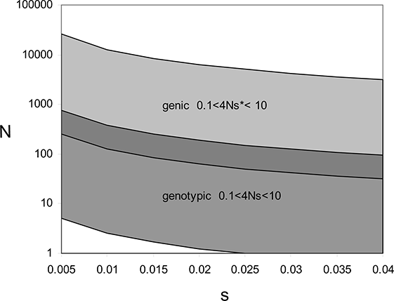
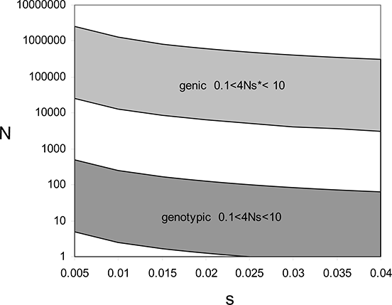
We note that the predictions of genic and genotypic models become increasingly different as p approaches 0.5. The surface that represents the critical value for the genic model (labeled A in Figure 1) approaches $p=0.5$ asymptotically but never reaches it with a finite N. Figures 2 and 3 illustrate the predictions of the genic and genotypic models in the vicinity of $p=0.5$ . In these figures we depict the regions of (N, s) space in which the critical values of 4Ns and 4Ns* are between 0.1 and 10, which, as noted above, is the conservative estimate for the regions in which the models predict that both selection and drift are likely to occur. In the regions in which the 4Ns values are larger than 10 or smaller than 0.1, the models predict the predominance of selection and drift, respectively.

Figure 2.

Here we plot the regions in which the genic and genotypic models predict that both drift and selection will occur. The two gray areas illustrate the region in which $0.1< 4Ns< 10$ for the genotypic model and $0.1< 4Ns^{*}< 10$ for the genic model, for $p=0.51$ . In the region of parameter space represented by the gray areas, the relevant model predicts that both selection and drift are likely to occur. There is a narrow band of overlap, represented by the darker gray. For each model, selection will dominate in the region above its respective band, and drift will dominate in the region below that band. Thus, for instance, in most of the region in which the genic model predicts a mix of drift and selection, the genotypic model predicts that selection will dominate.

Figure 3.

Here we plot the predictions of the genic and genotypic models as the allele frequency approaches 0.5. The two gray bands illustrate the region in which $0.1< 4Ns< 10$ for the genotypic model and $0.1< 4Ns^{*}< 10$ for the genic model for $p=0.5001$ . In the region of parameter space represented by the gray areas, the relevant model predicts that both selection and drift are likely to occur. There is no overlap of these regions. For each model, selection will dominate in the region above its respective band, and drift will dominate in the region below that band.

One might wonder if the point being made is somehow an artifact of comparing genotypic s and genic s*. It is not. We can make the same sort of comparison between two different sorts of genotypic equilibria. At the sort of equilibrium relevant to our discussion, selection actively maintains the equilibrium value. By that we mean that selection is acting at the equilibrium point. There are other sorts of genotypic equilibria. For instance, suppose that we have negative frequency-dependent selection acting on the two homozygotes AA and aa and that the heterozygote is always intermediate between the two homozygotes. (One can easily imagine plausible causal stories that would instantiate this model, e.g., predators preying on the most common phenotype.) In this situation we can assign Aa the (frequency-independent) fitness of 1. The fitness of AA is described by a line that intersects the Aa line at $p=0.5$ and has a slope of s (where p, the frequency of A, forms the horizontal axis and fitness the vertical). The fitness of aa is described by a line that intersects the Aa line at $p=0.5$ and has a slope of −s. In this model the maximal fitness difference (which occurs at $p=0$ and $p=1$ ) is s. Thus it is calibrated to compare with the genotypic model of overdominance we have been discussing, where the maximal fitness difference is also s. But in this new model the fitnesses of the three genotypes are all 1 at the equilibrium point of $p=0.5$ . Population geneticists would normally describe this as a stable equilibrium, just like the equilibrium produced by heterozygote superiority. However, the behavior of this model is not nearly as stable around the equilibrium point because there is no selection at equilibrium. To our knowledge this distinction has not been recognized by population geneticists before. We describe this difference between the two sorts of equilibrium situations by saying that the first is one that is actively maintained by selection whereas the second is not actively maintained by selection. Thus our criticism of genic selectionism can be summed up as follows: genic selectionism is committed to describing equilibria that are actively maintained by selection as equilibria in which selection is not active. But the behaviors of such equilibria differ, and there is no room for pluralism here.

Using simple population genetic models, we have pointed out how the genotypic and genic perspectives differ on the sort of equilibrium produced by heterozygote superiority. The point we are making becomes even more damning of genic selectionism when we move to models that more closely mirror reality. For instance, Nijhout (Reference Nijhout2003, Reference Nijhoutforthcoming) and Rice (Reference Rice1998, Reference Rice2004) have shown that multilocus systems, in which the phenotype is produced by realistic nonlinear developmental-genetic mechanisms, produce fitness landscapes that have long ridges instead of peaks. If one locus were allowed to drift, then because of nonlinear (= epistatic) interactions among loci, the selection regime at other loci would change. Loci that were previously highly correlated with the trait under selection (and thus themselves under selection) can become neutral, and vice versa, as the frequency of the focal locus changes. Thus the long-term predictions of the two models—one that has strong selection at the focal locus, the other that has weak or no selection at that same locus—would certainly diverge.

This dramatic divergence in predictions is not limited to cases of heterozygote superiority. Cases of heterozygote inferiority have the same result. A stable equilibrium is reached. At that equilibrium the genotypic model says that selection plus sexual reproduction maintain the equilibrium (just as in the case of heterozygote superiority; see Godfrey-Smith and Lewontin [Reference Godfrey-Smith and Lewontin1993] for a detailed discussion of the population genetics of heterozygote inferiority). In contrast, the genic selectionist is forced to say that no selection is occurring at equilibrium and thus has no resources for explaining or predicting the stability of that equilibrium point. As before, neutral theory takes over when alleles are selectively neutral and drift is the predicted outcome.

Let us briefly discuss one final case, which is less simple than the above but is of much greater generality. The case is one from quantitative genetics. Quantitative genetics deals with traits, such as height, that vary continuously, rather than discretely, and that are influenced by multiple genetic loci. The basic descriptive vocabulary of quantitative genetics includes the mean and variance of the distribution of some quantitative trait. Selection can take a number of forms, the primary ones being directional, stabilizing, and disruptive. Directional selection occurs when one extreme of the distribution is favored, for example, when taller organisms are fitter. Disruptive selection occurs when two (or more) points in the distribution are favored; for example, highest fitness is associated with organisms 2 cm tall and 7 cm tall, all other heights being selected against. Finally, stabilizing selection occurs when one point in the distribution is favored (e.g., the fittest are 5 cm tall). All three forms of selection acting on quantitative traits can result in (more or less) stable equilibria.Footnote ⁵ (The reasons for the necessity of the more or less qualification are not directly relevant to the present discussion.) We will focus on stabilizing selection, which is quite common in nature (Endler Reference Endler1986; Kingsolver et al. Reference Kingsolver2001). Imagine that we have a trait, say height, with a normal distribution in a population. This distribution has mean $\overline{X}$ and variance σ². Now let us impose artificial selection on this population by allowing only organisms within one-half of a standard deviation of the mean to reproduce. Let us assume that height in this population is influenced by a number of genetic loci and that it behaves in a way that we would expect from the experience of plant and animal breeders. After a single generation we would expect $\overline{X}$ to remain unchanged but σ² to decrease. Now we repeat (with smaller σ) and continue for a number of generations. What happens? At some point we either run out, or nearly run out, of selectable variation. Mutation should continue to introduce variation, and development is noisy, so we wouldn't really expect to get a population with zero variance in height. But we would certainly expect that maintaining this selection regime would maintain a stable equilibrium. Selection maintains the mean $\overline{X}$ and squeezes the distribution tightly around $\overline{X}$ . Thus it is responsible not only for the mean value but also for the (small) variance. It counteracts mutation and recombination among loci, which tend to increase σ².

Genic selectionists rarely, if ever, discuss cases of quantitative genetics, so it is a bit difficult to know what they would say about this case. But again their impoverished conceptual repertoire would seem to force them to say that genic selection is not occurring at this equilibrium. But if not, then drift is the expected outcome.

In this section we have shown in detail that genic and genotypic models are not empirically equivalent with respect to how they treat certain sorts of equilibrium situations. This suffices to refute any form of pluralistic genic selectionism predicated on the assumption that the two models are empirically equivalent. Given that the two models are empirically different, it follows that at most one is correct. We are confident that the genotypic model is (largely) correct and therefore that the genic model is false. This confidence is based on both empirical and theoretical reasoning. Empirically the basic model of evolutionary drift is well supported. But this is not a case of an empirically well-supported theory in which we have no idea why the theory is correct (as was true, for instance, in the time of Kepler with respect to his laws of planetary motion). The basic theory of drift derives from considerations of probabilistic sampling. The reason that there is no empirically adequate genic theory of drift is that genes are not sampled individually in diploid organisms (except in cases such as meiotic drive). In contrast, genotypes are, which is just to say that in diploid organisms the reproductive success of one gene at a locus is probabilistically tied up with that of the other gene at that locus. It would be easy to design experiments to test the different predictions of the two models with regard to the sort of equilibrium situations we have been describing. But it would not be worth the time or money since the basic theory of probabilistic sampling makes it clear that the genic theory is wrong. Supporters of genic selectionism are invited to perform the relevant experiments if they like.

2. Analysis

The first two cases, heterozygote superiority and heterozygote inferiority, are theoretically well understood. The third case from quantitative genetics is much more difficult theoretically (see Barton and Turelli Reference Barton and Turelli1989; Turelli and Barton Reference Turelli and Barton1990). Nonetheless all three cases are ones in which selection actively maintains an equilibrium. That is, were we to remove selection, the populations would drift in their state spaces. In the first two cases that state space could be described either in terms of allele frequencies or in terms of genotypic frequencies. The third case is quite different: the state space is described in terms of the mean and variance of the trait value distribution. Still in all three cases we need to invoke selection to explain stability and have a basis for predicting future stability only if we can recognize that selection is acting in each of these cases.

The genic selectionist lacks this basis. He or she, following Williams (Reference Williams1966, 59), defines the selection coefficient of an allele in a population as the weighted mean value of its fitness in its various genetic environments. According to Williams, the genetic environment of an allele includes both the other allele it is paired with at that locus and all the genes at all the other loci. In general, the definition of an allele's fitness is given as a function of its fitness in its various genetic environments weighted by the frequencies of these environments:

where ωⁱ is the fitness of the target allele in the ith genetic environment, and P _i is the relative frequency of that environment. In standard population genetic models, like our first two examples, at equilibrium different alleles at the same locus will have identical mean fitness. Although the situation is much more complex in our quantitative genetics example, it is a reasonable first approximation to say that different alleles at a locus will have identical, or nearly identical, mean fitnesses here as well.

The upshot of all this is that in the range of cases we have considered, selection is required to maintain equilibrium. However, this selection does not penetrate to the allelic level (no differential reproduction of alleles occurs). Thus the genic selectionist fails to recognize the selection that is occurring and is therefore unable to accurately predict the future evolutionary trajectory of such populations. For the genic selectionist, this is not a good thing.

We can make this point more general. If one defines fitness in terms of evolutionary consequences and one defines evolutionary consequences in terms of change (change in gene frequencies in the case of population genetics, change in mean trait value in the case of quantitative genetics), then one is doomed to make the mistake described above. To make the logic of the above even more explicit, we are assuming that a difference in fitness is a necessary condition of natural selection. Starting with Fisher (Reference Fisher1930), many have argued in favor of defining fitness in terms of evolutionary consequences (where evolutionary consequence is explicitly or implicitly defined in terms of change). Recently some have argued for a point even stronger than Fisher's; that is, not only should fitness be defined in terms of evolutionary consequences, it must be so defined (see Matthen and Ariew Reference Matthen and Ariew2002; Walsh, Lewens, and Ariew Reference Walsh, Lewens and Ariew2002). At equilibrium there is no change in the frequency of types (genotypes, genes); therefore, if one defines fitness in terms of evolutionary change (as opposed to within-generation differential reproduction), our results apply (see Brandon [Reference Brandon2006] for further discussion). The point made here is not based on some esoteric cutting-edge biological discovery, and so one might naturally wonder why it has not been recognized before. We will not try to definitively answer that question, but will briefly set out three speculative answers.

First, although the literature on this controversy is large (in addition to the papers cited above, see Sober and Wilson [Reference Sober and Wilson1998], Van der Steen and Van der Berg [Reference Van der Steen and Van den Berg1999], Lloyd [Reference Lloyd, Singh, Krimbas, Paul and Beatty2001], Gould [Reference Gould2002], and Wilson [Reference Wilson2003]), to our knowledge this paper is the first to bring drift into the discussion. So one possible answer is that philosophers (and some biologists as well) largely fail to appreciate the impact of drift on the evolutionary process.

Second, many philosophers and biologists involved in this debate seem overly concerned with the formal properties of certain models while losing sight of the fact that these models are simply tools for scientific prediction and explanation (e.g., Godfrey-Smith and Lewontin Reference Godfrey-Smith and Lewontin1993). A carpenter who becomes overly concerned with the formal properties of hammers soon becomes unemployed.

Third, it seems plausible to us that many have tacitly accepted a Newtonian view of evolution (perhaps inspired by Sober [Reference Sober1984]). In particular, many have tacitly accepted the idea that the Hardy-Weinberg Law is an analogue of Newton's principle of inertia. According to this view, the Hardy-Weinberg Law gives the zero-force condition for populations, and when in this condition, populations remain at rest. As one of us has argued elsewhere (Brandon Reference Brandon2006), this is seriously mistaken. The natural state of populations is random movement; anything other than that requires special explanation. But we cannot pursue that further here.

3. Genic Selectionist Response

If what we have presented above is correct, then genic selectionism is no longer tenable. How might the genic selectionist respond? We can think of three responses but will argue that none are satisfactory.

First, a genic selectionist might say that we have violated the rules of the game being played: that the game was one in which for any selection story being told the genic selectionist could tell an equivalent story at the genic level.Footnote ⁶ Thus far none of the stories involved drift, so we have somehow broken the rules by making drift relevant. But we haven't made drift relevant, nature has. Let us put this point differently. It would be a misunderstanding of what we have done to say that we have compared the genic selectionist account of the interaction of selection and drift with that of the genotypic selectionist. There is no genic account of drift. We have created it as a direct analogue of the genotypic account. We have done so in as sympathetic a manner as is possible (taking very conservative standards on the state space regions in which selection dominates drift etc.). But the exact quantitative details of our account can be ignored if we focus on equilibrium. There the genic selectionist is forced to say that selection is not acting, and therefore, no matter what the other parameter values, drift, and only drift, will move the population. A genic selectionist could respond to this by saying that when it comes to drift, one has to adopt genotypic selection coefficients in order to correctly predict drift/selection interactions. But that, it seems, is giving up the game.

An important positive point can be made in response to the above. In all real populations, selection and drift are intermixed. They are both part and parcel of a constitutive process of any evolutionary system, namely, the sampling process (see Brandon Reference Brandon2005, Reference Brandon2006). Thus no theory of selection can claim to be empirically adequate if it excludes drift. It is our contention that the inclusion of drift shows how the genic selectionist goes wrong in describing situations of equilibria maintained by selection.

Second, a genic selectionist might try to explain the stability of equilibria by invoking counterfactual selection. That is, although selection is not occurring at equilibrium, it would occur were the population to move away from equilibrium. From the genic perspective that is certainly true. For instance, in the case of heterozygote superiority, were the population to move from the equilibrium point at which the allelic fitnesses are identical, they would cease to be identical and selection would move the population back toward the equilibrium. However, it is hard to see how nonactual processes can maintain an equilibrium. That is, if the population does in fact remain at equilibrium (as it would be expected to if the genotypic fitness differentials are large), then the genic selectionist is forced to say that selection is not actually occurring (even though it would occur were the population to move from equilibrium). Thus there is no basis to explain the past persistence, or to predict the future persistence, of the equilibrium. To put this point more succinctly, as pointed out in Section 1, the two models predict different evolutionary trajectories. The genic selectionist cannot avoid that inconvenient fact by appealing to counterfactual selection.

Finally, there is a possible response that is not so easy to counter. This is not a response that either Dawkins or Williams would be comfortable with since they are both committed to defining allelic fitness in terms of the mean fitness of the allele across all its genetic contexts. We will give a simple example to show why Dawkins and Williams are committed to mean allelic fitness. Then we will explore a suggestion by Ken Waters that, if correct, would allow the genic selectionist to say that selection is still occurring at the sort of equilibrium situations we have been considering.

Dawkins (Reference Dawkins1976, 40ff) gives an example of choosing the best rower in crew. Our example is exactly analogous to his but has one advantage, which we will see later. It is from the less rarified world of three-legged racing. Contestants in such races come in pairs. They stand shoulder to shoulder, wrapping their interior arms around each other. Their interior legs are tied together. Hence the term “three-legged.” Suppose that we have 10 people: Alma, Bert, Clarence, Dora, Eileen, Fred, Gerhart, Hans, Inez, and Jacques. We are asked to determine the best three-legged racer of the bunch and send him or her on to the county fair. Notice that we have not been asked to determine the best three-legged racing team. That would be easy. There are 45 possible pairings of the 10 people. If that were our task, we would simply time each pair over the prescribed course and then compare their times. The fastest time would determine the best team. But we have been asked to find the best individual three-legged racer. By now you may have noticed the analogy to diploid organisms. Alleles in diploid organisms come in pairs. And if one of them does well in that organism, the other does equally well. But the genic selectionist wants to assign fitness values to individual alleles. They do so in the same way we will pick our racer for the fair.Footnote ⁷

We tie Alma and Bert together and time them over our course, then Clarence and Dora, and so on through all 45 pairs, making sure that every racer has sufficient rest between runs. The Alma-Bert time is assigned to both Alma and Bert. In the end Alma has had nine different partners, and so she has nine times. We add them and divide by nine to get her mean time. We do the same for everyone else. The person with the lowest mean time wins. This captures the ideas of both Dawkins and Williams. Although genes in a population occur in numerous genetic contexts, selection always has an arithmetic mean effect on each allele in the population. And the mean effect is its fitness (see Dawkins Reference Dawkins1976, 40ff.; Williams Reference Williams1966, 58ff.).

This makes a certain amount of sense, but, as we have seen above, it has the consequence of making the genic models predictively inaccurate in cases of stable equilibria or stabilizing selection. Waters (Reference Waters1991) argues that the genic selectionist is not stuck with defining fitness in terms of the mean effect across all genetic contexts. So in the case of heterozygote superiority we can say that there are two allelic environments, _A and _a (where _A stands for the allelic environment of having A as the allele on the homologous chromosome and _a is the environment in which a is the other allele).Footnote ⁸ A does poorly in the _A environment and well in the _a environment. Similarly for a. This, Waters suggests, is just like selection in heterogeneous environments. Imagine a sessile haploid organism that reproduces asexually by producing small buds that are distributed by the wind. The physical environment over which they are distributed is heterogeneous; it is divided into wet areas (W) and dry (D). There are two haploid genotypes, G ₁ and G ₂. G ₁ does well in W but poorly in D. G ₂ does well in D but poorly in W. What happens? Our expectation is that G ₁ and G ₂ will be maintained in the population in a stable equilibrium. And it is selection that maintains this equilibrium. Why not make the analogous case for alleles A and a in the case of heterozygote superiority?

First, Waters seems to understand the notion of environment in a particular way that makes the genic account look sensible, rather than as a real, measurable, manipulable, explanatory concept (for the outlines of that concept, see Brandon [Reference Brandon1990, Chapter 2]). Brandon has defined a homogeneous selective environment as an area within which relative fitnesses are constant. In contrast, an area is heterogeneous if across it there are $G\times E$ interactions; that is, relative fitnesses change. The wet/dry example above is indeed an example of environmental heterogeneity. We might use a simple spatial scale to measure heterogeneity or a simple temporal scale or something more complex (see Brandon Reference Brandon1990, Chapter 2). But a homogeneous environment is something that really exists in space-time. And within that region differential reproduction occurs in a (statistically) consistent way. This is what allows this notion to play the crucial theoretical role that it plays in contemporary evolutionary biology (see Brandon and Antonovics [Reference Brandon, Antonovics and Brandon1996] for discussion of three examples). And this is what allows it to be experimentally measurable (Antonovics, Ellstrand, and Brandon Reference Antonovics, Ellstrand, Brandon, Gottlieb and Jain1988). Waters' abstract construct lacks both these features.

Where is the _A environment? It cannot be the space-time worm of some particular organism, especially if that organism is heterozygote. Because then it would be the _a environment as well. It is incoherent that one and the same space-time region can be two different environments for the same selective process.Footnote ⁹ Are we looking at too high a level? Perhaps it is a part of some particular cell in an organism? But which cell? A somatic cell interacting with the external environment? A sex cell? This is clutching at straws.

But things get worse for this account. The primary problem is that differential reproduction does not occur in any of these contexts.Footnote ¹⁰ The fates of the two alleles at a locus in a diploid organism are tied together, just as Jacques and Inez in a three-legged race. Jacques may be exceedingly fast and Inez stunningly slow; but when they are tied together they get the same time. (Recall above where we argued that the genic point of view cannot give an empirically adequate account of drift because it deals with subparts of the entity being sampled. The same is true of its account of selection.) The following metaphor may be helpful. A particular selective environment is an arena for competition. We can imagine one horse consistently beating another horse on a 1-mile dry track but consistently losing to the other on a 1.5-mile wet track. Those are two different arenas for competition. Similarly one genotype of a grass may do better than another in one spot in which the soil is contaminated with lead, but 1 meter away, where the soil is uncontaminated, the fitness order of the two genotypes is reversed.Footnote ¹¹ That is how we individuate selective environments—in terms of consistency and change of relative fitness. And fitness we ultimately measure in terms of reproductive success. Thus it makes no sense to talk of a selective environment for an allele within a diploid organism (unless something like meiotic drive is going on).

And so we conclude that Waters’ suggestion is not one that is really available to the genic selectionist. The notion of selective environment it relies on is ultimately incoherent. Thus genic selectionists, and genic pluralists for that matter, are left with the coherent, but empirically inadequate, ideas of Williams and Dawkins. And thus genic selectionism and genic pluralism have been refuted.

4. Concluding Thoughts

We have focused on genic selectionism in this paper, but the argument here has a much broader scope. We have seen that any attempt to define fitness in terms of evolutionary change is doomed to the same failure as genic selectionism. Any such attempt will mistake strong selection for no selection in a range of cases. And once we decide to use the models to make genuine predictions, as opposed to treating them as objects for scholastic contemplation, this mistake will lead to empirically incorrect predictions. Thus, for instance, Fisherian fitness is not just wrong-headed, it is empirically inadequate.

Some time ago Bill Wimsatt (Reference Wimsatt1980) derided genic selectionism as mere bookkeeping. He was right. He had in mind a number of philosophical flaws in the genic selectionist approach. Not only is genic selectionism explanatory empty (Sober and Lewontin Reference Sober and Lewontin1982; Brandon Reference Brandon1990); it is entirely dissociated from real science (Lloyd Reference Lloyd2005). Here the focus has been on the more mundane. It is false.