1 Introduction
Recent technological advancements – mainly horizontal drilling and hydraulic fracturing – in the exploitation of the shale gas reservoirs have transformed the United States’ economy and energy outlook (Cueto-Felgueroso & Juanes Reference Cueto-Felgueroso and Juanes2013). With all the progress which has been made towards a better understanding of the shale (see Curtis et al. Reference Curtis, Sondergeld, Ambrose and Rai2012; Bai et al. Reference Bai, Elgmati, Zhang and Wei2013; Suleimenova et al. Reference Suleimenova, Bake, Ozkan, Valenza, Kleinberg, Burnham, Ferralis and Pomerantz2014; Cao et al. Reference Cao, Song, Wang and Xia2015; Gu et al. Reference Gu, Cole, Rother, Mildner and Brantley2015; Tahmasebi, Javadpour & Sahimi Reference Tahmasebi, Javadpour and Sahimi2015; Ma et al. Reference Ma, Zhong, Cheng, Pan, Dai, Zhang and Yang2016; Tahmasebi et al. Reference Tahmasebi, Javadpour, Sahimi and Piri2016; Zhou et al. Reference Zhou, Yan, Xue, Guo and Li2016), the production characteristics remain an enigma (Yan, Wang & Killough Reference Yan, Wang and Killough2016). Depending on the shale play, the problem has been approached by various researchers from different angles. For example Patzek, Male & Marder (Reference Patzek, Male and Marder2013) considered a no-desorption production mechanism in Barnett shale, and developed a minimal-ingredient model which could represent the large-scale gas flow characteristics through a one-dimensional (1-D) gas-diffusivity equation. Attempts also have been made to build more comprehensive multi-scale (reservoir) models which include different micro- or nano-scale phenomena in meso-scale formulations (see Akkutlu & Fathi Reference Akkutlu and Fathi2012; Yan et al. Reference Yan, Wang and Killough2016). Dissolved gas contribution to the total gas production is not included in these models, however. Reservoir material balance equations have been generalized to account for the contribution of different gas storage mechanisms such as free, adsorbed and dissolved gas in both shale gas and gas condensate reservoirs (see Lopez & Aguilera Reference Lopez and Aguilera2013; Ibarra & Aguilera Reference Ibarra and Aguilera2017). In summary, even though significant progress has been made in model development for shale reservoirs, the industry still lacks comprehensive reservoir production forecast models.
Besides the effect of fracture network pattern and connectivity on the gas flow regime, the peculiar and hard-to-predict production characteristics of shale gas reservoirs have their roots mainly in the mechanisms governing the gas storage and transport. Extremely low permeability, a considerable amount of organic matter (OM) and extremely large active surface area are the major features separating shale from conventional gas reservoirs. The past research studies on the mechanisms involved in gas transport have tremendously improved estimation of the permeability of shale gas reservoirs which has resulted in more reliable large-scale simulation studies, as did the experimental and theoretical research on the sorbed gas in estimation of original gas in place (OGIP). More details regarding each topic is presented below.
Shale gas reservoirs are extremely tight with permeability values at nano-Darcy scale. This low permeability implies pore throats of comparable size to gas molecules. As a result, new gas transport mechanisms come into play. For example, because of the nanometre pores, the no-slip assumption at the pore walls breaks down and the Knudsen diffusion contributes to the gas flow as well. Therefore, the gas permeability of shales are pressure and temperature dependent. Modelling and measurements of shale permeability has been subject to extensive research among which we can name the studies conducted by: Javadpour, Fisher & Unsworth (Reference Javadpour, Fisher and Unsworth2007), Cui, Bustin & Bustin (Reference Cui, Bustin and Bustin2009), Javadpour (Reference Javadpour2009), Civan (Reference Civan2010), Civan, Rai & Sondergeld (Reference Civan, Rai and Sondergeld2011), Darabi et al. (Reference Darabi, Ettehad, Javadpour and Sepehrnoori2012), Mehmani, Prodanović & Javadpour (Reference Mehmani, Prodanović and Javadpour2013), Singh et al. (Reference Singh, Javadpour, Ettehadtavakkol and Darabi2014), Naraghi & Javadpour (Reference Naraghi and Javadpour2015), Zhang et al. (Reference Zhang, Hu, Meegoda and Gao2015), Wu & Zhang (Reference Wu and Zhang2016).
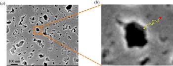
Because of the large number of small pores (figure 1) within the OM (i.e. organic pores), shales have large specific surface area (Javadpour et al. Reference Javadpour, Fisher and Unsworth2007; Ji et al. Reference Ji, Zhang, Milliken, Qu and Zhang2012; Zhang et al. Reference Zhang, Ellis, Ruppel, Milliken and Yang2012) which is covered by multiple layers or a single layer of natural gas molecules. As reservoir pressure drops the gas molecules desorb from the pore inner walls. The evolution of the adsorbed gas and its contribution to the total gas flow is usually modelled using Langmuir or Brunauer–Emmett–Teller (BET) isotherms (Yu, Sepehrnoori & Patzek Reference Yu, Sepehrnoori and Patzek2016; Wang et al. Reference Wang, Zhu, Liu and Zhang2016).
(a) A close-up scanning electron microscope image selected on OM of an Eagle Ford shale sample reveals pores of different sizes and shapes. (b) A schematic path of a diffused gas molecule from OM solid matrix towards OM pore inner wall.

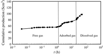
Cumulative gas production profile for sample no. 1 in Sang et al. (Reference Sang, Li, Yang, Zhu, Yao and Dong2016a ). The dotted vertical lines delineate the onset of different mechanisms contributing to the total gas flow. The fast release of free gas is followed by a slow release of adsorbed and dissolved gas.

In addition to the sorbed gas (see Ross & Bustin Reference Ross and Bustin2009; Ji et al. Reference Ji, Zhang, Milliken, Qu and Zhang2012), OM also holds a considerable amount of gas inside its solid matrix known as dissolved gas which they release at the later times of desorption process as the local pressure drops more (see Carlson & Mercer Reference Carlson and Mercer1991; Javadpour et al. Reference Javadpour, Fisher and Unsworth2007; Swami & Settari Reference Swami and Settari2012; Lopez & Aguilera Reference Lopez and Aguilera2013; Swami, Settari & Javadpour Reference Swami, Settari and Javadpour2013; Sang et al. Reference Sang, Li, Yang, Zhu, Yao and Dong2016a ; Ibarra Reference Ibarra2016; Sang et al. Reference Sang, Li, Zhu, Zhang and Dong2016b ). Etminan et al. (Reference Etminan, Javadpour, Maini and Chen2014) studied the rate of gas dissolution into OM and measured the gas diffusion coefficient. According to Yang et al. (Reference Yang, Wang, Dong, Wang, Li, Gong and Sang2016), ‘gas dissolves into the organic matter just as natural gas dissolves into heavy oil’ and gas dissolution in the OM delays the adsorption process. In other words, as soon as the gas adsorbs onto the OM pore walls it dissolves into the OM simultaneously.
OM is distributed through shale gas reservoirs and its contribution to gas storage has been proved experimentally and observed through field production data by many researchers (see Carlson & Mercer Reference Carlson and Mercer1991; Javadpour et al.
Reference Javadpour, Fisher and Unsworth2007; Swami & Settari Reference Swami and Settari2012; Lopez & Aguilera Reference Lopez and Aguilera2013; Swami et al.
Reference Swami, Settari and Javadpour2013; Etminan et al.
Reference Etminan, Javadpour, Maini and Chen2014; Ibarra Reference Ibarra2016; Ibarra & Aguilera Reference Ibarra and Aguilera2017; Sang et al.
Reference Sang, Li, Yang, Zhu, Yao and Dong2016a
,Reference Sang, Li, Zhu, Zhang and Dong
b
; Yang et al.
Reference Yang, Wang, Dong, Wang, Li, Gong and Sang2016). Studies conducted by Sang et al. (Reference Sang, Li, Yang, Zhu, Yao and Dong2016a
,Reference Sang, Li, Zhu, Zhang and Dong
b
) showed
 $6\,\%$
,
 $13\,\%$
,
 $16\,\%$
and
 $19\,\%$
relative contribution by dissolved gas to the cumulative production for different shale samples at different production pressures. Figure 2 is adopted from Sang et al. (Reference Sang, Li, Yang, Zhu, Yao and Dong2016a
) and clearly shows different gas storage mechanisms in a shale gas core sample. Etminan et al. (Reference Etminan, Javadpour, Maini and Chen2014) reported
 $22\,\%$
relative contribution by dissolved gas to the total gas production. The material balance conducted by Ibarra & Aguilera (Reference Ibarra and Aguilera2015), Ibarra (Reference Ibarra2016) for a case study of Devonian shales in the Appalachian basin showed up to
 $70\,\%$
relative contribution by dissolved gas to the total gas production. According to Ibarra & Aguilera (Reference Ibarra and Aguilera2017) dissolved gas also contributes to gas storage in shale gas condensate reservoirs but not as much as dry shale gas reservoirs. They reported
 $10.81\,\%$
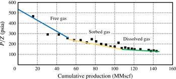
relative contribution by the dissolved gas in shale gas condensate reservoirs. Figure 3 (see Lopez & Aguilera Reference Lopez and Aguilera2013) shows the material balance plot for well no. 6654, Lincoln County, WV. Lopez & Aguilera (Reference Lopez and Aguilera2013), Ibarra & Aguilera (Reference Ibarra and Aguilera2015), Ibarra (Reference Ibarra2016) interpreted the last change in the slope in figure 3 (i.e. the green line) as indicative of a new storage mechanism (i.e. dissolved gas) in addition to the free and sorbed mechanisms which were originally pointed out by Kucuk, Alam & Streib (Reference Kucuk, Alam and Streib1978).
Material balance plot for well no. 6654, Lincoln County, WV (Lopez & Aguilera Reference Lopez and Aguilera2013). As indicated in the figure, the free gas depletes first, then the adsorbed gas and at the end the dissolved gas will be released at a much slower rate compared to free and adsorbed gas.

It is speculated that the history matching practice on shale gas reservoirs will fail if the reservoir rock is not properly characterized and the storage and transport mechanisms are not correctly identified for a given shale reservoir. Proper characterization of a given shale reservoir will help us include the essential physics governing gas transport and storage mechanisms in our reservoir models. In particular, better understanding of different gas storage mechanisms will significantly improve estimation of the relative contribution and onset of each storage mechanism to the total gas production which will eventually lead to the development of reservoir models with improved predictive capabilities.
Based on the presented experimental and theoretical works in the literature it is clear that pore level phenomena have significant control over gas molecules storage and transport. The presented literature also confirms the importance of the effects of the adsorbed and dissolved gas on the gas production rate at both core and reservoir scale. In this work we do not intend to study all the contributing mechanisms to the total gas production nor devise a comprehensive reservoir model integrating all the transport and storage mechanisms. Instead the study taps into one of the less understood - though influential – mechanisms known as: dissolved gas evolution from OM (see Lopez & Aguilera Reference Lopez and Aguilera2013; Etminan et al. Reference Etminan, Javadpour, Maini and Chen2014; Sang et al. Reference Sang, Li, Yang, Zhu, Yao and Dong2016a ,Reference Sang, Li, Zhu, Zhang and Dong b ; Ibarra Reference Ibarra2016; Ibarra & Aguilera Reference Ibarra and Aguilera2017). In this study the dissolved gas in the OM bulk and its diffusion process during pressure depletion are investigated. The dissolved gas diffuses out from the OM because of the imposed concentration gradient between organic pore surface and OM bulk due to reservoir pressure drop (see figure 1b). This process is modelled as diffusion of gas in a solid and its governing equation, which is a parabolic partial differential equation, has been solved semi-analytically over a general doubly connected domain. Without loss of generality of results, simple multi-pore models which possess a certain symmetric patterns are constructed (see § 3.3) for OM (see figure 1a) and studied systematically using the obtained analytical solution. Through those models the effects of various morphological parameters on the rate/amount of the dissolved gas produced over time are studied. It is shown that among the morphological parameters, OM specific surface area and pore size distribution have dominant effects on the gas diffusion rate of the dissolved gas. The geometry of organic pores have less influence on the rate of dissolved gas evolution compared to other morphological parameters. The length that gas molecules have to travel to be produced and the gas diffusion coefficient of the domain determine the rate of the diffusion process. For a given amount of OM in a sample with a certain porosity we can have multiple realizations with a different number of pores and pore sizes. The smaller the size of the pores, the larger the number of which have to exist within the OM for a given porosity. Specific surface area and pore size distribution are measurable and good indicators of the relative number of pores and their sizes. Because of this, the results of this study are presented in terms of these two measurable parameters rather than number of pores or pore number density. Therefore, the developed model improves our understanding of OM gas release capacity. The model can also be efficiently integrated into numerical reservoir simulators, as a source term, to include the contribution of the dissolved gas in gas production forecasts. The input model parameters include: gas diffusion coefficient, pore size and diffusion effective length. The diffusion coefficient and effective diffusion length can be obtained by following a similar approach as Etminan et al. (Reference Etminan, Javadpour, Maini and Chen2014); and the pore size distribution can be obtained from nitrogen sorption and high pressure mercury intrusion capillary pressure data as well as analysed images captured by an scanning electron microscope (SEM).
2 Model description and validation
The partial differential equation along with the boundary and initial conditions governing the gas diffusion process in OM are presented. The diffusion equation is made dimensionless and the solution procedure is explained. Thereafter, the conformal mapping functions used as part of the solution are explained in more detail. The behaviour of the solution at the pore wall (where at initial time
 $t=0$
the gas concentration is discontinuous) at the very early time is investigated. It is shown that despite the existence of spurious oscillations of the gas flow rate at the inner wall due to the well-known Gibbs phenomenon the cumulative gas flow, which is normally the measurable quantity in the laboratory, is not affected and the solution can safely be used over the entire time interval. At the end of this section the accuracy of the obtained solution is validated against numerical finite element solution of the diffusion equation over different domains.
2.1 Diffusion equation
Equation (2.1) presents the partial differential equation governing gas diffusion over the arbitrary doubly connected OM domain (
 $\unicode[STIX]{x1D6FA}_{z}$
), accompanied with inner (
 $\unicode[STIX]{x1D6FA}_{z1}$
) and outer (
 $\unicode[STIX]{x1D6FA}_{z2}$
) boundary and initial conditions where
 $C$
,
 $t$
,
 $D$
,
 $C_{0}$
and
 $\boldsymbol{n}$
are the gas concentration, time, diffusion coefficient, initial gas concentration and outward unit normal to the boundary
 $\unicode[STIX]{x2202}\unicode[STIX]{x1D6FA}_{z2}$
, respectively. The equilibrium concentration of gas at the inner pore boundary of the OM is denoted by
 $C_{eq}$
and is an input parameter to our model which comes from the desorption curves which depend on the local reservoir pressure and temperature. As the OM is surrounded by mineral grains, it is reasonable to assume no-flow boundary condition at the outer boundary of the OM. At later time of production, the rate of pressure decline and subsequently gas desorption from the surface of the OM pores is slow, hence constant gas concentration at the inner boundary is a valid assumption.
 $$\begin{eqnarray}\displaystyle \left.\begin{array}{@{}c@{}}\displaystyle \frac{\unicode[STIX]{x2202}}{\unicode[STIX]{x2202}t}C(\unicode[STIX]{x1D6FA}_{z},t)=D\unicode[STIX]{x1D6FB}^{2}C(\unicode[STIX]{x1D6FA}_{z},t),\\ \displaystyle C(\unicode[STIX]{x2202}\unicode[STIX]{x1D6FA}_{z1},t)=C_{eq},\\ \displaystyle \unicode[STIX]{x1D735}C(\unicode[STIX]{x2202}\unicode[STIX]{x1D6FA}_{z2},t)\boldsymbol{\cdot }\boldsymbol{n}=0,\\ \displaystyle C(\unicode[STIX]{x1D6FA}_{z},0)=C_{0}.\end{array}\right\} & & \displaystyle\end{eqnarray}$$
Let
 $L^{\ast }$
be the characteristic length of the physical domain
 $\unicode[STIX]{x1D6FA}_{z}$
. The Laplacian operator
 $\unicode[STIX]{x1D6FB}^{2}$
can be made dimensionless such that
 $\overline{\unicode[STIX]{x1D6FB}}^{2}={L^{\ast }}^{2}\unicode[STIX]{x1D6FB}^{2}$
. In the dimensionless Laplacian operator the derivatives are taken with respect to dimensionless spatial variables (e.g.
 $\overline{x}=x/L^{\ast },\overline{y}=y/L^{\ast },\overline{z}=z/L^{\ast }$
in a Cartesian or
 $\overline{r}=r/L^{\ast }$
in a cylindrical system of coordinates). If we replace the operator
 $\unicode[STIX]{x1D6FB}^{2}$
with its dimensionless counterpart
 $\overline{\unicode[STIX]{x1D6FB}}^{2}$
and introduce the dimensionless time and concentration as
 $\overline{t}=Dt/{L^{\ast }}^{2}$
and
 $\overline{C}=(C-C_{eq})/(C_{0}-C_{eq})$
, respectively, the dimensionless governing equation converts to (2.2).
 $$\begin{eqnarray}\displaystyle \left.\begin{array}{@{}c@{}}\displaystyle \frac{\unicode[STIX]{x2202}}{\unicode[STIX]{x2202}\overline{t}}\overline{C}(\unicode[STIX]{x1D6FA}_{z},\overline{t})=\overline{\unicode[STIX]{x1D6FB}}^{2}\overline{C}(\unicode[STIX]{x1D6FA}_{z},\overline{t}),\\ \displaystyle \overline{C}(\unicode[STIX]{x2202}\unicode[STIX]{x1D6FA}_{z1},\overline{t})=0,\\ \displaystyle \overline{\unicode[STIX]{x1D735}}\overline{C}(\unicode[STIX]{x2202}\unicode[STIX]{x1D6FA}_{z2},\overline{t})\boldsymbol{\cdot }\boldsymbol{n}=0,\\ \displaystyle \overline{C}(\unicode[STIX]{x1D6FA}_{z},0)=1.\end{array}\right\} & & \displaystyle\end{eqnarray}$$
Using the method of separation of variables the solution can be written as
 $\overline{C}(\unicode[STIX]{x1D6FA}_{z},\overline{t})=\unicode[STIX]{x1D6F9}(\unicode[STIX]{x1D6FA}_{z})T(\overline{t})$
which upon substitution into the (2.2) results in an ordinary differential equation (ODE) and an eigenvalue problem subject to the initial and boundary conditions presented in (2.2).
 $$\begin{eqnarray}\displaystyle & \displaystyle \left.\begin{array}{@{}c@{}}\displaystyle T^{\prime }(\overline{t})+\unicode[STIX]{x1D6E4}^{2}T(\overline{t})=0\\ \displaystyle \unicode[STIX]{x1D6F9}(\unicode[STIX]{x1D6FA}_{z})T(0)=1.\end{array}\right\} & \displaystyle\end{eqnarray}$$
 $$\begin{eqnarray}\displaystyle & \displaystyle \left.\begin{array}{@{}c@{}}\displaystyle \overline{\unicode[STIX]{x1D6FB}}^{2}\unicode[STIX]{x1D6F9}(\unicode[STIX]{x1D6FA}_{z})+\unicode[STIX]{x1D6E4}^{2}\unicode[STIX]{x1D6F9}(\unicode[STIX]{x1D6FA}_{z})=0\\ \displaystyle \unicode[STIX]{x1D6F9}(\unicode[STIX]{x2202}\unicode[STIX]{x1D6FA}_{z1})=0,\\ \displaystyle \overline{\unicode[STIX]{x1D735}}\unicode[STIX]{x1D6F9}(\unicode[STIX]{x2202}\unicode[STIX]{x1D6FA}_{z2})\boldsymbol{\cdot }\boldsymbol{n}=0.\end{array}\right\} & \displaystyle\end{eqnarray}$$
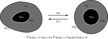
The Helmholtz equation (2.4) over doubly connected domains with a natural system of coordinates (i.e. system of coordinates which conform to the geometry of the domain) is separable, therefore it can be solved using the separation of variables method. However, for a general doubly connected region there is no system of coordinates over which the Helmholtz equation is separable. According to the doubly connected analogue of Riemann’s mapping theorem there is always a mapping function from an arbitrary doubly connected region
 $\unicode[STIX]{x1D6FA}_{z}$
in the
 $z$
-plane onto an annulus
 $\unicode[STIX]{x1D6FA}_{\unicode[STIX]{x1D709}}$
in the
 $\unicode[STIX]{x1D709}$
-plane (see figure 4). Therefore it is more convenient to transform the Helmholtz equation (2.4) on to an equivalent equation (i.e. non-constant coefficient Helmholtz equation) in the
 $\unicode[STIX]{x1D709}$
-plane, solve it there and then revert back the results onto the
 $z$
-plane if needed. Provided that we are able to find the annular domain
 $\unicode[STIX]{x1D6FA}_{\unicode[STIX]{x1D709}}$
which is conformally equivalent to the desired physical domain
 $\unicode[STIX]{x1D6FA}_{z}$
and the mapping function
 $z(\unicode[STIX]{x1D709})$
which maps
 $\unicode[STIX]{x1D6FA}_{\unicode[STIX]{x1D709}}$
onto
 $\unicode[STIX]{x1D6FA}_{z}$
, we will be able to solve the non-constant coefficient Helmholtz equation (2.6) (which is equivalent to the constant coefficient Helmholtz equation (2.4) in the
 $z$
-plane) over
 $\unicode[STIX]{x1D6FA}_{\unicode[STIX]{x1D709}}$
and then revert back the results to the
 $z$
-plane if needed (Laura & Ercoli Reference Laura and Ercoli1972).
 $$\begin{eqnarray}\displaystyle \left.\begin{array}{@{}c@{}}\displaystyle T^{\prime }(\overline{t})+\unicode[STIX]{x1D6E4}^{2}T(\overline{t})=0\\ \displaystyle \unicode[STIX]{x1D6F9}(\unicode[STIX]{x1D6FA}_{\unicode[STIX]{x1D709}})T(0)=1.\end{array}\right\} & & \displaystyle\end{eqnarray}$$
 $$\begin{eqnarray}\displaystyle \left.\begin{array}{@{}c@{}}\displaystyle \overline{\unicode[STIX]{x1D6FB}}^{2}\unicode[STIX]{x1D6F9}(\unicode[STIX]{x1D6FA}_{\unicode[STIX]{x1D709}})+\unicode[STIX]{x1D6E4}^{2}\biggl|\frac{\text{d}z}{\text{d}\unicode[STIX]{x1D709}}\biggr|^{2}\unicode[STIX]{x1D6F9}(\unicode[STIX]{x1D6FA}_{\unicode[STIX]{x1D709}})=0\\ \displaystyle \unicode[STIX]{x1D6F9}(\unicode[STIX]{x2202}\unicode[STIX]{x1D6FA}_{\unicode[STIX]{x1D709}1})=0,\\ \displaystyle \overline{\unicode[STIX]{x1D735}}\unicode[STIX]{x1D6F9}(\unicode[STIX]{x2202}\unicode[STIX]{x1D6FA}_{\unicode[STIX]{x1D709}2})\boldsymbol{\cdot }\boldsymbol{n}=0.\end{array}\right\} & & \displaystyle\end{eqnarray}$$
The black central area represents an organic pore within the OM which is illustrated in grey. The annular OM domain
 $\unicode[STIX]{x1D6FA}_{z}$
and the constant coefficient Helmholtz equation defined over it can be mapped onto the annulus
 $\unicode[STIX]{x1D6FA}_{\unicode[STIX]{x1D709}}$
and the corresponding non-constant coefficient Helmholtz equation, and vice versa.

After transformation of the Helmholtz equation from the
 $z$
-plane to the non-constant coefficient Helmholtz equation in the
 $\unicode[STIX]{x1D709}$
-plane the problem to be solved is the eigenvalue problem presented in (2.6). As the model domain
 $\unicode[STIX]{x1D6FA}_{\unicode[STIX]{x1D709}}$
is an annulus, it is reasonable and convenient to express the solution of the (2.6) in terms of double infinite series of cylindrical harmonics (2.7).
 $$\begin{eqnarray}\displaystyle \unicode[STIX]{x1D6F9}(\overline{r},\unicode[STIX]{x1D703}) & = & \displaystyle \mathop{\sum }_{n=1}^{\infty }\mathop{\sum }_{m=0}^{\infty }[Y_{m}(\unicode[STIX]{x1D6FE}_{mn}\overline{r}_{i})J_{m}(\unicode[STIX]{x1D6FE}_{mn}\overline{r})-J_{m}(\unicode[STIX]{x1D6FE}_{mn}\overline{r}_{i})Y_{m}(\unicode[STIX]{x1D6FE}_{mn}\overline{r})]\nonumber\\ \displaystyle & & \displaystyle \times \,(A_{mn}\cos m\unicode[STIX]{x1D703}+B_{mn}\sin m\unicode[STIX]{x1D703}),\end{eqnarray}$$
where the values of
 $\unicode[STIX]{x1D6FE}_{mn}$
are the roots of
 $Y_{m}(\unicode[STIX]{x1D6FE}_{mn}\overline{r}_{i})J_{m}^{\prime }(\unicode[STIX]{x1D6FE}_{mn}\overline{r}_{o})-J_{m}(\unicode[STIX]{x1D6FE}_{mn}\overline{r}_{i})Y_{m}^{\prime }(\unicode[STIX]{x1D6FE}_{mn}\overline{r}_{o})=0$
. Considering the initial and boundary conditions, it is reasonable to assume that the isoconcentrations do not deviate significantly from circles. Hence,
 $\unicode[STIX]{x1D703}$
-dependence of the solution (2.7) is so weak that we can assume that
 $m=0$
is the dominating term in the solution. Besides, given that the initial gas concentration is not a function of
 $\unicode[STIX]{x1D703}$
(i.e.
 $C_{0}$
is constant over the domain) it can be shown that (in the final solution of the diffusion equation) the coefficients
 $A_{mn}$
and
 $B_{mn}$
will be zero for any
 $m\neq 0$
. In other words, all the angular dependent terms except the first one (which corresponds to
 $m=0$
) will multiply by their corresponding zero coefficients (i.e.
 $A_{mn}=0$
and
 $B_{mn}=0$
where
 $m\neq 0$
). Therefore, we can either drop the series terms associated with
 $m\neq 0$
, from the beginning, based on the aforementioned physical reasoning, or they will be eliminated, later, after being multiplied by their associated zero coefficients
 $A_{mn}$
and
 $B_{mn}$
(where
 $m\neq 0$
). We decided to drop all the terms corresponding to
 $m\neq 0$
from the series (2.7), from the beginning, and use the obtained reduced version (2.8) in calculation of the eigenvalues of (2.6). However, if we were only interested in finding all the eigenvalues of (2.6), it would be reasonable to use the full form of (2.7) to find as many eigenvalues as possible, depending on the number of series terms used. We did these computations with the full form of (2.7) and compared the results with the numerically evaluated eigenvalues over the physical domain and a highly accurate match between the two computations was found. However, for our problem we do not need to find all the eigenvalues. We only need to find the eigenvalues which will be used/present in our final solution of the diffusion equation. Therefore, for calculation of the required eigenvalues, we used the series (2.8) which will represent the spatial part of our final solution of the diffusion equation. In § 2.4 we show that a solution based on the simplified version of (2.7) (i.e. (2.8)), still, results in accurate predictions even for highly distorted pore geometries, (see figure 6). Note if
 $C_{0}$
depended on
 $\unicode[STIX]{x1D703}$
then both the coefficients
 $A_{mn}$
and
 $B_{mn}$
(where
 $m\neq 0$
) would be non-zero. However, a non-symmetric initial condition does not represent the physics of our problem, i.e. the initial gas concentration
 $C_{0}$
is constant in the domain of interest.
Based on the presented argument, we simplify the series (2.7) and the result (i.e. the spatial part of the final solution of the diffusion equation) with a finite number of terms, becomes:
 $$\begin{eqnarray}\displaystyle \unicode[STIX]{x1D6F9}(\overline{r},\unicode[STIX]{x1D703})=\mathop{\sum }_{n=1}^{N}A_{0n}[Y_{0n}(\unicode[STIX]{x1D6FE}_{0n}\overline{r}_{i})J_{0}(\unicode[STIX]{x1D6FE}_{0n}\overline{r})-J_{0}(\unicode[STIX]{x1D6FE}_{0n}\overline{r}_{i})Y_{0}(\unicode[STIX]{x1D6FE}_{0n}\overline{r})]. & & \displaystyle\end{eqnarray}$$
If we substitute (2.8) into the non-constant coefficient Helmholtz equation (2.6) the residual (2.9) will be obtained which does not vanish since (2.8) is not the exact solution of the partial differential (2.6).
 $$\begin{eqnarray}\displaystyle \unicode[STIX]{x1D6EF}(\overline{r},\unicode[STIX]{x1D703}) & = & \displaystyle \overline{\unicode[STIX]{x1D6FB}}^{2}\unicode[STIX]{x1D6F9}(r,\unicode[STIX]{x1D703})+\unicode[STIX]{x1D6E4}^{2}\biggl|\frac{\text{d}z}{\text{d}\unicode[STIX]{x1D709}}\biggr|^{2}\unicode[STIX]{x1D6F9}(\overline{r},\unicode[STIX]{x1D703})\nonumber\\ \displaystyle & = & \displaystyle \mathop{\sum }_{n=1}^{N}A_{0n}(\unicode[STIX]{x1D6E4}^{2}\biggl|\frac{\text{d}z}{\text{d}\unicode[STIX]{x1D709}}\biggr|^{2}-\unicode[STIX]{x1D6FE}_{0n}^{2})[Y_{0n}(\unicode[STIX]{x1D6FE}_{0n}\overline{r}_{i})J_{0}(\unicode[STIX]{x1D6FE}_{0n}\overline{r})-J_{0}(\unicode[STIX]{x1D6FE}_{0n}\overline{r}_{i})Y_{0}(\unicode[STIX]{x1D6FE}_{0n}\overline{r})].\end{eqnarray}$$
To minimize the residual function (2.9) over the annulus
 $\unicode[STIX]{x1D6FA}_{\unicode[STIX]{x1D709}}$
, Galerkin’s method of weighted residuals is used which results in the following system of
 $(N+1)$
linear algebraic equations in the
 $(N+1)$
unknown constants
 $A_{0n}$
.
 $$\begin{eqnarray}\displaystyle \int _{\unicode[STIX]{x1D6FA}_{\unicode[STIX]{x1D709}}}\unicode[STIX]{x1D714}_{n}\unicode[STIX]{x1D6EF}(\overline{r},\unicode[STIX]{x1D703})\,\text{d}\unicode[STIX]{x1D6FA}_{\unicode[STIX]{x1D709}}=0,\quad n=1,2,\ldots ,N, & & \displaystyle\end{eqnarray}$$
where
 $\unicode[STIX]{x1D714}_{n}(\overline{r})=[Y_{0n}(\unicode[STIX]{x1D6FE}_{0n}\overline{r}_{i})J_{0}(\unicode[STIX]{x1D6FE}_{0n}\overline{r})-J_{0}(\unicode[STIX]{x1D6FE}_{0n}\overline{r}_{i})Y_{0}(\unicode[STIX]{x1D6FE}_{0n}\overline{r})]$
. The integrand expression in (2.10) comprises multiplication of Bessel functions of first and second kinds and their derivatives as well as the general mapping term
 $|\text{d}z/\text{d}\unicode[STIX]{x1D709}|^{2}$
, hence, the integral (2.10) is approximated numerically. The system of (2.10) has a non-trivial solution only if the determinant of the coefficients is zero. The determinantal equation is used to obtain the values of
 $\unicode[STIX]{x1D6E4}_{n}^{2}$
. After finding the
 $\unicode[STIX]{x1D6F9}(\unicode[STIX]{x1D6FA}_{\unicode[STIX]{x1D709}})$
functions and the values of
 $\unicode[STIX]{x1D6E4}^{2}$
which satisfy (2.6) the time ODE can be solved which leads to the final solution (2.11)
 $$\begin{eqnarray}\displaystyle \overline{C}(\overline{r},\overline{t})=\mathop{\sum }_{n=1}^{\infty }A_{0n}\unicode[STIX]{x1D714}_{n}(\overline{r})\text{e}^{-\unicode[STIX]{x1D6E4}_{n}^{2}\overline{t}}. & & \displaystyle\end{eqnarray}$$
The coefficients
 $A_{0n}$
are obtained from the initial condition:
 $$\begin{eqnarray}\displaystyle A_{0n}=\frac{2}{[\overline{r}_{0}^{2}\,f_{1}^{2}-\overline{r}_{i}^{2}f_{2}^{2}]}\int _{\overline{r}_{i}}^{\overline{r}_{o}}\unicode[STIX]{x1D714}_{n}(\overline{r})\overline{r}\,\text{d}\overline{r}, & & \displaystyle\end{eqnarray}$$
where
 $$\begin{eqnarray}\displaystyle & \displaystyle f_{1}=Y_{0}(\unicode[STIX]{x1D6FE}_{0n}\overline{r}_{i})J_{0}(\unicode[STIX]{x1D6FE}_{0n}\overline{r}_{o})-J_{0}(\unicode[STIX]{x1D6FE}_{0n}\overline{r}_{i})Y_{0}(\unicode[STIX]{x1D6FE}_{0n}\overline{r}_{o}), & \displaystyle\end{eqnarray}$$
 $$\begin{eqnarray}\displaystyle & \displaystyle f_{2}=Y_{0}(\unicode[STIX]{x1D6FE}_{0n}\overline{r}_{i})J_{0}^{\prime }(\unicode[STIX]{x1D6FE}_{0n}\overline{r}_{i})-J_{0}(\unicode[STIX]{x1D6FE}_{0n}\overline{r}_{i})Y_{0}^{\prime }(\unicode[STIX]{x1D6FE}_{0n}\overline{r}_{i}). & \displaystyle\end{eqnarray}$$
In this study we are interested in the rate and cumulative production of the dissolved gas rather than the concentration profile of the dissolved gas. Hence the obtained solution is converted back to the dimensional form from which the flux (
 $J_{g}$
), flow rate (
 $q_{g}$
) and cumulative production (
 $Q_{g}$
) of the dissolved gas diffusing out from the OM pore inner walls will be obtained. Note that the internal and external boundaries of
 $\unicode[STIX]{x1D6FA}_{\unicode[STIX]{x1D709}}$
correspond to the internal and external boundaries of the physical domain
 $\unicode[STIX]{x1D6FA}_{z}$
, hence, the calculated cumulative dissolved gas production from the OM pore surface can be directly used for the physical domain.
 $$\begin{eqnarray}\displaystyle & \displaystyle J_{g}(r,\overline{t})=D\frac{\unicode[STIX]{x2202}C}{\unicode[STIX]{x2202}r}=D\frac{C_{0}-C_{eq}}{L^{\ast }}\mathop{\sum }_{n=1}^{\infty }\unicode[STIX]{x1D6FE}_{0n}A_{0n}\unicode[STIX]{x1D714}^{\prime }(\overline{r})\text{e}^{-\unicode[STIX]{x1D6E4}_{n}^{2}\overline{t}} & \displaystyle\end{eqnarray}$$
 $$\begin{eqnarray}\displaystyle & \displaystyle q_{g}(r,\overline{t})=\int _{0}^{2\unicode[STIX]{x03C0}}J_{g}(r,\unicode[STIX]{x1D703})r\,\text{d}\unicode[STIX]{x1D703}=2\unicode[STIX]{x03C0}rD\frac{C_{0}-C_{eq}}{L^{\ast }}\mathop{\sum }_{n=1}^{\infty }\unicode[STIX]{x1D6FE}_{0n}A_{0n}\unicode[STIX]{x1D714}^{\prime }(\overline{r})\text{e}^{-\unicode[STIX]{x1D6E4}_{n}^{2}\overline{t}} & \displaystyle\end{eqnarray}$$
 $$\begin{eqnarray}\displaystyle & \displaystyle Q_{g}(r,\overline{t}_{s},\overline{t}_{e})=\int _{t_{s}}^{t_{e}}q_{g}(r,t)\,\text{d}t=2\unicode[STIX]{x03C0}rL^{\ast }(C_{0}-C_{eq})\mathop{\sum }_{n=1}^{\infty }\frac{\unicode[STIX]{x1D6FE}_{0n}}{\unicode[STIX]{x1D6E4}_{n}^{2}}A_{0n}\unicode[STIX]{x1D714}^{\prime }(\overline{r})(\text{e}^{-\unicode[STIX]{x1D6E4}_{n}^{2}\overline{t}_{s}}-\text{e}^{-\unicode[STIX]{x1D6E4}_{n}^{2}\overline{t}_{e}}),\hspace{24.0pt} & \displaystyle\end{eqnarray}$$
where
 $\unicode[STIX]{x1D714}^{\prime }(\overline{r})=Y_{0}(\unicode[STIX]{x1D6FE}_{0n}\overline{r}_{i})J_{0}^{\prime }(\unicode[STIX]{x1D6FE}_{0n}\overline{r})-J_{0}(\unicode[STIX]{x1D6FE}_{0n}\overline{r}_{i})Y_{0}^{\prime }(\unicode[STIX]{x1D6FE}_{0n}\overline{r})$
.
The advantage of using the conformal mapping technique over the alternative numerical solution is that it allows us to have an analytical solution (i.e. (2.16)) at the end which can be integrated with numerical reservoir simulators as a source term. The overall/average properties of OM morphology and pore structure from a shale gas reservoir can be obtained from SEM images and be used as input to the proposed analytical model. Numerical solution of the diffusion equation integrated with reservoir simulators is extremely computationally expensive and impractical for field-scale simulation. Having an analytical solution which runs in a fraction of second and honours the average pore morphology and structure observed through SEM images will significantly improve our reservoir production forecast while keeping the computational cost low.
2.2 Mapping function
It is well known (Henrici Reference Henrici1993, p. 445) that for any non-degenerate doubly connected region
 $\unicode[STIX]{x1D6FA}_{z}$
there exists a one-to-one analytic mapping function that maps
 $\unicode[STIX]{x1D6FA}_{z}$
onto an annulus
 $\unicode[STIX]{x1D6FA}_{\unicode[STIX]{x1D709}}$
. Since the doubly connected domain
 $\unicode[STIX]{x1D6FA}_{z}$
is usually given, it is more intuitive to find the mapping function from the given domain to its corresponding annulus. However, depending on the application, it might be more convenient and useful to find the conformally equivalent annular domain to the given domain and then the mapping function from that annulus to its corresponding physical domain in the
 $z$
-plane. In this study, since we would like to calculate the mapping term
 $|\text{d}z/\text{d}\unicode[STIX]{x1D709}|^{2}$
, the latter approach is used to obtain an explicit/implicit mapping function from
 $\unicode[STIX]{x1D6FA}_{\unicode[STIX]{x1D709}}$
to
 $\unicode[STIX]{x1D6FA}_{z}$
. There are various computational methods to determine such mapping functions. For more information the reader is encouraged to view Laura (Reference Laura1965), Henrici (Reference Henrici1979), Fornberg (Reference Fornberg1984), DeLillo & Pfaltzgraff (Reference Delillo and Pfaltzgraff1998) and the references therein. In this study the DeLillo & Pfaltzgraff (Reference Delillo and Pfaltzgraff1998) procedure accompanied by consideration of the symmetry features of the domain from the work of Laura (Reference Laura1965) are used to find the conformal annulus for a given doubly connected domain as well as its mapping function in the form of a Laurent series. The presented procedure in DeLillo & Pfaltzgraff (Reference Delillo and Pfaltzgraff1998) demonstrates how to handle regions with smooth spline fitted boundaries, which is useful when algebraic equations for boundaries are not available and the information regarding the boundaries are raw coordinate data extracted from image processing.
A few simple geometries for pores in OM will suffice to better understand the effect of OM morphology on the cumulative production of the diffused gas over time. Nevertheless, more complicated domains can be handled by following the same procedure. Simple pore geometries including circle, ellipse, slit-like ellipse, square, rectangle and elongated rectangle are modelled using the superellipse (2.18).
 $$\begin{eqnarray}\displaystyle \left(\frac{x-a}{r_{a}}\right)^{2n}+\left(\frac{y-b}{r_{b}}\right)^{2n}=1, & & \displaystyle\end{eqnarray}$$
where
 $r_{a}$
,
 $r_{b}$
are superellipse semi-axes and
 $a$
and
 $b$
are the superellipse centre coordinates. The transition from elliptical shape to rectangle with sharp corners is controlled through parameter
 $n$
. The larger the value of
 $n$
the sharper the corners become.
Since the mapping function defined over the annulus
 $\unicode[STIX]{x1D6FA}_{\unicode[STIX]{x1D709}}$
is analytic, it can be represented by its Laurent series (2.19). The task is to determine suitable coefficients
 $a_{\unicode[STIX]{x1D708}}$
. Although using an explicit mapping function in the form of a power series is more convenient, its efficient usage is limited to domains with near circular shapes, such as ellipse and regular polygons, because otherwise a large number of series terms has to be used to build a sufficiently accurate mapping function (Schinzinger & Laura Reference Schinzinger and Laura1991, p. 99).
 $$\begin{eqnarray}\displaystyle z(\unicode[STIX]{x1D709})=\mathop{\sum }_{\unicode[STIX]{x1D708}=-\infty }^{+\infty }a_{\unicode[STIX]{x1D708}}\unicode[STIX]{x1D709}^{\unicode[STIX]{x1D708}},\quad \unicode[STIX]{x1D709}\in \unicode[STIX]{x1D6FA}_{\unicode[STIX]{x1D709}}. & & \displaystyle\end{eqnarray}$$
It can be proved (Laura Reference Laura1965; Laura & Ercoli Reference Laura and Ercoli1972) that the mapping function (2.19) for domains with
 $s$
axes of symmetry reduces to:
 $$\begin{eqnarray}\displaystyle z(\unicode[STIX]{x1D709})=\mathop{\sum }_{\unicode[STIX]{x1D708}=-\infty }^{+\infty }a_{1-s\unicode[STIX]{x1D708}}\unicode[STIX]{x1D709}^{1-s\unicode[STIX]{x1D708}},\quad \unicode[STIX]{x1D709}\in \unicode[STIX]{x1D6FA}_{\unicode[STIX]{x1D709}}. & & \displaystyle\end{eqnarray}$$
Equation (2.20) can be tailored even further for more specific domains. For example the mapping function (2.21) maps an annulus of outer radius 1 and inner radius
 $r_{i}=R/(a_{p}A_{s})$
in the
 $\unicode[STIX]{x1D709}$
-plane onto a regular polygon with
 $s$
axes of symmetry and apothem
 $a_{p}$
with a concentric circular hole of radius
 $R$
(Laura & Susemihl Reference Laura and Susemihl1973).
 $$\begin{eqnarray}\displaystyle \left.\begin{array}{@{}c@{}}\displaystyle z(\unicode[STIX]{x1D709})=a_{p}A_{s}\left(\unicode[STIX]{x1D709}+\mathop{\sum }_{n=1}^{\infty }a_{n}\unicode[STIX]{x1D709}^{ns+1}\right),\\ \displaystyle A_{s}=\frac{1}{1+\displaystyle \mathop{\sum }_{n=1}^{\infty }a_{n}},\\ \displaystyle a_{n}=\frac{2(2+s)(2+2s)\ldots (2+(n-1)s)}{s^{n}n!(1+ns)}(-1)^{n}.\end{array}\right\} & & \displaystyle\end{eqnarray}$$
Although the process of finding the mapping function (i.e. the coefficient in the Laurent series) is reasonably fast (
 ${<}$
10 s), leveraging the symmetry feature of the given domain lets us save only the relevant absolutely non-zero coefficients for later use in calculation of the mapping term
 $|\text{d}z/\text{d}\unicode[STIX]{x1D709}|^{2}$
in the residual (2.9) which speeds up numerical integration of (2.10).
2.3 Validation: circular pore
The developed solution is validated against the numerical solution of the diffusion equation over domains with different pore geometries. The obtained results are used in the subsequent sections to study the effect of pore geometry on the evolution of the dissolved gas over production time.
Let a circular domain of area
 $4~\unicode[STIX]{x03BC}\text{m}^{2}$
with a circular pore of area
 $1~\unicode[STIX]{x03BC}\text{m}^{2}$
be the annular OM domain
 $\unicode[STIX]{x1D6FA}_{z}$
of area
 $3~\unicode[STIX]{x03BC}\text{m}^{2}$
(see figure 5
a) and gas diffusion coefficient
 $D=10^{-20}~\text{m}^{2}~\text{s}^{-1}$
(see Etminan et al.
Reference Etminan, Javadpour, Maini and Chen2014). In such a case, since the physical domain is an annulus the mapping function becomes an identity map
 $z(\unicode[STIX]{x1D709})=\unicode[STIX]{x1D709}$
and the mapping term in the residual (2.9) becomes
 $|\text{d}z/\text{d}\unicode[STIX]{x1D709}|^{2}=1$
which leads us to the conclusion that
 $\unicode[STIX]{x1D6E4}_{0n}^{2}=\unicode[STIX]{x1D6FE}_{0n}^{2},n=1,2,\ldots ,N$
.
The gas concentration at the inner boundary is considered to be
 $1~\text{mol}~\unicode[STIX]{x03BC}\text{m}^{-2}$
and the initial gas concentration of the OM is
 $10~\text{mol}~\unicode[STIX]{x03BC}\text{m}^{-2}$
, hence, the initial (i.e.
 $t=0$
) gas concentration profile at the pore surface is discontinuous (see figure 5
b). Due to this discontinuity the slope
 $\unicode[STIX]{x2202}C/\unicode[STIX]{x2202}r$
at
 $r=r_{i}$
(i.e. pore surface) is infinite and subsequently the gas flow rate (2.16) at the pore surface at
 $t=0$
is expected to tend to infinity at the very early times. If we plot several profiles of gas flow rate at the pore surface versus time (figure 5
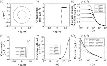
c), each corresponding to a solution comprising a different number of Fourier terms, it can be shown that the profiles corresponding to the solutions with higher number of Fourier terms predict higher gas flow rate at early times. This was expected as the solutions with higher number of Fourier terms are more accurate in prediction of the gas concentration profile (figure 5
d) and subsequently the aforementioned infinite slope
 $\unicode[STIX]{x2202}C/\unicode[STIX]{x2202}r$
and gas flow rate
 $2\unicode[STIX]{x03C0}rD\unicode[STIX]{x2202}C/\unicode[STIX]{x2202}r$
at the pore surface at early times. This discontinuity also causes the well-known Gibbs phenomenon which manifests itself at very early times as spurious oscillations in concentration profile (especially at the point of discontinuity) which do not diminish by increasing the number of Fourier terms.
(a) A schematic OM with a circular pore; (b) initial gas concentration along the
 $x$
-axis; (c) prediction of infinite flow rate at time zero at the pore surface; (d) sensitivity of the gas concentration profile to the number of Fourier terms after sufficiently large time (at
 $10^{5}~(\text{s})$
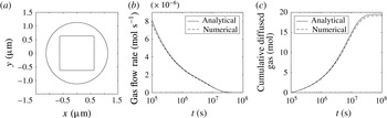
); (e) the infinite flow rate at time zero and the Gibbs phenomenon at very early times do not affect the cumulative flow of gas; (f) as the number of elements increases the numerical solution approaches the exact analytical solution.

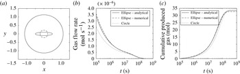
(a) OM with elongated elliptical pore; (b) there is a good match between the numerical and analytical prediction when the pore is a slit shape ellipse and the circular pore with the same area presents a different flow rate profile; (c) however, the cumulative gas flow profiles for both the circular and slit shape pore are close.

According to figure 5(c), at the very early times, the gas flow rate is a function of the number of Fourier terms used in the solution, and all the solutions collapse to one solution almost at
 $t=10^{5}$
s (
 ${\approx}$
1 day), which can still be considered as very early time as the complete gas depletion of OM (in this case) takes
 $10^{8}$
s (
 ${>}$
3 years). Nevertheless, figure 5(e) demonstrates that although the gas flow rate at very early times is a function of the number of Fourier terms, this dependency does not exist in the cumulative diffused gas (which is a more important parameter than flow rate as it is directly measurable) and all the solutions with
 $10$
or more Fourier terms have collapsed onto one solution profile along the entire time interval
 $1~\text{s}<t<10^{8}~\text{s}$
. Specifically, it is shown that the prediction of cumulative flow by 10 Fourier terms is almost identical to the prediction using 100 terms. In addition, figure 5(e) shows that the mass is conserved as the final plateau of the cumulative gas flow is equal to the total amount of the gas which could diffuse out before reaching the equilibrium condition:
 $3~\unicode[STIX]{x03BC}\text{m}^{2}\times (10-1)\text{mol}~\unicode[STIX]{x03BC}\text{m}^{-2}=27~\text{mol}$
. In conclusion, the solution can safely be used along the entire time interval.
The exact analytical solution is compared with the finite element solution and it is shown (in figure 5 f) that as the number of finite elements increases the numerical solution approaches to the analytical solution.
It is interesting to mention that it takes
 $10^{5}~\text{s}$
(
 ${\approx}$
1 day),
 $10^{7}~\text{s}$
(
 ${\approx}$
100 days) and
 $10^{8}~\text{s}$
(
 ${\approx}$
3 years) to produce 3 %, 50 % and 100 % of the total producible dissolved gas in the OM under study.
2.4 Validation: non-circular pores
In § 2.3, it was shown that the proposed general approximate semi-analytical solution degenerates to an exact semi-analytical solution when the physical domain is an annulus. The properties of the solution were studied and the solution’s validity was confirmed against the numerical solution. In this section, physical domains with non-circular pore geometries are considered and the accuracy of the solution over each domain is investigated.
A circular OM domain of area
 $4~\unicode[STIX]{x03BC}\text{m}^{2}$
with a slit-like elliptical pore whose semi-axes are
 $r_{a}=0.5~\unicode[STIX]{x03BC}\text{m}$
and
 $r_{b}=0.1~\unicode[STIX]{x03BC}\text{m}$
is considered (figure 6
a). The molar gas diffusion and cumulative diffusive gas flow versus time using the analytical and numerical solutions are shown in figure 6(b,c), respectively. It is shown that, although the pore geometry is considerably deviated from a circle, still there is a very good match between the analytical and numerical predictions. On the same OM domain a circular pore with the same area as the slit-like superellipse is considered. The circular pore has the same cross-sectional area as the elliptical pore, but it provides less circumferential area for the gas to diffuse out. Hence, as is shown in figure 6(b) the circular pore produces gas at a lower flow rate. Although the molar gas flow rate profiles for circular and elliptical pores are quite distinguishable, their cumulative flows (which is normally the measurable quantity in the laboratory) are approximately similar. The importance of pore geometry is discussed in more detail in the next section.
Superellipse parameters for different pore geometries. OM porosity is
 $25$
% except the listed one.


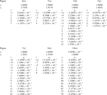
For better assessment of the accuracy and range of applicability of the proposed analytical solution five more cases with larger pore sizes compared to the previous ones are considered. All the pores are modelled using the superellipse equation and the superellipse parameters used for each case are listed in table 1. Based on the inner and outer boundary equation the mapping function for each case is obtained and listed in table 2. Each column of the table is labelled with the figure number of the corresponding domain and it has two sub-columns which shows the corresponding mapping functions’ Laurent series exponents and coefficients respectively. The area of all circular OM domains is
 $4~\unicode[STIX]{x03BC}\text{m}^{2}$
and the pore area of the first four cases is
 $1~\unicode[STIX]{x03BC}\text{m}^{2}$
and the pore area of the fifth case is
 $1.6~\unicode[STIX]{x03BC}\text{m}^{2}$
. In other words, the OM porosity for the first four cases is
 $25\,\%$
and for the fifth case is
 $40\,\%$
. Note that the first four cases have both the same volume-based total organic carbon (
 $\text{TOC}_{v}$
) and the same weight-based total organic carbon (
 $\text{TOC}_{w}$
). The
 $\text{TOC}_{v}$
of the fifth case is equal to the
 $\text{TOC}_{v}$
of the first four cases but its
 $\text{TOC}_{w}$
is less than that of the first four cases. The gas diffusion coefficient in all the cases is
 $10^{-20}~\text{m}^{2}~\text{s}^{-1}$
.
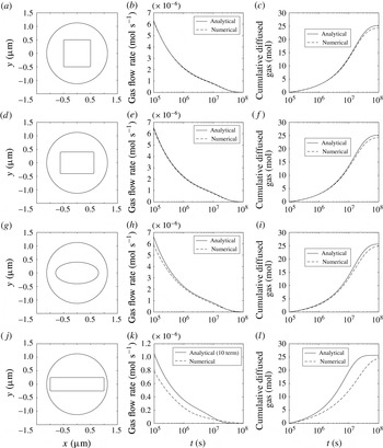
The first column illustrates different pore shapes in a circular OM domain, while the second and third columns are the corresponding temporal gas flow rate and cumulative diffused gas, respectively.

Even for a very large square pore there is a good match between the analytical and numerical solutions.

Reviewing figure 7 from top to bottom we can see a pattern that the further a pore geometry is elongated in one direction the greater the discrepancy between the analytical and the numerical solutions in both the molar gas flow and the cumulative gas flow observed. For example, in the first two cases (figure 7 a,d) the numerical and analytical solutions match very well as depicted in figure 7(b,c,e,f). However, in the third case (figure 7 g) since the pore geometry is slightly more deviated from a circular pore compared to the first two cases, a small discrepancy between the numerical and the analytical molar and cumulative gas flow rates has occurred (figure 7 h,i). In figure 7(j) since the pore geometry is considerably deviated from circle the dominant flow regime is not radial anymore and it is rather linear and perpendicular to the long edge of the rectangle. Hence, as shown in figure 7(k,l), the analytical solution for the case with highly elongated rectangular pore does not produce as accurate analytical solutions as it did in the previous cases. In the fifth case (figure 8) a very large square pore is considered and it is shown that the analytical solution for both molar gas flow and cumulative gas flow match their numerical counterparts very well. In conclusion, the proposed analytical solution has shown a very good match with the numerical solution over a wide range of cases with different pore geometries except when the pore was a relatively large and elongated rectangle which made the isoconcentrations significantly deviated from circular geometry.
3 Dissolved gas evolution analysis
In this section the effect of pore geometry, porosity, pore size distribution and specific surface area of the pores in OM on the rate of production of the dissolved gas are studied.
3.1 Effect of pore geometry
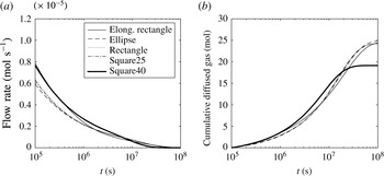
The gas molar flow rate profiles and cumulative gas flow profiles for previously studied OM domains (figure 7
a,d,g,j and 8
a) are assembled in figure 9(a,b), respectively. The OM with an elongated rectangular pore (figure 7
j) and the OM with a large square pore (figure 7
a) – because of their larger pore circumferential area compared to other cases have shown higher molar gas flow rates and cumulative gas flows at the early times (
 ${\approx}$
10 days). Since the
 $\text{TOC}_{w}$
for the OM with
 $40\,\%$
porosity is less than other OM domains (
 $25\,\%$
porosity) it has less gas content and it reaches to a lower ultimate cumulative gas (figure 9
b). Although all five cases have the same
 $\text{TOC}_{v}$
, the OM with
 $40\,\%$
porosity depletes (i.e. reaches to plateau) earlier than the OM with porosity of
 $25\,\%$
. In conclusion, although pore geometry has shown some effects on the rate of production of the dissolved gas, we can see in figure 9(b) that all the cumulative gas flow profiles are twisting around each other and following one trajectory. The OM with
 $40\,\%$
porosity would have reached the same plateau if its
 $\text{TOC}_{w}$
was equal to other cases.
(a) OM with
 $40\,\%$
porosity (represented as Square40) has the same
 $\text{TOC}_{v}$
as other cases, but because of higher porosity it produces its gas content faster; (b) OM with the same
 $\text{TOC}_{w}$
and
 $\text{TOC}_{v}$
but different pore geometries have shown very close cumulative gas production profiles; Square40 reaches plateau at a lower value because of its lower
 $\text{TOC}_{w}$
, i.e. gas content compared to others.

3.2 Effect of diffusion coefficient and OM length scale
Depending on the gas diffusion coefficient and OM length scale (while the boundary conditions are kept unaltered) the dissolved gas could be produced over the early stages of production or it may take several years. Clearly the greater the diffusion coefficient, the earlier onset of the diffusion process and faster contribution of dissolved gas to the total gas production could occur. As a rule of thumb, the time scale
 $\unicode[STIX]{x1D70F}={L^{\ast }}^{2}/D$
represents the time required for a gas molecule to travel the distance
 $L^{\ast }$
through a medium where the gas diffusion coefficient is
 $D$
. If the gas diffusion coefficient is
 $10^{-20}~\text{m}^{2}~\text{s}^{-1}$
and the length scale of the OM is
 $1~\unicode[STIX]{x03BC}\text{m}$
, it takes on average more than three years for a gas molecule to travel the distance
 $L^{\ast }$
and reach to the OM pore surface to be produced. Therefore, more pores within a OM patch creates shorter distance for a gas molecule to travel before being produced. This is discussed in more detail in the next section.
3.3 Effect of pore size distribution and specific surface area
For a given shale sample with known
 $\text{TOC}_{w}$
,
 $\text{TOC}_{v}$
and OM porosity, the temporal cumulative gas flow profile can be considerably different depending on the specific surface area and pore size distribution of the pores.
In an experiment involving convective–diffusive mass transport process, Sparrow & Ortiz (Reference Sparrow and Ortiz1982) showed that an equilateral pattern of pores within a substrate results in no-flow hexagonal boundary around each pore. This property is leveraged in this study to construct and study multi-pore OM using the analytical model developed for single pore OM. The naturally occurring no-flow boundaries divide the domain into isolated single pore hexagonal OM modules. Therefore, the developed analytical solution can be applied to one module and multiply the result by the number of modules in the OM patch in order to calculate the overall response of the domain.
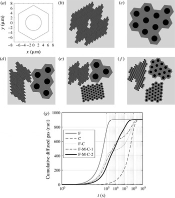
(a) A hexagonal OM of total area
 $133~\unicode[STIX]{x03BC}\text{m}^{2}$
and pore area
 $33~\unicode[STIX]{x03BC}\text{m}^{2}$
(the amount of OM is
 $100~\unicode[STIX]{x03BC}\text{m}^{2}$
); (b) 10 000 OM modules (fine: F) each containing
 $0.01~\unicode[STIX]{x03BC}\text{m}^{2}$
OM; (c)
 $10$
OM modules (coarse: C) each containing
 $10~\unicode[STIX]{x03BC}\text{m}^{2}$
OM; (d) half and half combination of modules each containing
 $0.01$
and
 $10~\unicode[STIX]{x03BC}\text{m}^{2}$
OM (C-F); (e) an equal ratio combination of modules each containing either
 $0.01$
(F),
 $0.1$
(middle: M) or
 $10~\unicode[STIX]{x03BC}\text{m}^{2}$
(C) OM (F-M-C-1); (f) an equal ratio combination of modules each containing either
 $0.02$
,
 $0.2$
or
 $2~\unicode[STIX]{x03BC}\text{m}^{2}$
OM (F-M-C-2); (g) the larger the specific surface area the earlier the dissolved gas content will be produced. For a bimodal pore size distribution with contrast between the pore sizes a two-stage production behaviour might be observed where at the first stage the gas molecules which are tens of nanometres away from the pore surfaces will be produced and then the gas molecules which are thousands of nanometres away will be produced. Multi-stage production hampers in cases where pore size distribution is wide but contrasts are low, e.g. case F-M-C-2.

Assume the total surface of bulk OM in a given rock sample is
 $100~\unicode[STIX]{x03BC}\text{m}^{2}$
and its porosity is
 $25\,\%$
. This amount of OM can exist as one hexagonal module of area
 $133~\unicode[STIX]{x03BC}\text{m}^{2}$
with a circular pore of area
 $33~\unicode[STIX]{x03BC}\text{m}^{2}$
as illustrated in figure 10(a). Consider five different rock samples each containing
 $100~\unicode[STIX]{x03BC}\text{m}^{2}$
of OM
 $25\,\%$
porosity. All five samples have the same
 $\text{TOC}_{w}$
and also the same
 $\text{TOC}_{v}$
but different morphologies. Case 1: all OM patches are made up of fine (F) modules of area
 $0.01~\unicode[STIX]{x03BC}\text{m}^{2}$
(figure 10
b). Case 2: all OM patches are composed of coarse (C) modules of area
 $10~\unicode[STIX]{x03BC}\text{m}^{2}$
(figure 10
c). Case 3: half of the total OM is composed of fine modules of area
 $0.01~\unicode[STIX]{x03BC}\text{m}^{2}$
and the other half is composed of coarse modules of area
 $10~\unicode[STIX]{x03BC}\text{m}^{2}$
(F-C in figure 10
d). Case 4: one third of the total OM is made up of fine modules of area
 $0.01~\unicode[STIX]{x03BC}\text{m}^{2}$
, one third composed of middle (M) size module of area
 $0.1~\unicode[STIX]{x03BC}\text{m}^{2}$
and one third is composed of coarse modules of area
 $10~\unicode[STIX]{x03BC}\text{m}^{2}$
(F-M-C-1 in figure 10
e). Case 5: one third of the total OM is made up of fine modules of area
 $0.02~\unicode[STIX]{x03BC}\text{m}^{2}$
, one third composed of middle size module of area
 $0.2~\unicode[STIX]{x03BC}\text{m}^{2}$
and one third is composed of coarse modules of area
 $2~\unicode[STIX]{x03BC}\text{m}^{2}$
(F-M-C-2 in figure 10
f). Since the OM content of all the samples is equal, their cumulative gas flow profiles all level off at the same value (
 $900~\text{mol}$
) as depicted in figure 10(g). Although the porosity of OM in all the samples is
 $25\,\%$
, because of different OM pore specific surface areas, sample 10(b) produces its dissolved gas in approximately
 $4$
days (
 $3.3\times 10^{5}$
s) whereas it takes approximately
 $10$
years (
 $3.3\times 10^{8}$
s) for sample 10(c) to produce all of its dissolved gas. It is worth mentioning that the specific surface area of pores in sample 10(b) is
 $1000^{0.5}$
(
 ${\approx}$
32) times larger than the pore specific surface area of sample 10(c). The OM in sample 10(d) is a combination of samples 10(b,c) and because of bimodal heterogeneity in pore specific surface area of the OM its cumulative gas profile showed a two-stage production mechanism where at the first stage both OM patches produce gas and in the second stage the OM with smaller pore specific surface area contribute to production. As we go towards a narrower and more homogeneous pore size distribution the cumulative dissolved gas flow profile shows more monotonic behaviour, e.g. samples 10(e,f) and their corresponding cumulative gas flow profiles. For a real OM patch, heterogeneity in the size of organic pores results in a complex morphology which hosts diffusion processes at different length scales. In this study diffusion processes are split and isolated depending on their length scale. This practice does not influence the gas molar conservation, however, it renders a two-stage production (F-C) more pronounced as it assumes the diffusion process occurring at the smaller scale (F) stops contributing to the flow after a while. Nevertheless, isolating diffusion processes based on their length scale is always guaranteed to yield an overall delay in production of the total dissolved gas, (i.e. our production forecast for the dissolved gas will be inherently conservative) while the final produced mole of gas is conserved. In summary, based on the results of the conducted simulations the effect of pore geometry compared to other factors has the least influence on the rate of production of the dissolved gas. However, the organic matter pore size distribution and specific surface area can significantly influence the rate of production of the dissolved gas by orders of magnitude. Therefore, reservoir production forecast based on the mere knowledge of TOC and OM porosity results in inaccurate predictions. For example the bimodal pore size distribution of OM might cause a level off in the middle of the cumulative production curve which can erroneously be perceived as a complete depletion signature. At reservoir scale as the pressure drop reaches new areas of the reservoir, new OM sources will be activated which add flow to the previously producing OM and this might introduce a surge (similar to curves F-C and F-M-C-1) in the total production rate which might cause a similar multistage production mechanism as well.
4 Concluding remarks
Sharp production decline in the early life of a gas-producing well in a shale gas reservoir followed by extended production at a low rate suggests different gas production processes at different time periods. These processes include gas production from pressurized pores at early stages followed by gas desorption and then gas diffusion processes (Javadpour et al. Reference Javadpour, Fisher and Unsworth2007). Detailed and meticulous experiments by Etminan et al. (Reference Etminan, Javadpour, Maini and Chen2014) showed these processes in the laboratory and quantified the contribution of each process on gas production. Etminan et al. (Reference Etminan, Javadpour, Maini and Chen2014) considered a simplified system of a semi-infinite plane to analyse the diffusion process. In this study we improved the diffusion analysis by considering realistic pore geometries as revealed by many SEM images. Our analysis also supports the contribution of gas diffusion to total gas production in shale systems.
In this study we would like to emphasize the relative importance of different aspects of pore structure and morphology to the transient evolution of the dissolved gas. It is shown that pore geometry has a less important effect on the overall transient gas diffusion from the OM, compared to other factors including OM porosity and specific surface area. The pore geometries, if needed, can be digitized from the SEM images and modelled using splines. Our proposed analytical solution: (i) provides a unified approach in studying the effect of different geometries; (ii) provides physical insights into the importance of different parameters governing the diffusion mechanism; and (iii) can be integrated with reservoir simulators in order to consider the contribution of the dissolved gas to the total production without consuming considerable computational resources. Numerical solution of the diffusion equation in each grid block of the reservoir simulator requires significantly higher computational resources; with a symmetric polygonal outer boundary our model is able to build multi-pore OMs similar to those shown in figure 10.
Acknowledgements
The first author would like to thank Dr T. K. DeLillo from the Department of Mathematics, Statistics, and Physics of Wichita State University for his input and assistance with building the presented conformal maps in this study. This work was supported by the Center for Petroleum and Geosystems Engineering and the Nanogeoscience Laboratory at the Bureau of Economic Geology (BEG), The University of Texas at Austin. Publication was authorized by the director, Bureau of Economic Geology.