1. Introduction
An alternative approach to direct numerical simulation (DNS) is large-eddy simulation (LES), in which scales larger than the grid spacing
 ${\it\Delta}$
are resolved, but subgrid-scale (SGS) effects are parametrized. A common and practical SGS scheme is the Smagorinsky (Reference Smagorinsky1963) model, in which the deviatoric part of the SGS momentum tensor
 ${\bf\tau}^{r}$
is expressed in terms of the filtered rate of strain
 $\bar{\unicode[STIX]{x1D634}}_{ij}=1/2(\partial \bar{u}_{i}/\partial x_{j}+\partial \bar{u}_{j}/\partial x_{i})$
, as follows (using the notation of Pope Reference Pope2000):
 $$\begin{eqnarray}{\it\tau}_{ij}^{r}(\boldsymbol{x},t)=-2{\it\nu}_{r}(\boldsymbol{x},t)\bar{\unicode[STIX]{x1D634}}_{ij}(\boldsymbol{x},t),\end{eqnarray}$$
where
 $\bar{\boldsymbol{u}}=(\bar{u},\bar{v},\bar{w})$
is the filtered velocity field. The eddy viscosity coefficient
 ${\it\nu}_{r}(\boldsymbol{x},t)$
is defined by the following model:
 $$\begin{eqnarray}{\it\nu}_{r}=c_{s}{\it\Delta}^{2}\bar{S},\end{eqnarray}$$
where
 $c_{s}$
is the Smagorinsky coefficient, and
 $\bar{S}=(2\bar{\unicode[STIX]{x1D634}}_{ij}\bar{\unicode[STIX]{x1D634}}_{ij})^{1/2}$
. (Here we define
 $c_{s}$
without the squared power, as in Germano Reference Germano1992, Ghosal et al.
Reference Ghosal, Lund, Moin and Akselvoll1995 and Pope Reference Pope2004, for example.) A constant value of
 $c_{s}\approx (0.17)^{2}$
, which was suggested by Lilly (Reference Lilly1967), did not work particularly well in complex turbulent flows; as a result, Siegel & Domaradzki (Reference Siegel and Domaradzki1994) investigated various ranges of
 $c_{s}$
from
 $(0.13)^{2}$
to
 $(0.24)^{2}$
for different turbulent flows. Indeed, there is no clear approach for selecting
 $c_{s}$
in complex turbulent flows. The dynamic Smagorinsky model is a method proposed by Germano et al. (Reference Germano, Piomelli, Moin and Cabot1991), in which a temporally and spatially varying
 $c_{s}$
is computed by applying a second filter
 $\tilde{{\it\Delta}}$
and assuming a self-similar inertial subrange between two filter scales. An improvement by Lilly (Reference Lilly1992) yielded a method to find
 $c_{s}$
using the resolved fields.
In the last few years, due to high cost of DNS (e.g. Almalkie & de Bruyn Kops Reference Almalkie and de Bruyn Kops2012; Bartello & Tobias Reference Bartello and Tobias2013), there has been increased interest in using LES for computational studies of stratified turbulence (e.g. Remmler & Hickel Reference Remmler and Hickel2012; Paoli et al.
Reference Paoli, Thouron, Escobar, Picot and Cariolle2013; Khani & Waite Reference Khani and Waite2014). In stratified turbulence, we also need to model the SGS density flux
 $\boldsymbol{h}$
, which is related to the filtered perturbation density
 $\bar{{\it\rho}}(\boldsymbol{x},t)$
via
 $$\begin{eqnarray}h_{j}(\boldsymbol{x},t)=-\frac{2}{\mathit{Pr}_{t}}{\it\nu}_{r}(\boldsymbol{x},t)\frac{\partial \bar{{\it\rho}}(\boldsymbol{x},t)}{\partial x_{j}},\end{eqnarray}$$
where
 $\mathit{Pr}_{t}$
is the turbulent Prandtl number. Khani & Waite (Reference Khani and Waite2014) have investigated the performance of two classical LES approaches, the Smagorinsky (Reference Smagorinsky1963) and Kraichnan (Reference Kraichnan1976) models, in LES of stratified turbulence where the filter width
 ${\it\Delta}$
is larger than the Ozmidov scale. This study found a necessary criterion on
 ${\it\Delta}$
for LES to capture the fundamental dynamics of stratified turbulence, including a cascade to small scales (Lindborg Reference Lindborg2006), a horizontal wavenumber energy spectrum with a slope around
 $-5/3$
(e.g. Lindborg Reference Lindborg2006; Brethouwer et al.
Reference Brethouwer, Billant, Lindborg and Chomaz2007; Almalkie & de Bruyn Kops Reference Almalkie and de Bruyn Kops2012; Bartello & Tobias Reference Bartello and Tobias2013), and a breakdown of the layerwise structure into Kelvin–Helmholtz (KH) instabilities (Laval, McWilliams & Dubrulle Reference Laval, McWilliams and Dubrulle2003; Waite Reference Waite2011; Bartello & Tobias Reference Bartello and Tobias2013; Khani & Waite Reference Khani and Waite2014). These criteria are related to the buoyancy scale
 $$\begin{eqnarray}L_{b}=2{\rm\pi}\frac{u_{rms}}{N},\end{eqnarray}$$
where
 $u_{rms}$
is the root-mean-square velocity and
 $N$
is the buoyancy frequency. The buoyancy scale is known to be the thickness of the layers that emerge in stratified turbulence when viscous effects are not dominant (Waite & Bartello Reference Waite and Bartello2004; Brethouwer et al.
Reference Brethouwer, Billant, Lindborg and Chomaz2007). As concluded by Khani & Waite (Reference Khani and Waite2014), the performance of the Smagorinsky model in LES of stratified turbulence is disappointing since it requires three times the resolution compared to the Kraichnan model in order to adequately capture some of the key features of stratified turbulence (
 ${\it\Delta}/L_{b}<0.17$
for the Smagorinsky LES versus
 ${\it\Delta}/L_{b}<0.47$
for the Kraichnan LES). On the other hand, the applicability of the Kraichnan LES is limited to problems with idealized periodic boundary conditions, so it is not appropriate for turbulent flows near boundaries or in complex geometries; note, however, that physical space eddy viscosity models also face challenges near boundaries (e.g. Meneveau & Katz Reference Meneveau and Katz2000; Pope Reference Pope2000; Wan & Porté-Agel Reference Wan and Porté-Agel2011; Lu & Porté-Agel Reference Lu and Porté-Agel2014).
Despite its popularity for geophysical flows, problems with the Smagorinsky model, including excessive dissipation near the filter scale, are widely known (Germano et al.
Reference Germano, Piomelli, Moin and Cabot1991; Ghosal et al.
Reference Ghosal, Lund, Moin and Akselvoll1995; Meneveau & Katz Reference Meneveau and Katz2000; Pope Reference Pope2000). In other fields such as engineering flows, wall-bounded turbulence, and boundary layers, the dynamic Smagorinsky model is much more widely used (e.g. Jiménez & Moser Reference Jiménez and Moser2000; Meneveau & Katz Reference Meneveau and Katz2000; Pope Reference Pope2000; Wan & Porté-Agel Reference Wan and Porté-Agel2011; Lu & Porté-Agel Reference Lu and Porté-Agel2014; Smith & Porté-Agel Reference Smith and Porté-Agel2014), but its applicability to stratified turbulence has not been investigated. In this paper, we perform and analyse LES of stratified turbulence using the dynamic Smagorinsky model, in which the main goal is to decrease the computational costs of the Smagorinsky model in resolving the dynamics of stratified turbulence. We investigate the maximum filter scale
 ${\it\Delta}$
, which allows for capturing some of the fundamental features of stratified turbulence, including a cascade to small scales, a
 $-5/3$
horizontal wavenumber energy spectrum and breakdown of layers into KH instabilities. Also, we investigate the anisotropy of the SGS energy transfer, the statistics of
 $c_{s}$
at different buoyancy frequencies and numerical resolutions, and the relationship between
 $c_{s}$
and the resolved dynamics.
In § 2, background on stratified turbulence and the dynamic Smagorinsky model are reviewed. The numerical approach and methodology are described in § 3. Section 4 presents results, and conclusions are given in § 5.
2. Background
The non-dimensional filtered Navier–Stokes equations under the Boussinesq approximation are
 $$\begin{eqnarray}\displaystyle & \displaystyle \frac{\partial \bar{u}_{i}}{\partial t}+\frac{\partial }{\partial x_{j}}(\bar{u}_{i}\bar{u}_{j})=-\frac{\partial \bar{p}}{\partial x_{i}}-\frac{1}{{\mathit{Fr}_{\ell }}^{2}}\bar{{\it\rho}}\boldsymbol{e}_{z}-\frac{\partial {\it\tau}_{ij}^{r}}{\partial x_{j}}+\bar{f}_{i}, & \displaystyle\end{eqnarray}$$
 $$\begin{eqnarray}\displaystyle & \displaystyle \frac{\partial \bar{u}_{j}}{\partial x_{j}}=0, & \displaystyle\end{eqnarray}$$
 $$\begin{eqnarray}\displaystyle & \displaystyle \frac{\partial \bar{{\it\rho}}}{\partial t}+\frac{\partial }{\partial x_{j}}(\bar{{\it\rho}}\bar{u}_{j})-\bar{w}=-\frac{\partial h_{j}}{\partial x_{j}}, & \displaystyle\end{eqnarray}$$
 $\bar{\boldsymbol{u}}$
,
 ${\bf\tau}$
,
 $\boldsymbol{h}$
,
 $p$
and
 $\boldsymbol{f}$
are the filtered velocity, deviatoric SGS momentum flux, SGS density flux, perturbation pressure and velocity forcing fields, respectively, and the Froude number
 $\mathit{Fr}_{\ell }=u/N\ell$
is defined based on a velocity scale
 $u$
and a length scale
 $\ell$
. We neglect the molecular viscosity and diffusion because of the assumption of large Reynolds number.
The dynamic Smagorinsky model applies a second test filter
 $\tilde{{\it\Delta}}>{\it\Delta}$
to the momentum equation (2.1). It is common to choose
 $\tilde{{\it\Delta}}=2{\it\Delta}$
(e.g. Meneveau & Katz Reference Meneveau and Katz2000; Pope Reference Pope2000). The test-filtered momentum equation is given by (e.g. Pope Reference Pope2000)
 $$\begin{eqnarray}\frac{\partial \tilde{\bar{u}}_{i}}{\partial t}+\frac{\partial }{\partial x_{j}}(\tilde{\bar{u}}_{i}\tilde{\bar{u}}_{j})=-\frac{\partial \tilde{\bar{p}}}{\partial x_{i}}-\frac{1}{{\mathit{Fr}_{\ell }}^{2}}\tilde{\bar{{\it\rho}}}\boldsymbol{e}_{z}-\frac{\partial \unicode[STIX]{x1D61B}_{ij}^{r}}{\partial x_{j}}+\tilde{\bar{f}}_{i},\end{eqnarray}$$
where
 $\unicode[STIX]{x1D61B}_{ij}^{r}=\unicode[STIX]{x1D61B}_{ij}-1/3\unicode[STIX]{x1D61B}_{rr}{\it\delta}_{ij}$
, and
 $$\begin{eqnarray}\unicode[STIX]{x1D61B}_{ij}=\widetilde{\overline{u_{i}u_{j}}}-\tilde{\bar{u}}_{i}\tilde{\bar{u}}_{j}\end{eqnarray}$$
is the sub-test-filter-scale momentum tensor, which needs to be modelled due to the unknown term
 $\widetilde{\overline{u_{i}u_{j}}}$
. Similar to
 ${\bf\tau}^{r}$
in (1.1), a closure model for
 $\unicode[STIX]{x1D64F}^{r}$
using the Smagorinsky approach could be defined as
 $$\begin{eqnarray}\unicode[STIX]{x1D61B}_{ij}^{r}=-2c_{s}\widetilde{{\it\Delta}}^{2}\widetilde{\overline{S}}\tilde{\bar{\unicode[STIX]{x1D634}}}_{ij},\end{eqnarray}$$
where the Smagorinsky coefficient
 $c_{s}$
, which is now allowed to depend on position and time, should be the same as that in (1.2) because of self-similarity and the scale-independent assumption (see e.g. Porté-Agel, Meneveau & Parlange (Reference Porté-Agel, Meneveau and Parlange2000) for the scale-dependent dynamic SGS model). Applying the test filter
 $\tilde{{\it\Delta}}$
to the SGS momentum tensor
 ${\it\tau}_{ij}$
and its Smagorinsky model in (1.1), and then subtracting them from the test SGS momentum tensor
 $\unicode[STIX]{x1D61B}_{ij}$
and its Smagorinsky model (2.6), respectively, yield (e.g. Meneveau & Katz Reference Meneveau and Katz2000; Pope Reference Pope2000)
 $$\begin{eqnarray}\displaystyle & \unicode[STIX]{x1D613}_{ij}=\unicode[STIX]{x1D61B}_{ij}-\tilde{{\it\tau}}_{ij}=\widetilde{\bar{u}_{i}\bar{u}_{j}}-\tilde{\bar{u}}_{i}\tilde{\bar{u}}_{j}, & \displaystyle\end{eqnarray}$$
 $$\begin{eqnarray}\displaystyle & \unicode[STIX]{x1D614}_{ij}={\it\Delta}^{2}\widetilde{\overline{S}\bar{\unicode[STIX]{x1D634}}_{ij}}-\widetilde{{\it\Delta}}^{2}\widetilde{\overline{S}}\tilde{\bar{\unicode[STIX]{x1D634}}}_{ij}, & \displaystyle\end{eqnarray}$$
 $$\begin{eqnarray}\unicode[STIX]{x1D613}_{ij}^{r}=2c_{s}\unicode[STIX]{x1D614}_{ij}.\end{eqnarray}$$
Since
 $\unicode[STIX]{x1D613}_{ij}^{r}$
and
 $\unicode[STIX]{x1D614}_{ij}$
are known from (2.7) and (2.8), the only unknown in (2.9) is
 $c_{s}$
and as a result, the system of equation is extremely overdetermined. Lilly (Reference Lilly1992) suggests a least-squares approach to get
 $c_{s}$
, which gives
 $$\begin{eqnarray}c_{s}=\frac{1}{2}\frac{\unicode[STIX]{x1D613}_{ij}^{r}\unicode[STIX]{x1D614}_{ij}}{\unicode[STIX]{x1D614}_{ij}\unicode[STIX]{x1D614}_{ij}}.\end{eqnarray}$$
It is worthwhile noting the physical interpretation of (2.10), which is that
 $c_{s}$
is characterized by the amount of dissipation that is generated by projection of the resolved stress
 $\unicode[STIX]{x1D613}_{ij}^{r}$
on the Germano rate of strain
 $\unicode[STIX]{x1D614}_{ij}$
(e.g. Jiménez & Moser Reference Jiménez and Moser2000; Meneveau Reference Meneveau2012).
When
 $\unicode[STIX]{x1D613}_{ij}^{r}$
and
 $\unicode[STIX]{x1D614}_{ij}$
are not coaxial,
 $c_{s}$
is negative, which might be interpreted as backscatter (e.g. Germano et al.
Reference Germano, Piomelli, Moin and Cabot1991). In this situation, any attempts to model the stress tensor as proportional to the rate of the strain tensor will fail (e.g. Jiménez & Moser Reference Jiménez and Moser2000). Indeed, negative eddy viscosity and diffusivity coefficients in (2.1) and (2.3), respectively, inevitably lead to numerical instabilities (e.g. Domaradzki, Liu & Brachet Reference Domaradzki, Liu and Brachet1993; Ghosal et al.
Reference Ghosal, Lund, Moin and Akselvoll1995; Meneveau & Katz Reference Meneveau and Katz2000; Pope Reference Pope2000; Remmler & Hickel Reference Remmler and Hickel2012). There are two common approaches to avoiding negative
 $c_{s}$
: clipping
 $c_{s}$
by setting negative values to a non-negative threshold (e.g. 0) and averaging
 $c_{s}$
over homogeneous directions (e.g. Lilly Reference Lilly1992; Ghosal et al.
Reference Ghosal, Lund, Moin and Akselvoll1995; Lesieur & Métais Reference Lesieur and Métais1996; Piomelli Reference Piomelli1999; Meneveau & Katz Reference Meneveau and Katz2000; Pope Reference Pope2000; Porté-Agel et al.
Reference Porté-Agel, Meneveau and Parlange2000; Lu & Porté-Agel Reference Lu and Porté-Agel2014). In this study we apply the first approach: negative
 $c_{s}$
values are set to zero, but otherwise
 $c_{s}^{+}$
is fully time- and space-dependent, i.e.
 $$\begin{eqnarray}c_{s}^{+}(\boldsymbol{x},t)=\left\{\begin{array}{@{}ll@{}}c_{s}(\boldsymbol{x},t)\quad & c_{s}(\boldsymbol{x},t)\geqslant 0,\\ 0\quad & c_{s}(\boldsymbol{x},t)<0.\end{array}\right.\end{eqnarray}$$
For comparison, we will also investigate the performance of the volume-averaged
 $c_{s}$
in our simulations.
In this work we consider strongly stratified turbulence, i.e. with
 $\mathit{Fr}_{\ell }\ll 1$
, in which the large-scale dynamics are dominated by quasi-horizontal vortical motions rather than gravity waves (Riley & de Bruyn Kops Reference Riley and de Bruyn Kops2003; Waite & Bartello Reference Waite and Bartello2004; Lindborg Reference Lindborg2006). Such flows are known to have a layered structure with layer thickness around
 $L_{b}$
(Waite & Bartello Reference Waite and Bartello2004) and a direct cascade of energy to small scales (Lindborg Reference Lindborg2006). Simulations with isotropic resolution of
 $L_{b}$
show that the layers break up into KH instabilities on the buoyancy scale (Laval et al.
Reference Laval, McWilliams and Dubrulle2003; Brethouwer et al.
Reference Brethouwer, Billant, Lindborg and Chomaz2007; Waite Reference Waite2011; Bartello & Tobias Reference Bartello and Tobias2013; Waite Reference Waite, von Larcher and Williams2014); as a result, the horizontal wavenumber kinetic energy spectrum has an approximately
 $-5/3$
power law (Lindborg Reference Lindborg2006; Brethouwer et al.
Reference Brethouwer, Billant, Lindborg and Chomaz2007; Almalkie & de Bruyn Kops Reference Almalkie and de Bruyn Kops2012; Bartello & Tobias Reference Bartello and Tobias2013) with possibly a bump at
 $L_{b}$
(Laval et al.
Reference Laval, McWilliams and Dubrulle2003; Brethouwer et al.
Reference Brethouwer, Billant, Lindborg and Chomaz2007; Waite Reference Waite2011). These characteristics of stratified turbulence – a downscale cascade,
 $-5/3$
horizontal energy spectrum and KH instabilities at the buoyancy scale – only occur when the buoyancy Reynolds number
 $\mathit{Re}_{b}={\it\epsilon}/{\it\nu}N^{2}\gg 1$
and the horizontal Froude number
 $\mathit{Fr}_{h}\ll 1$
, where
 $\mathit{Fr}_{h}=u_{rms}/Nl_{h}$
(Riley & de Bruyn Kops Reference Riley and de Bruyn Kops2003; Brethouwer et al.
Reference Brethouwer, Billant, Lindborg and Chomaz2007; Almalkie & de Bruyn Kops Reference Almalkie and de Bruyn Kops2012; Bartello & Tobias Reference Bartello and Tobias2013). Note that when
 $l_{h}$
is defined using the Taylor hypothesis, it follows that
 $\mathit{Re}_{b}=\mathit{Fr}_{h}^{2}\mathit{Re}$
, where
 $\mathit{Re}=u_{rms}l_{h}/{\it\nu}$
(as in Brethouwer et al.
Reference Brethouwer, Billant, Lindborg and Chomaz2007 and Bartello & Tobias Reference Bartello and Tobias2013, for example). When the dissipation is too strong for a given stratification, e.g. when
 $\mathit{Re}_{b}<1$
, the energy cascade to small horizontal scales is eliminated, the horizontal wavenumber energy spectrum becomes very steep, and KH instabilities are suppressed (e.g. Brethouwer et al.
Reference Brethouwer, Billant, Lindborg and Chomaz2007; Bartello & Tobias Reference Bartello and Tobias2013).
3. Methodology
Forced stratified turbulence is studied in this paper, where the forcing term is applied to the rotational part of the horizontal velocity field, i.e. vortically forced stratified turbulence; see Herring & Métais (Reference Herring and Métais1989), Waite & Bartello (Reference Waite and Bartello2004), Waite (Reference Waite2011), Khani & Waite (Reference Khani and Waite2014) for more details. Idealized simulations in a cubic box of side
 $L=2{\rm\pi}$
are considered. The sharp spectral filter is employed, where the relationship between the cutoff wavenumber
 $k_{c}$
and the grid spacing
 ${\it\Delta}$
is given by
 $$\begin{eqnarray}{\it\Delta}=\frac{{\rm\pi}}{k_{c}}.\end{eqnarray}$$
Spatial derivatives are discretized using the spectral transform method, where the two-thirds rule (Orszag Reference Orszag1971) is applied in each direction for the elimination of aliasing errors. Hence, the cutoff wavenumber
 $k_{c}$
is related to the resolution as
 $$\begin{eqnarray}k_{c}={\rm\pi}\frac{2n}{3L},\end{eqnarray}$$
(i.e.
 $2/3$
of the Nyquist wavenumber), where
 $n$
is the number of grid points in the
 $x$
,
 $y$
and
 $z$
directions. We can use (3.2) in (3.1) to get the effective grid spacing
 ${\it\Delta}=3L/2n$
, which is used in the eddy viscosity equations. For time advancement, the explicit third-order Adams–Bashforth scheme is employed.
Simulations are initialized with low-level random noise and spun up at low resolution (
 $n=256$
) and with hyperviscosity to
 $t=300$
. Simulations are then continued at low (
 $n=256$
) and high (
 $n=512$
) resolution with the dynamic Smagorinsky subgrid-scale model; a similar approach is considered in Waite & Bartello (Reference Waite and Bartello2004), Waite (Reference Waite2011), Khani & Waite (Reference Khani and Waite2014), for example. Additional simulations with the regular Smagorinsky model (described in Khani & Waite Reference Khani and Waite2014) are also considered for comparison. Four different buoyancy frequencies of
 $N=2$
, 4, 6 and 12, along with an unstratified case (
 $N=0$
), are considered. Froude numbers vary from 0.001 to
 $\infty$
to cover both strongly stratified (e.g. Riley & de Bruyn Kops Reference Riley and de Bruyn Kops2003; Waite & Bartello Reference Waite and Bartello2004; Hebert & de Bruyn Kops Reference Hebert and de Bruyn Kops2006a
; Lindborg Reference Lindborg2006; Brethouwer et al.
Reference Brethouwer, Billant, Lindborg and Chomaz2007; Waite Reference Waite2011; Khani & Waite Reference Khani and Waite2013, Reference Khani and Waite2014) and unstratified turbulence. The typical kinetic energy dissipation rate
 ${\it\epsilon}$
is around
 $10^{-4}$
, which gives a forcing time scale
 $t_{f}\sim 10$
, when combined with the forcing wavenumber
 $k_{f}=3$
. The turbulent Prandtl number
 $\mathit{Pr}_{t}=1$
and
 $u_{rms}=\sqrt{\langle E(t)\rangle }$
(e.g. Khani & Waite Reference Khani and Waite2014), where the angle brackets
 $\langle \cdot \rangle$
denote time-averaging over
 $375\leqslant t\leqslant 450$
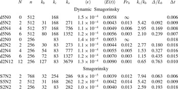
. Table 1 shows parameters and averaged quantities for the dynamic Smagorinsky LES in this paper, where
 $k_{o}=(N^{3}/{\it\epsilon})^{1/2}$
is based on
 $\langle {\it\epsilon}\rangle$
and
 $k_{b}$
is based on
 $u_{rms}$
.
List of numerical simulations.

As in Khani & Waite (Reference Khani and Waite2014), we consider the ability of the LES model to capture fundamental features of stratified turbulence at different resolutions. We have identified three features of stratified turbulence that are known to be suppressed in simulations when dissipation is too strong for a given stratification: an approximately
 $-5/3$
energy spectrum in the horizontal wavenumber; KH instabilities and billows on the stratified turbulence layers, with associated regions of small and negative Richardson number; and shallowing, or bumps, in the energy spectrum at the buoyancy scale, associated with the injection of energy from the KH instabilities. These characteristics have been found in many numerical studies of stratified turbulence, including DNS and hyperviscosity experiments: Lindborg (Reference Lindborg2006), Brethouwer et al. (Reference Brethouwer, Billant, Lindborg and Chomaz2007), Almalkie & de Bruyn Kops (Reference Almalkie and de Bruyn Kops2012) and Bartello & Tobias (Reference Bartello and Tobias2013) have found approximately
 $-5/3$
energy spectra; Laval et al. (Reference Laval, McWilliams and Dubrulle2003), Brethouwer et al. (Reference Brethouwer, Billant, Lindborg and Chomaz2007) and Waite (Reference Waite2011, Reference Waite, von Larcher and Williams2014) have discussed KH instabilities and associated bumps in the energy spectra. The recent high-resolution DNS by Bartello & Tobias (Reference Bartello and Tobias2013) also found KH instabilities and stratification-dependent bumps in the compensated energy spectra. These are not the only properties of stratified turbulence, but they are important, and they are clearly suppressed when dissipation is too strong; as a result, we have chosen to focus on these phenomena to identify a resolution criterion for LES. For LES with the Smagorinsky (Reference Smagorinsky1963) or Kraichnan (Reference Kraichnan1976) models, it seems only necessary that
 $L_{b}$
be sufficiently resolved (Khani & Waite Reference Khani and Waite2014).
4. Results and discussion
4.1. Buoyancy scale effects on the dynamic Smagorinsky model
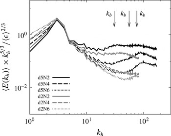
The compensated horizontal wavenumber energy spectra, in which the horizontal spectra are normalized by
 $k_{h}^{-5/3}\langle {\it\epsilon}\rangle ^{2/3}$
, are shown in figure 1. The advantage of using the compensated spectra is that constant horizontal spectra at intermediate wavenumbers imply a spectral slope of
 $-5/3$
, in line with the stratified turbulence inertial subrange theory of Lindborg (Reference Lindborg2006). The high-resolution case with
 $N=2$
shows an almost constant normalized spectrum over
 $6\lesssim k_{h}\lesssim 30$
along with a wide bump around
 $k_{b}\sim 30$
. The lower-resolution simulation with the same stratification exhibits a steeper spectrum, in which the bump around the buoyancy scale is weakly resolved. Increased stratification steepens the compensated horizontal wavenumber energy spectra, to the extent that the high-resolution cases with
 $N=4$
and 6 do not clearly show constant inertial subranges but resolve (small) bumps around
 $k_{b}\sim 60$
and 80, respectively. In addition, the low-resolution LES with larger stratification do not seem to capture any inertial subrange or bumps. In agreement with LES of stratified turbulence in Khani & Waite (Reference Khani and Waite2014), these results suggest that resolving a clear constant inertial subrange in the compensated horizontal wavenumber spectrum depends on the resolution and buoyancy frequency. As a result, stronger stratification may need higher resolution in LES to capture an inertial subrange.
The averaged compensated horizontal energy spectra. The spectra are averaged over
 $375\leqslant t\leqslant 450$
. From left to right, arrows show buoyancy wavenumbers
 $k_{b}$
that correspond to buoyancy frequencies
 $N=2$
, 4, and 6, respectively.

Khani & Waite (Reference Khani and Waite2014) have shown that in the Kraichnan and Smagorinsky LES, capturing dynamics of stratified turbulence depends on the ratio
 ${\it\Delta}/L_{b}$
. Only for sufficiently small values of
 ${\it\Delta}/L_{b}$
– below 0.47 for Kraichnan and 0.17 for Smagorinsky – were the small-scale features of stratified turbulence, including KH instabilities and locally small values of the Richardson number, captured. To evaluate the relevance of this criterion for the dynamic Smagorinsky model, we consider the horizontal vorticity fields as well as distributions of the local Richardson number in our stratified simulations.
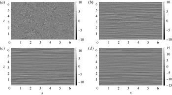
Figure 2 shows the
 $y$
component of vorticity
 $\bar{{\it\omega}}_{y}$
in the
 $x{-}z$
plane for the high-resolution simulations with different buoyancy frequencies at
 $y=0.25$
and
 $t=450$
. Unlike the unstratified case (figure 2
a), the stratified cases are layered in the vertical direction. KH instabilities are clearly visible in figure 2(b), but less so in figure 2(c,d); indeed, the increased stratification in figure 2(c,d) leads to decreasing numbers of KH billows. For stratified simulations, increased stratification inhibits KH instabilities as the layer thickness decreases towards the dissipation scale (e.g. Hebert & de Bruyn Kops Reference Hebert and de Bruyn Kops2006a
; Brethouwer et al.
Reference Brethouwer, Billant, Lindborg and Chomaz2007; Bartello & Tobias Reference Bartello and Tobias2013; Khani & Waite Reference Khani and Waite2014).
Vorticity field in the
 $y$
direction
 $\bar{{\it\omega}}_{y}$
on the
 $x{-}z$
plane at
 $y=0.25$
and
 $t=450$
for the high-resolution case with (a)
 $N=0$
, (b)
 $N=2$
, (c)
 $N=4$
, and (d)
 $N=6$
.

There is an apparent connection between cases with no inertial subrange in figure 1 and cases with no KH instabilities in figure 2. This connection has been noted previously in DNS (Waite Reference Waite, von Larcher and Williams2014) and other kinds of LES (Khani & Waite Reference Khani and Waite2014). To further investigate this connection with the dynamic Smagorinsky model, we consider the local Richardson number. The Richardson number shows the ratio of total (ambient plus perturbation) buoyancy frequency over the square of the vertical shears of horizontal motions, written as
 $$\begin{eqnarray}\mathit{Ri}=\frac{\displaystyle N^{2}-\frac{g}{{\it\rho}_{0}}\frac{\partial \bar{{\it\rho}}}{\partial z}}{\displaystyle \left(\frac{\partial \bar{u}}{\partial z}\right)^{2}+\left(\frac{\partial \bar{v}}{\partial z}\right)^{2}},\end{eqnarray}$$
where
 $N^{2}=-(g/{\it\rho}_{0})\partial {\it\Phi}_{0}/\partial z$
is constant,
 ${\it\rho}_{0}$
,
 $g$
and
 ${\it\Phi}_{0}$
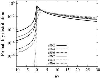
are the reference density, gravity and ambient density fields, respectively. Small Richardson numbers including negative values correspond to overturning and KH instabilities. Figure 3 shows the time-averaged histograms of the local Richardson number
 $\mathit{Ri}$
for the high- and low-resolution LES with different buoyancy frequencies. Histograms show long tails for positive
 $\mathit{Ri}$
and also rapid drops for negative
 $\mathit{Ri}$
. It appears that by increasing the resolution and decreasing buoyancy frequency, the peaks in the
 $\mathit{Ri}$
histograms move towards negative values, i.e. more of the domain is subject to KH and gravitational instabilities. In addition, the high-resolution case with
 $N=2$
(the solid black line) shows the largest number of points with negative values and the smallest number of points with positive
 $\mathit{Ri}$
. However, the low-resolution case with
 $N=6$
(the grey dotted line) shows the largest values for positive
 $\mathit{Ri}$
and just a few points with negative
 $\mathit{Ri}$
. Consistent with the Smagorinsky and Kraichnan LES of Khani & Waite (Reference Khani and Waite2014), increased resolution at fixed buoyancy frequency, or decreased stratification at fixed resolution, increases the number of points with small and negative
 $\mathit{Ri}$
. As a result, figure 3 demonstrates that increased resolution or decreased stratification are more likely to lead to generation of KH instabilities and overturning (consistent with the results of figure 2).
The averaged histograms of local Richardson number
 $\mathit{Ri}$
. Only the segment
 $-10\leqslant Ri\leqslant 30$
is shown. Histograms are normalized by bin size to give probability distributions, and are computed with 100 bins over the given segment (
 ${\rm\Delta}Ri=0.4$
).

Considering these findings, we can now attempt to find a threshold for
 ${\it\Delta}/L_{b}$
which guarantees that the breakdown of the layers into KH instabilities is captured (see Khani & Waite Reference Khani and Waite2014 for similar thresholds in the Kraichnan and Smagorinsky LES). According to table 1 and figure 3, if we consider cases with
 ${\it\Delta}<0.24L_{b}$
(i.e.
 $k_{c}>2.1k_{b}$
), the averaged
 $\mathit{Ri}$
histograms for
 $-10\leqslant Ri\leqslant 30$
are above
 $10^{-6}$
. On the other hand, if
 ${\it\Delta}>0.24L_{b}$
, only very few points with small and negative
 $\mathit{Ri}$
appear. These findings suggest that the maximum grid spacing for the dynamic Smagorinsky model should be in the range
 $0.18L_{b}<{\it\Delta}<0.24L_{b}$
. In contrast, the threshold for the regular Smagorinsky LES is in the range
 $0.12L_{b}\leqslant {\it\Delta}<0.17L_{b}$
(see Khani & Waite Reference Khani and Waite2014). While the dynamic Smagorinsky values are larger – i.e. lower resolution is able to capture the basic dynamics of stratified turbulence – these ranges nearly overlap, suggesting that the criteria for the regular and dynamic Smagorinsky are close. In the next section we compare these two SGS models and show that the dynamic Smagorinsky model is clearly better.
4.2. The dynamic Smagorinsky model versus the Smagorinsky model
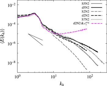
To get a better understanding of how well the dynamic Smagorinsky model performs in stratified turbulence simulations, we compare with results obtained with the regular Smagorinsky model at the same stratifications and resolutions (results from Khani & Waite Reference Khani and Waite2014; these simulations are labelled ‘S’ in table 1). Figure 4 shows the horizontal wavenumber energy spectra at different resolutions and fixed buoyancy frequency for both SGS models. Clearly, the dynamic version is less dissipative than the regular Smagorinsky model with the same resolution at large horizontal wavenumbers: at the same resolutions, the dynamic and regular Smagorinsky results agree fairly well at large scales but diverge at small scales, where the regular Smagorinsky results exhibit a much broader and steeper dissipation range. This is particularly pronounced at the lower resolution (
 $n=256$
), where the regular Smagorinsky spectrum is much steeper than the dynamic model over most wavenumbers. It is interesting that the dynamic case with
 $n=512$
is very similar to the Smagorinsky LES with
 $n=768$
; nevertheless, the Smagorinsky model is still more dissipative for
 $k_{h}\gtrsim 60$
. In addition, the low-resolution dynamic Smagorinsky case with
 $N=2$
is very close to the regular Smagorinsky LES with
 $n=512$
and
 $N=2$
. This trend implies that the dynamic Smagorinsky LES looks like the regular Smagorinsky case with twice the resolution. As a result, the low-resolution dynamic Smagorinsky model yields similar results to the high-resolution Smagorinsky model at fixed buoyancy frequency. It is worth mentioning that at the same resolution, both the dynamic and regular Smagorinsky models are almost identical at large scales: for the case with
 $n=256$
, they are very similar for
 $k_{h}<6$
, and for the case with
 $n=512$
, they are almost identical up to
 $k_{h}=20$
.
The averaged horizontal wavenumber energy spectra for the dynamic Smagorinsky cases compared with the Smagorinsky cases at different resolutions with fixed buoyancy frequency
 $N=2$
. The dot-dot-dashed (magenta online) curve shows the averaged horizontal wavenumber energy spectra over
 $300\leqslant t\leqslant 356$
for dynamic Smagorinsky simulation, in which
 $c_{s}$
values are space-averaged instead of clipping negative values. The solid black line segments show
 $-5/3$
and
 $-3$
slopes.

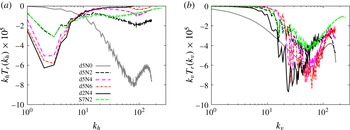
Figure 5 shows the horizontal and vertical wavenumber spectra of SGS energy transfer (i.e. eddy dissipation spectra) for stratified and unstratified dynamics models at
 $t=450$
. The eddy dissipation spectrum shows the rate of kinetic energy dissipation at resolved wavenumbers due to the eddy viscosity mechanism. In other words, the eddy dissipation spectra indicate the energy transfer from resolved scales towards the (unresolved) SGS motions. In order to compute the spectral SGS energy transfer, we multiply the Fourier coefficient of the eddy viscosity term in (2.1) with twice the complex conjugate of the Fourier coefficient of the filtered velocity field, and take the real part. For comparison, the eddy dissipation spectra of the Smagorinsky LES for the case with
 $n=768$
and
 $N=2$
(see Khani & Waite Reference Khani and Waite2014) are also shown. For unstratified cases, the maximum eddy dissipation occurs at small scales for both the horizontal and vertical wavenumber spectra. These trends are consistent with the isotropic dissipation picture, in which the kinetic energy is damped mainly at small scales. For stratified cases, however, the eddy dissipation spectra are very different in the horizontal and vertical directions. According to figure 5(a), the horizontal wavenumber spectra of SGS energy transfer peak at large scales.
The horizontal (a) and vertical (b) wavenumber spectra of SGS energy transfer for the low-resolution and high-resolution cases at
 $t=450$
. The spectra are multiplied by wavenumber in order to preserve area on the log-linear axes. For comparison, the results of high-resolution Smagorinsky LES are also shown (Khani & Waite Reference Khani and Waite2014).

Unlike the horizontal wavenumber spectra, the vertical wavenumber spectra of eddy dissipation for the stratified cases peak at small scales (figure 5
b). Increased stratification or decreased resolution increase the vertical SGS energy transfer spectra by contracting the thickness of vertical layers towards the dissipation scale or increasing dissipation scales, respectively (as seen in previous hyperviscosity simulations and DNS: Waite & Bartello Reference Waite and Bartello2004; Hebert & de Bruyn Kops Reference Hebert and de Bruyn Kops2006b
; Brethouwer et al.
Reference Brethouwer, Billant, Lindborg and Chomaz2007; Almalkie & de Bruyn Kops Reference Almalkie and de Bruyn Kops2012; Bartello & Tobias Reference Bartello and Tobias2013). As a result, for an isotropic eddy viscosity model, increased stratification leads to anisotropic eddy dissipation spectra due to strongly anisotropic resolved scales (see also Khani & Waite Reference Khani and Waite2014 for the Kraichnan and Smagorinsky models). It is worth mentioning that the horizontal and vertical eddy dissipation spectra of the dynamic Smagorinsky LES with
 $n=512$
and
 $N=2$
are very similar to their counterparts in the Smagorinsky LES with higher resolution
 $n=768$
and the corresponding buoyancy frequency, especially when
 $k_{h,v}\lesssim 60$
(figure 5). As a result, the low-resolution dynamic Smagorinsky model generates almost the same eddy dissipation as the high-resolution Smagorinsky model in LES of stratified turbulence. The results in figure 5 are consistent with the results of Khani & Waite (Reference Khani and Waite2013), who measured effective eddy viscosity and dissipation spectra in DNS of stratified turbulence. In particular, the maximum energy transfer from resolved scales towards SGS motions happens at large horizontal and small vertical scales (in line with the anisotropic dissipation in DNS of Khani & Waite Reference Khani and Waite2013).
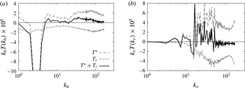
Figure 6 shows the horizontal and vertical energy transfer spectra for the stratified case with
 $n=512$
and
 $N=2$
at
 $t=450$
. The total kinetic energy transfer spectrum, which is shown by a solid black line in figure 6, is a summation of the resolved energy transfer spectrum
 $T^{\ast }$
plus the eddy dissipation spectrum
 $T_{r}$
. In the horizontal direction (figure 6
a), there is a large negative peak, which balances the energy input at large horizontal scales by the forcing term. In the intermediate range
 $7\lesssim k_{h}\lesssim 23$
, the energy transfer is approximately zero, which shows the stratified turbulence inertial subrange (Lindborg Reference Lindborg2006). At smaller resolved scales a positive bump around
 $k_{h}=30$
is seen, which indicates the injection of energy near the buoyancy scale
 $k_{b}$
, consistent with the development of KH instabilities and billows (in line with DNS and hyperviscosity simulations of Waite Reference Waite2011, Reference Waite, von Larcher and Williams2014). Figure 6(b) shows the vertical energy transfer spectrum, in which a peak around the buoyancy scale
 $k_{b}=30$
is observed, as in the horizontal. Overall, the transfer spectra seem broadly consistent with DNS results, which show transfer of energy out of the forcing scales and into the buoyancy scale (Almalkie & de Bruyn Kops Reference Almalkie and de Bruyn Kops2012; Waite Reference Waite, von Larcher and Williams2014).
The horizontal (a) and vertical (b) energy transfer spectra for the high-resolution stratified case with
 $N=2$
at
 $t=450$
. The spectra are multiplied by wavenumbers in order to preserve area on the log-linear axes. The thin black line shows the zero value.

In conclusion, this section shows that the maximum criterion on
 ${\it\Delta}/L_{b}$
for resolving KH instabilities in the dynamic Smagorinsky model is definitely larger than that for the regular Smagorinsky model. Even with half the resolution, the dynamic Smagorinsky model gives similar results to the regular Smagorinsky model (figure 4).
4.3. The dynamic Smagorinsky coefficient
 $c_{s}$

In this section, a detailed analysis on the dynamic Smagorinsky coefficient
 $c_{s}$
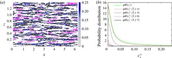
is presented. Figure 7(a) shows a snapshot for the
 $c_{s}^{+}$
field in the
 $x{-}z$
plane along with a few contours of the characteristic rate of strain
 $\bar{S}=(2\bar{\unicode[STIX]{x1D634}}_{ij}\bar{\unicode[STIX]{x1D634}}_{ij})^{1/2}$
at
 $y=0.25$
and
 $t=450$
for the high-resolution case with
 $N=4$
. The vertical axis is zoomed in to show around 13 vertical layers of length
 $2{\rm\pi}/k_{b}$
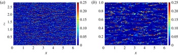
. It is interesting that the presence of stratification leads to vertical layers in the
 $c_{s}^{+}$
field. Black contours of
 $\bar{S}$
indicate low values
 $\bar{S}=1$
and 1.5. The magenta contours on the other hand show higher values
 $\bar{S}=6$
and 8. Interestingly, regions with high straining in figure 7 are generally associated with zero or very small values of
 $c_{s}^{+}$
, while regions with low straining correspond to larger values of
 $c_{s}^{+}$
. This behaviour, which has been investigated elsewhere in unstratified turbulence (e.g. Kleissl et al.
Reference Kleissl, Kumar, Meneveau and Parlange2006; Wan & Porté-Agel Reference Wan and Porté-Agel2011), suggests that the dynamic Smagorinsky coefficient
 $c_{s}$
decreases as shear increases in order to preserve the small-scale instabilities between vertical layers.
(a) The Smagorinsky coefficient field
 $c_{s}^{+}$
on the
 $x{-}z$
plane and (b) the conditional distribution of
 $c_{s}^{+}$
, for the high-resolution case with
 $N=4$
at
 $y=0.25$
and
 $t=450$
. In (a), contours of constant
 $\bar{S}=(2\bar{\unicode[STIX]{x1D634}}_{ij}\bar{\unicode[STIX]{x1D634}}_{ij})^{1/2}$
are overlaid on the
 $c_{s}^{+}$
field where the vertical axis is zoomed in to
 $80/k_{b}$
that includes around
 $13L_{b}$
. The magenta contours present high values
 $\bar{S}=6$
and 8 and the black contours show those of low values
 $\bar{S}=1$
and 1.5.

Figure 7(b) shows the probability distributions of
 $c_{s}^{+}$
on gridpoints restricted to different ranges of
 $\bar{S}$
at
 $t=450$
. It is clear that increased straining is associated with smaller values of
 $c_{s}^{+}$
. With weak straining, distributions of the dynamic Smagorinsky coefficient
 $c_{s}^{+}$
show both small and large
 $c_{s}^{+}$
values. However, for large straining, these distributions show small
 $c_{s}^{+}$
values. For example, for
 $\bar{S}\geqslant 7$
, the solid black line in figure 7(b),
 $c_{s}^{+}$
values are smaller than
 $(0.14)^{2}$
. This trend is consistent with the suggestion of Deardorff (Reference Deardorff1971) that the presence of shear implies small
 $c_{s}^{+}$
values. In addition, looking at
 $c_{s}^{+}$
fields at different stratifications shows that increased stratification at fixed resolution leads to vertical layers that are not fully resolved, consistent with failure of the criterion on
 ${\it\Delta}/L_{b}$
(see figure 8).
The Smagorinsky coefficient field
 $c_{s}^{+}$
on the
 $x{-}z$
plane for the high-resolution cases with (a)
 $N=2$
and (b)
 $N=6$
at
 $y=0.25$
and
 $t=450$
, where the vertical axes are zoomed in to
 $80/k_{b}$
to include around
 $13L_{b}$
.

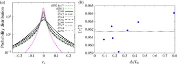
The time-averaged histograms of
 $c_{s}$
at different resolutions and buoyancy frequencies are shown in figure 9(a). Increased stratification leads to decreasing standard deviations, i.e.
 $c_{s}$
values tend to get smaller (consistent with figure 7). Interestingly, the distribution of negative
 $c_{s}$
(before clipping is applied) is very similar to that of positive
 $c_{s}$
; similar trends are seen in Kang, Chester & Meneveau (Reference Kang, Chester and Meneveau2003), Meneveau, Lund & Cabot (Reference Meneveau, Lund and Cabot1996) for probability distributions of local SGS dissipation, and probability distributions of
 $c_{s}$
, respectively. As discussed in § 2, negative
 $c_{s}$
values occur when the resolved stress
 $\unicode[STIX]{x1D613}_{ij}$
and Germano’s rate of strain
 $\unicode[STIX]{x1D614}_{ij}$
are not coaxial, implying backscatter. Since we remove negative
 $c_{s}$
values at every time step to prevent numerical instabilities, the clipping procedure removes some local information about the modelled SGS stress tensor and the dynamics of upscale energy transfer, which are not appropriately represented with an eddy viscosity model. In addition, this plot shows that the volume-averaged
 $c_{s}$
values are very close to zero. Figure 9(b) shows the time-and-space average (denoted by double angle brackets
 $\langle \langle \cdot \rangle \rangle$
) of
 $c_{s}^{+}$
versus
 ${\it\Delta}/L_{b}$
. It is interesting that the time- and space-averaged
 $c_{s}^{+}$
for stratified cases is around
 $\langle \langle c_{s}^{+}\rangle \rangle =(0.25)^{2}$
(the dashed black line in figure 9
b), which is only slightly larger than that of the non-stratified case with
 $\langle \langle c_{s}^{+}\rangle \rangle =(0.23)^{2}$
, and also larger than the regular Smagorinsky constant
 $c_{s}=(0.17)^{2}$
. This behaviour might suggest that the presence of stratification decreases straining in turbulent flows and so the dynamic Smagorinsky model implies larger
 $c_{s}$
in stratified turbulence, corresponding to changes in dynamics of flows as stratification appears (see also figure 7). Interestingly, the probability distributions of
 $c_{s}$
in stratified turbulence are symmetric, which is not the case for
 $c_{s}^{+}$
(in line with the isotropic turbulence: Meneveau et al.
Reference Meneveau, Lund and Cabot1996; Kang et al.
Reference Kang, Chester and Meneveau2003).
(a) The averaged histograms of Smagorinsky coefficient
 $c_{s}$
and (b) the time- and space-averaged
 $c_{s}$
versus
 ${\it\Delta}/L_{b}$
. In (a), only the segment
 $-0.25\leqslant c_{s}\leqslant 0.25$
is shown. Histograms are normalized by bin size to give probability distributions, and are computed with 100 bins over the given segment (
 ${\rm\Delta}c_{s}=0.005$
). The dashed line in (b) shows the average of all
 $\langle \langle c_{s}^{+}\rangle \rangle$
values.

It is interesting that the self-similar assumption of the dynamic Smagorinsky model works reasonably well in stratified turbulence when
 ${\it\Delta}\sim L_{b}$
. A possible explanation for this behaviour could be the development and breakdown of KH billows, which are much more isotropic than the larger-scale layerwise structures. In addition, DNS results of stratified turbulence show that the effective spectral eddy viscosity has self-similar structure when the test cutoff
 $k_{c}$
is around
 $k_{o}$
or smaller (Khani & Waite Reference Khani and Waite2013).
An alternative to clipping negative
 $c_{s}$
values is to use spatial averaging of
 $c_{s}$
over the homogeneous directions, as is often done in boundary layer simulations (e.g. Meneveau & Katz Reference Meneveau and Katz2000; Pope Reference Pope2000; Porté-Agel et al.
Reference Porté-Agel, Meneveau and Parlange2000). Here, since we are considering homogeneous stratified turbulence, this approach amounts to taking a spatial average of
 $c_{s}$
before evaluating the eddy viscosity (1.2). We have evaluated this approach by performing an additional simulation with
 $n=256$
and
 $N=2$
, in which
 $c_{s}$
values are averaged over the entire domain instead of clipping negative
 $c_{s}$
values. Because of the lack of sufficient dissipation at small scales, the simulation in this case blew up at around
 $t=356$
(see the dot-dot-dashed (magenta online) curve in figure 4, which clearly shows an artificial pile-up of energy at large wavenumbers). The averaged probability distribution of
 $c_{s}$
for this simulation over
 $300\leqslant t\leqslant 356$
is also shown in figure 9(a), in which shorter tails and a larger peak are seen. For this case, the standard deviation is half of that seen when clipping negative
 $c_{s}$
values.
5. Conclusions
A systematic analysis of the performance of the dynamic Smagorinsky model in stratified turbulence has been studied in this paper. Our results show that if
 ${\it\Delta}/L_{b}<0.24$
, several key features of stratified turbulence – including an energy spectrum with an approximately
 $-5/3$
slope in the horizontal, KH instabilities and overturning – are captured in LES of stratified turbulence using the dynamic Smagorinsky model. Other SGS models have different criteria for
 ${\it\Delta}/L_{b}$
. For example, Khani & Waite (Reference Khani and Waite2014) argued that for the Smagorinsky and Kraichnan model
 ${\it\Delta}/L_{b}$
should be less than 0.17 and 0.47, respectively, to ensure these features of stratified turbulence are captured. As a result, the resolution limit on
 ${\it\Delta}$
in the dynamic Smagorinsky model is 40 % larger than that of the Smagorinsky model (see figure 4). In addition, this study shows that spectra of SGS energy transfers in stratified simulations are significantly different in the horizontal and vertical directions, in line with other LES models (Khani & Waite Reference Khani and Waite2014). The maximum eddy dissipation spectra in stratified cases occur at large horizontal and small vertical scales. This behaviour suggests that spectra of SGS energy transfer are anisotropic in stratified turbulence. Overall, the eddy dissipation from the dynamic Smagorinsky LES with
 $N=2$
and
 $n=512$
looks similar to the regular Smagorinsky LES at the same buoyancy frequency with
 $n=768$
.
The dynamic eddy viscosity coefficient
 $c_{s}^{+}$
shows a layerwise field in the presence of stratification, consistent with the familiar layered structure of stratified turbulence. This finding implies that the dynamic Smagorinsky model can make a connection between the SGS model and stratification and that this connection yields an improvement on the performance of traditional SGS models like the Smagorinsky model in stratified turbulence. It is interesting that large values of
 $c_{s}^{+}$
correspond to regions with weak straining. Consistently, in regions with large shears (strong vertical straining), the values of
 $c_{s}^{+}$
are very small. This behaviour explains why the dynamic Smagorinsky model is overall less dissipative than the regular Smagorinsky model. Also, the overall relationship between
 $c_{s}^{+}$
and shear
 $\bar{S}$
is similar to what has been discussed in the literature on unstratified turbulence. In addition, local distributions of negative
 $c_{s}$
are very close to positive
 $c_{s}$
, implying that local negative dissipation (i.e. backscatter) might be important in the dynamic Smagorinsky model. Nevertheless, negative values of
 $c_{s}$
are set to zero in this study to stabilize the simulations and ensure sufficient small-scale dissipation. Ultimately, the appropriate inclusion of backscatter in LES requires a different approach from the eddy viscosity model (e.g. Carati, Ghosal & Moin Reference Carati, Ghosal and Moin1995; Ghosal et al.
Reference Ghosal, Lund, Moin and Akselvoll1995).
At the same resolution, the dynamic Smagorinsky model is much more expensive than the regular Smagorinsky model; wall clock run times are approximately twice as long. This increase in run time is due to the significant increase in the number of fast Fourier transforms (FFTs) required to compute
 $c_{s}$
. On the other hand, the dynamic Smagorinsky model can be run at lower resolution and still give similar results to the regular Smagorinsky model. Decreasing the resolution by 33 % (i.e. from
 $n=768$
to
 $n=512$
) cuts the run time by a factor of 5. Halving the resolution (i.e. from
 $n=512$
to
 $n=256$
) cuts the run time by a factor of 16, and still gives dynamic Smagorinsky results similar to regular Smagorinsky. Despite the increased number of FFTs, the ability to run at lower resolution implies that the dynamic Smagorinsky approach is clearly more efficient than the regular Smagorinsky method.
Overall, we have now looked at three SGS models: Kraichnan, Smagorinsky and dynamic Smagorinsky. Despite the fact that these models were designed for unstratified turbulence, they work well for stratified turbulence when
 $L_{b}$
is resolved sufficiently. The interpretation of ‘sufficiently’ depends on the model. The Kraichnan model is clearly the best – i.e. it requires the lowest resolution to give the same results – but it only works for triply periodic spectral models. Otherwise, the dynamic Smagorinsky model is better than regular Smagorinsky. However, none of these models work well when
 $L_{b}$
is not resolved. Eliminating this barrier, i.e. running LES without fully resolving
 $L_{b}$
, would require a major rework. For future work, performing LES of stratified turbulence with anisotropic eddy viscosity terms could be considered. In addition, considering local backscatter in the dynamic SGS models is another potential avenue in studying of stratified turbulence. Ultimately, we need to perform a high-resolution DNS of stratified turbulence to study the dynamics of energy transfer around the buoyancy scale
 $L_{b}$
and maybe the Ozmidov scale
 $L_{o}$
.
Acknowledgements
Computations were performed on the GPC supercomputer at the SciNet HPC Consortium. SciNet is funded by the Canada Foundation for Innovation under the auspices of Compute Canada, the Government of Ontario, Ontario Research Fund – Research Excellence, and the University of Toronto. Also, this work was made possible by the facilities of the Shared Hierarchical Academic Research Computing Network (SHARCNET: www.sharcnet.ca) and Compute/Calcul Canada. Financial support from the Natural Sciences and Engineering Research Council of Canada is gratefully acknowledged.