1 Introduction
The mixing and transport dynamics of flow through ordered porous structures is fundamental to many man-made and natural processes, ranging from nano/micro-fluidics (deMello Reference deMello2006), chromatography (Fair & Kormos Reference Fair and Kormos2008) and macroscopic fluid processing (Meijer, Singh & Anderson Reference Meijer, Singh and Anderson2012), through to studies of dilution in structured granular media (Ye et al. Reference Ye, Chiogna, Cirpka, Grathwohl and Rolle2015). The virtually unlimited design flexibility of new manufacturing technologies (e.g. three-dimensional printing) opens the door to the development of structured materials with tuneable transport properties. Whilst this relationship has been exploited to design e.g. static mixers (Meijer et al. Reference Meijer, Singh and Anderson2012) and catalyst supports (Avril et al. Reference Avril, Hornung, Urban, Fraser, Horne, Veder, Tsanaktsidis, Rodopoulos, Henry and Gunasegaram2017), a systematic understanding of how the basic crystal structure controls mixing and dispersion is an outstanding problem.
In the context of natural porous media, mixing mechanisms at the pore scale have also been under intense scrutiny following observations that classical transport models assuming well-mixed conditions at scales below the continuum/Darcy scale fail to predict the dynamics of mixing-mediated chemical reactions (Tartakovsky, Tartakovsky & Meakin Reference Tartakovsky, Tartakovsky and Meakin2008; Battiato et al. Reference Battiato, Tartakovsky, Tartakovsky and Scheibe2009; Dentz et al. Reference Dentz, LeBorgne, Englert and Bijeljic2011; De Anna et al. Reference De Anna, Jimenez-Martinez, Tabuteau, Turuban, Borgne, Derrien and Meheust2014). Despite recent investigations of pore-scale velocity distributions and their impact on solute transport (Bijeljic, Mostaghimi & Blunt Reference Bijeljic, Mostaghimi and Blunt2011; Kang et al. Reference Kang, Anna, Nunes, Bijeljic, Blunt and Juanes2014; Holzner et al. Reference Holzner, Morales, Willmann and Dentz2015), the link between pore-scale complexity and mixing dynamics still remains an open question.
In these studies the term ‘mixing’ refers to the physical process of dilution of a diffusive scalar (i.e. a solute specie) which results in the reduction of concentration variance under the combined actions of advection and diffusion; this is the conventional definition of mixing. However, the term ‘mixing’ is also used in fluid mechanics in the context of dynamical systems, to refer to the ergodicity of the trajectories of diffusionless particles due to advection alone (Ottino Reference Ottino1989). This ergodic mixing relates to the Lagrangian kinematics of the flow and is concerned with the geometry of particle trajectories rather than the evolution of a solute plume. It is important to note that these two different physical concepts denoted as ‘mixing’ are linked, as conventional mixing and dilution results from the interplay of molecular diffusion and ergodic mixing; thus it is impossible to fully understand physical mixing without insight into the underlying Lagrangian kinematics. In this study we address ergodic mixing in three-dimensional (3-D) porous media.
Recent studies of ergodic mixing in 3-D porous media involving a continuous (i.e. not granular) solid phase have shown that randomly oriented fluid stretching at stagnation points local to pore junctions generates chaotic mixing (Lester, Metcalfe & Trefry Reference Lester, Metcalfe and Trefry2013; Lester, Dentz & Le Borgne Reference Lester, Dentz and Le Borgne2016b ) (otherwise known as Lagrangian chaos or Lagrangian turbulence, defined as the persistent, exponential elongation of fluid elements in time) under steady flow conditions. However, it was unknown whether these concepts extend to the large class of discrete (i.e. granular) 3-D porous media. The topological complexity of these materials depends on grain contacts of zero measure, and therefore differs significantly from that of continuous 3-D porous media. Pore networks also constrain fluid flow to a greater extent than granular media, hence fluid stretching and folding – the hallmarks of chaotic advection – are more likely in the former. As reflected by the minimum energy dissipation theorem (Kim & Karrila Reference Kim and Karrila1991), these deformations are typically unfavourable in steady Stokes flow.
In this study we investigate the mechanisms of chaotic fluid mixing in granular media. For that purpose, we examine the Lagrangian kinematics of non-diffusive fluid particles through granular lattices comprised of crystalline close-packed spheres; the impacts of these kinematics upon diffusive mixing shall be considered in subsequent studies. Owing to the
 $SO(3)$
rotational symmetry of the spherical grains, the mixing dynamics is entirely controlled by the structure of the granular lattice and mean flow orientation with respect to that lattice. As such, orientation of the mean flow with respect to the symmetries of the granular lattice plays a key role in organising the Lagrangian kinematics. It is well known that symmetry breaking is often a necessary condition for Lagrangian chaos to occur (Mezić & Wiggins Reference Mezić and Wiggins1994; Haller & Mezic Reference Haller and Mezic1998; Yannacopoulos et al.
Reference Yannacopoulos, Mezić, Rowlands and King1998; Franjione, Leong & Ottino Reference Franjione, Leong and Ottino1989). Hence chaotic mixing (and hydrodynamic dispersion) cannot occur when the mean flow direction is aligned normal to the reflection symmetries of the granular lattice due to the reversibility of Stokes flow. In addition to the above well-established behaviour regarding symmetry breaking, we have recently (Turuban et al.
Reference Turuban, Lester, Borgne and Méheust2018) uncovered the surprising result that other types of symmetries can play a direct role in the generation of Lagrangian chaos. The key difference is that whilst breaking of e.g. reflection symmetries which belong to the point group symmetries of the granular lattice are necessary for Lagrangian chaos, the presence of space group symmetries (e.g. involving combined translation and reflection) can generate chaotic mixing. Turuban et al. (Reference Turuban, Lester, Borgne and Méheust2018) show that the body-centered cubic (BCC) and simple cubic (SC) lattices exhibit significantly different Lagrangian kinematics despite sharing the same point group, due to the fact that they possess different space groups.
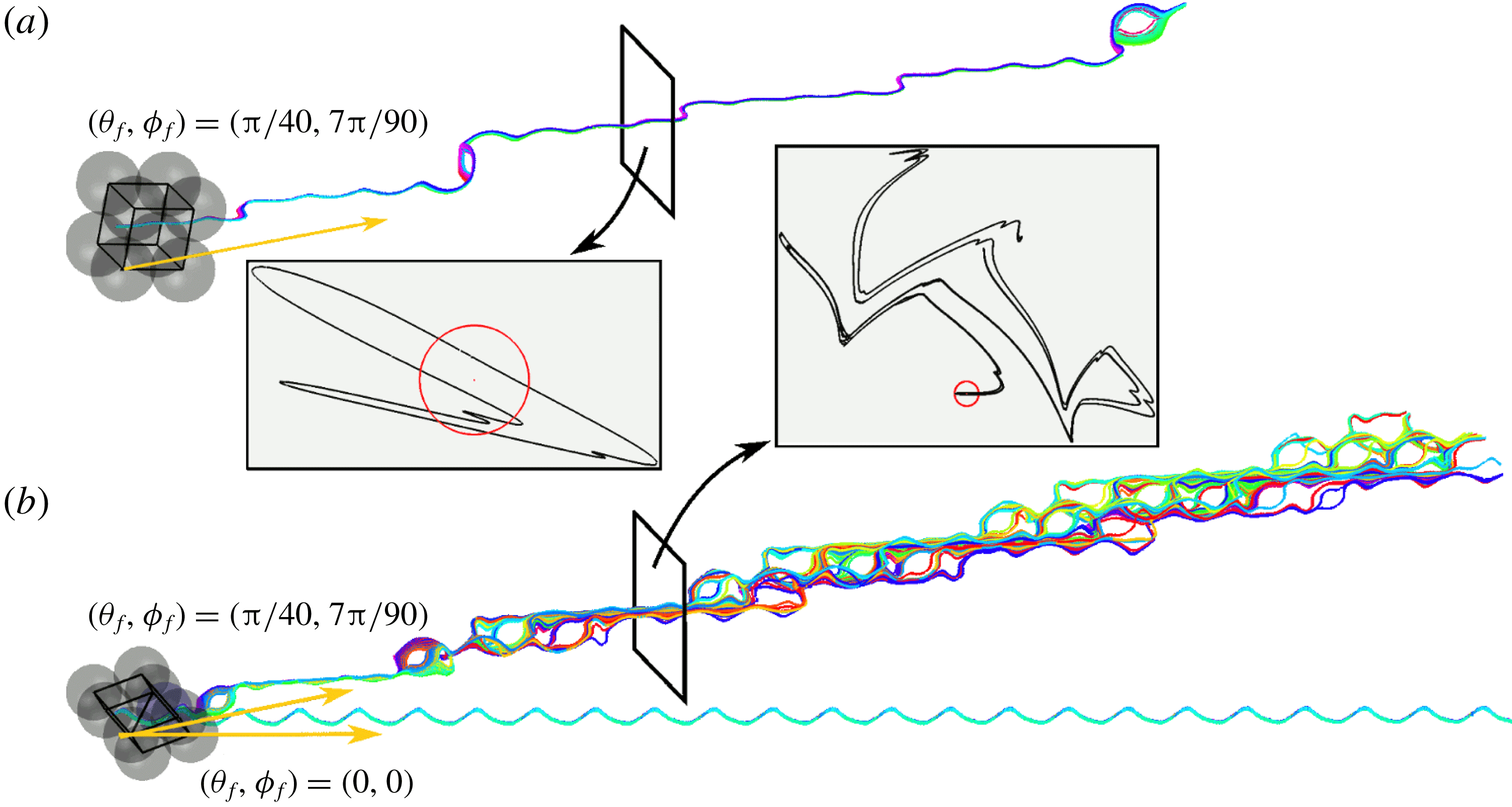
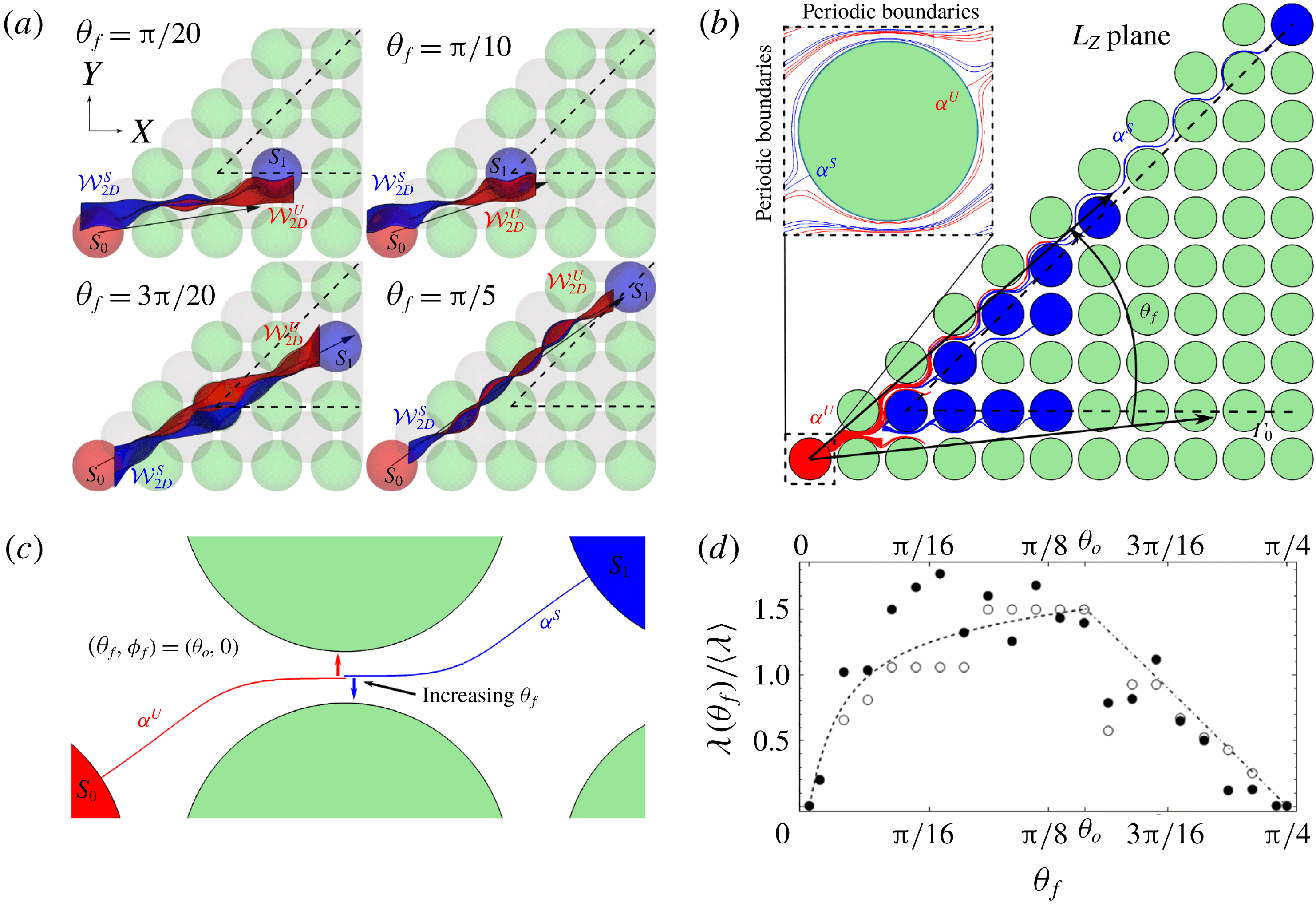
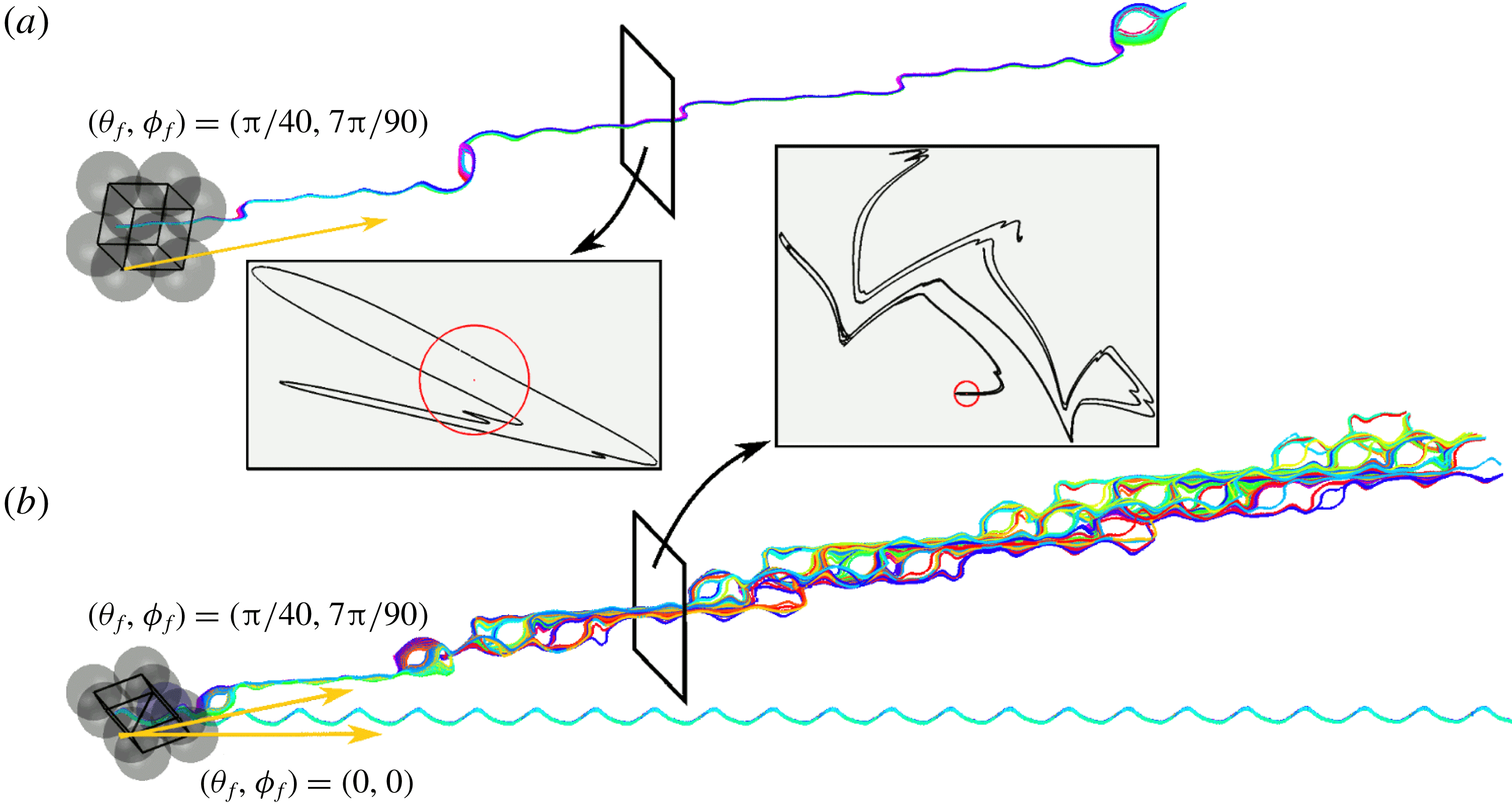
This behaviour is illustrated in figure 1, which shows the evolution of particle trajectories in the SC and BCC packings for various mean flow orientations
 $(\unicode[STIX]{x1D703}_{f},\unicode[STIX]{x1D719}_{f})$
relative to the lattice axes. As expected, for flows perpendicular to reflection symmetries of the crystalline sphere lattice (e.g.
 $(\unicode[STIX]{x1D703}_{f},\unicode[STIX]{x1D719}_{f})=(0,0)$
in figure 1), we observe completely integrable (i.e. non-chaotic) transport with zero net transverse hydrodynamic dispersion. Conversely, under weak symmetry breaking (e.g.
 $(\unicode[STIX]{x1D703}_{f},\unicode[STIX]{x1D719}_{f})=(\unicode[STIX]{x03C0}/40,7\unicode[STIX]{x03C0}/90)$
), chaotic mixing and transverse hydrodynamic dispersion are observed in both the BC and SCC lattices. Furthermore, for the same flow orientation, the BCC lattice is observed to impart much stronger mixing than the SC lattice, which stems from the presence of space group symmetries in the BCC lattice (Turuban et al.
Reference Turuban, Lester, Borgne and Méheust2018). This stronger mixing is visible when comparing the two insets in figure 1, and can be assessed quantitatively from the corresponding Lyapunov exponents (see figure 3), which are defined as the rate of exponential stretching of fluid elements and are commonly used as a qualitative measure for the rate of mixing.
These results have significant implications for both local fluid mixing and the upscaling of transport and dispersion in ordered porous media. Transverse and longitudinal macro-dispersion is governed by the interplay between the geometry of fluid streamlines and molecular diffusion (Lester, Trefry & Metcalfe Reference Lester, Trefry and Metcalfe2016a ; Lester et al. Reference Lester, Dentz and Le Borgne2016b ), and so the different behaviours exhibited in figure 1(a,b) can lead to very different macroscopic phenomena. Here, chaotic trajectories directly retard longitudinal dispersion via an accelerated Taylor–Aris mechanism Jones & Young (Reference Jones and Young1994), Mezić, Wiggins & Bentz (Reference Mezić, Wiggins and Bentz1999), Lester, Metcalfe & Trefry (Reference Lester, Metcalfe and Trefry2014) (as space-filling, chaotic fluid trajectories evenly sample all of the velocity distribution), and (as shown in figure 1 b), chaotic trajectories provide a mechanism for transverse hydrodynamic dispersion in steady flows (Lester et al. Reference Lester, Trefry and Metcalfe2016a ,Reference Lester, Dentz and Le Borgne b ). Whilst the study and quantification of these phenomena is beyond the scope of this study, we shall address their implications in future work.
(a) Particle trajectories for the flow orientation
 $(\unicode[STIX]{x1D703}_{f},\unicode[STIX]{x1D719}_{f})=(\unicode[STIX]{x03C0}/40,7\unicode[STIX]{x03C0}/90)$
in the SC lattice. Inset: cross-section (black line) of a material surface resulting from the continuous injection of material line (light grey (red online) circle) 12.5 sphere diameters upstream. (b) Particle trajectories for two flow orientations in the BCC lattice:
 $(\unicode[STIX]{x1D703}_{f},\unicode[STIX]{x1D719}_{f})=(0,0)$
,
 $(\unicode[STIX]{x03C0}/40,7\unicode[STIX]{x03C0}/90)$
, illustrating a sharp transition from regular flow to strong chaotic mixing under weak perturbation of the flow orientation. Inset: same as for (a) for the latter orientation, also see supplementary movie 1 available at https://doi.org/10.1017/jfm.2019.245. Adapted from Turuban et al. (Reference Turuban, Lester, Borgne and Méheust2018).
In this study we extend the analysis of Turuban et al. (Reference Turuban, Lester, Borgne and Méheust2018) to investigate topological constraints which explain the fundamental differences between Lagrangian chaos in continuous and discrete porous media. This requires unpacking some of the material in Turuban et al. (Reference Turuban, Lester, Borgne and Méheust2018) in much greater detail to develop insights into the mechanisms that govern chaotic mixing in granular porous media. We then utilise these insights to develop quantitative predictions of Lagrangian kinematics over the parameter space of mean flow orientations
 $(\unicode[STIX]{x1D703}_{f},\unicode[STIX]{x1D719}_{f})$
relative to the crystalline axes. We start by defining the sphere lattices (§ 2) and exploring their underlying symmetries, then briefly review the mechanisms of chaotic mixing in discrete porous media (§ 3). In § 4 we consider the implications of singular contacts between grains and underlying symmetries of the sphere lattices upon these mechanisms. These insights are then used in § 5 to develop a predictive model of the dependence of the Lyapunov exponent on the flow orientation with respect to the crystalline axes of the sphere lattices.
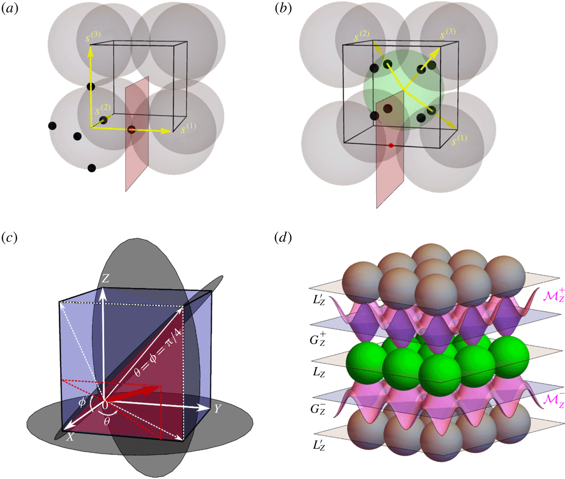
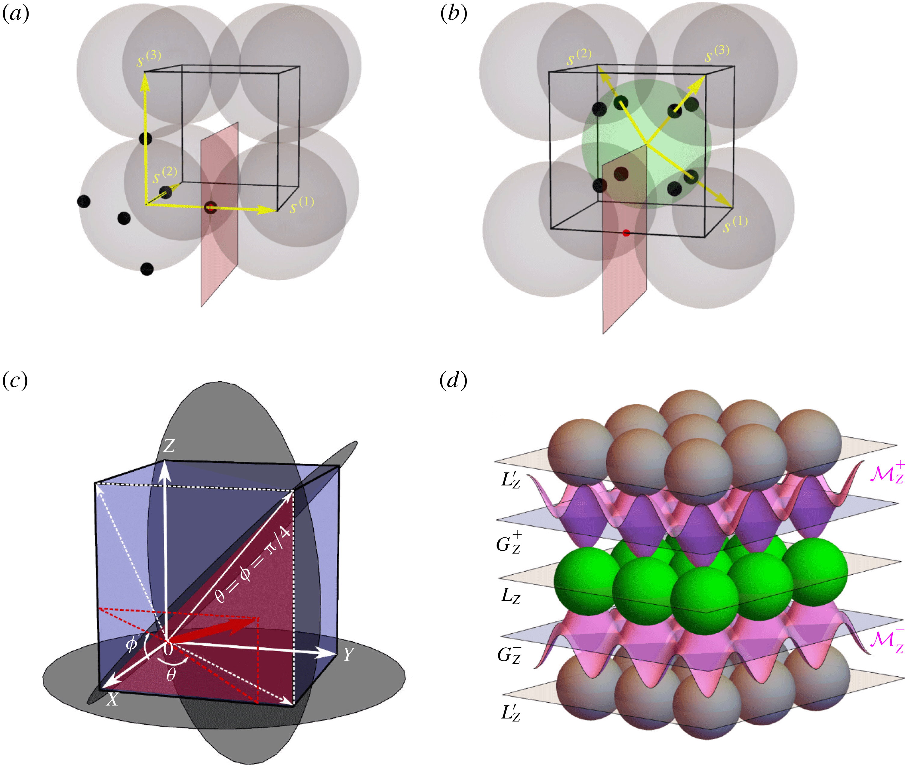
Cubic unit cell (black) for the (a) SC and (b) BCC packings, basis vectors (yellow)
 $\boldsymbol{s}^{1}$
,
 $\boldsymbol{s}^{2}$
and
 $\boldsymbol{s}^{3}$
define the corresponding primitive cell. Black dots denote the contact points between the spheres, for one single sphere. Grey (red online) planes correspond to the Poincaré sections in figure 5. Their intersection with one of the edges of the cubic unit cell is indicated by a grey (red online) point; for SC it coincides with a contact point. (c) (
 $\unicode[STIX]{x1D703}_{f},\unicode[STIX]{x1D719}_{f}$
) coordinate system for the mean flow orientation
 $\boldsymbol{q}$
, along with selected reflection symmetry planes (grey discs) of the SC/BCC unit cells
 $S_{2}^{m}=[1,-1,0]$
,
 $[0,0,1]$
,
 $[0,1,-1]$
. These symmetry planes reduce the unique flow orientations to the parameter space
 ${\mathcal{H}}:(\unicode[STIX]{x1D719},\unicode[STIX]{x1D703})=[0,\unicode[STIX]{x03C0}/4]\times [0,\unicode[STIX]{x03C0}/4]$
, as indicated by the dark grey (magenta online) region. (d) Vertically exploded view of sphere layers (where spheres in the
 $L_{Z}$
and
 $L_{Z}^{\prime }$
planes are coloured light grey (green online) and grey, respectively) in the BCC lattice for
 $\unicode[STIX]{x1D719}_{f}=0$
. Here
 $L_{Z}$
,
 $L_{Z}^{\prime }$
denote the reflection and
 $G_{Z}^{\pm }$
glide symmetry planes and
 ${\mathcal{M}}_{Z}^{\pm }$
are the associated material surfaces (light grey, pink online). Adapted from Turuban et al. (Reference Turuban, Lester, Borgne and Méheust2018).
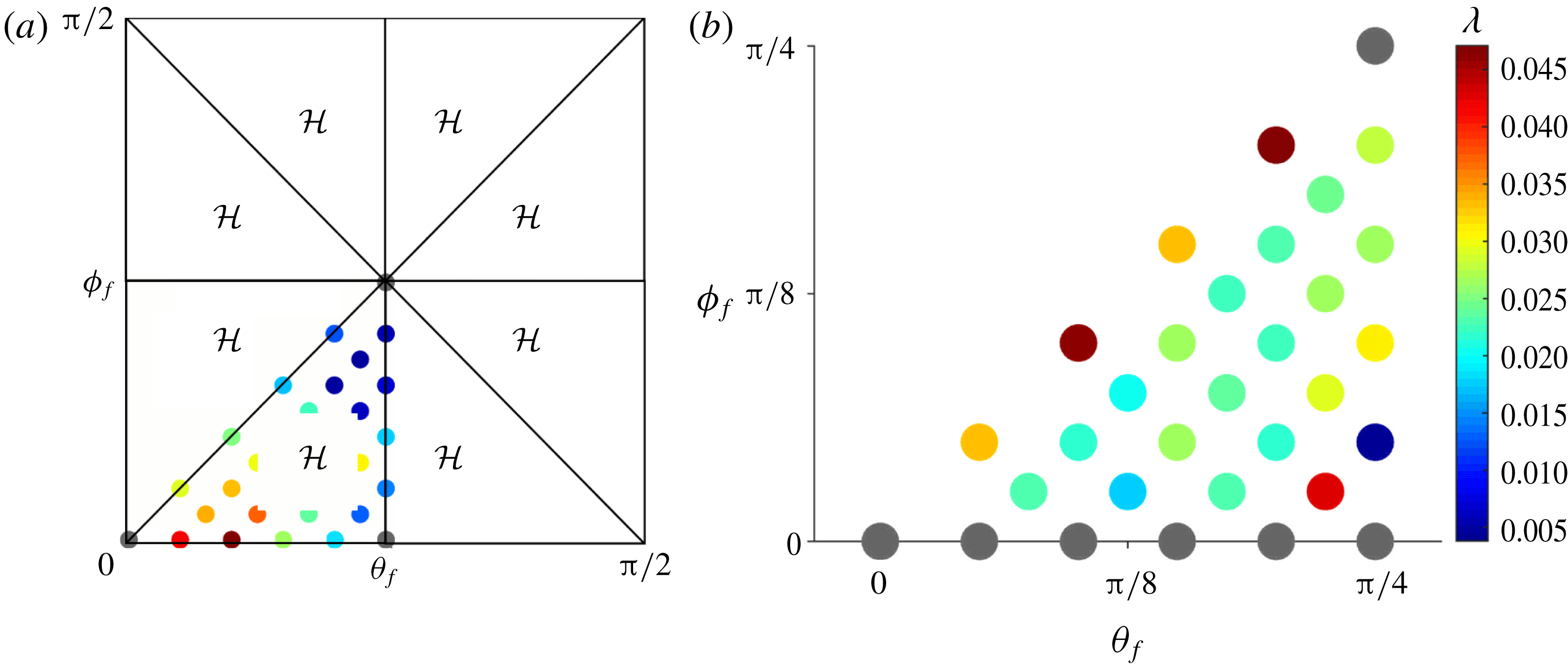
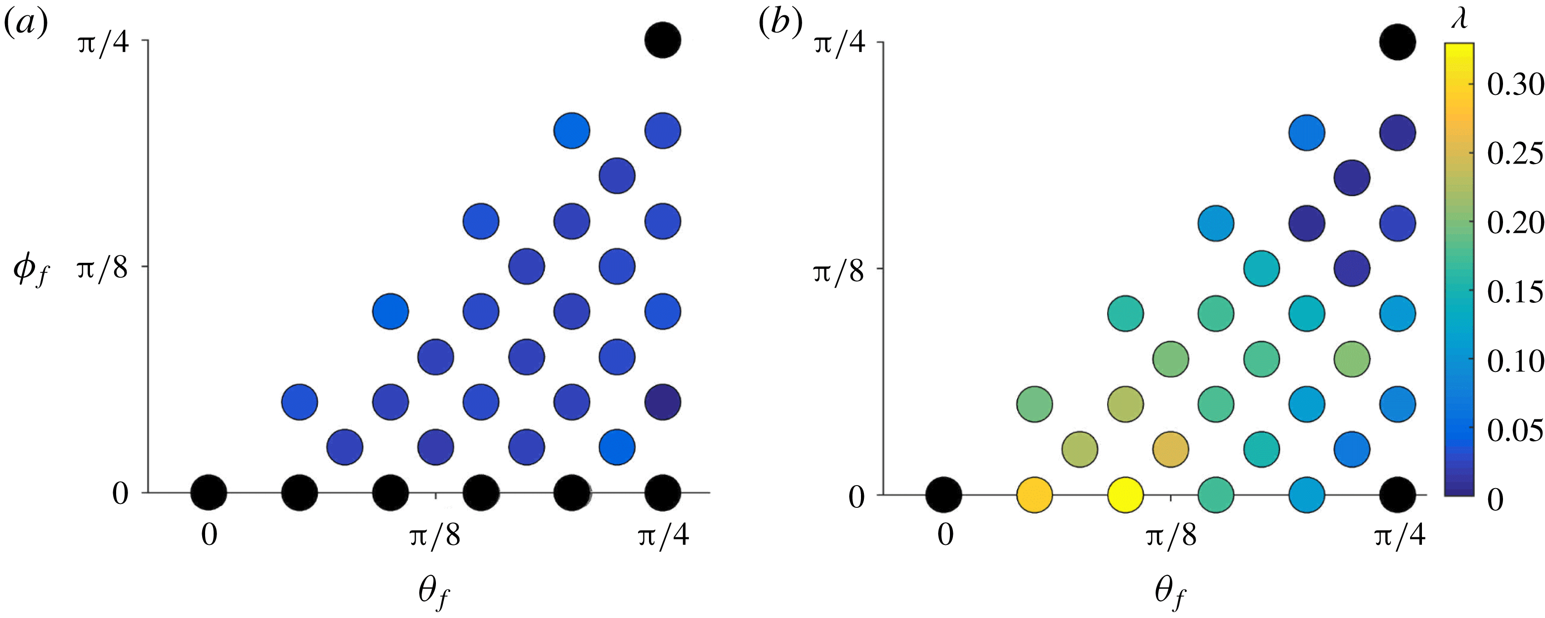
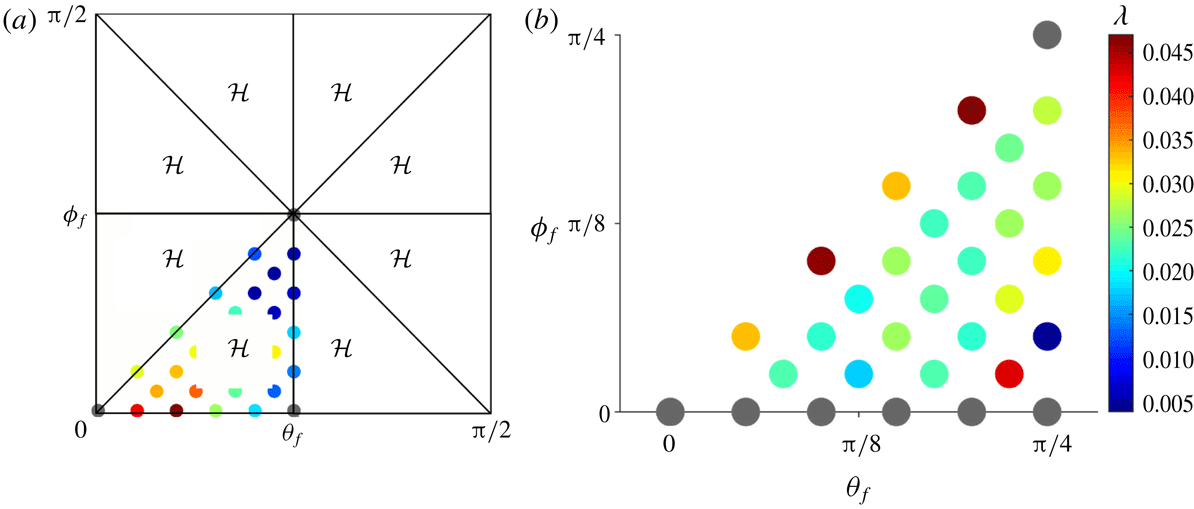
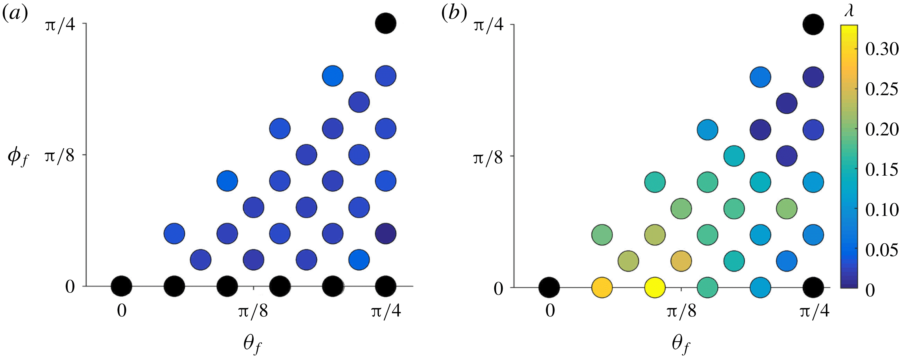
Distribution of the Lyapunov exponent
 $\unicode[STIX]{x1D706}$
over the parameter space
 ${\mathcal{H}}$
for (a) SC and (b) BCC packings. Note that black denotes globally regular Lagrangian dynamics (i.e.
 $\unicode[STIX]{x1D706}=0$
), which arises due to alignment of the mean flow normal to a reflection symmetry
 $S_{m}^{i}$
. Adapted from Turuban et al. (Reference Turuban, Lester, Borgne and Méheust2018). A version of (a) with a different colour scale is shown in figure 15 to more clearly illustrate the Lyapunov exponent distribution over the parameter space
 ${\mathcal{H}}$
for the SC packing.
2 Sphere lattice symmetries and impact upon Lagrangian chaos
2.1 Symmetries of SC and BCC sphere lattices
The simple cubic (SC) and body-centred cubic (BCC) sphere arrays consist of lattices of uniform, close-packed unit radius spheres, as illustrated by their cubic unit cells in figure 2(a,b). These lattices are defined in the 3-D space
 $\unicode[STIX]{x1D6FA}:[X,Y,Z]=(-\infty ,\infty )\times (-\infty ,\infty )\times (-\infty ,\infty )$
in terms of the base vectors
 $\boldsymbol{s}^{(i)}$
, where the sphere centres are positioned at
 $$\begin{eqnarray}\displaystyle \boldsymbol{r}=\boldsymbol{r}_{0}+n_{1}\boldsymbol{s}^{(1)}+n_{2}\boldsymbol{s}^{(2)}+n_{3}\boldsymbol{s}^{(3)}, & & \displaystyle\end{eqnarray}$$
with integers
 $n_{i}=0$
,
 $\pm 1$
,
 $\pm 2$
,
 $\ldots \,$
. Here
 $\boldsymbol{r}_{0}=(-\ell /2,-\ell /2,-\ell /2)$
is such that the unit cell corresponding to
 $(n_{1},n_{2},n_{3})=(0,0,0)$
is centred at the origin, and
 $\ell$
is the length of the lattice unit cell. The base vectors for the SC and BCC lattices are respectively
 $$\begin{eqnarray}\displaystyle \boldsymbol{s}^{(1)}=(2,0,0),\quad \boldsymbol{s}^{(2)}=(0,2,0),\quad \boldsymbol{s}^{(3)}=(0,0,2), & & \displaystyle\end{eqnarray}$$
and
 $$\begin{eqnarray}\displaystyle \boldsymbol{s}^{(1)}=\frac{2}{\sqrt{3}}(1,1,-1)\quad \boldsymbol{s}^{(2)}=\frac{2}{\sqrt{3}}(-1,1,1)\quad \boldsymbol{s}^{(3)}=\frac{2}{\sqrt{3}}(1,-1,1), & & \displaystyle\end{eqnarray}$$
and so the respective lengths for the SC and BCC unit cells are
 $\ell =2$
and
 $4/\sqrt{3}$
. As shown in figure 2(a,b), the SC unit cell may be represented as a cube with a sphere at each vertex, and the BCC unit cell can be represented as the same with an additional sphere in the centre of the cube. Alternately the BCC unit cell can also be represented as an octahedron, where the central sphere now lies at one of the vertices of the octahedron. The cube and the octahedron are the dual of each other (i.e. each of their vertices lies in the centre of a face of the dual polyhedron), which has important implications for their basic symmetries (Ashcroft & Mermin Reference Ashcroft and Mermin1976).
The underlying symmetries of these sphere lattices are fundamental to their mixing characteristics. As the SC and BCC lattices are the dual of each other, they share the same symmetry point group, i.e. symmetries which consist only of reflections and rotations. This point group (termed m3m in Hermann–Mauguin notation) is comprised of two sets of reflection symmetries:
 $S_{1}^{m}=\{[100],[010],[001]\}$
and
 $S_{2}^{m}=\{[110],[101],[011],[1-10],[10-1],[01-1]\}$
, where the symmetry plane
 $[h_{1}h_{2}h_{3}]$
expressed in Miller indices denotes a plane orthogonal to the vector
 $h_{1}\boldsymbol{s}^{(1)}+h_{2}\boldsymbol{s}^{(2)}+h_{3}\boldsymbol{s}^{(3)}$
. Further to this, there also exist three axes of twofold rotational symmetry:
 $S^{r}=\{[100],[010],[001]\}$
. The normal vectors of the 9 reflection symmetry planes associated with
 $S_{1}^{m}$
,
 $S_{2}^{m}$
are expressed as
 $(\unicode[STIX]{x1D703},\unicode[STIX]{x1D719})\in (n\unicode[STIX]{x03C0}/4,m\unicode[STIX]{x03C0}/4)$
in spherical coordinates for all 9 permutations
 $n,m\in \{-1,0,1\}$
. Here
 $(\unicode[STIX]{x1D703},\unicode[STIX]{x1D719})=(0,0)$
, aligns with
 $\hat{\boldsymbol{e}}_{X}$
, as shown in figure 2(c).
For both the SC and BCC lattices, we study the Lagrangian kinematics of the autonomous advection equation
 $$\begin{eqnarray}\displaystyle \frac{\text{d}\boldsymbol{x}}{\text{d}t}=\boldsymbol{v}(\boldsymbol{x}), & & \displaystyle\end{eqnarray}$$
where
 $\boldsymbol{x}(t)$
is the position at time
 $t$
of a fluid particle which is advected by the steady 3-D Stokes flow
 $\boldsymbol{v}(\boldsymbol{x})$
. The local flow velocity
 $\boldsymbol{v}(\boldsymbol{x})$
in the fluid domain is associated with a mean flow orientation relative to the crystalline axes
 $$\begin{eqnarray}\displaystyle \boldsymbol{q}\equiv \frac{1}{|\langle \boldsymbol{v}\rangle |}\langle \boldsymbol{v}\rangle , & & \displaystyle\end{eqnarray}$$
where the angle brackets denote an average over the fluid volume between spheres. We consider the Lagrangian kinematics of the flow for both SC and BCC packings as function of the mean flow orientation
 $\boldsymbol{q}$
. As shown in figures 2(c) and 15(a), the point-group symmetries
 $S_{1}^{m}$
,
 $S_{2}^{m}$
of the SC and BCC lattices then reduce the set of unique mean flow orientations (denoted
 $\boldsymbol{q}=(\unicode[STIX]{x1D703}_{f},\unicode[STIX]{x1D719}_{f})$
in spherical coordinates, where
 $\unicode[STIX]{x1D703}$
,
 $\unicode[STIX]{x1D719}$
respectively are the azimuthal and elevation angles) to the parameter space
 ${\mathcal{H}}:(\unicode[STIX]{x1D703}_{f},\unicode[STIX]{x1D719}_{f})\in [\unicode[STIX]{x1D719}_{f},\unicode[STIX]{x03C0}/4]\times [0,\unicode[STIX]{x03C0}/4]$
. These results can then be mapped to the entire space of flow orientations
 ${\mathcal{H}}^{\ast }:(\unicode[STIX]{x1D703}_{f},\unicode[STIX]{x1D719}_{f})\in [-\unicode[STIX]{x03C0},\unicode[STIX]{x03C0}]\times [-\unicode[STIX]{x03C0}/2,\unicode[STIX]{x03C0}/2]$
as shown in figure 15(a).
To study the Lagrangian kinematics associated with the flow through both sphere lattices, we compute the steady 3-D Stokes velocity field
 $\boldsymbol{v}(\boldsymbol{x})$
through each lattice over select points within the mean flow orientation space
 ${\mathcal{H}}$
. The finite-volume computational fluid dynamics (CFD) package CFX-14 is used to compute these flows to high precision (root mean square of the finite-volume equation residuals is
 $10^{-14}$
) over the interior fluid domain
 ${\mathcal{D}}$
of the primitive cell of these lattices. Periodic boundary conditions are imposed on the primitive cell faces and no-slip conditions are imposed on the sphere surfaces
 $\unicode[STIX]{x2202}{\mathcal{D}}$
. The flow is driven by an imposed pressure gradient, the orientation of which can be arbitrarily set to achieve any given flow orientation
 $(\unicode[STIX]{x1D703}_{f},\unicode[STIX]{x1D719}_{f})$
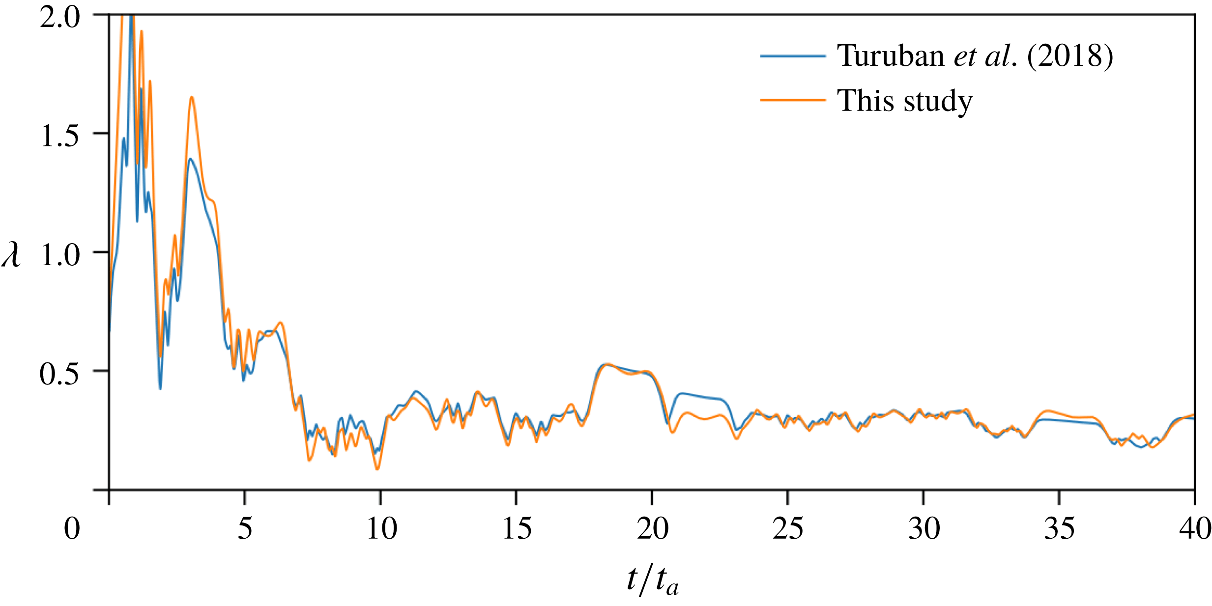
. We subsequently compute the advection equation (2.4) and Lyapunov exponents (detailed in appendix A) for these cases. Soulvaiotis, Jana & Ottino (Reference Soulvaiotis, Jana and Ottino1995) have extensively studied the impact of numerical errors in numerical calculation of both the velocity field and particle advection upon the Lyapunov exponent. Soulvaiotis et al. (Reference Soulvaiotis, Jana and Ottino1995) find that errors in the length of material lines grow with the square of advection time so long as the basic flow is sufficiently resolved. As these errors only grow algebraically in time, these errors do not impact estimation of the Lyapunov exponent.
The underlying symmetries of the velocity field
 $\boldsymbol{v}(\boldsymbol{x})$
play a fundamental role in controlling the Lagrangian kinematics (Franjione et al.
Reference Franjione, Leong and Ottino1989; Mezić & Wiggins Reference Mezić and Wiggins1994; Haller & Mezic Reference Haller and Mezic1998; Yannacopoulos et al.
Reference Yannacopoulos, Mezić, Rowlands and King1998). We denote the symmetry planes on the faces and mid-planes, respectively, of the SC and BCC cubic unit cells as
 $L_{i}^{\pm }$
and
 $L_{i}^{\prime }$
(with
 $i\in \{X,Y,Z\}$
). As shown in figure 2(d), these correspond to the planes oriented normal to the
 $Z$
-coordinate as
 $$\begin{eqnarray}\displaystyle & \displaystyle L_{Z}:Z=\pm \frac{\ell }{2}, & \displaystyle\end{eqnarray}$$
 $$\begin{eqnarray}\displaystyle & \displaystyle L_{Z}^{\prime }:Z=0, & \displaystyle\end{eqnarray}$$
with similar symmetry planes orientated normal to the
 $X$
,
 $Y$
coordinates. The associated reflection symmetries in the
 $Z$
-direction are then
 $$\begin{eqnarray}\displaystyle & \displaystyle {\mathcal{L}}_{Z}:(X,Y,Z)\mapsto (X,Y,-Z\pm \ell ), & \displaystyle\end{eqnarray}$$
 $$\begin{eqnarray}\displaystyle & \displaystyle {\mathcal{L}}_{Z}^{\prime }:(X,Y,Z)\mapsto (X,Y,-Z), & \displaystyle\end{eqnarray}$$
with similar reflections in the
 $X,$
 $Y$
directions. Note that the symmetry planes defined in (2.8), (2.9) constitute a subset of the total reflection symmetries of the SC and BCC lattices described at the start of § 2.1, and all of these symmetry planes repeat throughout the lattice due to periodicity of the unit cell.
The reversibility of Stokes flow means that if the mean flow direction
 $\boldsymbol{q}=(\unicode[STIX]{x1D703}_{f},\unicode[STIX]{x1D719}_{f})$
is oriented normal to any of the reflection symmetries of the granular lattice, then the associated velocity field
 $\boldsymbol{v}(\boldsymbol{x})$
inherits this reflection symmetry, which ultimately constrains the Lagrangian kinematics to be completely regular and integrable. This is shown in figure 1(b), which depicts periodic, integrable streamlines (with zero transverse hydrodynamic dispersion) when the flow direction
 $(\unicode[STIX]{x1D703}_{f},\unicode[STIX]{x1D719}_{f})=(0,0)$
is normal to the
 ${\mathcal{L}}_{X}^{\pm }$
and
 ${\mathcal{L}}_{X}^{\prime }$
reflection symmetries in the BCC lattice. When this symmetry is broken however (e.g. for
 $(\unicode[STIX]{x1D703}_{f},\unicode[STIX]{x1D719}_{f})=(\unicode[STIX]{x03C0}/40,7\unicode[STIX]{x03C0}/90)$
), there is a sharp transition in the Lagrangian kinematics, leading to strong chaotic mixing with significant fluid stretching and folding (and the onset of transverse hydrodynamic dispersion), as shown in figure 1(b). Such breaking of reflection symmetries is also a necessary condition for the onset of chaotic mixing in the SC lattice, although as shown in figure 1(a), significantly weaker mixing results, despite the SC and BCC lattices sharing the same symmetry point group.
These differences in mixing dynamics between the two sphere lattices are further highlighted in figure 3, which shows the distribution of the infinite-time Lyapunov exponent
 $\unicode[STIX]{x1D706}$
over
 ${\mathcal{H}}$
. Here
 $\unicode[STIX]{x1D706}$
is defined in terms of the mean fluid deformation over the entire fluid domain
 ${\mathcal{D}}$
per unit cell length distance
 $\ell$
advected downstream, see appendix A for details. From the distribution of the Lyapunov exponent
 $\unicode[STIX]{x1D706}$
over the parameter space
 ${\mathcal{H}}$
it is then possible to estimate the mean
 $\langle \unicode[STIX]{x1D706}\rangle$
and standard deviation
 $\unicode[STIX]{x1D70E}_{\unicode[STIX]{x1D706}}$
over the ensemble of all flow orientations (see appendix B for details). From figure 3, it is clear that chaotic mixing is significantly stronger and more variable within the BCC lattice (
 $\langle \unicode[STIX]{x1D706}\rangle =0.1280$
,
 $\unicode[STIX]{x1D70E}_{\unicode[STIX]{x1D706}}=0.0856$
) than in the SC lattice (
 $\langle \unicode[STIX]{x1D706}\rangle =0.0240$
,
 $\unicode[STIX]{x1D70E}_{\unicode[STIX]{x1D706}}=0.0133$
). For each flow orientation in
 ${\mathcal{H}}$
, the Lagrangian topology of the flow is illustrated by its corresponding Poincaré section, constructed by recording the intersection of streamlines with the planes shown in figure 2(a,b). A Poincaré section provides an illustration of the Lagrangian kinematics of the flow; it is constructed by recording the intersection of a number of particle trajectories with a 2-D surface (the Poincaré section) embedded within the fluid domain
 ${\mathcal{D}}$
of the unit cell over many flow periods. To construct the Poincaré section, periodic boundary conditions are applied to the particle trajectories within the unit cell such that they intersect multiple times with the Poincaré section. Coherent regions of the Poincaré section correspond to non-mixing regions (i.e. Kolmogorov-Arnol’d-Moser (KAM) islands (Ottino Reference Ottino1989)), whereas regions of apparently random particle locations indicate ergodicity and chaotic dynamics (chaos).
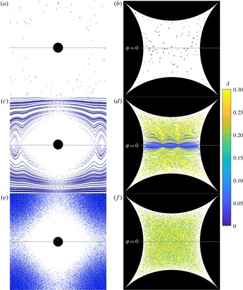
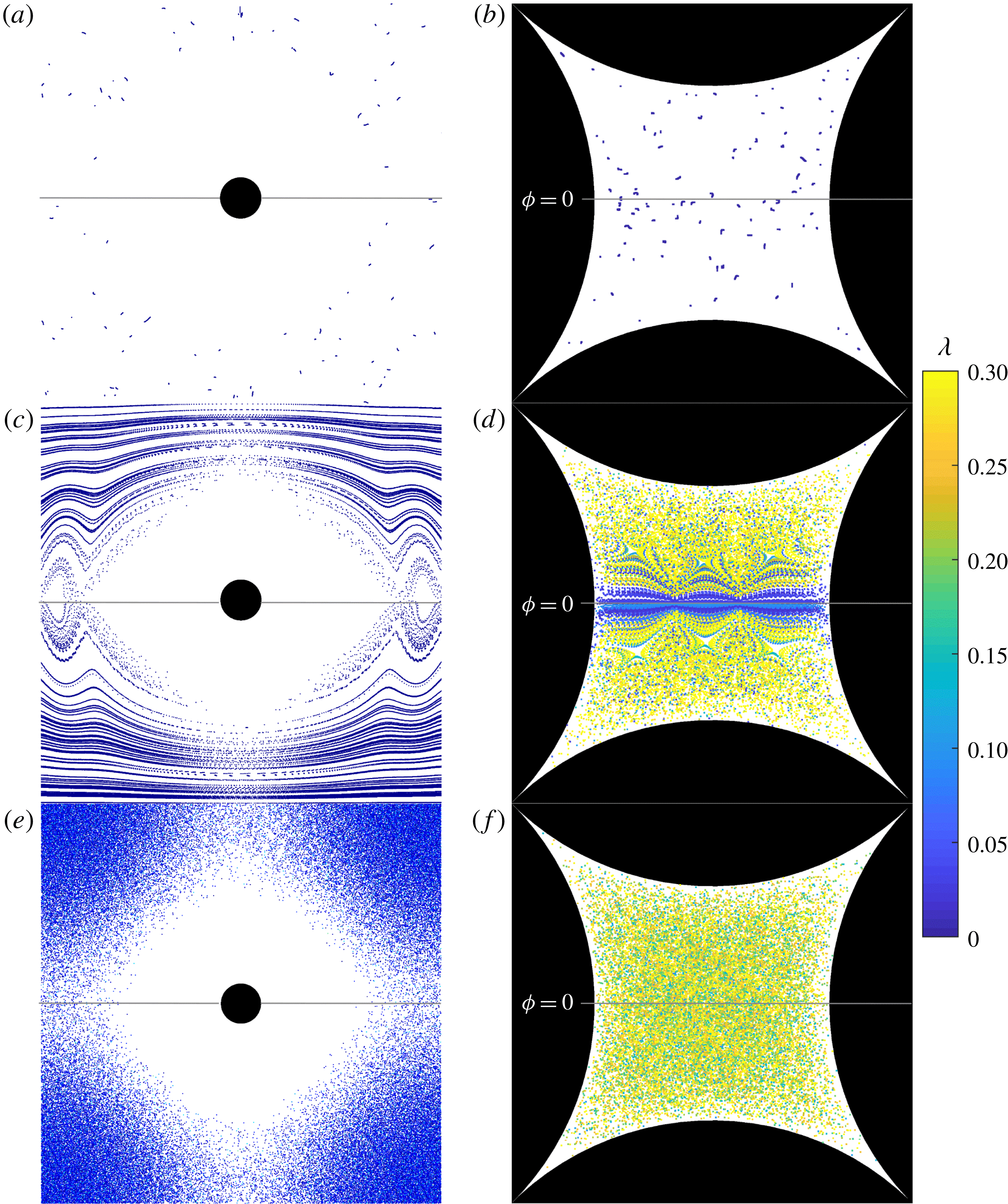
As shown in figure 5(b,d,f), the Poincaré sections evidence a rich array of Lagrangian topologies throughout the BCC flow orientation space, ranging from completely regular (figure 5 b) to mixed regular and chaotic (figure 5 d) to seemingly globally chaotic dynamics (figure 5 f). Conversely, the Lagrangian topologies for the SC lattice are predominantly regular (figure 5 a,c), and the regions which are chaotic (figure 5 e) are only weakly so.
The role of reflection symmetries is highlighted by the completely regular dynamics (with
 $\unicode[STIX]{x1D706}=0$
) observed at the three corners of the parameter space
 ${\mathcal{H}}$
of both the SC and BCC lattices (see, respectively, figures 5(a,c,e) and 5(b,d,f)), which correspond to mean flows oriented normal to their reflection symmetries.
Conversely, there exist very significant differences along the
 $\unicode[STIX]{x1D719}_{f}=0$
transect (where the mean flow is parallel to the
 $L_{Z}$
,
 $L_{Z}^{\prime }$
planes); in the BCC lattice this results in strong chaotic mixing (almost the strongest throughout
 ${\mathcal{H}}$
), whereas for the SC lattice the mixing dynamics is completely regular (
 $\unicode[STIX]{x1D706}=0$
) along
 $\unicode[STIX]{x1D719}_{f}=0$
. These differences in Lagrangian kinematics along
 $\unicode[STIX]{x1D719}_{f}=0$
are then responsible for the much stronger mixing in the BCC lattice throughout the entire parameter space
 ${\mathcal{H}}$
.
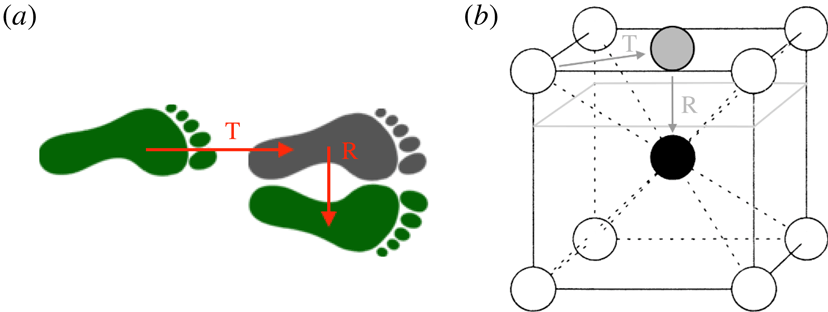
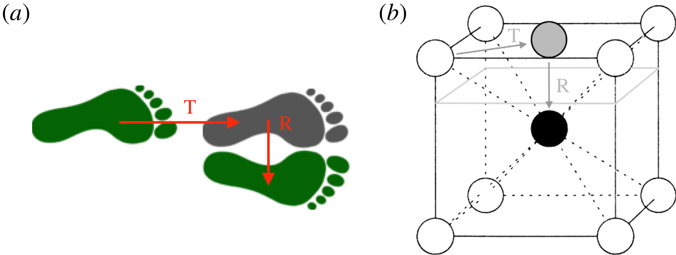
In Turuban et al. (Reference Turuban, Lester, Borgne and Méheust2018), we discovered that the origin of these significant differences in the Lagrangian kinematics are due to the fact that whilst the SC and BCC lattices share the same symmetry point group, their symmetry space groups (which include translations as well as reflections and rotations) differ due to the presence of the central sphere in the BCC unit cell. This additional sphere then admits a set of glide symmetries in the BCC lattice, which are a type of symmetry that consists of a combination of a translation and a reflection. One common example of a glide symmetry is a set of footprints shown in figure 4(a); here the left and right footprints map into each other by translation along the direction of travel and reflection across the travel direction. In the BCC lattice, one glide symmetry arises from translation of an exterior sphere across a unit cell face as shown in figure 4(b), followed by reflection through a plane parallel to this face (denoted by the light grey outline). This combination of translation and reflection is represented by the mapping
 $$\begin{eqnarray}\displaystyle {\mathcal{G}}_{Z}^{\pm }:(X,Y,Z)\mapsto (X+\ell /2,Y+\ell /2,\pm \ell /2-Z), & & \displaystyle\end{eqnarray}$$
and there also exist other similar glide symmetries corresponding to
 $X$
,
 $Y$
reflections. As shown in figure 2(d), these glide symmetries are oriented about the planes
 $G_{Z}^{\pm }:Z=n\ell \pm \ell /4$
, with similar
 $X$
,
 $Y$
glide planes associated with the
 $X$
,
 $Y$
glide symmetries respectively. In the Stokes limit both the sphere lattice and the relative mean flow fully dictate the entire fluid velocity field
 $\boldsymbol{v}(\boldsymbol{x})$
. As such, when the mean flow direction
 $\boldsymbol{q}$
is oriented tangentially to the glide planes
 $G_{Z}^{\pm }$
(i.e. when
 $\unicode[STIX]{x1D719}_{f}=0$
), the local flow field
 $\boldsymbol{v}(\boldsymbol{x})=(v_{X},v_{Y},v_{Z})$
then inherits the glide symmetry (2.10) as
 $$\begin{eqnarray}\displaystyle \left.\begin{array}{@{}c@{}}\displaystyle v_{X}(X,Y,Z)=v_{X}(X+\ell /2,Y+\ell /2,\pm \ell /2-Z),\\ \displaystyle v_{Y}(X,Y,Z)=v_{Y}(X+\ell /2,Y+\ell /2,\pm \ell /2-Z),\\ \displaystyle v_{Z}(X,Y,Z)=-v_{Z}(X+\ell /2,Y+\ell /2,\pm \ell /2-Z).\end{array}\right\} & & \displaystyle\end{eqnarray}$$
The resultant glide symmetry of the velocity field (2.11) itself then generates a series of ‘eggtray’-shaped material surfaces
 ${\mathcal{M}}_{Z}^{\pm }$
in the BCC lattice (material surfaces are defined as being invariant with the flow, and hence consisting of streamlines);
 ${\mathcal{M}}_{Z}^{+}$
and
 ${\mathcal{M}}_{Z}^{-}$
are centred about the planes
 $G_{Z}^{\pm }$
(as shown in figure 2
d) and are invariants of both the flow and the glide symmetries
 ${\mathcal{G}}_{Z}^{\pm }$
.
(a) Glide symmetry associated with a set of footprints, consisting of a translation (T) followed by a reflection (R). (b) Glide symmetry of the BCC unit cell, consisting of a translation (T) of
 $+\ell /2$
in the
 $X$
- and
 $Y$
-direction, followed by a reflection (R) through the plane
 $Z=\ell /4$
, indicated by the light grey outline.
Poincaré sections for the SC (a,c,e) and BCC (b,d,f) lattice for different flow orientations
 $(\unicode[STIX]{x1D703}_{f},\unicode[STIX]{x1D719}_{f})$
. The orientation and location of the planes used to compute the Poincaré section is illustrated in figure 2 for the SC (a) and BCC (b) unit cells. (a,b)
 $(\unicode[STIX]{x1D703}_{f},\unicode[STIX]{x1D719}_{f})=(0,0)$
, (c,d)
 $(\unicode[STIX]{x1D703}_{f},\unicode[STIX]{x1D719}_{f})=(\unicode[STIX]{x03C0}/10,0)$
, (e,f)
 $(\unicode[STIX]{x1D703}_{f},\unicode[STIX]{x1D719}_{f})=(\unicode[STIX]{x03C0}/8,\unicode[STIX]{x03C0}/40)$
. Each particle in the Poincaré sections is shaded according to the finite-time Lyapunov exponent
 $\hat{\unicode[STIX]{x1D706}}$
(A 4) computed along the streamline from its initial location. Note that the same number of initial points were used for all Poincaré sections, but the completely integrable flow in (a) leads to periodic trajectories.
Whilst the shape of the material surface formed by these streamlines can deform with the orientation angle
 $\unicode[STIX]{x1D703}_{f}$
, the gross eggtray shape persists as it is constrained by the glide symmetry
 ${\mathcal{G}}_{Z}^{\pm }$
, where contact points between spheres in the BCC lattice must all belong to the invariant surfaces
 ${\mathcal{M}}_{Z}^{\pm }$
. Turuban et al. (Reference Turuban, Lester, Borgne and Méheust2018) find that the glide symmetries
 ${\mathcal{G}}_{Z}^{\pm }$
and the associated material surfaces are directly responsible for the generation of Lagrangian chaos for mean flows with
 $\unicode[STIX]{x1D719}_{f}=0$
in the BCC lattice. Conversely, the glide symmetries and associated material surfaces do not occur in the SC lattice as there is no central sphere in the unit cell. In § 4 we briefly review the specific mechanisms which generate these chaotic dynamics.
Therefore in these cases it appears that both the reflection and glide symmetries control the mixing dynamics. It is well known that breaking of the reflection symmetry is a necessary condition for the attainment of chaotic dynamics in all flows. The novel observation in Turuban et al. (Reference Turuban, Lester, Borgne and Méheust2018) is that for Stokes flows in the SC and BCC lattices with the mean flow direction oriented along the
 $\unicode[STIX]{x1D719}_{f}=0$
transect, the presence of a glide symmetry is a further necessary condition for chaotic dynamics. The implication of this observation is then that chaotic dynamics is possible for Stokes flows over the BCC and SC lattices which are not constrained to
 $\unicode[STIX]{x1D719}_{f}=0$
, regardless of the presence of a glide symmetry. However, for
 $\unicode[STIX]{x1D719}_{f}\neq 0$
, the strength of chaos in this region of orientation space is influenced by the dynamics along
 $\unicode[STIX]{x1D719}_{f}=0$
, hence weaker mixing overall is observed in the SC lattice than the BCC. The glide symmetry is responsible for this observation.
Thus, in contrast to classical understanding (Szabó & Tél Reference Szabó and Tél1989) that symmetry breaking is connected with the onset of chaotic dynamics, in Turuban et al. (Reference Turuban, Lester, Borgne and Méheust2018) we find that for certain applications glide symmetries can also play a governing role with respect to the generation of Lagrangian chaos. This surprising result may be attributed to the fact that space-group symmetries have received significantly less attention in the study of chaotic dynamical systems than their point-group counterparts. The extent to which this observation applies to other systems which possess space group symmetries is an open question. This observation points to a possible extension of field-invariant symmetry analyses (Mezić & Wiggins Reference Mezić and Wiggins1994; Haller & Poje Reference Haller and Poje1998) based on point-group symmetries to include the impacts of space-group symmetries upon dynamical systems in general and fluid mixing in particular.
It is also interesting to note that the strongest mixing case for the BCC lattice for the points computed in
 ${\mathcal{H}}$
lies on the
 $\unicode[STIX]{x1D719}_{f}=0$
transect. As shall be shown in § 4, along this transect, streamlines (and hence mixing) are confined to material regions that are bound between the
 $L_{Z}$
,
 $L_{Z}^{\prime }$
symmetry planes and the
 ${\mathcal{M}}_{Z}^{\pm }$
material surface (as shown in figure 12
c). This means that for
 $\unicode[STIX]{x1D719}_{f}=0$
there are regions of strong mixing in the flow, however these regions are bound and so the net transverse dispersion is zero. These bounding symmetries (including the glide symmetry
 ${\mathcal{G}}_{Z}^{\pm }$
) are broken by a small perturbation in
 $\unicode[STIX]{x1D719}_{f}$
, resulting in global chaos (defined as chaotic dynamics throughout the entire flow domain) and transverse dispersion. Hence in the BCC lattice the strongest mixing case over
 ${\mathcal{H}}$
arises close to the maximum computed value of
 $\unicode[STIX]{x1D706}$
along
 $\unicode[STIX]{x1D719}_{f}=0$
. In contrast, the SC lattice displays weak mixing throughout the parameter space
 ${\mathcal{H}}$
.
3 Chaotic mixing in discrete porous media
3.1 Mechanisms of chaotic mixing in discrete porous media
In addition to the role of symmetries, it is also instructive to consider the underlying mechanisms for generation of chaotic mixing in discrete (i.e. granular) porous media. Whilst these mechanisms are well established for continuous porous media (i.e. that consisting of a continuous solid phase) (Lester et al.
Reference Lester, Metcalfe and Trefry2013), it is unclear how these mechanisms apply to discrete porous media such as granular matter. In discrete porous media, the point-like nature of the grain contacts renders the fluid–solid boundary non-smooth, invalidating the underlying theorems (e.g. Poincaré–Hopf) central to understanding these mechanisms in continuous media (Lester et al.
Reference Lester, Metcalfe and Trefry2013). As shall be shown, the point-like nature of the contacts between spheres (or grains in the general case) has a significant impact upon the generation of chaotic mixing in discrete porous media. In the following Sections we shall explore the detailed role of these singular grain contacts, and use these insights to develop a predictive model of the Lyapunov exponent distribution over
 ${\mathcal{H}}$
. To begin, we shall first briefly review the mechanisms which lead to chaotic mixing in steady pore-scale flows.
Chaotic advection occurs in steady 3-D flows when 2-D stable
 ${\mathcal{W}}_{2D}^{S}$
and unstable
 ${\mathcal{W}}_{2D}^{U}$
manifolds (shown in figure 7) in the fluid domain
 ${\mathcal{D}}$
intersect transversely (MacKay Reference MacKay2001) to form a homoclinic or heteroclinic tangle, the hallmark of chaos in continuous systems. In steady flows, 2-D stable and unstable manifolds are material surfaces in the flow that are more commonly known in fluid mechanics as flow reattachment and separation surfaces. They respectively undergo exponential contraction and stretching, and are hence termed hyperbolic. Due to volume conservation, these exponentially contracting stable and exponentially expanding unstable manifolds must respectively repel and attract neighbouring fluid streamlines at an exponential rate. Heteroclinic and homoclinic tangles refer to a transverse (non-tangential) intersection of stable and unstable manifolds, where homoclinic refers to manifolds that originate from a common location, and heteroclinic refers to manifolds from different locations. As the steady Stokes flow
 $\boldsymbol{v}(\boldsymbol{x})$
typically does not exhibit flow reversal (aside from e.g. localised Moffatt vortices (Moffatt Reference Moffatt1964)), only heteroclinic intersections (involving un/stable manifolds that originate from different locations) arise as unstable manifolds propagate downstream, whereas stable manifolds propagate upstream. Given the central role of 2-D un/stable manifolds, we shall consider the mechanisms that lead to their generation in discrete porous media and the subsequent formation of transverse heteroclinic intersections, leading to chaotic mixing as illustrated in supplementary movie 2.
As shown by Surana, Grunberg & Haller (Reference Surana, Grunberg and Haller2006), flow separation and reattachment (and hence 2-D un/stable manifolds) are generated by hyperbolic (exponential) stretching of the skin friction field
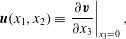 $$\begin{eqnarray}\displaystyle \boldsymbol{u}(x_{1},x_{2})\equiv \left.\frac{\unicode[STIX]{x2202}\boldsymbol{v}}{\unicode[STIX]{x2202}x_{3}}\right|_{x_{3}=0}, & & \displaystyle\end{eqnarray}$$
over the fluid boundary
 $\unicode[STIX]{x2202}{\mathcal{D}}$
(figure 6) on the sphere surfaces, where
 $(x_{1},x_{2})$
and
 $x_{3}$
are tangent and normal respectively to
 $\unicode[STIX]{x2202}{\mathcal{D}}$
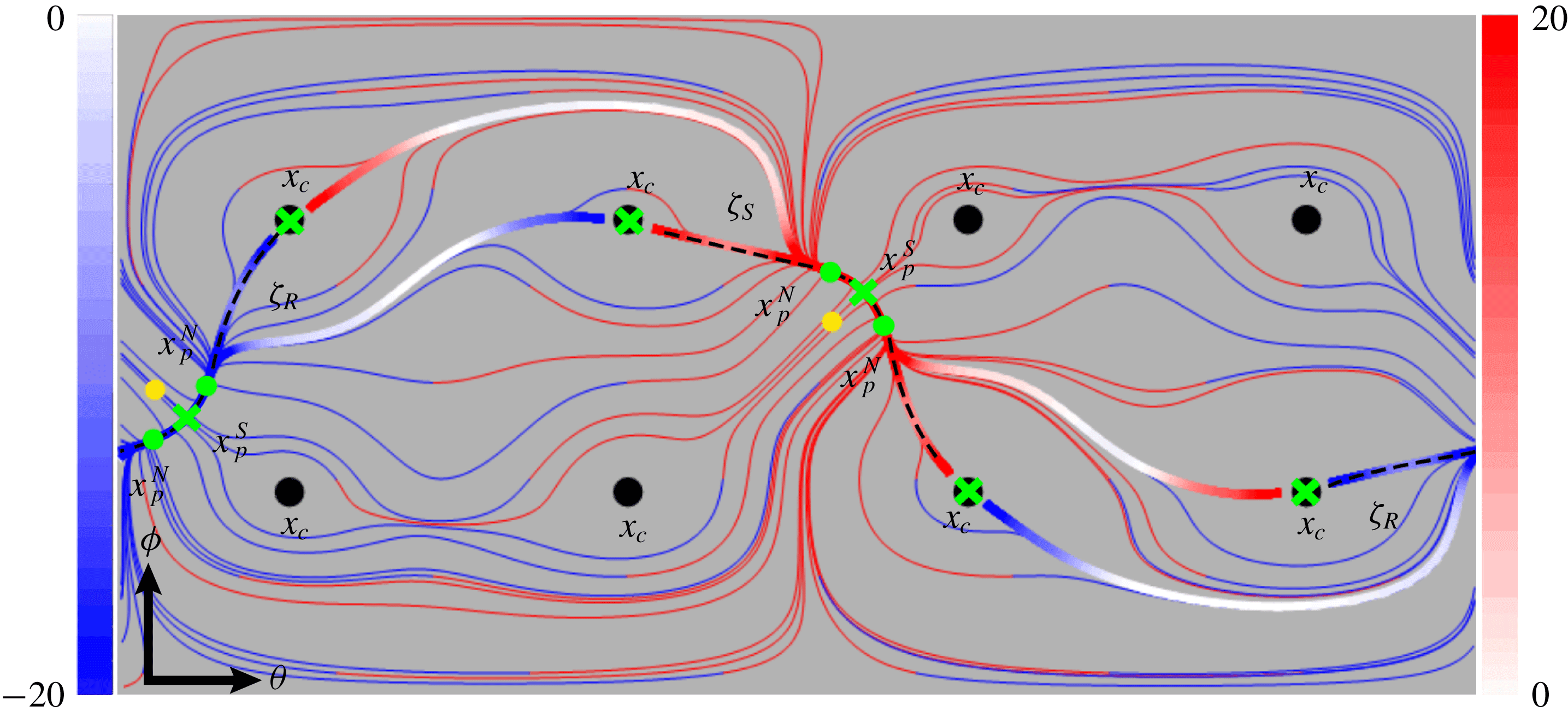
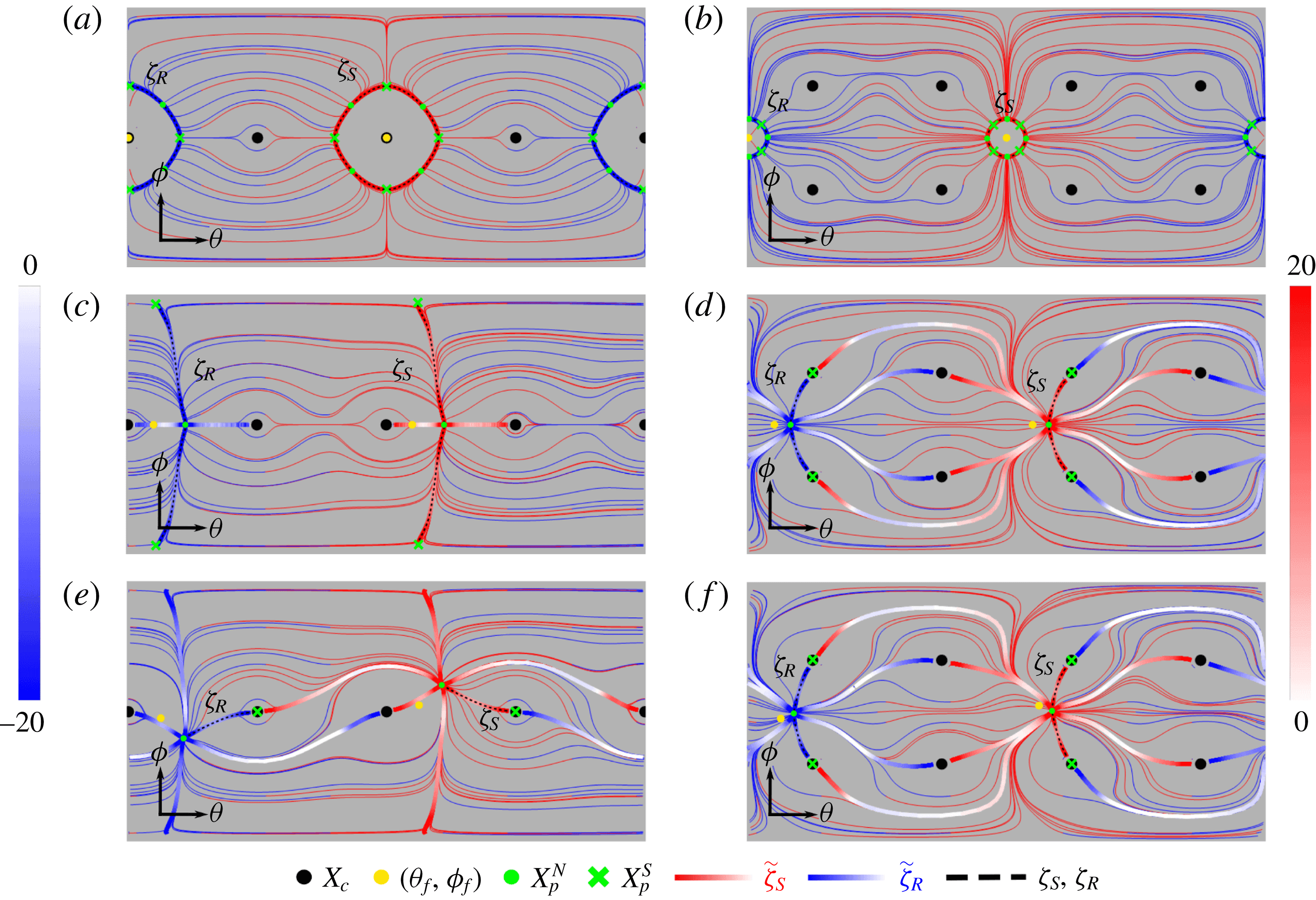
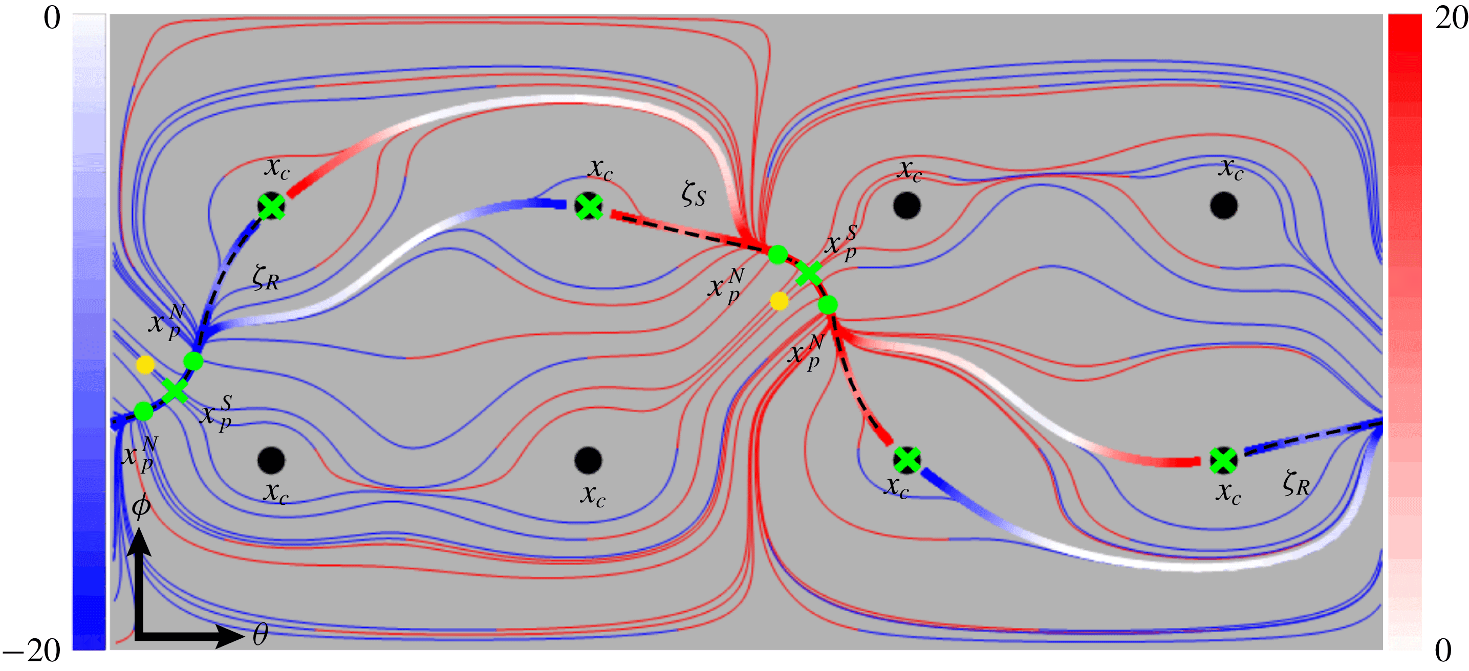
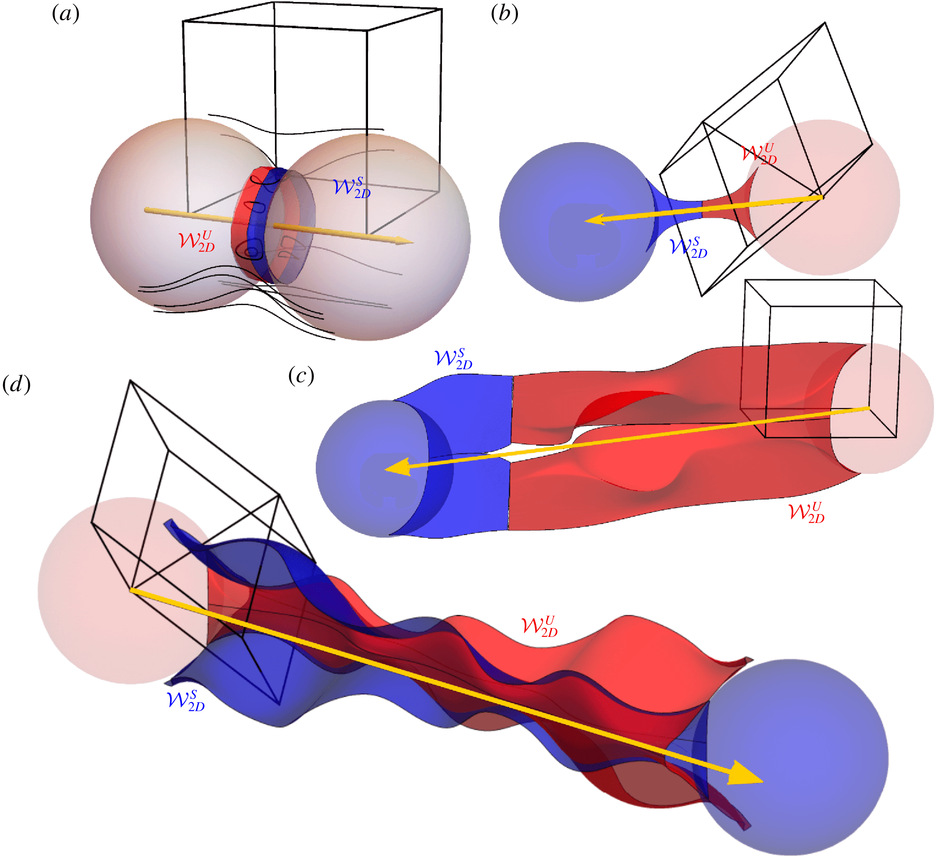
. Typical skin friction fields and associated vector field lines for the SC and BCC lattices are shown in figures 6 and 7(a). Vector field lines that act as strongly hyperbolic (as defined by Surana et al. (Reference Surana, Grunberg and Haller2006)) attractors and repellers in
 $\boldsymbol{u}$
are termed as critical lines
 $\unicode[STIX]{x1D701}$
. From volume conservation, 2-D unstable and stable manifolds are generated respectively by separation
 $\unicode[STIX]{x1D701}_{S}$
(
 $\unicode[STIX]{x1D735}_{\bot }\boldsymbol{\cdot }\boldsymbol{u}<0$
) or reattachment
 $\unicode[STIX]{x1D701}_{R}$
(
 $\unicode[STIX]{x1D735}_{\bot }\boldsymbol{\cdot }\boldsymbol{u}>0$
) critical lines (as shown in figure 7
a), where
 $\unicode[STIX]{x1D735}_{\bot }\equiv (\unicode[STIX]{x2202}_{1},\unicode[STIX]{x2202}_{2},0)$
. Attracting and repelling vector field lines which are not strongly hyperbolic are termed pseudo-critical lines (denoted
 $\hat{\unicode[STIX]{x1D701}}$
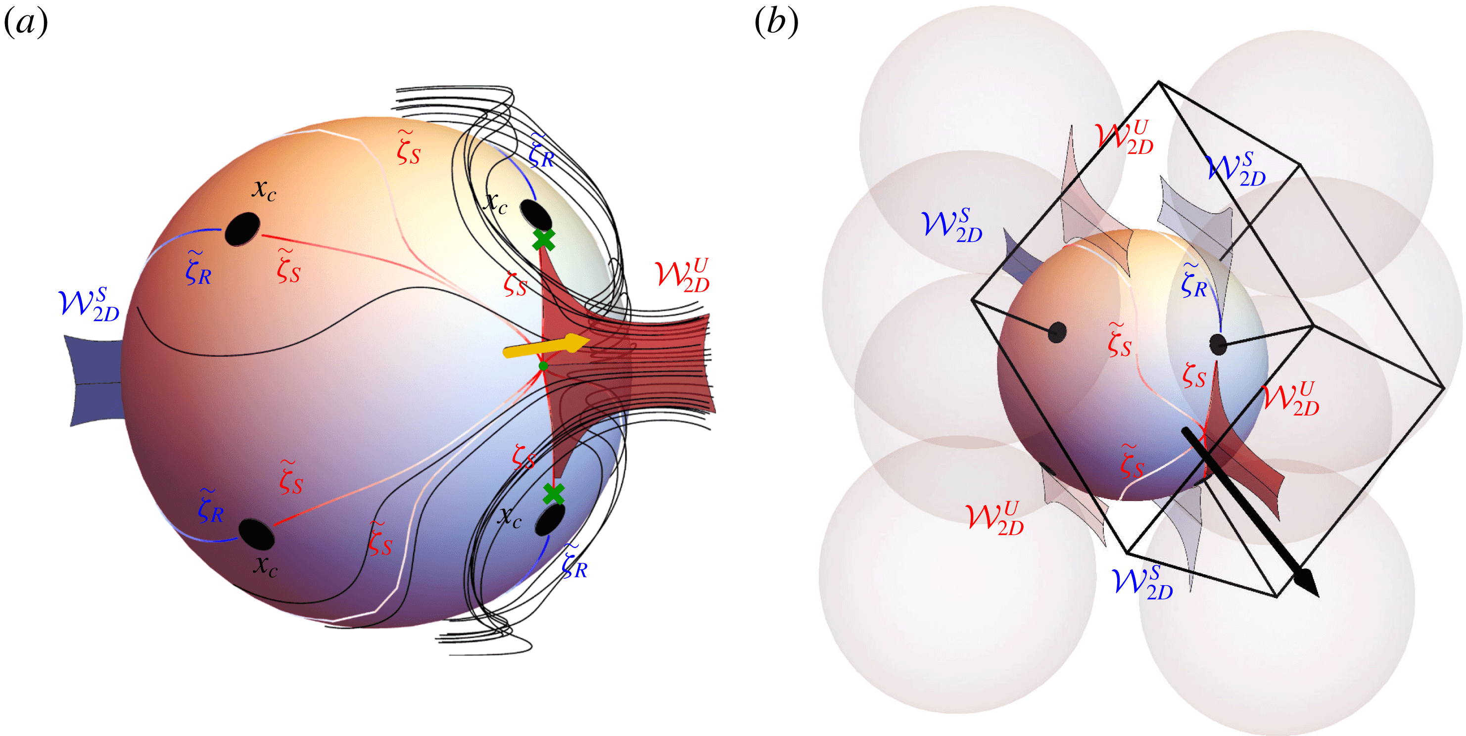
); we find these typically arise from the termination of 2-D un/stable manifolds emanating from neighbouring spheres in the primitive cell (as shown in figure 7
b). We compute the 2-D stable (respectively, unstable) manifolds of the flow by placing tracer particles a small distance
 $\unicode[STIX]{x1D716}\sim 2.5\times 10^{-4}$
(in unit cell sizes) away from the separation (respectively, reattachment) critical lines in the direction normal to the sphere surface, and advect these particles backwards (respectively, forwards) in time. Due to exponential contraction (respectively, expansion) of the stable (respectively, unstable) manifold itself, particles are attracted to these manifolds in backwards (respectively, forwards) time, so any small error in the initial position of the tracer with respect to the true manifold location decays exponentially.
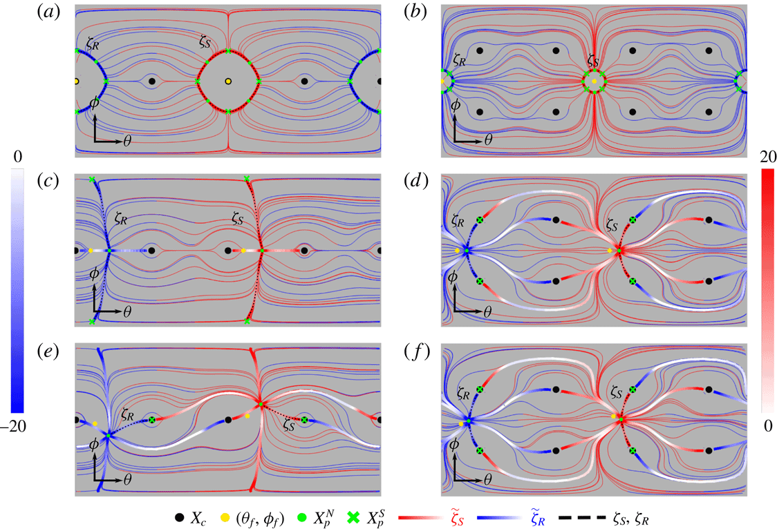
Forward (light grey (red online)) and backward (dark grey (blue online)) field lines (thin) of the skin friction field
 $\boldsymbol{u}$
over the sphere surface
 ${\mathcal{D}}$
(in terms of the spherical coordinates
 $(\unicode[STIX]{x1D703},\unicode[STIX]{x1D719})$
) corresponding to the cases (a–f) described in figure 5. Due to periodicity all spheres share the same skin friction field. Also shown are the mean flow orientation (light grey, (yellow online) dots), node
 $\boldsymbol{x}_{p}^{N}$
(light grey (green online) dots), saddle
 $\boldsymbol{x}_{p}^{S}$
(light grey (green online) crosses) and contact
 $\boldsymbol{x}_{c}$
points (black discs). The separation (light grey (red online)) and reattachment (dark grey (blue online)) critical
 $\unicode[STIX]{x1D701}$
(thick, black dashed) and pseudo-critical
 $\tilde{\unicode[STIX]{x1D701}}$
lines (thick) are coloured according to
 $(\unicode[STIX]{x1D735}_{\bot }\boldsymbol{\cdot }\boldsymbol{u})/\Vert \boldsymbol{u}\Vert$
.
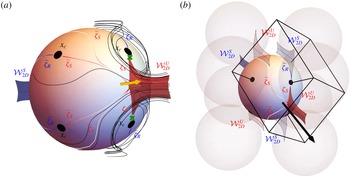
(a) Three-dimensional view of the skin friction field shown in figure 6(f), showing fluid streamlines (black), stable
 ${\mathcal{W}}_{2D}^{S}$
(dark grey (blue online)) and unstable
 ${\mathcal{W}}_{2D}^{U}$
(light grey (red online)) 2-D manifolds emanating from pseudo-critical
 $\tilde{\unicode[STIX]{x1D701}}$
and critical lines
 $\unicode[STIX]{x1D701}$
. (b) Same as for (a) but with primitive cell (black lines) and neighbouring spheres and associated (transparent) periodic translations of the separation (
 ${\mathcal{W}}_{2D}^{U}$
) and reattachment (
 ${\mathcal{W}}_{2D}^{S}$
) surfaces, indicating the pseudo-critical lines
 $\tilde{\unicode[STIX]{x1D701}}$
arise as non-hyperbolic intersections of these translated manifolds with the reference spheres. See supplementary movies 3 and 4 for 3-D animations of this figure. Adapted from Turuban et al. (Reference Turuban, Lester, Borgne and Méheust2018).
All critical lines in the skin friction field
 $\boldsymbol{u}$
must terminate at either stable spirals, limit cycles or critical points
 $\boldsymbol{x}_{p}$
. Whilst stable spirals and limit cycles can occur in discrete porous media due to the presence of Moffatt vortices (Moffatt Reference Moffatt1964) near contact points, in practice Moffatt vortices are rare. Across all simulations we only observe Moffatt vortices for the flow orientation
 $(\unicode[STIX]{x1D703}_{f},\unicode[STIX]{x1D719}_{f})=(0,0)$
(reflecting observations (Davis et al.
Reference Davis, O’Neill, Dorrepaal and Ranger1976) of such vortices for two isolated spheres aligned with the mean flow direction), but none are apparent for any other flow orientation.
Hence we focus our attention upon the formation of critical lines from critical points. Critical points, defined as
 $\boldsymbol{u}(\boldsymbol{x}_{p})=\mathbf{0}$
, are characterised in terms of the linearised skin friction tensor
 $$\begin{eqnarray}\displaystyle \left.\unicode[STIX]{x1D63C}\equiv \frac{\unicode[STIX]{x2202}\boldsymbol{u}}{\unicode[STIX]{x2202}\boldsymbol{x}}\right|_{\boldsymbol{x}=\boldsymbol{x}_{p}}, & & \displaystyle\end{eqnarray}$$
which is the boundary counterpart of the strain-rate tensor
 $\unicode[STIX]{x1D641}=\unicode[STIX]{x2202}\boldsymbol{v}/\unicode[STIX]{x2202}\boldsymbol{x}|_{\boldsymbol{x}=\boldsymbol{x}_{0}}$
that quantifies fluid deformation local to interior stagnation points
 $\boldsymbol{x}_{0}$
. Critical points are termed non-degenerate if
 $\det (\unicode[STIX]{x1D63C})\neq 0$
, i.e. fluid deformation local to
 $\boldsymbol{x}_{p}$
can be quantified to leading order in terms of
 $\unicode[STIX]{x1D63C}$
. For incompressible flow the eigenvalues
 $\unicode[STIX]{x1D708}_{i}$
of
 $\unicode[STIX]{x1D641}$
satisfy
 $\sum _{i=1}^{3}\unicode[STIX]{x1D708}_{i}=\unicode[STIX]{x1D735}\boldsymbol{\cdot }\boldsymbol{v}=0$
, whereas the eigenvalues
 $\unicode[STIX]{x1D702}_{i}$
of
 $\unicode[STIX]{x1D63C}$
satisfy
 $\sum _{i=1}^{3}\unicode[STIX]{x1D702}_{i}=\unicode[STIX]{x1D735}\boldsymbol{\cdot }\boldsymbol{u}=-\unicode[STIX]{x1D702}_{3}$
, where
 $\unicode[STIX]{x1D702}_{1}$
and
 $\unicode[STIX]{x1D702}_{2}$
have corresponding eigenvectors tangent to the skin friction boundary
 $\unicode[STIX]{x2202}{\mathcal{D}}$
, while
 $\unicode[STIX]{x1D702}_{3}$
has a corresponding eigenvector normal to
 $\unicode[STIX]{x2202}{\mathcal{D}}$
.
Hence the attraction/repulsion of vector lines to critical points and lines in the skin friction field are directly related to flow separation/reattachment, where
 $\unicode[STIX]{x1D702}_{3}$
characterises the rate of stretching (and thus separation/attachment) rate of the associated 2-D un/stable manifolds. Non-degenerate critical points
 $\boldsymbol{x}_{p}$
may then be classified respectively as node
 $\boldsymbol{x}_{p}^{N}$
, saddle
 $\boldsymbol{x}_{p}^{S}$
or centre
 $\boldsymbol{x}_{p}^{C}$
points based on whether the real parts of
 $\unicode[STIX]{x1D702}_{1}$
,
 $\unicode[STIX]{x1D702}_{2}$
have the same sign, different sign or are both zero. Figure 6 illustrates the diversity of skin friction field topologies observed in the SC and BCC lattices; here the impact of lattice symmetries can be observed, along with the formation of non-degenerate critical points, critical and pseudo-critical lines. In general, the critical points and their type (saddle, node, centre) play a key role in organising the topology of the skin friction field and hence flow separation and reattachment. An exception arises for degenerate critical points, in which case higher order (i.e. higher than first order in (3.2)) expansion of the skin friction field
 $\boldsymbol{u}$
is required to characterise local deformation.
Surana et al. (Reference Surana, Grunberg and Haller2006) use the Poincaré–Bendixson theorem and invariant manifold theory to show that only four types of critical lines are structurally stable (i.e. have stable topology with respect to second-order perturbations of the flow), and only one of these does not involve spirals or limit cycles. The remaining critical line type is formed by the connection between a saddle point and node point, as shown in figure 6. As such, the presence of non-degenerate saddle points in
 $\boldsymbol{u}$
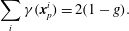
are necessary for the formation of 2-D un/stable manifolds in the fluid interior. For any differentiable (smooth) manifold, the number of saddle points is related to the Poincaré–Hopf theorem, which connects the indices
 $\unicode[STIX]{x1D6FE}$
of the critical points
 $\boldsymbol{x}_{p}$
(where
 $\unicode[STIX]{x1D6FE}=-1,0,1,$
for saddles, centres and nodes respectively) to the topological genus
 $g$
(which quantifies the number of handles or holes an object has; i.e. a sphere has genus zero, a torus genus one, a pretzel genus two or more) of the manifold according to
 $$\begin{eqnarray}\displaystyle \mathop{\sum }_{i}\unicode[STIX]{x1D6FE}(\boldsymbol{x}_{p}^{i})=2(1-g). & & \displaystyle\end{eqnarray}$$
This theorem was used by Lester et al. (Reference Lester, Metcalfe and Trefry2013) to form a lower bound for the number density of saddle points in continuous porous media (such as open porous networks) based upon topological complexity of the porous medium, as characterised by the number density of the topological genus
 $g$
, which is typically large for such porous materials. In turn, this lower bound suggests a significant number density of 2-D un/stable manifolds emanate from the skin friction field at the fluid–solid boundary
 $\unicode[STIX]{x2202}{\mathcal{D}}$
, which can lead to chaotic mixing in continuous porous media. In principle, this mechanism also applies to discrete porous media, as the large number density of particle contacts means the number density of the topological genus must also be large. However the cusp-shaped contacts between particles renders the fluid–solid boundary
 $\unicode[STIX]{x2202}{\mathcal{D}}$
non-smooth, and so the Poincaré–Hopf theorem does not apply to such non-differentiable manifolds, as shown in figure 8. In the following we explore the implications of this result upon chaotic mixing in discrete porous media.
3.2 Topology of discrete porous media and implications for mixing
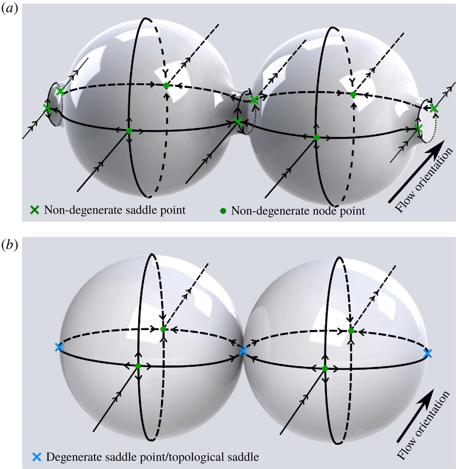
(a) The simplest possible skin friction skeleton for a periodic array of laterally connected spheres with smooth contacts. Negative curvature of the solid surface local to the contact region promotes the formation of saddle points, whilst node points form on the positively curved sphere surfaces. (b) Simplest possible skin friction skeleton for the same system with cusp-shaped contacts. Here the pairs of non-degenerate saddle points shown in (a) coalesce into a single topological saddle point which is degenerate.
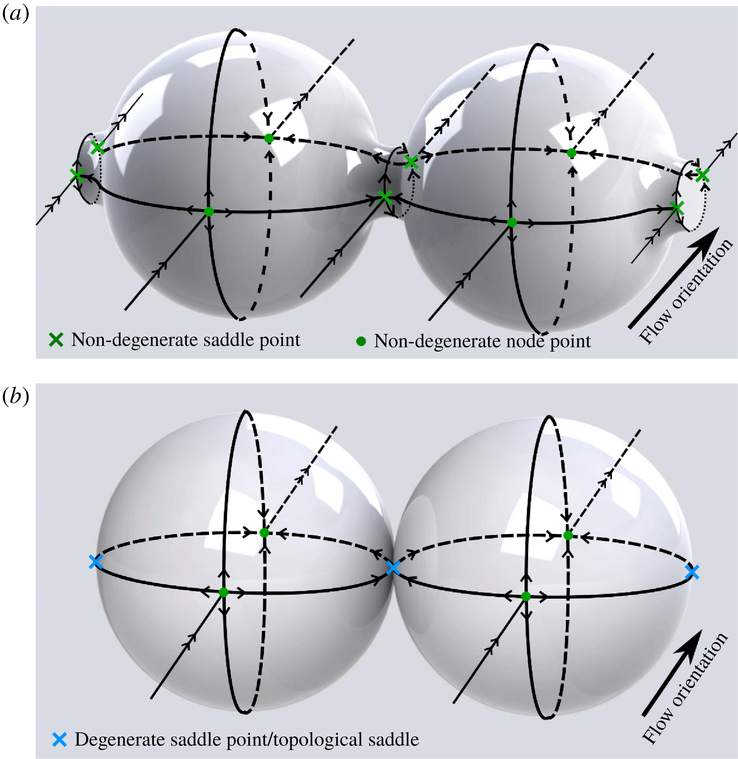
Whilst The Poincaré–Hopf theorem (3.3) does not apply to non-smooth manifolds, it is useful to consider a similar smooth manifold such as that depicted in figure 8(a), where the cusp-shaped sphere contacts have been smoothed to form finite-sized contacts. Figure 8(a) shows the simplest possible skin friction skeleton (comprising of critical points and critical lines) for a periodic array of laterally connected spheres, whereas figure 8(b) shows the corresponding system for cusp-shaped, non-smooth contacts. As saddle points tend to form on surface regions of negative curvature, whereas nodes tend to form on surface regions of positive curvature, the nodes in figure 8(a) arise on the sphere surfaces, whereas the saddle points are localised to the contact regions. For each sphere in the lateral array (which has a total topological genus of one when accounting for periodicity), the Poincaré–Hopf theorem predicts an equal number of nodes and saddles (accounting for the sharing of saddle points at contacts), resulting in the distribution shown in figure 8(a). If we then consider shrinking the smooth, finite contacts in figure 8(a) to form the point-wise, non-smooth contacts in figure 8(b), the negative curvature of these contacts diverges to form a cusp, and the pair of non-degenerate saddle points coalesce into a single degenerate topological saddle. As these saddle points are degenerate, the simplest possible skin friction skeleton (figure 8 b) is the same as that for an isolated sphere.
The role of grain contacts is also illustrated by the Gauss–Bonnett theorem, which connects the mean Gaussian curvature
 $\langle {\mathcal{C}}_{G}\rangle =(1/V)\int _{S\in \unicode[STIX]{x2202}{\mathcal{D}}}{\mathcal{C}}_{1}{\mathcal{C}}_{2}\,\text{d}S$
(with
 ${\mathcal{C}}_{1}$
,
 ${\mathcal{C}}_{2}$
the local principle curvatures,
 $V$
the sphere volume) to the topological genus
 $g$
as
 $$\begin{eqnarray}\displaystyle \langle {\mathcal{C}}_{G}\rangle =4\unicode[STIX]{x03C0}(1-g/V). & & \displaystyle\end{eqnarray}$$
A continuous porous medium is characterised by a large topological genus
 $g$
per unit volume, hence
 $\langle {\mathcal{C}}_{G}\rangle$
is strongly negative and the pore geometry is predominantly hyperbolic, promoting formation of non-degenerate saddle points (Lester et al.
Reference Lester, Metcalfe and Trefry2013). For discrete media
 $g$
is also large and the mean curvature
 $\langle {\mathcal{C}}_{G}\rangle$
is also strongly negative, but now the negative curvature (and hence saddle points) is localised to the cusp-shaped contact points
 $\boldsymbol{x}_{c}$
(whilst the spheroidal grains have predominantly positive curvature), rendering these saddle points degenerate.
For a lattice of spheres with finite-sized connections the topological genus per sphere is
 $g=n_{c}/2$
, where
 $n_{c}$
is the number of contacts
 $\boldsymbol{x}_{c}$
per sphere, as each pair of periodic contact points on the spheres forms a topological ‘handle’ once periodicity of the lattice is taken into account. Hence
 $g=3$
,
 $4$
for the SC and BCC lattices respectively (note that only 4 contact points are apparent for the SC lattices shown in figure 6 as the contact points at
 $\unicode[STIX]{x1D719}=\pm \unicode[STIX]{x03C0}/2$
are not shown). If we denote
 $n_{n}$
as the number of node points per sphere, then from (3.3), the number
 $n_{s}$
of non-degenerate saddle points per sphere is
 $$\begin{eqnarray}\displaystyle n_{s}=n_{n}+n_{c}-2, & & \displaystyle\end{eqnarray}$$
i.e. from figure 8(a), there are two node points per spheres, two contact points and two non-degenerate saddle points (due to periodicity).
In the limit of vanishing contact area, these non-degenerate saddle points coalesce into a topological saddle (Brøns & Hartnack Reference Brøns and Hartnack1999), as shown in figure 8(b). This degenerate saddle point has index
 $\unicode[STIX]{x1D6FE}=-2$
(Brøns & Hartnack Reference Brøns and Hartnack1999), and so we may augment (3.5) to include the number
 $n_{d}$
of degenerate topological saddles for point-wise contacts as
 $$\begin{eqnarray}\displaystyle n_{s}+2n_{d}=n_{n}+n_{c}-2. & & \displaystyle\end{eqnarray}$$
As such, the Poincaré–Hopf theorem can be extended to non-smooth manifolds via suitable treatment of local critical points in the neighbourhood of the contact points. If each pair of contact points
 $\boldsymbol{x}_{c}$
yields a degenerate saddle (
 $n_{c}=2n_{d}$
), then the number of non-degenerate saddles is then related to the number of nodes as
 $$\begin{eqnarray}\displaystyle n_{s}=n_{n}-2. & & \displaystyle\end{eqnarray}$$
Compared to (3.5), (3.7) is the same relationship as for an isolated spheroid, i.e.
 $n_{c}=g=0$
. Therefore, for discrete porous media the simplest possible skin friction field over each particle involves two non-degenerate node points on the sphere surfaces and
 $n_{c}$
degenerate topological saddle points at the grain contact points
 $\boldsymbol{x}_{c}$
, as shown in figure 8(b). The simplest possible non-degenerate skin friction field then has the same topology as that of an isolated sphere with genus
 $g=0$
, i.e. two non-degenerate node points (as reflected by (3.7)).
As such, the basic topological complexity of discrete (granular) porous media alone is not sufficient to generate 2-D un/stable manifolds in the fluid interior due to the degenerate nature of the topological saddle points. This is in contrast to continuous porous media, which must admit a large number density of non-degenerate saddle points and hence 2-D un/stable manifolds (Lester et al. Reference Lester, Metcalfe and Trefry2013). This may appear surprising as the basic mechanism for mixing is the same in both systems: impingement of fluid streams on solid surfaces, implying flow separation and exponential stretching. Both discrete and continuous porous media contain regions of the solid surface which have negative curvature and so saddle points tend to arise in these regions. Discrete porous media also have regions of positive curvature (i.e. the spheres or grains themselves) at which node points tend to accumulate, whereas continuous porous media have a predominantly negative curvature throughout (although there may be local exceptions) and so node points are less likely.
The major difference between these systems however is that discrete porous media involve regions of divergent negative curvature (cusps) which render the saddle points degenerate, as discussed above. These point-wise contacts also render the effective topological genus of each grain as zero; a contact point is neither a node nor a saddle of the skin friction field, but is rather a degenerate point, akin to a centre (with index zero). As such, the physical interactions of the flow are quite different in the two systems; continuous porous media have predominantly non-degenerate saddle points throughout with few nodes, whereas discrete porous media have an even mix of non-degenerate nodes and degenerate saddles. As non-degenerate saddles generate chaos, chaotic advection is inherent to continuous porous media but not to discrete porous media. By inherent, we mean that chaotic mixing in continuous media does not require a bifurcation away from the simplest possible skin friction field, whereas chaotic mixing in discrete media does.
Despite this restriction, discrete porous media can still exhibit 2-D flow separation and chaotic mixing if the skin fiction field bifurcates away from the simplest possible topological state (as determined by (3.6)). The flow topology can lead to (i) bifurcation of the degenerate topological saddles to non-degenerate saddle points (e.g. figure 6 e,d,f) or (ii) bifurcation of node points in the skin friction field into an isolated saddle point and a pair of nodes (e.g. figure 9). As the skin friction field topology on the grains is controlled by the mean flow orientation with respect to the lattice, the presence or absence of chaotic advection depends upon this orientation, in contrast to continuous porous media for which chaotic advection is expected for all but perfectly symmetric media (Lester et al. Reference Lester, Metcalfe and Trefry2013).
Skin friction field over a sphere in the BCC lattice for flow orientation
 $(\unicode[STIX]{x1D703}_{f},\unicode[STIX]{x1D719}_{f})=(\unicode[STIX]{x03C0}/20,\unicode[STIX]{x03C0}/20)$
, illustrating the bifurcation of simplest possible skin friction topology (as discussed in § 3.2) to admit a pair of node points
 $\boldsymbol{x}_{p}^{N}$
and an isolated non-degenerate saddle point
 $\boldsymbol{x}_{p}^{S}$
. This in contrast to the skin friction fields shown in figure 6(c–f) which only contain saddle points which are degenerate.
More generally, the non-inherent nature of the non-degenerate saddle points (and hence 2-D flow separation) in discrete porous media means fluid mixing in such media differs markedly from that of continuous media. This fundamental difference may explain the weaker mixing observed for the sphere lattices herein (with mean Lyapunov exponent
 $\langle \unicode[STIX]{x1D706}\rangle \approx 0.0760$
averaged over both the SC and BCC lattices), compared to the open porous networks considered in Lester et al. (Reference Lester, Metcalfe and Trefry2013) (where
 $\langle \unicode[STIX]{x1D706}\rangle \approx 0.1178$
). Note that discrete porous media considered herein are ordered and the mean Lyapunov exponents for the SC and BCC lattices (
 $\langle \unicode[STIX]{x1D706}\rangle \approx 0.0240$
,
 $\langle \unicode[STIX]{x1D706}\rangle \approx 0.1280$
respectively) span the measured value (
 $\langle \unicode[STIX]{x1D706}\rangle \approx 0.1178$
) for the continuous porous media studied in Lester et al. (Reference Lester, Metcalfe and Trefry2013). Whilst this value was reported for a random open porous network, it was shown (Lester et al.
Reference Lester, Metcalfe and Trefry2013) that this value also corresponds to the ensemble average of the Lyapunov exponent over the ensemble of all possible ordered configurations of the open porous network. Whether this behaviour extends to discrete porous media is an open question, and further work on chaotic mixing in random discrete systems is required to answer this question and to firmly establish whether random discrete or continuous porous media exhibits stronger chaotic mixing.
4 Intersections of stable and unstable 2-D manifolds
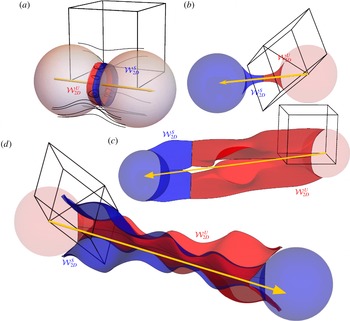
Given formation of stable and unstable 2-D manifolds in the fluid interior, chaotic mixing occurs when these manifolds intersect transversely and so form a heteroclinic tangle, as shown in figure 10(d). Conversely, the Lagrangian kinematics are completely regular if smooth connections arise between un/stable 2-D manifolds, as shown in figure 10(a–c). These 2-D unstable (stable) manifolds are computed by advecting fluid particles which are positioned close to the separation (reattachment) critical lines of the skin friction field forward (backward) in time.
(a–c) Smooth heteroclinic connections for (a) the SC lattice with
 $(\unicode[STIX]{x1D703}_{f},\unicode[STIX]{x1D719}_{f})=(0,0)$
, (b) the BCC lattice with
 $(\unicode[STIX]{x1D703}_{f},\unicode[STIX]{x1D719}_{f})=(\unicode[STIX]{x03C0}/4,0)$
and (c) the SC lattice with
 $(\unicode[STIX]{x1D703}_{f},\unicode[STIX]{x1D719}_{f})=(3\unicode[STIX]{x03C0}/20,0)$
(see also corresponding 3-D animation supplementary movie 5). (d) Transverse heteroclinic intersection for the BCC lattice with
 $(\unicode[STIX]{x1D703}_{f},\unicode[STIX]{x1D719}_{f})=(\unicode[STIX]{x03C0}/20,0)$
(also see corresponding 3-D animation supplementary movie 2). Adapted from Turuban et al. (Reference Turuban, Lester, Borgne and Méheust2018).
As expected, we only observe smooth heteroclinic connections between stable and unstable manifolds for all mean flows which are oriented normal to the reflection symmetry planes of the SC and BCC lattices, as shown in figure 10(a,b). In the specific case where the mean flow is oriented along the crystal axis
 $(\unicode[STIX]{x1D703}_{f},\unicode[STIX]{x1D719}_{f})=(0,0)$
of the SC lattice, a rare example of a recirculation (Moffatt) vortex arises between the spheres (Davis et al.
Reference Davis, O’Neill, Dorrepaal and Ranger1976), and the corresponding un/stable manifolds form a smooth connection, as shown in figure 10(a). For mean flows which are not oriented normal to a symmetry plane, transverse heteroclinic intersections (figure 10
d) mostly arise, however smooth connections can also occur (figure 10
c).
For all flows computed in both lattices we only observe smooth heteroclinic connections between un/stable manifolds that emanate from neighbouring spheres (i.e. those common to a single primitive cell), as shown in figure 10(a,b). We attribute this observation to the fact that there is no object (and hence mechanism) between these spheres to perturb the manifold interactions away from a smooth connection. We also note that for all cases computed, intersection of 2-D un/stable manifolds with other spheres in the primitive cell are responsible for the formation of pseudo-critical lines in the skin friction field, as shown in figure 7(b). As such, critical lines
 $\unicode[STIX]{x1D701}$
in the skin friction field
 $\boldsymbol{u}$
are responsible for the generation of 2-D un/stable manifolds, while pseudo-critical lines
 $\hat{\unicode[STIX]{x1D701}}$
arise from the subsequent collision of these manifolds with spheres upstream or downstream for stable and unstable manifolds respectively.
To understand the impact of the sphere lattice structure upon mixing dynamics and develop a predictive model for the Lyapunov exponent distribution over
 ${\mathcal{H}}$
, we focus attention upon the set of flow orientations
 $\unicode[STIX]{x1D719}_{f}=0$
in
 ${\mathcal{H}}$
, where the differences in Lagrangian kinematics between the SC (regular) and BCC (globally chaotic) lattices are most pronounced. Turuban et al. (Reference Turuban, Lester, Borgne and Méheust2018) showed that these differences can be explained by the presence of the space-group glide symmetry (2.10) in the BCC lattice, which we briefly summarise as follows.
For
 $\unicode[STIX]{x1D719}_{f}=0$
the mean flow is oriented parallel to the reflection symmetry planes
 $L_{Z}$
,
 $L_{Z}^{\prime }$
(figure 2
d), and
 $L_{Z}$
acts a material surface. The intersections of
 ${\mathcal{W}}_{2D}^{S}$
,
 ${\mathcal{W}}_{2D}^{U}$
with
 $L_{Z}$
are streamlines which we respectably denote as
 $\unicode[STIX]{x1D6FC}^{S}$
,
 $\unicode[STIX]{x1D6FC}^{U}$
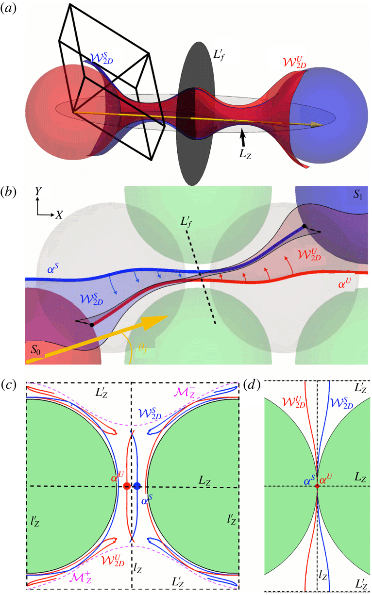
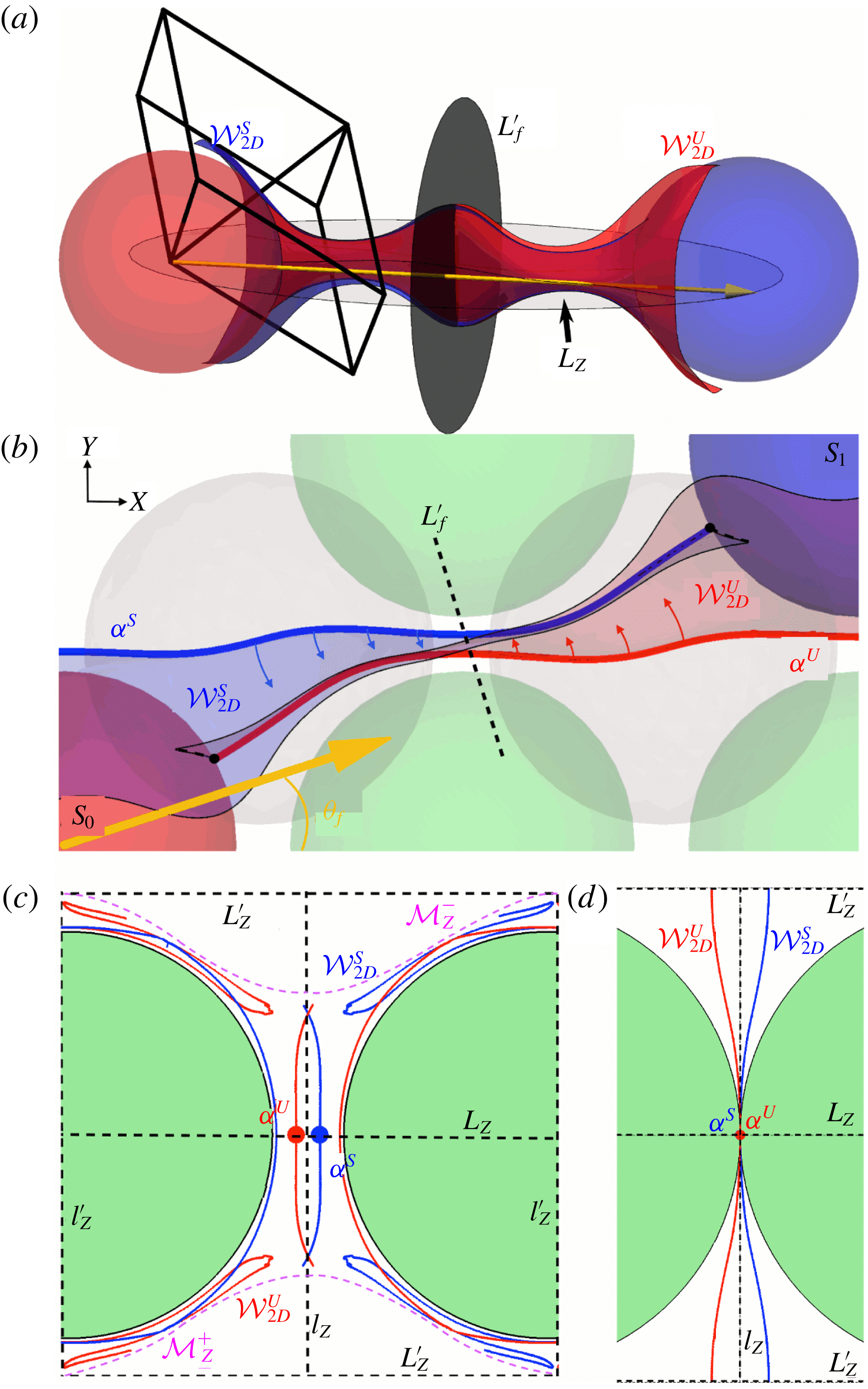
respectively. As they are material lines, these streamlines can only form smooth connections if they intersect (figure 11
b), however transverse intersections of the associated 2-D un/stable manifolds are possible away from the
 $L_{Z}$
plane, as shown in figure 11(c).
We denote the symmetry plane normal to the mean flow direction as
 $L_{f}^{\prime }$
(shown in figure 11
a,b). The intersection of
 ${\mathcal{W}}_{2D}^{S}$
,
 ${\mathcal{W}}_{2D}^{U}$
with
 $L_{f}^{\prime }$
is doubly symmetric in both the BCC (figure 11
c) and SC (figure 11
d) lattices. These two symmetries manifests as a reflection symmetry about
 $L_{Z}$
,
 $L_{Z}^{\prime }$
, and as a reflection-reversal symmetry about the lines
 $l_{Z}$
,
 $l_{Z}^{\prime }$
shown in (figure 11
c,d), which involves exchange between the stable and unstable manifolds. This reflection-reversal symmetry is due to the combination of the
 $L_{Y}$
,
 $L_{X}$
reflection symmetries and the time-reversal symmetry between
 ${\mathcal{W}}_{2D}^{S}$
,
 ${\mathcal{W}}_{2D}^{U}$
. As such, the un/stable 2-D manifolds
 ${\mathcal{W}}_{2D}^{S}$
,
 ${\mathcal{W}}_{2D}^{U}$
can only connect smoothly across
 $L_{Z}$
,
 $L_{Z}^{\prime }$
, whereas transverse intersections are possible across
 $l_{Z}$
,
 $l_{Z}^{\prime }$
, as shown in figure 11(c,d).
For the SC lattice there is no mechanism to generate the energetically unfavourable (due to the minimum dissipation theorem for Stokes flow (Kim & Karrila Reference Kim and Karrila1991)) transverse intersections across
 $l_{Z}$
,
 $l_{Z}^{\prime }$
, hence the un/stable manifolds simply pack tangentially as shown in figure 11(d). Conversely, for the BCC lattice, crossing of
 $L_{Z}^{\prime }$
by
 ${\mathcal{W}}_{2D}^{S}$
,
 ${\mathcal{W}}_{2D}^{U}$
is not possible due to the presence of the glide symmetries
 ${\mathcal{G}}_{Z}^{\pm }$
, which generate the set of ‘eggtray’-shaped material surfaces
 ${\mathcal{M}}_{Z}^{\pm }$
shown in figure 2(d) and 11(c). As shown, these material surfaces between horizontal layers of spheres partition the fluid domain into isolated regions (in addition to the reflection planes
 $L_{Z}$
,
 $L_{Z}^{\prime }$
which are also material surfaces) and contain the contact points
 $\boldsymbol{x}_{C}$
between spheres in the BCC lattice. The invariant surfaces
 ${\mathcal{M}}_{Z}^{\pm }$
arise only for
 $\unicode[STIX]{x1D719}_{f}=0$
, but their specific shape changes with
 $\unicode[STIX]{x1D703}_{f}$
.
(a) Heteroclinic intersection of stable and unstable manifolds in the BCC lattice for
 $(\unicode[STIX]{x1D703}_{f},\unicode[STIX]{x1D719}_{f})=(\unicode[STIX]{x03C0}/10,0)$
. The spheres
 $S_{0}$
(light grey (red online)) and
 $S_{1}$
(dark grey (blue online)) interact via their respective stable
 ${\mathcal{W}}_{2D}^{S}$
(dark grey (blue online)) and unstable
 ${\mathcal{W}}_{2D}^{U}$
(light grey (red online)) manifolds which emanate from their skin friction fields. (b) Projection of (a) in the
 $L_{Z}$
plane, along with projections of spheres in the
 $L_{Z}$
(light grey (green online)) and
 $L_{Z}^{\prime }$
(grey) symmetry planes of the BCC lattice. The intersection of
 ${\mathcal{W}}_{2D}^{S}$
and
 ${\mathcal{W}}_{2D}^{U}$
with the plane
 $L_{Z}$
form the streamlines denoted
 $\unicode[STIX]{x1D6FC}^{S}$
(thick dark grey (blue online) line),
 $\unicode[STIX]{x1D6FC}^{U}$
(thick light grey (red online) line), respectively. Although these streamlines cannot intersect transversely, concavity (indicated by arrows) of the un/stable manifolds results in a transverse heteroclinic connection, as shown by their intersection with the
 $L_{f}^{\prime }$
plane orthogonal to the mean flow orientation shown in (c) (see also 3-D animation in supplementary movie 2). (c) The light grey (pink online) dotted lines denote the material surfaces
 ${\mathcal{M}}_{Z}^{\pm }$
, and the manifolds wrapping around the spheres are forward/backward iterates of the manifolds shown in the centre of the plot. (d) For the SC lattice, the convex nature of the manifolds about
 $l_{Z}$
results in smooth connections for all
 $\unicode[STIX]{x1D703}_{f}$
. Note that (b) and (c) are adapted from Turuban et al. (Reference Turuban, Lester, Borgne and Méheust2018).
The translational component of the
 ${\mathcal{G}}_{Z}^{\pm }$
glide symmetries (2.10) means that un/stable 2-D manifolds cannot cross the material surfaces
 ${\mathcal{M}}_{Z}^{\pm }$
, and so are confined between
 ${\mathcal{M}}_{Z}^{+}$
and
 ${\mathcal{M}}_{Z}^{-}$
as shown in figure 11(c). Such confinement forces the un/stable manifolds to intersect transversely, leading to a heteroclinic tangle and chaos under forward and backward iterates of the advective map. As such, the additional glide symmetries
 ${\mathcal{G}}_{Z}^{\pm }$
of the BCC lattice are directly responsible for the vastly different Lagrangian dynamics to that of the SC lattice along the transect
 $\unicode[STIX]{x1D719}_{f}=0$
.
These fundamental differences in the Lagrangian kinematics between the SC and BCC lattices along
 $\unicode[STIX]{x1D719}_{f}=0$
then extend to the parameter space
 ${\mathcal{H}}$
more broadly, where weak mixing is observed through the SC parameter space (figure 3), and strong mixing is observed throughout the BCC parameter space. As quantified by the Lyapunov exponent, this mechanism results in strong chaotic mixing along
 $\unicode[STIX]{x1D719}_{f}=0$
in the BCC lattice. However, such mixing is confined to isolated regions bound between
 $L_{z}$
,
 $L_{z}^{\prime }$
and
 ${\mathcal{M}}_{Z}^{\pm }$
(figure 11
c), resulting in reduced net mixing and zero hydrodynamic transverse dispersion as molecular diffusion is the only mechanism for crossing these material boundaries. However, these confining material surfaces and their associated symmetries are broken under a small perturbation in
 $\unicode[STIX]{x1D719}_{f}$
, resulting in global mixing and transverse dispersion. Indeed, the strongest mixing case over
 ${\mathcal{H}}$
for the BCC lattice lies next to the
 $\unicode[STIX]{x1D719}_{f}=0$
transect, adjacent to the maximum value of
 $\unicode[STIX]{x1D706}$
along
 $\unicode[STIX]{x1D719}_{f}=0$
.
5 Prediction of Lyapunov exponent distribution
The mechanisms outlined in § 4 above facilitate insights into the generation of Lagrangian chaos in the SC and BCC lattices. In this section we utilise these insights to develop a predictive model of the dependence of the Lyapunov exponent on the mean flow orientation for the transect
 $\unicode[STIX]{x1D719}_{f}=0$
in the BCC lattice. We first define the boundary
 $\unicode[STIX]{x1D6E4}_{0}$
relative to the reference sphere
 $S_{0}$
shown in figure 12(a,b) as follows. From the set of mean flow orientations
 $\unicode[STIX]{x1D703}_{f}\in [0,\unicode[STIX]{x03C0}/4]$
(with
 $\unicode[STIX]{x1D719}_{f}=0$
), there exists a set of spheres in the lattice relative to reference sphere
 $S_{0}$
which form a transverse heteroclinic connection (via the un/stable manifolds emanating from these spheres) with
 $S_{0}$
; they are shown as dark grey (blue online) spheres in figure 12(a,b). We denote the boundary of the region of this set of spheres as
 $\unicode[STIX]{x1D6E4}_{0}$
, such that spheres located outside of this boundary can only form a smooth heteroclinic connection with
 $S_{0}$
.
This boundary
 $\unicode[STIX]{x1D6E4}_{0}$
is consistent with the arguments (i) in § 2 that the reflection symmetries of the BCC lattice ensure smooth heteroclinic connections arise for flow orientations
 $\unicode[STIX]{x1D703}_{f}=0$
and
 $\unicode[STIX]{x1D703}_{f}=\unicode[STIX]{x03C0}/4$
, and (ii) in § 4 we find only transverse heteroclinic connections are possible for spheres that lie at a distance greater than one unit cell length
 $\ell$
from the reference sphere
 $S_{0}$
. The boundary
 $\unicode[STIX]{x1D6E4}_{0}$
then forms the basis for a model of the Lyapunov exponent distribution as follows.
5.1 Scaling of Lyapunov exponent with inter-sphere distance
As hyperbolic stretching of the 2-D un/stable manifolds is highly localised around the critical lines
 $\unicode[STIX]{x1D701}$
on the sphere surfaces
 $\unicode[STIX]{x2202}{\mathcal{D}}$
, the net fluid deformation arising from a pair of un/stable manifolds which emanate from spheres
 $S_{0}$
and
 $S_{1}$
(figure 12
b) is largely independent of the sphere separation distance
 $d$
. To develop a model for the Lyapunov exponent distribution based on this observation, we assume that within the boundary
 $\unicode[STIX]{x1D6E4}_{0}$
; (i) the fluid deformation associated with separation over each sphere is constant, and (ii) the net deformation that persists once manifolds intersect is also constant. Whilst this is clearly not true in general (such as when smooth connections between manifolds occur, leading to zero net stretching) this assumption within
 $\unicode[STIX]{x1D6E4}_{0}$
serves as a reasonable basis for the model. Under this assumption the fluid deformation rate is then expected to scale inversely with the minimum separation distance
 $d$
between interacting spheres, which is inversely proportional to the spatial frequency of manifold intersections, i.e.
 $$\begin{eqnarray}\displaystyle \unicode[STIX]{x1D706}(\unicode[STIX]{x1D703}_{f})\propto \frac{1}{d(\unicode[STIX]{x1D703}_{f})}. & & \displaystyle\end{eqnarray}$$
This scaling is tested by comparing the values of the Lyapunov exponent from the numerical simulations (using the methods described in appendix A) to estimates given by (5.1) based upon values of
 $d$
determined by identifying from the numerical simulations which sphere form a transverse manifold connection for a given value of
 $\unicode[STIX]{x1D703}_{f}$
. The good agreement between these values shown in figure 12(d) forms the basis for the theoretical estimation of
 $\unicode[STIX]{x1D706}(\unicode[STIX]{x1D703}_{f})$
based upon (5.1).
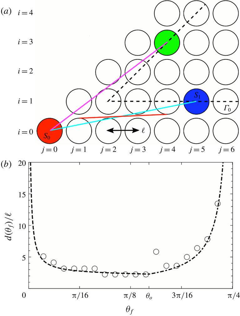
Hence we seek a model for the dependence of the distance
 $d$
between the sphere
 $S_{0}$
and the boundary
 $\unicode[STIX]{x1D6E4}_{0}$
as a function of
 $\unicode[STIX]{x1D703}_{f}$
when
 $\unicode[STIX]{x1D719}_{f}=0$
. Since
 ${\mathcal{W}}_{2D}^{S}$
,
 ${\mathcal{W}}_{2D}^{U}$
are material surfaces, a transverse connection occurs between manifolds which originate from spheres whose relative position vector is approximately parallel to the mean flow direction
 $\unicode[STIX]{x1D703}_{f}$
. Changes in the mean flow orientation can result in the destruction of existing connections between un/stable manifolds emanating from a pair of given spheres and the formation of new connections between other spheres pairs. This can lead to sudden fluctuations in
 $d$
and hence
 $\unicode[STIX]{x1D706}$
with changes in
 $\unicode[STIX]{x1D703}_{f}$
along
 $\unicode[STIX]{x1D719}_{f}=0$
, as shown in figure 12(c).
(a) Heteroclinic intersections in the BCC lattice for four different mean flow orientations
 $\unicode[STIX]{x1D703}_{f}$
(black arrow) with
 $\unicode[STIX]{x1D719}_{f}=0$
. The boundary
 $\unicode[STIX]{x1D6E4}_{0}$
(dashed line) is defined by the closest set of spheres
 $S_{1}$
which form heteroclinic intersections with the reference sphere
 $S_{0}$
. (b) Array of spheres (light grey (green online)) in
 $L_{Z}$
plane of the BCC lattice, with backward
 $\unicode[STIX]{x1D6FC}^{S}$
(dark grey (blue online)) and forward
 $\unicode[STIX]{x1D6FC}^{U}$
(light grey (red online)) streamlines emanating from spheres
 $S_{0}$
and
 $S_{1}$
respectively for various values of the flow orientations
 $\unicode[STIX]{x1D703}_{f}$
. Inset: bi-periodic cell of the
 $L_{Z}$
plane with the
 $\unicode[STIX]{x1D6FC}^{S}$
and
 $\unicode[STIX]{x1D6FC}^{U}$
streamlines shown for
 $(\unicode[STIX]{x1D703}_{f},\unicode[STIX]{x1D719}_{f})=(\unicode[STIX]{x03C0}/10,0)$
. (c) Forward
 $\unicode[STIX]{x1D6FC}^{U}$
and backward
 $\unicode[STIX]{x1D6FC}^{S}$
streamlines, emerging from
 $S_{0}$
and
 $S_{1}$
, respectively, for the mean flow direction
 $(\unicode[STIX]{x1D703}_{f},\unicode[STIX]{x1D719}_{f})=(\unicode[STIX]{x1D703}_{o},0)$
. The light grey (red online) and dark grey (blue online) arrows represent the respective directions in which
 $\unicode[STIX]{x1D6FC}^{U}$
and
 $\unicode[STIX]{x1D6FC}^{S}$
move with increasing
 $\unicode[STIX]{x1D703}_{f}$
. (d) Comparison between the normalised Lyapunov exponent
 $\unicode[STIX]{x1D706}(\unicode[STIX]{x1D703}_{f})/\langle \unicode[STIX]{x1D706}\rangle$
for the case
 $\unicode[STIX]{x1D719}_{f}=0$
in the BCC lattice from numerical simulations (filled circles), scaling
 $\unicode[STIX]{x1D706}\sim 1/d$
(empty circles), and predicted from (5.12) (dashed lines).
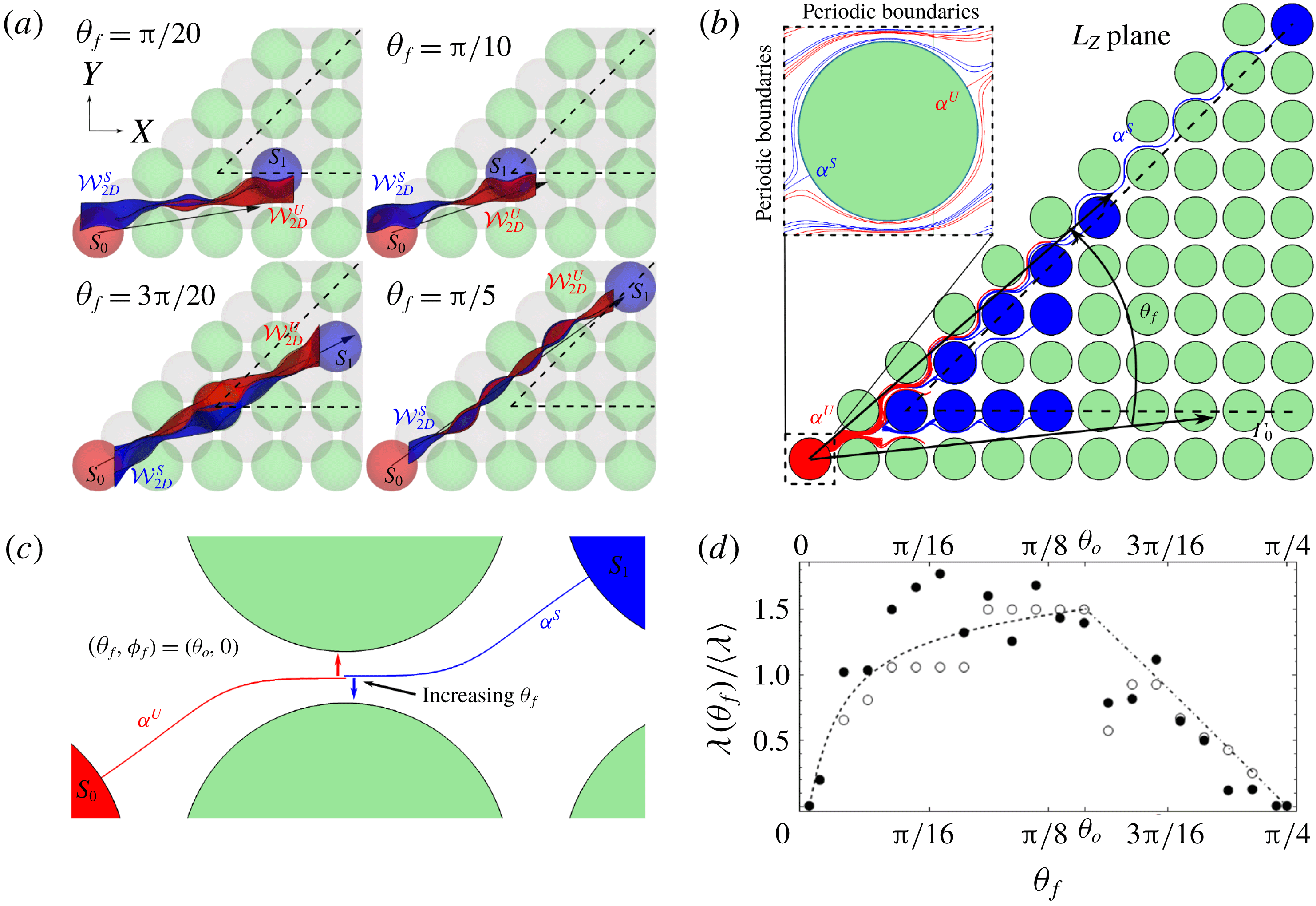
(a) Geometry of the BCC lattice for
 $\unicode[STIX]{x1D719}_{f}=0$
. Whilst the light grey (cyan online) line denotes the connection between the medium grey (red online) reference sphere
 $S_{0}$
and the dark grey (blue online) sphere on the lower branch of the boundary
 $\unicode[STIX]{x1D6E4}_{0}$
, the corresponding flow direction is indicated by the light grey (red online) straight line. In contrast, the light grey (green online) sphere on the upper branch of
 $\unicode[STIX]{x1D6E4}_{0}$
is connected with the reference sphere
 $S_{0}$
when the flow orientation is aligned with the purple line connecting the centres of the two spheres. (b) The approximate manifold distance
 $d(\unicode[STIX]{x1D703}_{f})$
(normalised by
 $\ell$
) as predicted by the lower (dashed) and upper (dot-dashed) curves as a function of the mean flow orientation
 $\unicode[STIX]{x1D703}_{f}$
, and numerical data (open circles).
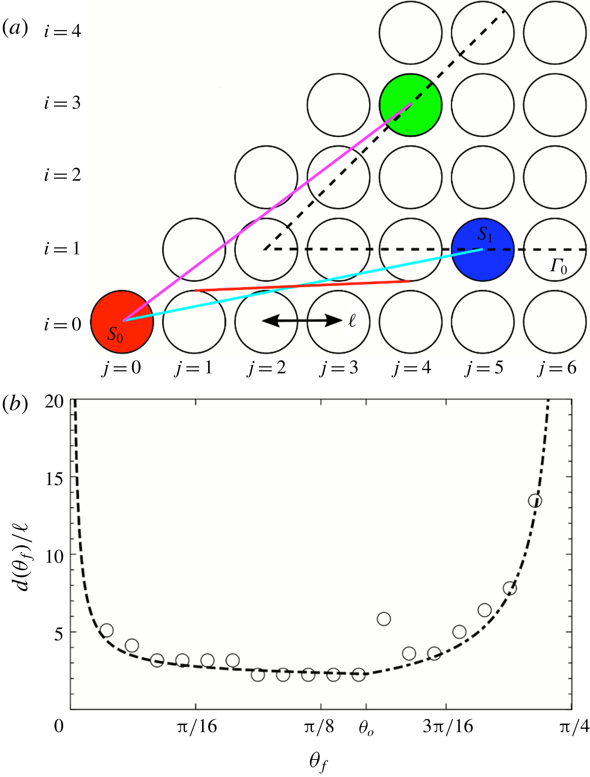
5.2 Geometric estimate of
 $d(\unicode[STIX]{x1D703}_{f})$
in the BCC lattice

To derive an estimate of
 $d(\unicode[STIX]{x1D703}_{f})$
, we consider geometric arguments based upon the boundary
 $\unicode[STIX]{x1D6E4}_{0}$
shown in figures 12(b), 13(a). We denote as
 $S_{1}$
the sphere nearest to the reference sphere
 $S_{0}$
for which a transverse heteroclinic intersection is possible for a given flow orientation
 $\unicode[STIX]{x1D703}_{f}$
(figure 12
a). As shown in figure 12(a), aside from a few exceptions (e.g.
 $\unicode[STIX]{x1D703}_{f}=3\unicode[STIX]{x03C0}/20$
), the sphere
 $S_{1}$
predominantly lies on the boundary
 $\unicode[STIX]{x1D6E4}_{0}$
, hence
 $\unicode[STIX]{x1D6E4}_{0}$
serves as an appropriate basis for the construction of a simple predictive model for
 $d(\unicode[STIX]{x1D703}_{f})$
.
For the BCC lattice, the spheres in the
 $L_{Z}$
plane have centres which lie at
 $(X,Y)=(\ell j,\ell i)$
for integers
 $j$
,
 $i$
, as shown in figure 13(a). The upper and lower branches of the boundary
 $\unicode[STIX]{x1D6E4}_{0}$
then correspond to
 $i=j-1$
,
 $i=1$
, respectively. Consequently the distance
 $d$
from the reference sphere
 $S_{0}$
to the boundaries
 $\unicode[STIX]{x1D6E4}_{0}$
expressed in terms of
 $j$
is
 $$\begin{eqnarray}\displaystyle & \displaystyle d_{upper}=\ell \sqrt{j^{2}+(j-1)^{2}}, & \displaystyle\end{eqnarray}$$
 $$\begin{eqnarray}\displaystyle & \displaystyle d_{lower}=\ell \sqrt{1+j^{2}}, & \displaystyle\end{eqnarray}$$
which respectively correspond to the purple and cyan lines shown in figure 13(a). It then remains to couch these expressions in terms of the flow orientation angle
 $\unicode[STIX]{x1D703}_{f}$
.
The orientation angle
 $\unicode[STIX]{x1D703}_{f}$
that corresponds to the transition between manifold intersections occurring between spheres located on the upper and lower branches of
 $\unicode[STIX]{x1D6E4}_{0}$
is denoted
 $\unicode[STIX]{x1D703}_{o}$
, where this orientation angle corresponds to the shortest distance
 $d$
and hence largest Lyapunov exponent for
 $\unicode[STIX]{x1D719}_{f}=0$
. At this transition (5.2), (5.3) must also satisfy
 $$\begin{eqnarray}\displaystyle d_{upper}|_{\unicode[STIX]{x1D703}_{f}=\unicode[STIX]{x1D703}_{o}}=d_{lower}|_{\unicode[STIX]{x1D703}_{f}=\unicode[STIX]{x1D703}_{o}}. & & \displaystyle\end{eqnarray}$$
As the
 $L_{Z}$
plane in which these spheres reside is a material plane, the streamlines
 $\unicode[STIX]{x1D6FC}^{S}$
,
 $\unicode[STIX]{x1D6FC}^{U}$
associated with the 2-D un/stable manifolds must deform around the spheres in
 $L_{Z}$
, as shown in figure 12(b). Due to such bending, the flow angle
 $\unicode[STIX]{x1D703}_{f}$
associated with a manifold connection
 $S_{0}$
and a sphere on the lower branch of
 $\unicode[STIX]{x1D6E4}_{0}$
is more accurately represented by a line tangent to the spheres immediately to the right of
 $S_{0}$
and left of the associated sphere in
 $\unicode[STIX]{x1D6E4}_{0}$
, of respective coordinates
 $(1,0)$
and
 $(j-1,1)$
, as indicated by the light grey (red online) line in figure 13(a).
If the angle of this line is given by the flow orientation
 $\unicode[STIX]{x1D703}_{f}$
, then the
 $(X,Y)$
coordinates of the tangent contact points at each end of the light grey (red online) line is then
 $$\begin{eqnarray}\displaystyle & \displaystyle (X_{1},Y_{1})=\left(\ell +\cos \left(\frac{\unicode[STIX]{x03C0}}{2}+\unicode[STIX]{x1D703}_{f}\right),\sin \left(\frac{\unicode[STIX]{x03C0}}{2}+\unicode[STIX]{x1D703}_{f}\right)\right), & \displaystyle\end{eqnarray}$$
 $$\begin{eqnarray}\displaystyle & \displaystyle (X_{2},Y_{2})=\left(\ell (j-1)+\cos \left(\frac{3\unicode[STIX]{x03C0}}{2}+\unicode[STIX]{x1D703}_{f}\right),\ell +\sin \left(\frac{3\unicode[STIX]{x03C0}}{2}+\unicode[STIX]{x1D703}_{f}\right)\right). & \displaystyle\end{eqnarray}$$
The slope of this line is then
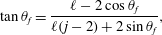 $$\begin{eqnarray}\displaystyle \tan \unicode[STIX]{x1D703}_{f}=\frac{\ell -2\cos \unicode[STIX]{x1D703}_{f}}{\ell (j-2)+2\sin \unicode[STIX]{x1D703}_{f}}, & & \displaystyle\end{eqnarray}$$
which yields the dependence of
 $j$
on
 $\unicode[STIX]{x1D703}_{f}$
on the lower branch of the boundary as
 $$\begin{eqnarray}\displaystyle j_{lower}(\unicode[STIX]{x1D703}_{f})=2+\cot \unicode[STIX]{x1D703}_{f}-\frac{2}{\ell \sin \unicode[STIX]{x1D703}_{f}}. & & \displaystyle\end{eqnarray}$$
Rather than constrain
 $j$
to integer values corresponding to sphere locations within the BCC lattice, we now consider
 $j$
as the set of real numbers
 $j\geqslant 1$
to yield a continuous set of flow angles
 $\unicode[STIX]{x1D703}_{f}$
. Substitution of (5.8) into (5.3) then yields a continuous estimate of
 $d(\unicode[STIX]{x1D703}_{f})$
for the lower boundary of
 $\unicode[STIX]{x1D6E4}_{0}$
, as
 $$\begin{eqnarray}\displaystyle d_{lower}(\unicode[STIX]{x1D703}_{f})=\ell \sqrt{1+\left(2+\cot \unicode[STIX]{x1D703}_{f}-\frac{2}{\ell \sin \unicode[STIX]{x1D703}_{f}}\right)^{2}}\quad \text{for }0<\unicode[STIX]{x1D703}_{f}\leqslant \unicode[STIX]{x1D703}_{o}. & & \displaystyle\end{eqnarray}$$
For manifold connections between the reference sphere
 $S_{0}$
and interaction spheres
 $S_{1}$
on the upper boundary of
 $\unicode[STIX]{x1D6E4}_{0}$
, the line which directly connects the centre of sphere
 $S_{0}$
to that of the corresponding sphere on the upper boundary of
 $\unicode[STIX]{x1D6E4}_{0}$
, shown by the purple line in figure 13(a), aligns closely with the corresponding flow orientation
 $\unicode[STIX]{x1D703}_{f}$
. From this there is a simple relationship between
 $j_{upper}$
and
 $\unicode[STIX]{x1D703}_{f}$
as
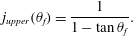 $$\begin{eqnarray}\displaystyle j_{upper}(\unicode[STIX]{x1D703}_{f})=\frac{1}{1-\tan \unicode[STIX]{x1D703}_{f}}. & & \displaystyle\end{eqnarray}$$
Again if we consider
 $j$
as a continuous rather than discrete variable, then by substituting this into (5.2) we obtain an expression for the distance from
 $S_{0}$
to the corresponding sphere on the upper boundary of
 $\unicode[STIX]{x1D6E4}_{0}$
as a function of flow orientation
 $\unicode[STIX]{x1D703}_{f}$
, as
 $$\begin{eqnarray}\displaystyle d_{upper}(\unicode[STIX]{x1D703}_{f})=\frac{\ell }{\cos \unicode[STIX]{x1D703}_{f}-\sin \unicode[STIX]{x1D703}_{f}}\quad \text{for }\unicode[STIX]{x1D703}_{o}<\unicode[STIX]{x1D703}_{f}\leqslant \unicode[STIX]{x03C0}/4. & & \displaystyle\end{eqnarray}$$
Combining (5.9), (5.11) the distance
 $d$
from the sphere
 $S_{0}$
to the boundary
 $\unicode[STIX]{x1D6E4}_{0}$
is
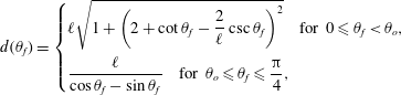 $$\begin{eqnarray}\displaystyle d(\unicode[STIX]{x1D703}_{f})=\left\{\begin{array}{@{}l@{}}\displaystyle \ell \sqrt{1+\left(2+\cot \unicode[STIX]{x1D703}_{f}-\frac{2}{\ell }\csc \unicode[STIX]{x1D703}_{f}\right)^{2}}\quad \text{for }0\leqslant \unicode[STIX]{x1D703}_{f}<\unicode[STIX]{x1D703}_{o},\\ \displaystyle \frac{\ell }{\cos \unicode[STIX]{x1D703}_{f}-\sin \unicode[STIX]{x1D703}_{f}}\quad \text{for }\unicode[STIX]{x1D703}_{o}\leqslant \unicode[STIX]{x1D703}_{f}\leqslant \frac{\unicode[STIX]{x03C0}}{4},\end{array}\right. & & \displaystyle\end{eqnarray}$$
where the transition angle
 $\unicode[STIX]{x1D703}_{o}\approx 0.46$
satisfies (5.4). This angle yields the minimum distance
 $d$
(and therefore the strongest chaotic mixing) and corresponds to the intersection of
 $\unicode[STIX]{x1D6FC}^{S}$
,
 $\unicode[STIX]{x1D6FC}^{U}$
shown in figure 12(c). As shown in figure 13(b), equation (5.12) corresponds very well with the distance as determined directly from the manifold intersections in the numerical simulations.
The scaling of the Lyapunov exponent with
 $\unicode[STIX]{x1D703}_{f}$
along the
 $\unicode[STIX]{x1D719}_{f}=0$
transect of the parameter space
 ${\mathcal{H}}$
shown in figure 3(b) is then obtained by combining (5.12) with the scaling of (5.1), which yields
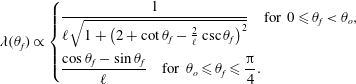 $$\begin{eqnarray}\displaystyle \unicode[STIX]{x1D706}(\unicode[STIX]{x1D703}_{f})\propto \left\{\begin{array}{@{}l@{}}\displaystyle \frac{1}{\ell \sqrt{1+\left(2+\cot \unicode[STIX]{x1D703}_{f}-\frac{2}{\ell }\csc \unicode[STIX]{x1D703}_{f}\right)^{2}}}\quad \text{for }0\leqslant \unicode[STIX]{x1D703}_{f}<\unicode[STIX]{x1D703}_{o},\\ \displaystyle \frac{\cos \unicode[STIX]{x1D703}_{f}-\sin \unicode[STIX]{x1D703}_{f}}{\ell }\quad \text{for }\unicode[STIX]{x1D703}_{o}\leqslant \unicode[STIX]{x1D703}_{f}\leqslant \frac{\unicode[STIX]{x03C0}}{4}.\end{array}\right. & & \displaystyle\end{eqnarray}$$
Normalising
 $\unicode[STIX]{x1D706}$
by
 $\langle \unicode[STIX]{x1D706}\rangle \equiv \int _{0}^{\unicode[STIX]{x03C0}/4}\unicode[STIX]{x1D706}(\unicode[STIX]{x1D703}_{f})\,\text{d}\unicode[STIX]{x1D703}_{f}$
, this simple predictive model (5.13) agrees quite well with the numerical data, as shown in figure 12(d). As expected, some discrepancies are observed due to (i) fluctuations in distance
 $d$
of manifold connections, and (ii) fluctuations in the fluid deformation across various manifold intersections. However, equation (5.13) does capture the gross trend of the Lyapunov exponent with
 $\unicode[STIX]{x1D703}_{f}$
, and in principle this geometric model could be extended to the BCC parameter space
 ${\mathcal{H}}$
, or more generally to the parameter space of any given lattice geometry, to predict the phase diagram of figure 3(b) more broadly. This could be achieved by identifying the governing symmetries that control mixing in a given periodic porous architecture, using these to construct an envelope similar to
 $\unicode[STIX]{x1D6E4}_{0}$
in figure 13, estimating the distance of that envelope to the reference sphere as a function of the flow orientation and then predicting the Lyapunov exponent distribution from the scaling (5.1). Conversely, the distribution of the Lyapunov exponent across the SC parameter space (figure 3
a) only exhibits weak deviations (
 $\unicode[STIX]{x1D706}\in [0,0.027]$
) from the completely regular dynamics
 $\unicode[STIX]{x1D706}=0$
at the boundaries of
 ${\mathcal{H}}$
due constraints imposed by reflection symmetries.
6 Conclusions
Fluid mixing of steady 3-D flows in topologically complex materials such as porous media is a problem of relevance to a wide variety of applications. For ordered media, the link between the microstructure, flow orientation and Lagrangian kinematics is not well understood, despite numerous applications in e.g. catalysis, chromatography and basic transport phenomena. In this paper we have used nonlinear dynamics, flow separation theory and symmetry analysis to uncover the mechanisms which control chaotic mixing in crystalline sphere arrays, an important class of discrete porous media. Specifically we have considered the Lagrangian kinematics of steady 3-D Stokes flow through close-packed SC and BCC lattices of uniform spheres, and connected the observed mixing dynamics to the geometry and inherent symmetries of the sphere lattices. As expected, breaking of reflection symmetries is a necessary condition for Lagrangian chaos due to the reversible nature of Stokes flow. Yet, an additional glide symmetry (comprised of a combined translation and reflection) is directly responsible for the creation of chaotic dynamics in the BCC lattice (Turuban et al. Reference Turuban, Lester, Borgne and Méheust2018), which contradicts long-held notions of symmetry breaking and the transition to chaos.
In this study we have extended the breadth and depth of the analysis in Turuban et al. (Reference Turuban, Lester, Borgne and Méheust2018) to (i) explain the fundamental differences between Lagrangian chaos in continuous and discrete porous media, and (ii) develop a predictive model for the Lyapunov exponent distribution over the mean flow orientation parameter space. Specifically, we have explained the mechanisms responsible for the generation of Lagrangian chaos in granular porous media. Similar to that of continuous media (Lester et al.
Reference Lester, Metcalfe and Trefry2013), the mechanisms in granular/discrete porous media revolve around the formation of transverse heteroclinic intersections between stable and unstable 2-D manifolds (respectively flow reattachment and separation surfaces) which originate from flow separation and reattachment in the skin friction field at the fluid/solid boundary. The nature of the skin friction field, the associated un/stable manifolds, their interactions and the resultant mixing dynamics are therefore dictated solely by the structure of the sphere lattices and the relative mean flow orientation. In particular, we have shown that the mixing dynamics of discrete porous media fundamentally differs from that of continuous porous media due to the point-wise nature of the grain contacts between particles. These singular contacts correspond to degenerate saddle points in the skin friction field, hence the topological complexity of discrete porous media is not sufficient to guarantee the formation of 2-D hyperbolic un/stable manifolds in the fluid interior. However, bifurcation of the skin friction field away from this state to admit non-degenerate saddle points can and does occur for discrete porous media, allowing flow separation by manifolds and the resulting chaotic advection. The fact that chaotic advection is inherent to continuous but not discrete porous media plays a significant role in the different degree of chaotic mixing observed in discrete (mean Lyapunov exponent
 $\langle \unicode[STIX]{x1D706}\rangle \approx 0.0760$
averaged over both the SC and BCC lattices, respectively, studied herein) and continuous (
 $\langle \unicode[STIX]{x1D706}\rangle \approx 0.1178$
in Lester et al. (Reference Lester, Metcalfe and Trefry2013)) porous media. These observations should also apply to natural (random) porous media, so that the rate of ergodic mixing (and hence, solute/scaler mixing) in natural granular media is expected to be less than that in porous networks.
In ordered granular media such as the sphere lattices investigated here, we find the Lagrangian kinematics is not only controlled by the solid phase geometry, but also by the orientation of the mean flow with respect to the granular lattice. The degree of Lagrangian chaos (as quantified via the mean Lyapunov exponent
 $\langle \unicode[STIX]{x1D706}\rangle$
) over the parameter space
 ${\mathcal{H}}$
of mean flow orientations for the SC (
 $\langle \unicode[STIX]{x1D706}\rangle \approx 0.0240$
) and BCC (
 $\langle \unicode[STIX]{x1D706}\rangle \approx 0.1280$
) lattices differ significantly from each other due to the differences in their symmetry space group, as discovered by Turuban et al. (Reference Turuban, Lester, Borgne and Méheust2018). We have uncovered the origins of chaotic mixing in this system, and based on the insights gained, we have inferred and verified from numerical data, that the Lyapunov exponent
 $\unicode[STIX]{x1D706}$
for a given flow orientation scales inversely with the shortest distance
 $d$
between spheres in the lattice that are connected via a transverse heteroclinic connection between un/stable 2-D manifolds emanating from these spheres. This observation has facilitated the derivation of an analytic model predicting the dependence of the Lyapunov exponent upon the mean flow orientation in the BCC lattice; the model agrees very well with direct numerical simulations. As this scaling
 $\unicode[STIX]{x1D706}\sim 1/d$
is expected to apply more broadly, we believe the approach developed to predict the Lyapunov exponent (namely via knowledge of the underlying symmetries of the microstructure and the manifold kinematics) may be successfully applied to chaotic mixing under steady flow conditions in other ordered 3-D systems.
Supplementary movies
Supplementary movies are available at https://doi.org/10.1017/jfm.2019.245.
Appendix A. Computation of Lyapunov exponents
Transverse Lyapunov exponents were computed via particle tracking in the simulated velocity fields. The computation starts with the advection of a set of particles which represents a material line (such that a line segment that spans adjacent particles approximates the true material line) that always lies in a plane transverse to the mean flow direction. Note that we use the subscript
 $1$
to denote the coordinate parallel to the mean flow direction, and the subscripts
 $2$
,
 $3$
for the transverse coordinates. Particles are advected over a fixed longitudinal offset
 $\unicode[STIX]{x0394}x_{1}$
via the explicit second-order scheme
 $$\begin{eqnarray}\displaystyle x_{j}(n+1)=x_{j}(n)+\unicode[STIX]{x0394}tv_{j}(n)+\frac{(\unicode[STIX]{x0394}t)^{2}}{2}\mathop{\sum }_{k=1}^{3}v_{k}(n)\unicode[STIX]{x2202}_{k}v_{j}(n), & & \displaystyle\end{eqnarray}$$
where the time step
 $\unicode[STIX]{x0394}t$
is computed as
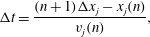 $$\begin{eqnarray}\displaystyle \unicode[STIX]{x0394}t=\frac{(n+1)\unicode[STIX]{x0394}x_{j}-x_{j}(n)}{v_{j}(n)}, & & \displaystyle\end{eqnarray}$$
where
 $v_{j}(n)$
is the longitudinal velocity of a given particle and
 $x_{j}(n)$
its longitudinal position in the previous iteration. This advection scheme does not allow for backward motion (
 $v_{j}\leqslant 0$
), so that in practice, we set a minimum threshold on particle longitudinal velocity below which the trajectory stops (
 $v_{j}=10^{-8}~\text{m}~\text{s}^{-1}$
). Results are not sensitive to the threshold value, since Stokes flow in a bead packing geometry is not prone to flow reversal.
The transverse elongation between two neighbouring particles
 $i$
and
 $i+1$
is then computed at each iteration as
 $$\begin{eqnarray}\displaystyle \unicode[STIX]{x1D70C}^{i}(n+1)=\unicode[STIX]{x1D70C}^{i}(n)\frac{|\boldsymbol{x}^{i}(n+1)-\boldsymbol{x}^{i+1}(n+1)|}{|\boldsymbol{x}^{i}(n)-\boldsymbol{x}^{i+1}(n)|}, & & \displaystyle\end{eqnarray}$$
where the norm
 $|\bullet |$
is the Euclidian distance in the transverse plane
 $(2,3)$
. When neighbouring particles in a line element get separated by more than a given distance (fixed to be
 $\unicode[STIX]{x1D6FF}l=5\times 10^{-5}d$
), refinement is achieved via insertion of a new particle in the middle of the line segment, and elongations are simply inherited from the original segment. The mean transverse stretching rate over a unit cell is then computed as
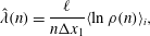 $$\begin{eqnarray}\displaystyle \hat{\unicode[STIX]{x1D706}}(n)=\frac{\ell }{n\unicode[STIX]{x0394}x_{1}}\langle \ln \unicode[STIX]{x1D70C}(n)\rangle _{i}, & & \displaystyle\end{eqnarray}$$
where
 $\ell =2d/\sqrt{3}$
,
 $d$
for the BCC and SC lattices respectively (
 $d$
being the diameter of a sphere), and the mean operator
 $\langle \bullet \rangle _{i}$
is defined as a weighted average with weight
 $\unicode[STIX]{x1D70C}_{i}^{-1}$
. Assuming the line segment aligns with the maximum stretching direction (which is a good approximation in the presence of exponential stretching), the mean stretching rate
 $\hat{\unicode[STIX]{x1D706}}(n)$
represents an average of the finite time Lyapunov exponent over the line element. Note
 $\hat{\unicode[STIX]{x1D706}}(n)$
has units of stretching per unit cell of the crystalline lattice rather stretching per unit time as is usual.
An estimate of the infinite time Lyapunov exponent
 $\tilde{\unicode[STIX]{x1D706}}$
for each flow orientation (averaged over the entire Poincaré section) is then given by advecting 100 randomly placed material lines downstream over large advection distances (approximately 30
 $d$
) and averaging the Lyapunov exponent over these cases as
 $$\begin{eqnarray}\displaystyle \tilde{\unicode[STIX]{x1D706}}=\langle \lim _{n\rightarrow \infty }\hat{\unicode[STIX]{x1D706}}(n)\rangle =\left\langle \lim _{n\rightarrow \infty }\frac{\ell }{n\unicode[STIX]{x0394}x_{1}}\langle \ln \unicode[STIX]{x1D70C}(n)\rangle _{i}\right\rangle . & & \displaystyle\end{eqnarray}$$
This method converges quickly and represents an average over about
 $10^{8}$
stretching values per flow orientation case.
Evolution of the stretching rate
 $\hat{\unicode[STIX]{x1D706}}$
along a given trajectory, as obtained by the method of Turuban et al. (Reference Turuban, Lester, Borgne and Méheust2018) (dark grey (blue online)) and that of the present study (light grey (orange online)).
 $\unicode[STIX]{x1D70F}_{a}$
is the mean advection time over a grain diameter (
 $\unicode[STIX]{x1D70F}_{a}=d/\bar{v}$
).
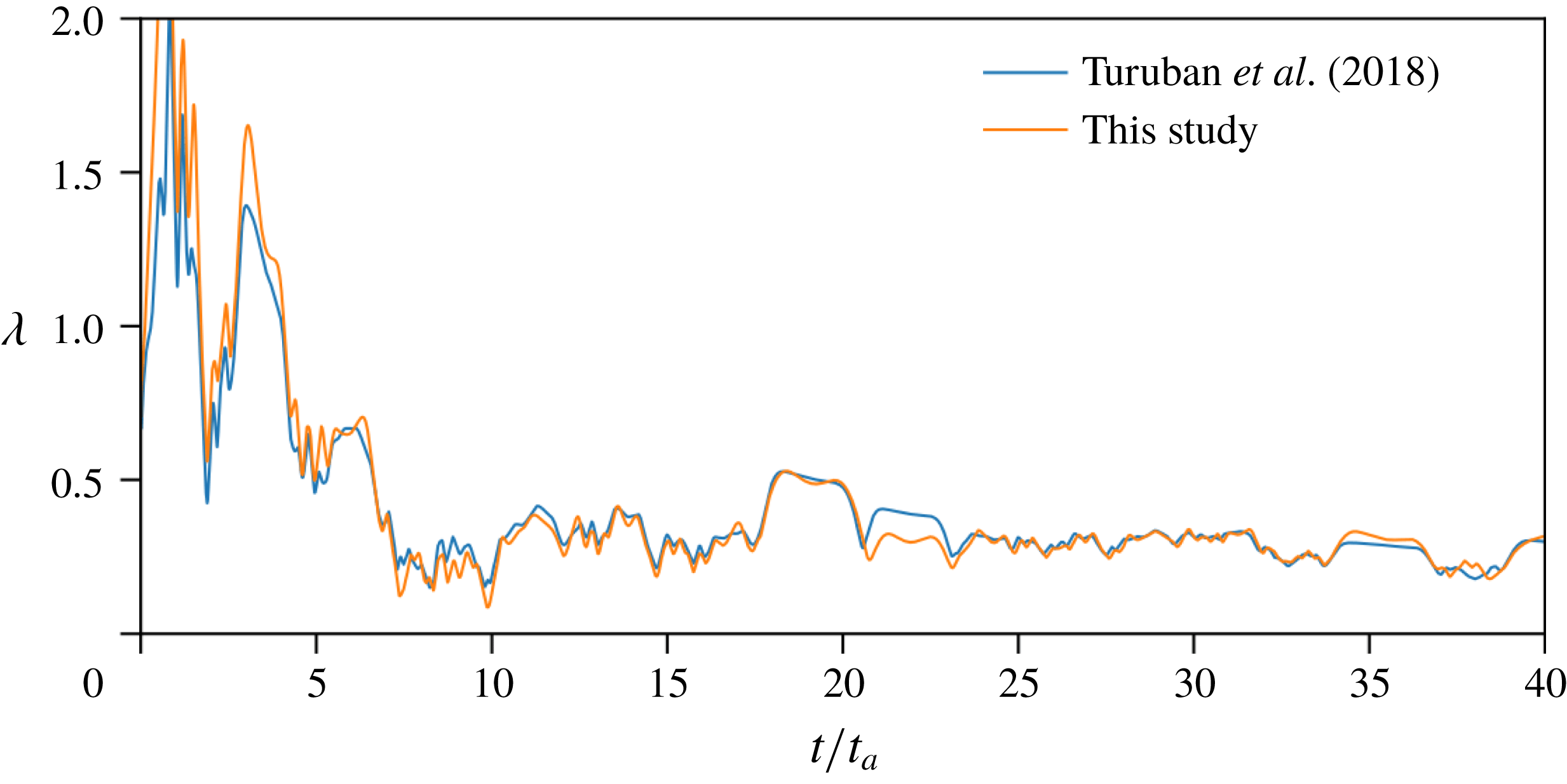
For validation, predictions of
 $\hat{\unicode[STIX]{x1D706}}(n)$
from (A 4) were compared with those given by the procedure used by Turuban et al. (Reference Turuban, Lester, Borgne and Méheust2018), which consisted in estimating the Lyapunov exponent (again taken as the average over the Poincaré map) of the long-time exponential growth rate of the largest eigenvalue
 $\unicode[STIX]{x1D708}(t)$
of the Cauchy–Green tensor
 $\unicode[STIX]{x1D63E}(\boldsymbol{X},t)$
. Turuban et al. (Reference Turuban, Lester, Borgne and Méheust2018) computed the velocity gradient tensor
 $\unicode[STIX]{x1D750}(\boldsymbol{X},t)=\unicode[STIX]{x1D735}_{\boldsymbol{x}}\boldsymbol{v}(\boldsymbol{X},t)$
in streamline coordinates, which renders
 $\unicode[STIX]{x1D750}(t)$
upper triangular (Lester et al.
Reference Lester, Dentz, Borgne and Barros2018) and significantly accelerates the convergence. Consistency between the two methods is illustrated in figure 14 which depicts the stretching rate
 $\hat{\unicode[STIX]{x1D706}}(n)$
via the two different methods along the same particle trajectory. For the sake of comparison, the present method has been modified to follow only two nearby particles whose mid point coincides with the given trajectory. Although small transient discrepancies in stretching rate
 $\hat{\unicode[STIX]{x1D706}}$
are expected due to the nature of the two methods, these give very close estimates of the average Lyapunov exponent
 $\tilde{\unicode[STIX]{x1D706}}$
.
Appendix B. Calculation of the Lyapunov exponent moments
$\langle \unicode[STIX]{x1D706}^{p}\rangle$

We define the
 $p$
th moment
 $\langle \unicode[STIX]{x1D706}^{p}\rangle$
of the Lyapunov exponent distribution
 $\unicode[STIX]{x1D706}(\unicode[STIX]{x1D703}_{f},\unicode[STIX]{x1D719}_{f})$
for the SC and BCC packings via the spherical surface integral
 $$\begin{eqnarray}\displaystyle \langle \unicode[STIX]{x1D706}^{p}\rangle =\frac{1}{4\unicode[STIX]{x03C0}}\int _{-\unicode[STIX]{x03C0}/2}^{\unicode[STIX]{x03C0}/2}\int _{-\unicode[STIX]{x03C0}}^{\unicode[STIX]{x03C0}}\unicode[STIX]{x1D706}(\unicode[STIX]{x1D703}_{f},\unicode[STIX]{x1D719}_{f})^{p}\cos \unicode[STIX]{x1D719}_{f}\,\text{d}\unicode[STIX]{x1D703}_{f}\,\text{d}\unicode[STIX]{x1D719}_{f}, & & \displaystyle\end{eqnarray}$$
where the parametric Lyapunov exponent distribution
 $\unicode[STIX]{x1D706}(\unicode[STIX]{x1D703}_{f},\unicode[STIX]{x1D719}_{f})$
is given over the parameter space
 ${\mathcal{H}}:(\unicode[STIX]{x1D703}_{f},\unicode[STIX]{x1D719}_{f},)=[\unicode[STIX]{x1D719}_{f},\unicode[STIX]{x03C0}/4]\times [0,\unicode[STIX]{x03C0}/4]$
as shown in figure 3. The
 $\cos \unicode[STIX]{x1D719}_{f}$
factor arises in (B 1) due to the non-uniform distribution of flow orientations with respect to the elevation angle
 $\unicode[STIX]{x1D719}_{f}$
, and is the reason why the
 $p$
th moment of
 $\unicode[STIX]{x1D706}$
over
 ${\mathcal{H}}$
is not necessarily equivalent to the same moment over the global domain
 ${\mathcal{H}}^{\ast }:(\unicode[STIX]{x1D703}_{f},\unicode[STIX]{x1D719}_{f})\in [-\unicode[STIX]{x03C0},\unicode[STIX]{x03C0}]\times [-\unicode[STIX]{x03C0}/2,\unicode[STIX]{x03C0}/2]$
. Below we describe a method to compute an estimate of
 $\langle \unicode[STIX]{x1D706}^{p}\rangle$
in (B 1) from values of
 $\unicode[STIX]{x1D706}$
in
 ${\mathcal{H}}$
. The
 $S_{1}^{m}$
and
 $S_{2}^{m}$
reflection symmetries inherent to both the SC and BCC packings allow the parameter space
 ${\mathcal{H}}$
to be extended to the subdomain
 ${\mathcal{H}}^{\prime }:(\unicode[STIX]{x1D703}_{f},\unicode[STIX]{x1D719}_{f})\in [0,\unicode[STIX]{x03C0}/2]\times [0,\unicode[STIX]{x03C0}/2]$
as shown in figure 15(a), which in turn can be extended to the full spherical domain
 ${\mathcal{H}}^{\ast }$
by translation of
 ${\mathcal{H}}^{\prime }$
. Due to these symmetries, the integral in (B 1) can be expanded to a series of integrals over the four regions shown on the left-hand side of figure 15(a) as
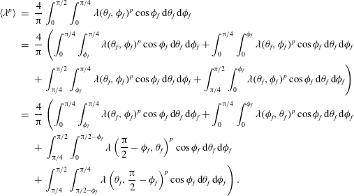 $$\begin{eqnarray}\displaystyle \langle \unicode[STIX]{x1D706}^{p}\rangle & = & \displaystyle \frac{4}{\unicode[STIX]{x03C0}}\int _{0}^{\unicode[STIX]{x03C0}/2}\int _{0}^{\unicode[STIX]{x03C0}/4}\unicode[STIX]{x1D706}(\unicode[STIX]{x1D703}_{f},\unicode[STIX]{x1D719}_{f})^{p}\cos \unicode[STIX]{x1D719}_{f}\,\text{d}\unicode[STIX]{x1D703}_{f}\,\text{d}\unicode[STIX]{x1D719}_{f}\nonumber\\ \displaystyle & = & \displaystyle \frac{4}{\unicode[STIX]{x03C0}}\left(\int _{0}^{\unicode[STIX]{x03C0}/4}\int _{\unicode[STIX]{x1D719}_{f}}^{\unicode[STIX]{x03C0}/4}\unicode[STIX]{x1D706}(\unicode[STIX]{x1D703}_{f},\unicode[STIX]{x1D719}_{f})^{p}\cos \unicode[STIX]{x1D719}_{f}\,\text{d}\unicode[STIX]{x1D703}_{f}\,\text{d}\unicode[STIX]{x1D719}_{f}+\int _{0}^{\unicode[STIX]{x03C0}/4}\int _{0}^{\unicode[STIX]{x1D719}_{f}}\unicode[STIX]{x1D706}(\unicode[STIX]{x1D703}_{f},\unicode[STIX]{x1D719}_{f})^{p}\cos \unicode[STIX]{x1D719}_{f}\,\text{d}\unicode[STIX]{x1D703}_{f}\,\text{d}\unicode[STIX]{x1D719}_{f}\right.\nonumber\\ \displaystyle & & \displaystyle +\left.\int _{\unicode[STIX]{x03C0}/4}^{\unicode[STIX]{x03C0}/2}\int _{\unicode[STIX]{x1D719}_{f}}^{\unicode[STIX]{x03C0}/4}\unicode[STIX]{x1D706}(\unicode[STIX]{x1D703}_{f},\unicode[STIX]{x1D719}_{f})^{p}\cos \unicode[STIX]{x1D719}_{f}\,\text{d}\unicode[STIX]{x1D703}_{f}\,\text{d}\unicode[STIX]{x1D719}_{f}+\int _{\unicode[STIX]{x03C0}/4}^{\unicode[STIX]{x03C0}/2}\int _{0}^{\unicode[STIX]{x1D719}_{f}}\unicode[STIX]{x1D706}(\unicode[STIX]{x1D703}_{f},\unicode[STIX]{x1D719}_{f})^{p}\cos \unicode[STIX]{x1D719}_{f}\,\text{d}\unicode[STIX]{x1D703}_{f}\,\text{d}\unicode[STIX]{x1D719}_{f}\right)\nonumber\\ \displaystyle & = & \displaystyle \frac{4}{\unicode[STIX]{x03C0}}\left(\int _{0}^{\unicode[STIX]{x03C0}/4}\int _{\unicode[STIX]{x1D719}_{f}}^{\unicode[STIX]{x03C0}/4}\unicode[STIX]{x1D706}(\unicode[STIX]{x1D703}_{f},\unicode[STIX]{x1D719}_{f})^{p}\cos \unicode[STIX]{x1D719}_{f}\,\text{d}\unicode[STIX]{x1D703}_{f}\,\text{d}\unicode[STIX]{x1D719}_{f}+\int _{0}^{\unicode[STIX]{x03C0}/4}\int _{0}^{\unicode[STIX]{x1D719}_{f}}\unicode[STIX]{x1D706}(\unicode[STIX]{x1D719}_{f},\unicode[STIX]{x1D703}_{f})^{p}\cos \unicode[STIX]{x1D719}_{f}\,\text{d}\unicode[STIX]{x1D703}_{f}\,\text{d}\unicode[STIX]{x1D719}_{f}\right.\nonumber\\ \displaystyle & & \displaystyle +\,\int _{\unicode[STIX]{x03C0}/4}^{\unicode[STIX]{x03C0}/2}\int _{0}^{\unicode[STIX]{x03C0}/2-\unicode[STIX]{x1D719}_{f}}\unicode[STIX]{x1D706}\left(\frac{\unicode[STIX]{x03C0}}{2}-\unicode[STIX]{x1D719}_{f},\unicode[STIX]{x1D703}_{f}\right)^{p}\cos \unicode[STIX]{x1D719}_{f}\,\text{d}\unicode[STIX]{x1D703}_{f}\,\text{d}\unicode[STIX]{x1D719}_{f}\nonumber\\ \displaystyle & & \displaystyle +\left.\int _{\unicode[STIX]{x03C0}/4}^{\unicode[STIX]{x03C0}/2}\int _{\unicode[STIX]{x03C0}/2-\unicode[STIX]{x1D719}_{f}}^{\unicode[STIX]{x03C0}/4}\unicode[STIX]{x1D706}\left(\unicode[STIX]{x1D703}_{f},\frac{\unicode[STIX]{x03C0}}{2}-\unicode[STIX]{x1D719}_{f}\right)^{p}\cos \unicode[STIX]{x1D719}_{f}\,\text{d}\unicode[STIX]{x1D703}_{f}\,\text{d}\unicode[STIX]{x1D719}_{f}\right).\end{eqnarray}$$
These integrals may then be simplified via a change of variables to yield an equation solely over the parameter space
 ${\mathcal{H}}$
as
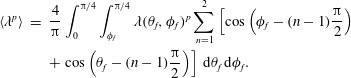 $$\begin{eqnarray}\displaystyle \langle \unicode[STIX]{x1D706}^{p}\rangle & = & \displaystyle \frac{4}{\unicode[STIX]{x03C0}}\int _{0}^{\unicode[STIX]{x03C0}/4}\int _{\unicode[STIX]{x1D719}_{f}}^{\unicode[STIX]{x03C0}/4}\unicode[STIX]{x1D706}(\unicode[STIX]{x1D703}_{f},\unicode[STIX]{x1D719}_{f})^{p}\mathop{\sum }_{n=1}^{2}\left[\cos \left(\unicode[STIX]{x1D719}_{f}-(n-1)\frac{\unicode[STIX]{x03C0}}{2}\right)\right.\nonumber\\ \displaystyle & & \displaystyle +\left.\cos \left(\unicode[STIX]{x1D703}_{f}-(n-1)\frac{\unicode[STIX]{x03C0}}{2}\right)\right]\,\text{d}\unicode[STIX]{x1D703}_{f}\,\text{d}\unicode[STIX]{x1D719}_{f}.\end{eqnarray}$$
Whilst this equation yields an estimate based on the entire Lyapunov exponent distribution
 $\unicode[STIX]{x1D706}$
within
 ${\mathcal{H}}$
, we only compute
 $\unicode[STIX]{x1D706}$
at discrete points
 $\unicode[STIX]{x1D706}_{i}\equiv \unicode[STIX]{x1D706}(\unicode[STIX]{x1D703}_{f,i},\unicode[STIX]{x1D719}_{f,i})$
as shown in figures 3 and 15(b). For these cases, a discrete analogue of (B 3) yields the estimate for the
 $p$
th moment as
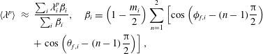 $$\begin{eqnarray}\displaystyle \langle \unicode[STIX]{x1D706}^{p}\rangle & {\approx} & \displaystyle \frac{\mathop{\sum }_{i}\unicode[STIX]{x1D706}_{i}^{p}\unicode[STIX]{x1D6FD}_{i}}{\mathop{\sum }_{i}\unicode[STIX]{x1D6FD}_{i}},\quad \unicode[STIX]{x1D6FD}_{i}=\left(1-\frac{m_{i}}{2}\right)\mathop{\sum }_{n=1}^{2}\left[\cos \left(\unicode[STIX]{x1D719}_{f,i}-(n-1)\frac{\unicode[STIX]{x03C0}}{2}\right)\right.\nonumber\\ \displaystyle & & \displaystyle +\left.\cos \left(\unicode[STIX]{x1D703}_{f,i}-(n-1)\frac{\unicode[STIX]{x03C0}}{2}\right)\right],\end{eqnarray}$$
where
 $m_{i}$
is the indicator function for points on the parameter space boundary
 $\unicode[STIX]{x2202}{\mathcal{H}}$
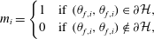 $$\begin{eqnarray}\displaystyle m_{i}=\left\{\begin{array}{@{}l@{}}1\quad \text{if }(\unicode[STIX]{x1D703}_{f,i},\unicode[STIX]{x1D703}_{f,i})\in \unicode[STIX]{x2202}{\mathcal{H}},\quad \\ 0\quad \text{if }(\unicode[STIX]{x1D703}_{f,i},\unicode[STIX]{x1D703}_{f,i})\notin \unicode[STIX]{x2202}{\mathcal{H}},\quad \end{array}\right. & & \displaystyle\end{eqnarray}$$
such that the factor
 $(1-m_{i}/2)$
in (B 4) ensures boundary points are not double counted during estimation of the moment
 $\langle \unicode[STIX]{x1D706}^{p}\rangle$
. From equation (B 4), the mean
 $\langle \unicode[STIX]{x1D706}\rangle$
and variance
 $\unicode[STIX]{x1D70E}_{\unicode[STIX]{x1D706}}^{2}=\langle \unicode[STIX]{x1D706}^{2}\rangle -\langle \unicode[STIX]{x1D706}\rangle ^{2}$
over
 ${\mathcal{H}}$
can be calculated. Figure 15(b) shows the same data as figure 3(a), but with a local colour scale to more clearly illustrate variability of the Lyapunov exponent in the SC packing.
(a) Tiling of the plane
 ${\mathcal{H}}^{\prime }:(\unicode[STIX]{x1D703},\unicode[STIX]{x1D719})\in [0,\unicode[STIX]{x03C0}/2]\times [0,\unicode[STIX]{x03C0}/2]$
with the parameter space
 ${\mathcal{H}}$
for the SC and BCC lattices. This subdomain
 ${\mathcal{H}}^{\prime }$
can then be extended to the full spherical domain
 ${\mathcal{H}}^{\ast }:(\unicode[STIX]{x1D703},\unicode[STIX]{x1D719})\in [-\unicode[STIX]{x03C0},\unicode[STIX]{x03C0}]\times [-\unicode[STIX]{x03C0}/2,\unicode[STIX]{x03C0}/2]$
by copying and translation. (b) Distribution of Lyapunov exponent over mean flow orientation space
 ${\mathcal{H}}$
for SC lattice (same as for figure 3
a) with local colour scale to more clearly illustrate the local Lyapunov exponent distribution.