2 Mathematical model for a buoyancy-driven hydraulic fracture with solidification

This section outlines the mathematical model for a magma ascent in a vertical crack, in which the effects of magma viscosity, rock toughness and magma solidification on fracture walls are considered. Assuming a line source, which is commonly the case in the analysis of buoyancy-driven fractures (Spence et al. 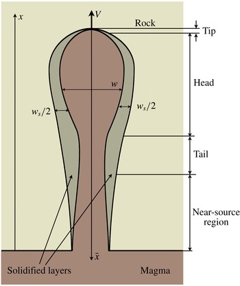Reference Spence, Sharp and Turcotte1987; Lister Reference Lister1990; Roper & Lister Reference Roper and Lister2007), the problem can be treated assuming that a fracture propagates in the vertical $x$ direction under plane-strain-elastic conditions; see figure 1. In this case, the conservation of mass can be written as

(2.1) $$\begin{eqnarray}{\displaystyle \frac{1}{{\it\rho}_{m}}}{\displaystyle \frac{\partial ({\it\rho}_{m}w+{\it\rho}_{s}w_{s})}{\partial t}}+{\displaystyle \frac{\partial q_{x}}{\partial x}}=0,\end{eqnarray}$$

where $w$ is the portion of the fracture width occupied by a liquid magma, $w_{s}$ is the portion of the fracture width occupied by a solidified magma, ${\it\rho}_{m}$ is the mass density of the liquid magma, ${\it\rho}_{s}$ is the mass density of the solid magma and $q_{x}$ is the magma flux. By treating magma as a Newtonian fluid, the flux can be calculated based on a Poiseuille flow solution as

(2.2) $$\begin{eqnarray}q_{x}=-{\displaystyle \frac{w^{3}}{{\it\mu}^{\prime }}}\left({\displaystyle \frac{\partial p}{\partial x}}-{\rm\Delta}{\it\rho}g\right).\end{eqnarray}$$

Figure 1.

Schematics of a buoyancy-driven hydraulic fracture in a rock propagating from a magma chamber.

Here, ${\it\mu}^{\prime }=12{\it\mu}_{f}$ , and ${\it\mu}_{f}$ is the magma viscosity, $p(x)$ is the magma pressure, ${\rm\Delta}{\it\rho}={\it\rho}_{r}-{\it\rho}_{m}$ is the difference between the mass densities of rock and liquid magma, while $g$ is the gravitational constant. The term ${\rm\Delta}{\it\rho}g$ in (2.2) captures the effect of buoyancy, which is the primary driving force for buoyancy-driven hydraulic fractures (see, e.g., Lister (Reference Lister1990), Roper & Lister (Reference Roper and Lister2007)). Assuming that the fracture originates from a pressurized magma chamber whose boundary is traction-free, the elasticity equation that relates the magma pressure to the total fracture width in plane-strain conditions (see, e.g., Broberg (Reference Broberg1999), Roper & Lister (Reference Roper and Lister2005)) can be written as

(2.3) $$\begin{eqnarray}p=-{\displaystyle \frac{E^{\prime }}{4{\rm\pi}}}\int _{0}^{l}{\displaystyle \frac{\partial (w+w_{s})}{\partial s}}\left[{\displaystyle \frac{1}{s-x}}-{\displaystyle \frac{s^{2}-4sx-x^{2}}{(s+x)^{3}}}\right]\,\text{d}s,\end{eqnarray}$$

where $E^{\prime }=E/(1-{\it\nu}^{2})$ is the plane-strain Young’s modulus. The first part of the integral kernel represents the solution for an infinite crack geometry, while the second term ensures the traction-free boundary condition at $x=0$ . By focusing on relatively long fractures, for which the effect of free surface can be neglected, (2.3) reduces to

(2.4) $$\begin{eqnarray}p=-{\displaystyle \frac{E^{\prime }}{4{\rm\pi}}}\int _{-\infty }^{l}{\displaystyle \frac{\partial (w+w_{s})}{\partial s}}{\displaystyle \frac{1}{s-x}}\,\text{d}s.\end{eqnarray}$$

The propagation condition at the fracture tip comes from a linear elastic fracture mechanics (LEFM) analysis (Irwin Reference Irwin1957; Rice Reference Rice and Liebowitz1968), and states that

(2.5) $$\begin{eqnarray}w\rightarrow {\displaystyle \frac{K^{\prime }}{E^{\prime }}}(l-x)^{1/2},\quad x\rightarrow l,\end{eqnarray}$$

where $K^{\prime }=8K_{Ic}/\sqrt{2{\rm\pi}}$ is the scaled fracture toughness and $l$ is the length of the fracture. Finally, one needs to couple the hydro-mechanical problem with the thermal problem that accounts for magma solidification. By assuming that the fracture propagates monotonically (i.e. the fracture does not recede by complete solidification of the tip) and that the temperature of the magma is equal to the solidification temperature, analysis of a one-dimensional heat transfer problem in the direction perpendicular to the fracture (Carslaw & Jaeger Reference Carslaw and Jaeger1959; Bolchover & Lister Reference Bolchover and Lister1999) leads to

(2.6) $$\begin{eqnarray}w_{s}=4{\it\lambda}\sqrt{{\it\kappa}}\sqrt{t-t_{0}(x)}={\it\alpha}\sqrt{t-t_{0}(x)},\end{eqnarray}$$

where ${\it\kappa}$ is the thermal diffusivity of rock (the thermal diffusivity of solidified magma is assumed to be the same), $t_{0}(x)$ signifies the time instant at which the fracture front was located at a given point $x$ and ${\it\lambda}$ is a constant that is calculated from

(2.7) $$\begin{eqnarray}{\rm\pi}^{1/2}{\it\lambda}\text{e}^{{\it\lambda}^{2}}\text{erfc}(-{\it\lambda})={\displaystyle \frac{C_{p}(T_{s}-T_{\infty })}{L_{m}}}.\end{eqnarray}$$

Here, $C_{p}$ is the specific heat of the solidified magma, $T_{s}$ is the solidification temperature, $T_{\infty }$ is the rock temperature away from the dike and $L_{m}$ is the specific latent heat of magma solidification. It should be noted that (2.6) accounts for a factor of two, which reflects the fact that there are two layers that grow on each side of the fracture. According to Wilson & Head (Reference Wilson, Head, Smellie and Chapman2002), the properties of magma are ${\it\kappa}=10^{-6}~\text{m}^{2}~\text{s}^{-1}$ , $L_{m}=2.09\times 10^{5}~\text{J}~\text{kg}^{-1}$ and $C_{p}=1200~\text{J}~\text{kg}^{-1}~\text{K}^{-1}$ . Assuming a wide range of temperature difference $1\lesssim T_{s}-T_{\infty }^{\infty }\lesssim 10^{3}$  K, the range of values of ${\it\lambda}$ is relatively narrow, $2\times 10^{-3}\lesssim {\it\lambda}\lesssim 0.2$ . In this case, the range for ${\it\alpha}$ is $10^{-5}\lesssim {\it\alpha}\lesssim 10^{-3}~\text{m}~\text{s}^{-1/2}$ .

It should be noted that the time dependence in (2.6) is identical to that for the problem of fluid leak-off from a hydraulic fracture to porous rock, which is typically modelled by Carter’s model (Carter Reference Carter, Howard and Fast1957). While there are some differences in the analyses, this is still not surprising, since the diffusion equation is used in both approaches. As for Carter’s leak-off model, (2.6) is valid in situations when the thermal diffusion length scale is much smaller than the fracture length. Given that magma dikes are typically a few kilometres long, while the length scale of thermal penetration is unlikely to substantially exceed a metre scale ( $t=d^{2}/{\it\kappa}\approx 10$  days assuming thermal diffusivity of rock ${\it\kappa}=10^{-6}~\text{m}^{2}~\text{s}^{-1}$ and $d=1$  m), the one-dimensional model (2.6) is expected to produce accurate results in most cases.

The buoyancy-driven fracture can be divided into several regions: the tip region, the head region, the tail region and the near-source region; see figure 1. The tip region can be loosely defined as a small region near the tip, whose length is much smaller than the head size. Fracture toughness, magma viscosity and solidification (but not buoyancy) compete to determine the behaviour in the tip region. The head region corresponds to the part of the fracture in which the fracture width has a local maximum, and where the buoyancy starts to play a crucial role. It should be noted that Roper & Lister (Reference Roper and Lister2007) also defined additional regions in between the head and the tail, which are not that important for the current formulation, and can be moved to either the head or the tail region. The tail region occurs after the head. The elastic interactions become less important in the tail region, and its shape is mainly determined by the balance of buoyancy pressure gradient, viscous forces and the solidification rate. If a finite fracture is considered, it is also necessary to introduce a near-source region located near the magma chamber, in which the elastic effects of the free surface play an important role. It is also crucial to note that the ambient temperature of the rock, $T_{\infty }$ , is in general a function of $x$ , since the rock is warmer near the magma chamber and the temperature decreases further away from it. For this reason, it is expected that there is no solidification at the magma chamber boundary, and the solidification in the near-source region is small, as schematically indicated in figure 1.

To simplify the problem, further analysis in this paper is focused on the propagation of a semi-infinite buoyancy-driven hydraulic fracture, in which case the near-source region is of little importance. Such a simplification allows us to describe the tip, the head and the tail regions in great detail. In addition, it is assumed that $T_{\infty }=\text{const}.$ , and hence ${\it\alpha}=\text{const}.$ , in which case a steady solution can be analysed.

3 Problem formulation for a semi-infinite fracture

This section formulates the problem for the steady propagation of a buoyancy-driven hydraulic fracture with solidification, which is modelled according to the description in § 2. To this end, let us assume that the fracture propagates steadily with a velocity $V$ , in which case it is useful to introduce a new moving spatial coordinate that originates at the fracture tip and increases towards the rest of the fracture, i.e. $\bar{x}=Vt-x$ ; see figure 1. Since we are looking for a steady solution, the fracture width and pressure become functions of $\bar{x}$ only. In this situation, by changing variables in (2.1) and integrating the result, one has

(3.1) $$\begin{eqnarray}wV+{\displaystyle \frac{{\it\rho}_{s}}{{\it\rho}_{m}}}w_{s}V-q_{x}=0.\end{eqnarray}$$

The expression for the fluid flux (2.2) transforms into

(3.2) $$\begin{eqnarray}q_{x}={\displaystyle \frac{w^{3}}{{\it\mu}^{\prime }}}\left({\displaystyle \frac{\partial p}{\partial \bar{x}}}+{\rm\Delta}{\it\rho}g\right),\end{eqnarray}$$

while the width of the solidified magma (2.6) becomes

(3.3) $$\begin{eqnarray}w_{s}={\it\alpha}\sqrt{{\displaystyle \frac{\bar{x}}{V}}}.\end{eqnarray}$$

It should be noted that the above equation is obtained from (2.6) by substituting $t_{0}=t-\bar{x}/V$ , where $\bar{x}=0$ corresponds to the tip of the fracture. The elasticity equation (2.4), reduced to a semi-infinite fracture, can be inverted (Garagash & Detournay Reference Garagash and Detournay2000; Garagash et al. Reference Garagash, Detournay and Adachi2011) to obtain

(3.4) $$\begin{eqnarray}w+w_{s}={\displaystyle \frac{K^{\prime }}{E^{\prime }}}\bar{x}^{1/2}+{\displaystyle \frac{4}{{\rm\pi}E^{\prime }}}\int _{0}^{\infty }K(\bar{x},\bar{s})p(\bar{s})\,\text{d}\bar{s},\end{eqnarray}$$

where the kernel is given by

(3.5) $$\begin{eqnarray}K(\bar{x},\bar{s})=\ln \left|{\displaystyle \frac{\bar{x}^{1/2}+\bar{s}^{1/2}}{\bar{x}^{1/2}-\bar{s}^{1/2}}}\right|-2{\displaystyle \frac{\bar{x}^{1/2}}{\bar{s}^{1/2}}}.\end{eqnarray}$$

The advantage of the inversion (3.4) in lieu of the classical inversion formula (Rice Reference Rice and Liebowitz1968) lies in capturing the boundary condition at the tip (2.5) automatically, and the extended validity region of the inversion. By following the analysis in Dontsov & Peirce (Reference Dontsov and Peirce2015), integration by parts can be employed to rewrite (3.4) as

(3.6) $$\begin{eqnarray}w+w_{s}={\displaystyle \frac{K^{\prime }}{E^{\prime }}}\bar{x}^{1/2}-{\displaystyle \frac{4}{{\rm\pi}E^{\prime }}}\int _{0}^{\infty }F(\bar{x},\bar{s}){\displaystyle \frac{\text{d}p}{\text{d}\bar{s}}}\,\text{d}\bar{s},\end{eqnarray}$$

where the new kernel is given by

(3.7a,b ) $$\begin{eqnarray}K(\bar{x},\bar{s})={\displaystyle \frac{\partial F(\bar{x},\bar{s})}{\partial \bar{s}}},\quad F(\bar{x},\bar{s})=(\bar{s}-\bar{x})\ln \left|{\displaystyle \frac{\bar{x}^{1/2}+\bar{s}^{1/2}}{\bar{x}^{1/2}-\bar{s}^{1/2}}}\right|-2\bar{x}^{1/2}\bar{s}^{1/2}.\end{eqnarray}$$

By combining (3.1)–(3.3), and substituting the pressure gradient into (3.6), we have

(3.8) $$\begin{eqnarray}w(\bar{x})=\left({\displaystyle \frac{K^{\prime }}{E^{\prime }}}-{\displaystyle \frac{{\it\alpha}}{V^{1/2}}}\right)\bar{x}^{1/2}-{\displaystyle \frac{4}{{\rm\pi}E^{\prime }}}\int _{0}^{\infty }F(\bar{x},\bar{s})\left\{{\displaystyle \frac{{\it\mu}^{\prime }}{w(\bar{s})^{2}}}\left[V+{\displaystyle \frac{{\it\rho}_{s}{\it\alpha}V^{1/2}}{{\it\rho}_{m}}}{\displaystyle \frac{\bar{s}^{1/2}}{w}}\right]-{\rm\Delta}{\it\rho}g\right\}\,\text{d}\bar{s}.\end{eqnarray}$$

Finally, by introducing the dimensionless quantities

(3.9a-e ) $$\begin{eqnarray}\tilde{w}={\displaystyle \frac{w}{{\it\gamma}\bar{x}^{1/2}}},\quad {\it\chi}={\displaystyle \frac{{\it\rho}_{s}{\it\alpha}}{{\it\rho}_{m}V^{1/2}{\it\gamma}}},\quad \tilde{g}={\displaystyle \frac{{\rm\Delta}{\it\rho}gL^{3/2}}{{\it\gamma}E^{\prime }}},\quad \tilde{x}=\left({\displaystyle \frac{\bar{x}}{L}}\right)^{1/2},\quad \tilde{s}=\left({\displaystyle \frac{\bar{s}}{L}}\right)^{1/2},\end{eqnarray}$$

where

(3.10a,b ) $$\begin{eqnarray}{\it\gamma}={\displaystyle \frac{K^{\prime }}{E^{\prime }}}-{\displaystyle \frac{{\it\alpha}}{V^{1/2}}},\quad L=\left({\displaystyle \frac{{\it\gamma}^{3}E^{\prime }}{{\it\mu}^{\prime }V}}\right)^{2},\end{eqnarray}$$

equation (3.8) can be further reduced to

(3.11) $$\begin{eqnarray}\tilde{w}(\tilde{x})=1+{\displaystyle \frac{8}{{\rm\pi}}}\int _{0}^{\infty }G(\tilde{s}/\tilde{x})\left[{\displaystyle \frac{1}{\tilde{w}(\tilde{s})^{2}}}+{\displaystyle \frac{{\it\chi}}{\tilde{w}(\tilde{s})^{3}}}-\tilde{g}\tilde{s}^{2}\right]\,\text{d}\tilde{s},\end{eqnarray}$$

where the kernel is

(3.12a-c ) $$\begin{eqnarray}G(t)={\displaystyle \frac{1-t^{2}}{t}}\ln \left|{\displaystyle \frac{1+t}{1-t}}\right|+2,\quad G(0)=4,\quad G(t)\approx {\displaystyle \frac{4}{3t^{2}}},\quad t\gg 1.\end{eqnarray}$$

It should be noted that the procedure for obtaining (3.11) is very similar to the analysis in Dontsov & Peirce (Reference Dontsov and Peirce2015), in which a problem of buoyancy-driven hydraulic fracture without solidification was analysed. The primary advantage of (3.11) is that the whole problem is rewritten in terms of one non-singular integral equation (the function $G(t)$ in (3.12) is not singular). This greatly reduces the complexity of the problem and permits us to obtain an accurate solution using standard numerical techniques. It should also be noted that the width of the solidified layer (3.3), written in terms of the scaling (3.9), is

(3.13) $$\begin{eqnarray}\tilde{w}_{s}={\displaystyle \frac{{\it\rho}_{m}}{{\it\rho}_{s}}}{\it\chi}.\end{eqnarray}$$

It is interesting to note that the presence of solidification (as compared with a buoyancy-driven fracture without solidification) adds an additional term in (3.11) that is proportional to ${\it\chi}$ , and effectively decreases the value of the fracture toughness through ${\it\gamma}$ . In addition, there is no steady solution for ${\it\gamma}<0$ , which introduces a minimum velocity for a steady solution as

(3.14) $$\begin{eqnarray}V_{\mathit{min}}=\left({\displaystyle \frac{{\it\alpha}E^{\prime }}{K^{\prime }}}\right)^{2},\end{eqnarray}$$

which was also mentioned in Bolchover & Lister (Reference Bolchover and Lister1999).

By taking ${\it\alpha}=O(10^{-4})~\text{m}~\text{s}^{-1/2}$ , $E^{\prime }=O(10^{10})$ Pa and $K^{\prime }=O(10^{6})~\text{Pa}~\text{m}^{1/2}$ , it becomes clear that the minimum velocity can be of the order of $1~\text{m}~\text{s}^{-1}$ .

The integral equation (3.11) has four terms on the right-hand side. The first term (which is equal to one) reflects the effect of fracture toughness. The second term (i.e. the first term under the integral sign) captures the effect of fluid viscosity. The third term (which is proportional to ${\it\chi}$ ) captures the effect of solidification, while the last term (proportional to $\tilde{g}$ ) describes the effect of buoyancy. In this situation, the integral equation (3.11) can be understood as

(3.15) $$\begin{eqnarray}\tilde{w}~\text{`}=\text{'}~\tilde{w}_{k}~\text{`}+\text{'}~\tilde{w}_{m}~\text{`}+\text{'}~\tilde{w}_{\tilde{m}}~\text{`}+\text{'}~\tilde{w}_{g},\end{eqnarray}$$

where the summation does not represent actual mathematical summation, but states that the solution (left-hand side) is influenced by the interplay between fracture toughness, viscosity, solidification (leak-off) and gravity (buoyancy). It can happen that only one term dominates the response, or multiple terms have influences that are comparable in magnitude. In order to understand the influence of each term, § 4 considers the limiting solutions of (3.11). Then, § 5 analyses transitions from one limiting solution to another, which occur when two out of the four terms in (3.15) have similar magnitudes. Finally, §§ 6 and 7 focus on more general cases, when three or four terms in (3.15) interplay to provide a solution.

It should be noted here that the case $\tilde{g}=0$ corresponds to a semi-infinite hydraulic fracture with leak-off (here the solidification is mathematically analogous to leak-off). This problem was first analysed in Garagash et al. (Reference Garagash, Detournay and Adachi2011) and then revisited in Dontsov & Peirce (Reference Dontsov and Peirce2015), where a non-singular integral equation formulation (similar to (3.11)) was used. For this reason, it is natural to expect that the tip region of the buoyancy-driven hydraulic fracture under consideration would behave in accordance with the analysis in Garagash et al. (Reference Garagash, Detournay and Adachi2011) and Dontsov & Peirce (Reference Dontsov and Peirce2015). Moreover, due to the mathematical analogy, the terms ‘solidification’ and ‘leak-off’ will be used interchangeably throughout the paper. The problem with ${\it\chi}=0$ (and $\tilde{g}\neq 0$ ) has been analysed in a series of papers (see, e.g., Spence et al. (Reference Spence, Sharp and Turcotte1987), Lister (Reference Lister1990), Roper & Lister (Reference Roper and Lister2007)), and then also revisited in Dontsov & Peirce (Reference Dontsov and Peirce2015) by way of a non-singular integral equation formulation. This study, however, aims to consider a general case of ${\it\chi}\neq 0$ and $\tilde{g}\neq 0$ . Despite many similarities between this study and previous analyses (Roper & Lister Reference Roper and Lister2007; Garagash et al. Reference Garagash, Detournay and Adachi2011), we adopt a notation that is consistent with the integral formulation (3.11), which is similar to, but not identical to, the one used in prior studies.

A numerical solution of the integral equation (3.11) (or similar equations) is used in §§ 4–7. A relatively straightforward numerical algorithm is used to obtain a solution, since the latter integral equation has a non-singular kernel. A spatial grid of points distributed uniformly on a logarithmic scale is used to effectively capture the near-tip behaviour, while Simpson’s rule is used to discretize the integral and Newton’s method is used to solve the system of nonlinear algebraic equations. This approach is proven to converge rapidly and to provide accurate results even on relatively coarse meshes (Dontsov & Peirce Reference Dontsov and Peirce2015). It should be noted that the use of a logarithmic scale is equivalent to a change of variable $\tilde{s}=\text{e}^{{\hat{s}}}$ ( ${\hat{s}}$ is discretized on a linear scale), in which case the integral becomes a convolution.

4 Limiting solutions

Let us first recall the so-called vertex solutions (Garagash et al. Reference Garagash, Detournay and Adachi2011), which occur when $\tilde{g}=0$ . In the latter situation, the right-hand side of (3.11) features three terms. If the first term dominates, then

(4.1) $$\begin{eqnarray}\tilde{w}_{k}=1,\end{eqnarray}$$

which is referred to as the toughness solution. This solution appears when the effects of solidification (leak-off) and viscosity are negligible compared with the fracture toughness. In this case, the scaled width is constant, but the real fracture width increases as $\bar{x}^{1/2}$ away from the tip; see (3.9). When the second term in (3.11) dominates, then

(4.2) $$\begin{eqnarray}\tilde{w}_{m}(\tilde{x})={\displaystyle \frac{8}{{\rm\pi}}}\int _{0}^{\infty }{\displaystyle \frac{G(\tilde{s}/\tilde{x})}{\tilde{w}_{m}(\tilde{s})^{2}}}\,\text{d}\tilde{s}~\Longrightarrow ~\tilde{w}_{m}={\it\beta}_{m}\tilde{x}^{1/3},\quad {\it\beta}_{m}=2^{1/3}3^{5/6},\end{eqnarray}$$

where the following integral has been used:

(4.3) $$\begin{eqnarray}\int _{0}^{\infty }{\displaystyle \frac{G(t)}{t^{p}}}\,\text{d}t={\displaystyle \frac{2{\rm\pi}}{p(2-p)}}\tan \left({\displaystyle \frac{{\rm\pi}}{2}}p\right)\end{eqnarray}$$

for $-1<p<1$ (the integral does not converge for values of $p$ that are outside this interval). The solution $\tilde{w}_{m}$ is referred to as the viscous solution, and occurs when the fluid viscosity dominates the response. It should be noted that the real width increases away from the tip as $\bar{x}^{2/3}$ . When the third term in (3.11) dominates the response, then

(4.4) $$\begin{eqnarray}\tilde{w}_{\tilde{m}}(\tilde{x})={\displaystyle \frac{8}{{\rm\pi}}}\int _{0}^{\infty }G(\tilde{s}/\tilde{x}){\displaystyle \frac{{\it\chi}}{\tilde{w}_{\tilde{m}}(\tilde{s})^{3}}}\,\text{d}\tilde{s}~\Longrightarrow ~\tilde{w}_{\tilde{m}}={\it\beta}_{\tilde{m}}{\it\chi}^{1/4}\tilde{x}^{1/4},\quad {\it\beta}_{\tilde{m}}={\displaystyle \frac{4}{15^{1/4}(\sqrt{2}-1)^{1/4}}}.\end{eqnarray}$$

The solution $\tilde{w}_{\tilde{m}}$ is called the leak-off solution (again, solidification and leak-off are mathematically equivalent), and the real width increases away from the tip as $\bar{x}^{5/8}$ .

The vertex solutions $\tilde{w}_{k}$ , $\tilde{w}_{m}$ and $\tilde{w}_{\tilde{m}}$ are the asymptotic solutions of (3.11), which means that they are actual solutions for some limiting conditions. For the case of buoyancy-driven fracture, such asymptotic solutions appear at the fracture tip at length scales much smaller than the size of the fracture head; see figure 1. There is no similar asymptotic solution related to the gravitational term in (3.11). Instead, this term introduces a length scale that determines the size of the head. In order to quantify the effect of gravity on the transition from the tip region to the head, it is useful to quantify the effect of gravity as

(4.5) $$\begin{eqnarray}\tilde{w}_{g}=-{\displaystyle \frac{8}{{\rm\pi}}}\int _{0}^{\tilde{x}}G(\tilde{s}/\tilde{x})\tilde{g}\tilde{s}^{2}\,\text{d}\tilde{s}=-{\it\beta}_{g}\tilde{g}\tilde{x}^{3},\quad {\it\beta}_{g}={\displaystyle \frac{8}{{\rm\pi}}}.\end{eqnarray}$$

It should be noted here that one cannot integrate the above integral to infinity, since it does not converge. Instead, the upper limit of integration should be proportional to the length scale of the head size. The quantity $\tilde{w}_{g}$ in (4.5) quantifies the ‘strength’ of the buoyancy term in the tip region, and allows us to determine the conditions under which the buoyancy term becomes important and the transition from the tip to the head occurs.

It is also necessary to quantify the far-field behaviour in the tail region; see figure 1. This is important because the solution eventually reaches the ‘tail’ solution, in which case the transition from the tip to the head can be quantified numerically in terms of the transition from the tip solution to the tail solution (since both such transitions involve the characteristic size of the head). Since $G(t)\approx 4/(3t^{2})$ for $t\gg 1$ , considering the gravity-related term in (3.11) alone yields a divergent integral. For this reason, the gravity term must be balanced by other terms in the tail, so that

(4.6) $$\begin{eqnarray}{\displaystyle \frac{1}{\tilde{w}_{t}^{2}}}+{\displaystyle \frac{{\it\chi}}{\tilde{w}_{t}^{3}}}-\tilde{g}\tilde{x}^{2}=0,\end{eqnarray}$$

where $\tilde{w}_{t}$ is the solution in the tail. Formally, one should add an $o(\tilde{x})$ term to the right-hand side of the above equation, which ensures that the integral converges at infinity. For practical calculations, however, it can be neglected since $\tilde{g}\tilde{x}^{2}\gg o(\tilde{x})$ for $\tilde{x}\gg 1$ . A formula for the roots of a cubic polynomial can used to calculate the $\tilde{w}_{t}$ solution from (4.6). In the situation of no solidification, i.e. ${\it\chi}=0$ , the solution is simply $\tilde{w}_{t}=1/(\tilde{g}^{1/2}\tilde{x})$ , in which case the real width $w_{t}\propto \tilde{x}\tilde{w}_{t}=1/\tilde{g}^{1/2}=\text{const}.$ , which is consistent with previous results (e.g. Roper & Lister (Reference Roper and Lister2007)). In situations when the solidification is significant, the solution in the tail becomes $\tilde{w}_{t}=({\it\chi}/(\tilde{g}\tilde{x}^{2}))^{1/3}$ , in which case the real width increases with distance as $w_{t}\propto \tilde{x}\tilde{w}_{t}=({\it\chi}\tilde{x}/\tilde{g})^{1/3}\propto \bar{x}^{1/6}$ .

Figure 2.

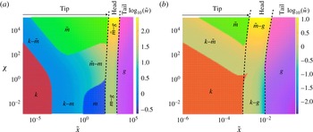
Numerical solution for the normalized fracture width $\tilde{w}$ (from the integral equation (3.11)) versus the spatial coordinate $\tilde{x}$ and the parameter ${\it\chi}$ for $\tilde{g}=10^{-9}$ (a) and $\tilde{g}=10^{6}$ (b). Red regions indicate areas of applicability of the toughness solution (4.1). The deep blue region in (a) indicates the area of applicability of the viscous solution (4.2). Green regions indicate areas of applicability of the leak-off solution (4.4). Magenta regions indicate areas of applicability of the tail solution (4.6). Dashed lines schematically indicate the tip region, the head region and the tail region.

To understand the structure of the solution, figure 2 shows the numerical solution of (3.11) and highlights the regions where the limiting solutions apply. Figure 2(a) shows the variation of the solution $\tilde{w}$ versus the spatial coordinate $\tilde{x}$ and the parameter ${\it\chi}$ for $\tilde{g}=10^{-9}$ , while figure 2(b) shows a similar solution map for $\tilde{g}=10^{6}$ . Red colouring indicates areas where the relative difference between the numerical solution and the toughness solution (4.1) is less than 1 %, and these areas are labelled with the ‘ $k$ ’ symbol. Similarly, blue colouring indicates the area where the viscous solution (4.2) is accurate to within 1 %, and this area is denoted by the ‘ $m$ ’ symbol. Green shading indicates regions where the leak-off solution (4.4) is accurate to within 1 %, and such areas are denoted by the ‘ $\tilde{m}$ ’ symbol. Finally, magenta highlights regions where the relative difference between the tail solution (4.6) and the numerical solution is below 1 %, and these regions are labelled with the ‘ $g$ ’ symbol. The toughness, viscous and leak-off asymptotic solutions appear in the tip region, then a transition region occurs which corresponds to the head, which is followed by the tail solution. There are regions where the solution evolves from one limiting solution to another, which are referred to as the ‘double transition regions’. Such transition regions will be analysed in § 5. There are also regions where three asymptotic solutions ‘meet’. Such cases are referred to as ‘triple transition regions’ and will be analysed in § 6. There is also a possibility when all four limiting solutions interplay simultaneously. This case is referred to as the ‘quadruple transition region’ and will be analysed in § 7. As was mentioned in the previous section, some parts of the analysis have been made previously. In particular, the analysis of the tip region is made in Garagash et al. (Reference Garagash, Detournay and Adachi2011), while Roper & Lister (Reference Roper and Lister2007) analysed the buoyancy-driven fracture for the large-toughness case. Despite this fact, this study aims to cover all transitions (i.e. those that were previously considered and the new ones) for completeness, and to perform the analysis by utilizing a non-singular equation formulation (3.11).

5 Double transitions

Section 4 outlined the limiting solutions and indicated their validity regions on the solution map (see figure 2). In addition, it highlighted the double transition regions, in which the transition from one limiting solution to another occurs. All such transition regions are schematically shown in figure 2, and are related to all possible combinations of two terms on the right-hand side of (3.15). This section focuses specifically on quantifying the solution in such transition regions. In order to do so, the scaling procedure for each transition is applied. The procedure to obtain this scaling is outlined below.

5.1 Scaling methodology

Let $i$ and $j$ correspond to two different limiting solutions, so that each of $i$ and $j$ corresponds to one of the quantities $\{k,m,\tilde{m},g\}$ , and $i\neq j$ . To obtain the scaling for the transition from the $i$ th to the $j$ th limiting solution, one should require

(5.1) $$\begin{eqnarray}\tilde{{\it\omega}}_{ij}\sim \tilde{w}_{i}(\tilde{l}_{ij})\sim \tilde{w}_{j}(\tilde{l}_{ij}),\end{eqnarray}$$

where $\tilde{w}_{i}$ and $\tilde{w}_{j}$ are selected from the solutions (4.1), (4.2), (4.4) or (4.5) based on the values of $i$ and $j$ , $\tilde{{\it\omega}}_{ij}$ is the scale for the fracture width for the ‘ $ij$ ’ transition, and $\tilde{l}_{ij}$ is the scale for the spatial coordinate; see Garagash et al. (Reference Garagash, Detournay and Adachi2011) where a similar approach is used. Here, ‘ ${\sim}$ ’ means equal up to a constant multiplier, so that all numerical multipliers can be omitted for simplicity. Justification for such a scaling procedure comes from (3.15), which indicates that if two terms on the right-hand side have similar magnitude, then both of them are important for the solution, and hence this corresponds to the transition. The scaling that comes from (5.1) can be summarized as

(5.2a,b ) $$\begin{eqnarray}\tilde{x}_{ij}={\displaystyle \frac{\tilde{x}}{\tilde{l}_{ij}}},\quad \tilde{w}_{ij}={\displaystyle \frac{\tilde{w}}{\tilde{{\it\omega}}_{ij}}},\end{eqnarray}$$

where $\tilde{x}_{ij}$ and $\tilde{w}_{ij}$ (note the difference between $\tilde{w}_{ij}$ and $\tilde{{\it\omega}}_{ij}$ ) are the scaled spatial coordinate and fracture width for the ‘ $ij$ ’ transition, and are both $O(1)$ . The latter statement should not be interpreted directly, since the integral equation features a multiplier $8/{\rm\pi}$ , which, combined with the fact that $G(t)=O(4)$ , implies that $32/{\rm\pi}=O(10)$ . The substitution ${\hat{s}}=(32/{\rm\pi})\tilde{s}$ (in this case $\tilde{g}$ also needs to be rescaled as ${\hat{g}}=({\rm\pi}/32)^{2}\tilde{g}$ ) would eliminate such numerical factors and would make the scaled quantities closer to $O(1)$ . Such a substitution would make the analysis more cumbersome, and therefore is not applied. It should be noted that the scaling (5.2) is a double scaling, i.e. a scaling that is performed in addition to (3.9). It should also be noted that scaled quantities that correspond to a particular transition regime are amended by a subscript with two letters, where the first letter represents the limiting regime from which the transition occurs and the second letter corresponds to the regime towards which the transition occurs (e.g. quantities that describe the transition from the toughness ( $k$ ) to the viscous ( $m$ ) regime are labelled with the ‘ $km$ ’ subscript). The next six subsections will consider all combinations of $i$ and $j$ from $\{k,m,\tilde{m},g\}$ ( $i\neq j$ ), and outline the governing equations and solutions for each of the transition regions.

5.2 Toughness–viscosity transition, $k{-}m$

To obtain the scaling for the $k{-}m$ transition, we let $i=k$ and $j=m$ in (5.1). In this case,

(5.3a-d ) $$\begin{eqnarray}\tilde{l}_{km}=1,\quad \tilde{{\it\omega}}_{km}=1,\quad \tilde{x}_{km}={\displaystyle \frac{\tilde{x}}{\tilde{l}_{km}}}=\tilde{x},\quad \tilde{w}_{km}={\displaystyle \frac{\tilde{w}}{\tilde{{\it\omega}}_{km}}}=\tilde{w}.\end{eqnarray}$$

The governing equation that describes this transition can be obtained from (3.11) by retaining only two relevant terms to yield

(5.4) $$\begin{eqnarray}\tilde{w}_{km}(\tilde{x}_{km})=1+{\displaystyle \frac{8}{{\rm\pi}}}\int _{0}^{\infty }G\left({\displaystyle \frac{\tilde{s}_{km}}{\tilde{x}_{km}}}\right){\displaystyle \frac{\text{d}\tilde{s}_{km}}{\tilde{w}_{km}(\tilde{s}_{km})^{2}}},\end{eqnarray}$$

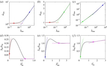
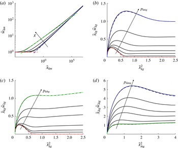
where the scaling (5.3) is applied. The numerical solution of (5.4) (solid black line) is shown in figure 3(a). Red and blue dashed lines indicate the toughness (4.1) and viscous (4.2) asymptotic solutions respectively. Red and blue circular markers show the locations at which asymptotic solutions become inaccurate. The level of accuracy is selected to be 1 %. Their values, calculated numerically, are

(5.5a,b ) $$\begin{eqnarray}\tilde{x}_{km}^{(1)}\approx 8.3\times 10^{-4},\quad \tilde{x}_{km}^{(2)}\approx 1.1,\end{eqnarray}$$

where the smaller value corresponds to the red marker (denoting the end of validity of the toughness solution), while the larger value corresponds to the blue marker (indicating the beginning of validity of the viscous solution).

Figure 3.

Scaled solutions in the transition regions (solid black lines): (a) toughness–viscous transition $k{-}m$ which is calculated from (5.4); (b) toughness–leak-off transition $k{-}\tilde{m}$ which is calculated from (5.7); (c) leak-off–viscous transition $\tilde{m}{-}m$ which is calculated from (5.10); (d) toughness–buoyancy transition $k{-}g$ which is calculated from (5.16); $(e)$ viscous–buoyancy transition $m{-}g$ which is calculated from (5.19);  $(f)$ leak-off–buoyancy transition $\tilde{m}{-}g$ which is calculated from (5.22). Red dashed lines indicate the toughness asymptotic solution (4.1). Blue dashed lines indicate the viscous asymptotic solution (4.2). Green dashed lines indicate the leak-off asymptotic solution (4.4). Magenta dashed lines show the tail solution (4.6). Coloured circular markers indicate locations at which the accuracy of the corresponding asymptotic solutions is below 1 %.

5.3 Toughness–solidification (leak-off) transition, $k{-}\tilde{m}$

Similarly, the transition from the toughness to the leak-off regime requires $i=k$ and $j=\tilde{m}$ , in which case the length scale and normalized width are

(5.6a-d ) $$\begin{eqnarray}\tilde{l}_{k\tilde{m}}={\displaystyle \frac{1}{{\it\chi}}},\quad \tilde{{\it\omega}}_{k\tilde{m}}=1,\quad \tilde{x}_{k\tilde{m}}={\displaystyle \frac{\tilde{x}}{\tilde{l}_{k\tilde{m}}}}={\it\chi}\tilde{x},\quad \tilde{w}_{k\tilde{m}}={\displaystyle \frac{\tilde{w}}{\tilde{{\it\omega}}_{k\tilde{m}}}}=\tilde{w}.\end{eqnarray}$$

The equation that governs this transition is

(5.7) $$\begin{eqnarray}\tilde{w}_{k\tilde{m}}(\tilde{x}_{k\tilde{m}})=1+{\displaystyle \frac{8}{{\rm\pi}}}\int _{0}^{\infty }G\left({\displaystyle \frac{\tilde{s}_{k\tilde{m}}}{\tilde{x}_{k\tilde{m}}}}\right){\displaystyle \frac{\text{d}\tilde{s}_{k\tilde{m}}}{\tilde{w}_{k\tilde{m}}(\tilde{s}_{k\tilde{m}})^{3}}},\end{eqnarray}$$

where the result is obtained from (3.11) by retaining only the ‘toughness’ and ‘leak-off’ terms and using the scaling (5.6). The numerical solution of (5.7) (solid black line) is shown in figure 3(b). Red and green dashed lines indicate the toughness (4.1) and leak-off (4.4) asymptotic solutions respectively. The red and green circular markers show locations at which the accuracy of the asymptotic solutions becomes less than 1 %. These locations are calculated numerically, and are given by

(5.8a,b ) $$\begin{eqnarray}\tilde{x}_{k\tilde{m}}^{(1)}\approx 8.3\times 10^{-4},\quad \tilde{x}_{k\tilde{m}}^{(2)}\approx 0.6,\end{eqnarray}$$

where the smaller value corresponds to the red marker (end of validity of the toughness solution), while the larger value corresponds to the green marker (beginning of validity of the leak-off solution).

5.4 Solidification (leak-off)–viscosity transition, $\tilde{m}{-}m$

To describe the transition from the leak-off to the viscosity regime, let $i=\tilde{m}$ and $j=m$ in (5.1). The corresponding scalings for the spatial coordinate and the width are

(5.9a-d ) $$\begin{eqnarray}\tilde{l}_{\tilde{m}m}={\it\chi}^{3},\quad \tilde{{\it\omega}}_{\tilde{m}m}={\it\chi},\quad \tilde{x}_{\tilde{m}m}={\displaystyle \frac{\tilde{x}}{\tilde{l}_{\tilde{m}m}}}={\it\chi}^{-3}\tilde{x},\quad \tilde{w}_{\tilde{m}m}={\displaystyle \frac{\tilde{w}}{\tilde{{\it\omega}}_{\tilde{m}m}}}={\it\chi}^{-1}\tilde{w},\end{eqnarray}$$

while the scaled governing equation is obtained by retaining only the viscosity-related and leak-off-related terms in (3.11), and applying the scaling (5.9) to yield

(5.10) $$\begin{eqnarray}\tilde{w}_{\tilde{m}m}(\tilde{x}_{\tilde{m}m})={\displaystyle \frac{8}{{\rm\pi}}}\int _{0}^{\infty }G\left({\displaystyle \frac{\tilde{s}_{\tilde{m}m}}{\tilde{x}_{\tilde{m}m}}}\right)\left[{\displaystyle \frac{1}{\tilde{w}_{\tilde{m}m}(\tilde{s}_{k\tilde{m}})^{2}}}+{\displaystyle \frac{1}{\tilde{w}_{\tilde{m}m}(\tilde{s}_{k\tilde{m}})^{3}}}\right]\,\text{d}\tilde{s}_{\tilde{m}m}.\end{eqnarray}$$

Figure 3(c) shows the numerical solution of (5.10) (solid black line), and indicates the leak-off (4.4) and viscous (4.2) asymptotic solutions by green and blue dashed lines respectively. Green and blue circular markers show locations at which the accuracy of the above asymptotic solutions becomes less than 1 %, and are calculated as

(5.11a,b ) $$\begin{eqnarray}\tilde{x}_{\tilde{m}m}^{(1)}\approx 1.5\times 10^{-7},\quad \tilde{x}_{\tilde{m}m}^{(2)}\approx 3.8\times 10^{3},\end{eqnarray}$$

where the smaller value corresponds to the green marker (end of validity of the leak-off solution), while the larger value corresponds to the blue marker (beginning of validity of the viscous solution).

The numerical solutions shown in figure 3(a–c) correspond to the transitions in the absence of (or negligible) buoyancy. Such transitions are consistent with the findings in Garagash et al. (Reference Garagash, Detournay and Adachi2011) and are added for completeness. It should also be noted that a closed-form approximate solution that captures the solution in the absence of buoyancy (which, in particular, captures all three transition regions described above) is obtained in Dontsov & Peirce (Reference Dontsov and Peirce2015). In order to understand the influence of buoyancy, it is necessary to add three additional transition regions, in which transition from one of the limiting tip solutions (toughness, viscous or leak-off) to the tail occurs.

5.5 Toughness–buoyancy transition, $k{-}g$

In the situation where the transition from the tip to the head (and further to the tail) occurs in the toughness regime, $i=\tilde{k}$ and $j=g$ in (5.1). In this case, the associated scaling for the transition is

(5.12a-d ) $$\begin{eqnarray}\tilde{l}_{kg}={\displaystyle \frac{1}{\tilde{g}^{1/3}}},\quad \tilde{{\it\omega}}_{kg}=1,\quad \tilde{x}_{kg}={\displaystyle \frac{\tilde{x}}{\tilde{l}_{kg}}}=\tilde{g}^{1/3}\tilde{x},\quad \tilde{w}_{kg}={\displaystyle \frac{\tilde{w}}{\tilde{{\it\omega}}_{kg}}}=\tilde{w}.\end{eqnarray}$$

The governing equation for this transition in the scaling (5.12) can be formulated as

(5.13) $$\begin{eqnarray}\tilde{w}_{kg}(\tilde{x})=1+{\displaystyle \frac{8}{{\rm\pi}}}\int _{0}^{\infty }G\left({\displaystyle \frac{\tilde{s}_{kg}}{\tilde{x}_{kg}}}\right)f(\tilde{s}_{kg})\,\text{d}\tilde{s}_{kg},\end{eqnarray}$$

where two relevant terms are considered, namely the ‘toughness’ term and the ‘gravity’ term. The difficulty comes from the fact that the solution has two regions, the head ( $\tilde{x}_{kg}<\tilde{x}_{0}$ ) and the tail ( $\tilde{x}_{kg}>\tilde{x}_{0}$ ), where $\tilde{x}_{0}$ is the unknown head length. The fracture width in the head is unknown, but is zero in the tail, i.e.

(5.14) $$\begin{eqnarray}\tilde{w}(\tilde{x}_{kg})\equiv 0,\quad \tilde{x}_{kg}>\tilde{x}_{0}.\end{eqnarray}$$

At the same time, the buoyancy term is known in the head region,

(5.15a,b ) $$\begin{eqnarray}f(\tilde{s}_{kg})=-\tilde{s}_{kg}^{2},\quad \tilde{x}_{kg}<\tilde{x}_{0},\end{eqnarray}$$

while its contribution from the tail is unknown (since the buoyancy term competes with the viscous term, which for zero viscosity and zero fracture width can produce non-trivial contributions). This formulation makes it difficult to tackle the problem. This problem, however, has been solved in Roper & Lister (Reference Roper and Lister2007) using a different approach, and the solution for the head, written in the scaling (5.12), is

(5.16a,b ) $$\begin{eqnarray}\tilde{w}_{kg}=(1-2^{2/3}\tilde{x}_{kg}^{2})^{3/2},\quad \tilde{x}_{kg}<\tilde{x}_{0}=2^{-1/3}.\end{eqnarray}$$

Figure 3(d) plots the solution (5.16) (solid black line) in terms of $\tilde{x}_{kg}\tilde{w}_{kg}$ (which is a fracture width that is normalized by the constants only, and not by a spatial coordinate) and $\tilde{x}_{kg}^{2}$ (which is the normalized physical distance from the fracture tip). The toughness asymptotic solution (4.1) is indicated by the red dashed line, while the tail solution (which is zero in this case) is shown by the magenta dashed line. Red and magenta circular markers denote locations at which the accuracy of the asymptotic solutions becomes less than 1 %, and are calculated as

(5.17a,b ) $$\begin{eqnarray}\tilde{x}_{kg}^{(1)}\approx 6.5\times 10^{-2},\quad \tilde{x}_{kg}^{(2)}\approx 0.8.\end{eqnarray}$$

Here, the smaller value corresponds to the red marker (end of validity of the toughness solution), while the larger value corresponds to the magenta marker (beginning of validity of the tail solution).

5.6 Viscosity–buoyancy transition, $m{-}g$

To describe the transition from the viscosity-dominated tip to the head, let $i=m$ and $j=g$ in (5.1). In this case, the scaling is

(5.18a-d ) $$\begin{eqnarray}\tilde{l}_{mg}={\displaystyle \frac{1}{\tilde{g}^{3/8}}},\quad \tilde{{\it\omega}}_{mg}={\displaystyle \frac{1}{\tilde{g}^{1/8}}},\quad \tilde{x}_{mg}={\displaystyle \frac{\tilde{x}}{\tilde{l}_{mg}}}=\tilde{g}^{3/8}\tilde{x},\quad \tilde{w}_{mg}={\displaystyle \frac{\tilde{w}}{\tilde{{\it\omega}}_{mg}}}=\tilde{g}^{1/8}\tilde{w}.\end{eqnarray}$$

By retaining only the viscous and buoyancy terms in (3.11), and applying the scaling (5.18), one has

(5.19) $$\begin{eqnarray}\tilde{w}_{mg}(\tilde{x})={\displaystyle \frac{8}{{\rm\pi}}}\int _{0}^{\infty }G\left({\displaystyle \frac{\tilde{s}_{mg}}{\tilde{x}_{mg}}}\right)\left[{\displaystyle \frac{1}{\tilde{w}_{mg}(\tilde{s}_{mg})^{2}}}-\tilde{s}_{mg}^{2}\right]\,\text{d}\tilde{s}_{mg}.\end{eqnarray}$$

Figure 3(e) plots the solution (5.19) (solid black line) in terms of $\tilde{x}_{mg}\tilde{w}_{mg}$ and $\tilde{x}_{mg}^{2}$ , similarly to the previous case. The viscous asymptotic solution (4.2) is shown by the blue dashed line, while the tail solution (4.6) (which is equal to unity in the adopted scaling) is shown by the magenta dashed line. Blue and magenta circular markers show locations at which the accuracy of the asymptotic solutions becomes less than 1 %, and are calculated as

(5.20a,b ) $$\begin{eqnarray}\tilde{x}_{mg}^{(1)}\approx 9\times 10^{-2},\quad \tilde{x}_{mg}^{(2)}\approx 1.4,\end{eqnarray}$$

where the smaller value corresponds to the blue marker (end of validity of the viscous solution), while the larger value corresponds to the magenta marker (beginning of validity of the tail solution). It is interesting to note that the solution features a ‘neck’, which occurs after the magenta marker and where the fracture width is smaller than the tail solution. This feature, however, does not have a substantial magnitude for the transition regime considered.

5.7 Solidification (leak-off)–buoyancy transition, $\tilde{m}{-}g$

The last transition to consider is the transition from the leak-off (solidification) dominance to buoyancy, in which case $i=\tilde{m}$ and $j=g$ . The scaling can be calculated from (5.1) as

(5.21a-d ) $$\begin{eqnarray}\tilde{l}_{\tilde{m}g}={\displaystyle \frac{{\it\chi}^{1/11}}{\tilde{g}^{4/11}}},\quad \tilde{{\it\omega}}_{\tilde{m}g}={\displaystyle \frac{{\it\chi}^{3/11}}{\tilde{g}^{1/11}}},\quad \tilde{x}_{\tilde{m}g}={\displaystyle \frac{\tilde{x}}{\tilde{l}_{\tilde{m}g}}}={\displaystyle \frac{\tilde{g}^{4/11}}{{\it\chi}^{1/11}}}\tilde{x},\quad \tilde{w}_{\tilde{m}g}={\displaystyle \frac{\tilde{w}}{\tilde{{\it\omega}}_{\tilde{m}g}}}={\displaystyle \frac{\tilde{g}^{1/11}}{{\it\chi}^{3/11}}}\tilde{w}.\end{eqnarray}$$

By retaining only the leak-off and buoyancy terms in (3.11), and using the scaling (5.21), one obtains

(5.22) $$\begin{eqnarray}\tilde{w}_{\tilde{m}g}(\tilde{x})={\displaystyle \frac{8}{{\rm\pi}}}\int _{0}^{\infty }G\left({\displaystyle \frac{\tilde{s}_{\tilde{m}g}}{\tilde{x}_{\tilde{m}g}}}\right)\left[{\displaystyle \frac{1}{\tilde{w}_{\tilde{m}g}(\tilde{s}_{\tilde{m}g})^{3}}}-\tilde{s}_{\tilde{m}g}^{2}\right]\,\text{d}\tilde{s}_{\tilde{m}g}.\end{eqnarray}$$

Figure 3(f) plots the solution (5.22) (solid black line) in terms of $\tilde{x}_{\tilde{m}g}\tilde{w}_{\tilde{m}g}$ and $\tilde{x}_{\tilde{m}g}^{2}$ . The leak-off asymptotic solution (4.4) is represented by the green dashed line, while the tail solution (4.6) (which is equal to $\tilde{x}_{\tilde{m}g}^{-2/3}$ for this case) is indicated by the magenta dashed line. Green and magenta circular markers indicate locations at which the accuracy of the asymptotic solutions becomes less than 1 %. Their locations are calculated as

(5.23a,b ) $$\begin{eqnarray}\tilde{x}_{\tilde{m}g}^{(1)}\approx 0.1,\quad \tilde{x}_{\tilde{m}g}^{(2)}\approx 1.2,\end{eqnarray}$$

where the smaller value corresponds to the green marker (end of validity of the leak-off solution), while the larger value corresponds to the magenta marker (beginning of validity of the tail solution). The solution also features a local maximum followed by a local minimum in the ‘neck’ region, both of which have relatively insignificant prominence.

Figure 4.

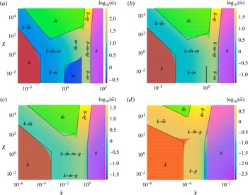
Numerical solution for the normalized fracture width $\tilde{w}$ (from the integral equation (3.11)) versus the spatial coordinate $\tilde{x}$ and the parameter ${\it\chi}$ for $\tilde{g}=10^{-9}$ (a), $\tilde{g}=10^{-3}$ (b), $\tilde{g}=1$ (c) and $\tilde{g}=10^{9}$ (d). Red regions indicate areas of applicability of the toughness solution (4.1). The deep blue region in (a) indicates the area of applicability of the viscous solution (4.2). Green regions indicate areas of applicability of the leak-off solution (4.4). Magenta regions indicate areas of applicability of the tail solution (4.6). Solid black lines indicate the boundaries of applicability of the transition solutions that are given in (5.5), (5.8), (5.11), (5.17), (5.20) and (5.23).

6 Triple transitions

This section focuses on triple transitions, which are the regions in which three out of the four terms on the right-hand side of (3.15) are commensurate in magnitude, while the fourth term can be neglected. There are four such transition regions, and they are described next.

Figure 5.

Numerical solutions for triple transitions (solid black lines): (a) toughness–solidification (leak-off)–viscosity transition $k{-}\tilde{m}{-}m$ , solution of (6.1) for ${\it\chi}=\{0.1,1,10,10^{2}\}$ ; (b) toughness–viscosity–buoyancy transition $k{-}m{-}g$ , solution of (6.3) for $\log _{10}(p_{kmg})=\{-3,-2,-1.5,-1,-0.5,0\}$ ; (c) toughness–solidification (leak-off)–buoyancy transition $k{-}\tilde{m}{-}g$ , solution of (6.4) for $\log _{10}(p_{kmg})=\{-4,-3,-2,-1,-0.5,0\}$ ; (d) solidification (leak-off)–viscosity–buoyancy transition $\tilde{m}{-}m{-}g$ , solution of (6.6) for $\log _{10}(p_{\tilde{m}mg})=\{-1,0,0.5,0.75,1,1.25\}$ . The dashed red, blue and green lines in (a) correspond to the limiting solutions (4.1), (4.2) and (4.4). The dashed red, blue and green lines in (b–d) correspond to the double transition solutions $k{-}g$ , $k{-}m$ and $\tilde{m}{-}m$ which are shown in figure 3(d–f).

6.1 Toughness–solidification (leak-off)–viscosity transition, $k{-}\tilde{m}{-}m$

To concentrate on the $k{-}\tilde{m}{-}m$ transition, one should disregard the buoyancy term in (3.11), which yields

(6.1) $$\begin{eqnarray}\tilde{w}_{km}(\tilde{x})=1+{\displaystyle \frac{8}{{\rm\pi}}}\int _{0}^{\infty }G\left({\displaystyle \frac{\tilde{s}_{km}}{\tilde{x}_{km}}}\right)\left[{\displaystyle \frac{1}{\tilde{w}_{km}(\tilde{s}_{km})^{2}}}+{\displaystyle \frac{{\it\chi}}{\tilde{w}_{km}(\tilde{s}_{km})^{3}}}\right]\,\text{d}\tilde{s}_{km},\end{eqnarray}$$

where the result is written in the ‘ $km$ ’ scaling (5.3). It should be noted that this regime describes the transition that occurs solely at the fracture tip. Practically, this regime appears when $\tilde{x}_{mg}^{(1)}\tilde{l}_{mg}\gg \tilde{x}_{km}^{(2)}\tilde{l}_{km}$ , in which case there is a well-established viscous zone. By taking the values of $\tilde{x}_{mg}^{(1)}$ from (5.20) and $\tilde{x}_{km}^{(2)}$ from (5.5), and the length scales from (5.3) and (5.18), we can conclude that such a transition can occur for

(6.2) $$\begin{eqnarray}\tilde{g}\ll 1.3\times 10^{-3},\end{eqnarray}$$

which is consistent with the result shown in figure 4. The latter figure shows that the viscous zone starts to appear for $\tilde{g}=10^{-3}$ . The dimensionless parameter that influences the solution of (6.1) is ${\it\chi}$ . To understand the influence of the parameter ${\it\chi}$ , figure 5(a) plots the numerical solution of (6.1) for ${\it\chi}=\{0.1,1,10,10^{2}\}$ . The arrow indicates the direction in which the solutions move as ${\it\chi}$ increases. The red, blue and green dashed lines indicate the limiting solutions (4.1), (4.2) and (4.4) respectively. It should be noted that the leak-off solution (4.4) is plotted only for the largest value of ${\it\chi}=10^{2}$ . It is clear that for small values of ${\it\chi}$ the solution reduces to the $k{-}m$ transition (5.4) (see figure 3 a). For large values of ${\it\chi}$ , the $k{-}\tilde{m}$ transition (5.7) (see figure 3 b) appears first, which is followed by the $\tilde{m}-m$ transition (5.10) (see figure 3 c). This demonstrates that the limiting behaviour of the considered triple transition is captured by double transitions that are described in the previous section.

6.2 Toughness–viscosity–buoyancy transition, $k{-}m{-}g$

The $k{-}m{-}g$ transition occurs when the leak-off term in (3.11) is negligible, i.e. ${\it\chi}\ll 1$ . The governing integral equation, written in terms of the ‘ $kg$ ’ scaling (5.12), is

(6.3) $$\begin{eqnarray}\tilde{w}_{kg}(\tilde{x}_{kg})=1+{\displaystyle \frac{8}{{\rm\pi}}}\int _{0}^{\infty }G\left({\displaystyle \frac{\tilde{s}_{kg}}{\tilde{x}_{kg}}}\right)\left[{\displaystyle \frac{p_{kmg}}{\tilde{w}_{kg}(\tilde{s}_{kg})^{2}}}-\tilde{s}_{kg}^{2}\right]\,\text{d}\tilde{s}_{kg},\end{eqnarray}$$

where $p_{kmg}=\tilde{g}^{-1/3}$ is a parameter. Figure 5(b) plots the numerical solution of (6.3) for $\log _{10}(p_{kmg})=\{-3,-2,-1.5,-1,-0.5,0\}$ . The arrow indicates the direction in which the solution changes as the parameter $p_{kmg}$ increases. The red dashed line shows the $k{-}g$ solution (5.16) (see figure 3 d). The blue dashed line shows the $m{-}g$ solution (5.19) (see figure 3 e). It should be noted that the $m{-}g$ solution is plotted only for the largest value of the parameter $p_{kmg}=1$ . For small values of the parameter $p_{kmg}$ , the solution follows the $k{-}g$ solution, and gradually transitions to the $m{-}g$ solution as the parameter $p_{kmg}$ increases. It should be noted that the toughness-to-viscous $k{-}m$ transition occurs at the tip.

6.3 Toughness–solidification (leak-off)–buoyancy transition, $k{-}\tilde{m}{-}g$

The $k{-}\tilde{m}{-}g$ transition occurs when the effect of viscosity can be neglected in (3.11). The corresponding governing integral equation, written in the ‘ $kg$ ’ scaling (5.12), is

(6.4) $$\begin{eqnarray}\tilde{w}_{kg}(\tilde{x}_{kg})=1+{\displaystyle \frac{8}{{\rm\pi}}}\int _{0}^{\infty }G\left({\displaystyle \frac{\tilde{s}_{kg}}{\tilde{x}_{kg}}}\right)\left[{\displaystyle \frac{p_{k\tilde{m}g}}{\tilde{w}_{kg}(\tilde{s}_{kg})^{3}}}-\tilde{s}_{kg}^{2}\right]\,\text{d}\tilde{s}_{kg},\end{eqnarray}$$

where the parameter is $p_{k\tilde{m}g}={\it\chi}\tilde{g}^{-1/3}$ . As follows from figure 4, the triple transition under consideration occurs in the situation when the viscous zone and the associated transition zones disappear. In order for this situation to occur, one should require $\tilde{x}_{km}^{(1)}\tilde{l}_{km}\gg \tilde{x}_{kg}^{(1)}\tilde{l}_{kg}$ , which with the use of (5.3), (5.12), (5.5) and (5.17) implies that

(6.5) $$\begin{eqnarray}\tilde{g}\gg 5\times 10^{5}.\end{eqnarray}$$

Figure 5(c) plots the numerical solution of (6.4) for $\log _{10}(p_{kmg})=\{-4,-3,-2,-1,-0.5,0\}$ . The arrow indicates the direction in which the solution changes as the parameter $p_{k\tilde{m}g}$ increases. The red dashed line shows the $k{-}g$ solution (5.16) (see figure 3 d). The green dashed line shows the $\tilde{m}{-}g$ solution (5.22) (see figure 3 f). It should be noted that the $\tilde{m}{-}g$ solution is plotted only for the largest value of the parameter $p_{k\tilde{m}g}=1$ . For small values of the parameter $p_{k\tilde{m}g}$ , the solution follows the $k{-}g$ solution, and gradually transitions to the $\tilde{m}{-}g$ solution as the parameter $p_{k\tilde{m}g}$ increases. It should be noted that the toughness-to-leak-off $k{-}\tilde{m}$ transition occurs at the tip.

Figure 6.

Schematics of the $({\it\chi},\tilde{g})$ map of the solution, obtained based on the limiting values of the parameters $p_{pmg}$ , $p_{k\tilde{m}g}$ and $p_{\tilde{m}mg}$ featured in (6.3), (6.4) and (6.6).

6.4 Solidification (leak-off)–viscosity–buoyancy transition, $\tilde{m}{-}m{-}g$

The $\tilde{m}{-}m{-}g$ transition occurs when the effect of fracture toughness is negligible in (3.11). In this situation, it is convenient to adopt the ‘ $\tilde{m}g$ ’ scaling (5.21), disregard the toughness-related term, and rewrite (3.11) as

(6.6) $$\begin{eqnarray}\tilde{w}_{\tilde{m}g}(\tilde{x}_{\tilde{m}g})={\displaystyle \frac{8}{{\rm\pi}}}\int _{0}^{\infty }G\left({\displaystyle \frac{\tilde{s}_{\tilde{m}g}}{\tilde{x}_{\tilde{m}g}}}\right)\left[{\displaystyle \frac{p_{\tilde{m}mg}}{\tilde{w}_{\tilde{m}g}(\tilde{s}_{\tilde{m}g})^{2}}}+{\displaystyle \frac{1}{\tilde{w}_{\tilde{m}g}(\tilde{s}_{\tilde{m}g})^{3}}}-\tilde{s}_{\tilde{m}g}^{2}\right]\,\text{d}\tilde{s}_{\tilde{m}g},\end{eqnarray}$$

where the parameter is $p_{\tilde{m}mg}={\it\chi}^{-8/11}\tilde{g}^{-1/11}$ . This transition may occur only if a viscous zone exists, i.e. when $\tilde{g}\ll 1.3\times 10^{-3}$ ; see (6.2). To quantify the transition, figure 5(d) plots the numerical solution of (6.6) for $\log _{10}(p_{\tilde{m}mg})=\{-1,0,0.5,0.75,1,1.25\}$ . As for the previous plots, the arrow indicates the direction in which the solution changes as the parameter $p_{\tilde{m}mg}$ increases. The green dashed line shows the $\tilde{m}{-}g$ solution (5.22) (see figure 3 f). The blue dashed line shows the $m{-}g$ solution (5.19) (see figure 3 e). It should be noted that the $m{-}g$ solution is plotted only for the largest value of the parameter $p_{k\tilde{m}g}=10^{1.25}\approx 18$ . For small values of the parameter $p_{\tilde{m}mg}$ , the solution is close to the $\tilde{m}{-}g$ solution, and gradually transitions to the $m{-}g$ solution as the parameter $p_{\tilde{m}mg}$ increases. It should be noted that the leak-off-to-viscous $\tilde{m}{-}m$ transition occurs at the tip.

Figure 7.

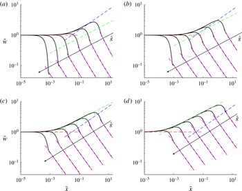
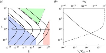
Solutions of the integral equation (3.11) in terms of scaled variables (3.9) for different values of the solidification parameter ${\it\chi}=\{10^{-1},1,10,10^{2}\}$ and buoyancy parameter $\tilde{g}=\{10^{-1},10^{1},10^{3},10^{5},10^{7},10^{9}\}$ (solid black lines). Arrows schematically indicate the direction in which solutions shift for increasing values of the buoyancy parameter $\tilde{g}$ , so that the ‘rightmost’ solutions correspond to $\tilde{g}=10^{-1}$ , while the ‘leftmost’ solutions correspond to $\tilde{g}=10^{9}$ . Dashed red lines represent the toughness asymptotic solution (4.1), dashed blue lines correspond to the viscous asymptotic solution (4.2), dashed green lines correspond to the leak-off asymptotic solution (4.4), while dashed magenta lines show the tail solution (4.6).

6.5 The $({\it\chi},\tilde{g})$ map of the solution

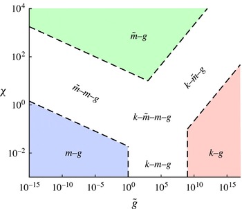
The results of this section are summarized in figure 6, which shows the schematics of the solution map in the $({\it\chi},\tilde{g})$ plane. The dashed black lines depict the limiting values of the parameters $p_{pmg}$ , $p_{k\tilde{m}g}$ and $p_{\tilde{m}mg}$ , featured in (6.3), (6.4) and (6.6) respectively. It should be noted that this is a schematic, and the limiting values of $p_{pmg}$ , $p_{k\tilde{m}g}$ and $p_{\tilde{m}mg}$ are chosen as a measure to separate the regions. Red, blue and green regions indicate zones in which the $k{-}g$ , $m{-}g$ and $\tilde{m}{-}g$ solutions apply respectively. It should also be noted that the $k{-}m{-}g$ transition occurs for $1<\tilde{g}<10^{9}$ , which is not in agreement with (6.2) and (6.5). The latter two equations actually estimate the applicability of the tip asymptote, while the current map estimates the applicability of the whole solution in the head region. It can happen that the tip asymptote is in the toughness zone, but the whole solution is not in good agreement with the $k{-}g$ solution due to large discrepancies at the beginning of the tail region. It is also important to emphasize that the map shown in figure 6 is based on the comparison of the solution in the head region (and the beginning of the tail region). The tail regions for the $m{-}g$ and $k{-}g$ solutions will disagree with a solution with finite ${\it\chi}$ at some distance even for very small values of ${\it\chi}$ . This happens since the solution is constant in the tail region for the $m{-}g$ and $k{-}g$ solutions, while it grows with distance as soon as ${\it\chi}>0$ is introduced. This feature makes quantitative estimation of the solution zones somewhat problematic.

Figure 8.

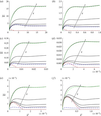
Solutions (solid black lines) of the integral equation (3.11) in terms of scaled variables (3.9) for different values of the solidification parameter ${\it\chi}=\{10^{-1},1,10,10^{2}\}$ and with buoyancy parameter $\tilde{g}$ equal to (a) $10^{-1}$ , (b) $10^{1}$ , (c) $10^{3}$ , (d) $10^{5}$ , (e) $10^{7}$ and (f) $10^{9}$ . Arrows schematically indicate the direction in which solutions shift for increasing values of the leak-off parameter ${\it\chi}$ , so that the ‘lowermost’ solutions correspond to ${\it\chi}=10^{-1}$ , while the ‘uppermost’ solutions correspond to ${\it\chi}=10^{2}$ . Dashed red, blue and green lines indicate the double transition solutions $k{-}g$ , $m{-}g$ and  $\tilde{m}{-}g$ respectively, as in figure 3(d–f). It should be noted that the $\tilde{m}{-}g$ solutions (dashed green lines) are plotted only for ${\it\chi}=10^{2}$ , while the solutions $k{-}g$ and $m{-}g$ are independent of ${\it\chi}$ . The ordinate $\tilde{x}\tilde{w}$ is the normalized fracture width, which is scaled by spatially constant quantities, while the abscissa $\tilde{x}^{2}$ is the normalized spatial coordinate; see the scaling (3.9).

7 Quadruple transition

In order to quantify the solution in the situation when all four terms in the governing integral equation (3.11) are relevant, figures 7 and 8 plot the numerical solution for the following parameter set: ${\it\chi}=\{10^{-1},1,10,10^{2}\}$ and $\tilde{g}=\{10^{-1},10^{1},10^{3},10^{5},10^{7},10^{9}\}$ . Figure 7 shows the solutions on a logarithmic scale, which enables us to analyse the multiscale behaviour of the tip region. At the same time, figure 8 shows the same solutions, but on a linear scale, which allows us to analyse the shape of the fracture head zone. It should also be noted that $\tilde{x}\tilde{w}$ is the normalized fracture width, which is scaled by spatially constant quantities (as opposed to $\tilde{w}$ , which is scaled by the spatial coordinate). The abscissa $\tilde{x}^{2}$ is the normalized spatial coordinate (as opposed to $\tilde{x}$ , which is proportional to the square root of the spatial coordinate); see the scaling (3.9).

Figure 7 also shows the limiting solutions that correspond to the toughness solution (4.1) (dashed red lines), viscous solution (4.2) (dashed blue lines), leak-off solution (4.4) (dashed green lines) and tail solution (4.6) (dashed magenta lines). One can observe an interplay between different asymptotic solutions at the fracture tip, in which either one of them dominates, two of them dominate or all three affect the fracture tip behaviour. The parameters for which all three asymptotic tip solutions are close, and therefore have a strong influence on the tip behaviour, is truly the quadruple transition.

The primary advantage of the data representation in figure 8 lies in the fact that one can clearly observe the fracture head shape and compare it with one of the double transition solutions. For the purpose of comparison with the double transition solutions, dashed red, blue and green lines in figure 8 show the $k{-}g$ , $m{-}g$ and $\tilde{m}{-}g$ double transition solutions respectively, as in figure 3(d–f). It should be noted that the $\tilde{m}{-}g$ solutions (dashed green lines) are plotted only for ${\it\chi}=10^{2}$ , while the solutions $k{-}g$ and $m{-}g$ are independent of ${\it\chi}$ . For the $\tilde{g}=10^{-1}$ case, the solutions clearly transition from the $m{-}g$ to the $\tilde{m}{-}g$ solution, which is similar to what is shown in figure 5(d). One should note the different scaling used for plotting figure 5(d), in which case the transition looks reversed. For the largest $\tilde{g}=10^{9}$ considered, the solution transitions from the $k{-}g$ (i.e. red dashed line) to the $\tilde{m}{-}g$ (i.e. dashed green line) solution, which is similar to what is shown in figure 5(c). Other values of $\tilde{g}$ represent intermediate cases, in which the solution for the smallest solidification parameter ${\it\chi}=10^{-1}$ corresponds to the $k{-}m{-}g$ triple transition; see figure 5(b). Solutions for all $\tilde{g}$ eventually reach the $\tilde{m}{-}g$ regime for large values of ${\it\chi}$ . It is important to note that the parameter ${\it\chi}$ is able to accurately describe the transition to the $\tilde{m}{-}g$ regime for the intermediate values of $\tilde{g}$ (in the sense that the solution reaches its limiting behaviour for large values of ${\it\chi}$ ). This is not the case for small and very large values of $\tilde{g}$ . The reason for this lies in the fact that the $k{-}\tilde{m}{-}g$ transition (which is, practically, what happens for $\tilde{g}=10^{9}$ ) is determined by the parameter $p_{k\tilde{m}g}={\it\chi}\tilde{g}^{-1/3}$ , as shown in the previous section. In this situation, $p_{k\tilde{m}g}\gg 1$ leads to the $\tilde{m}{-}g$ limit, and the criterion ${\it\chi}\gg 1$ is not sufficient (considering a broad variation of $\tilde{g}$ ). This is consistent with the results shown in figure 6, which indicates that values of ${\it\chi}$ larger than $10^{2}$ are required to transition to the $\tilde{m}{-}g$ solution in situations when $\tilde{g}\gtrsim 10^{7}$ . Likewise, the $\tilde{m}{-}m{-}g$ transition practically occurs for $\tilde{g}=10^{-1}$ . As follows from (6.6), the parameter that describes the transition from the $m{-}g$ to the $\tilde{m}{-}g$ solution is $p_{\tilde{m}mg}={\it\chi}^{-8/11}\tilde{g}^{-1/11}$ . Since this parameter depends on $\tilde{g}$ , the criterion ${\it\chi}\gg 1$ is not a universal criterion for all values of $\tilde{g}$ .

It is also interesting to mention that the solutions shown in figure 8 depict the normalized width of the channel in which the magma flows. This is different from the total width, which also accounts for the width of the solidified magma layer (3.13). In order to estimate the effect of the solidified layer, one should focus on figure 7, noting that $\tilde{w}_{s}\approx {\it\chi}=\text{const}$ . It is clear that since $\tilde{w}(\tilde{x})\rightarrow 0$ in the tail region, the width of the solidified layer becomes much larger than the width of the flowing magma away from the fracture head (even for small values of ${\it\chi}$ ). For the cases ${\it\chi}=10$ and ${\it\chi}=100$ , $\tilde{w}_{s}>\tilde{w}$ for all $\tilde{x}$ , which includes the head region. In these situations, the total width can be approximated reasonably accurately by $\tilde{w}_{s}$ . The dynamics of the fracture, however, is still related to the solution $\tilde{w}$ .

8 Possible applications of the results

The developed analysis and solution can be used in multiple ways. First, it can be used to test non-steady calculations. In particular, it can test whether the procedure for calculating non-steady propagation captures all limiting regimes and transitions between them. Second, the steady solution can be applied to analyse buoyancy-driven hydraulic fracture propagation in situations when the fracture propagation velocity changes slowly, in which case the steady solution applies. Section 9 gives an example to illustrate this application. Finally, the results demonstrate the presence of distinct regimes of propagation and characterize differences in the head and tail shapes. This can be used to interpret laboratory results. For instance, if the fracture aperture in the head region is substantially larger than in the tail, then fracture toughness plays the dominant role; see e.g. the dashed red line in figure 8. If the fracture width in the tail is constant and is comparable to the head region, then the response is dominated by the fluid viscosity (so that fracture toughness does not noticeably influence the solution); see e.g. the dashed blue line in figure 8. Finally, the results of this paper can be used to compare the regimes of propagation for laboratory experiment parameters and for field data. This can help to improve the design of the experimental set-up, ensuring proper scaling and correspondence between laboratory-size experiments and field observations.

9 Application to a non-steady fracture

Let us now consider a finite buoyancy-driven hydraulic fracture, which is fed by a source with constant intensity $Q_{0}$ ( $\text{m}^{2}~\text{s}^{-1}$ ), as shown in figure 1. The fracture length, $l$ , is measured from the source, while $V$ is the velocity of fracture propagation. To simplify the problem, the solution is approximated by the steady solution for which the propagation velocity varies slowly. In addition, it is implicitly assumed that the size of the fracture head is much smaller than the length of the fracture, in which case the effect of the free surface near the source can be neglected. This corresponds to the solution at large time.

In order to be able to provide a simple estimate for the solution regime, it is necessary to consider two cases. In the first case, the viscous term dominates the response in the tail region, while in the second case, the solidification term has a greater influence. In the first case, which in particular includes the case of ${\it\alpha}=0$ (i.e. no solidification), the tail solution (4.6) can be used to estimate the velocity as

(9.1) $$\begin{eqnarray}V={\displaystyle \frac{Q_{0}}{w_{t}}},\quad w_{t}=\left({\displaystyle \frac{{\it\mu}^{\prime }V}{{\rm\Delta}{\it\rho}g}}\right)^{1/2}.\end{eqnarray}$$

The latter equation can be solved for the velocity as

(9.2) $$\begin{eqnarray}V\equiv V_{0}=\left({\displaystyle \frac{{\rm\Delta}{\it\rho}gQ_{0}^{2}}{{\it\mu}^{\prime }}}\right)^{1/3}.\end{eqnarray}$$

The above equation specifies the value of the velocity in terms of the source intensity $Q_{0}$ . It should be noted that the velocity is constant, in which case the steady solution applies exactly (some distance away from the source). Based on the value of $Q_{0}$ , the solution can be in the $k{-}g$ , $m{-}g$ or $k{-}m{-}g$ state. The $k{-}m{-}g$ transition is governed by the magnitude of the parameter $p_{kmg}$ , introduced in (6.3), which is equal to

(9.3) $$\begin{eqnarray}p_{kmg}=\tilde{g}^{-1/3}={\displaystyle \frac{E^{\prime 2}}{K^{\prime 2}}}\left({\displaystyle \frac{{\it\mu}^{\prime }Q_{0}}{K^{\prime }}}\right)^{2/3}.\end{eqnarray}$$

It should be noted that in this case the value of $p_{kmg}$ determines the shape of the fracture width (see figure 5 b), which remains unchanged with time. The fracture length is simply $l=V_{0}t$ , where $V_{0}$ is calculated from (9.2).

In situations when solidification is present (i.e. ${\it\alpha}>0$ ) and dominates the response in the tail region, the velocity is related to the tail solution by

(9.4a,b ) $$\begin{eqnarray}{\displaystyle \frac{\text{d}l}{\text{d}t}}=V={\displaystyle \frac{Q_{0}}{w_{t}}},\quad w_{t}=\left({\displaystyle \frac{{\it\rho}_{s}{\it\alpha}{\it\mu}^{\prime }}{{\it\rho}_{m}{\rm\Delta}{\it\rho}g}}\right)^{1/3}V^{1/6}l^{1/6}\ll {\displaystyle \frac{{\it\rho}_{s}{\it\alpha}}{{\it\rho}_{m}}}l^{1/2}V^{-1/2},\end{eqnarray}$$

where $l$ denotes the fracture length and the inequality reflects the fact that the solidification term is much larger than the viscous term in (4.6). Equation (9.4a,b ) can be solved to obtain

(9.5a,b ) $$\begin{eqnarray}l=d^{1/4}({\textstyle \frac{8}{7}}t)^{7/8},\quad d={\displaystyle \frac{Q_{0}^{3}{\rm\Delta}{\it\rho}g{\it\rho}_{m}}{{\it\alpha}{\it\mu}^{\prime }{\it\rho}_{s}}},\end{eqnarray}$$

which shows that the fracture gradually reduces its propagation velocity in time (the effect of the initial condition is ignored since the solution focuses on the large-time behaviour). The velocity can be calculated from (9.5a,b ) as

(9.6a-c ) $$\begin{eqnarray}{\displaystyle \frac{V}{V_{\mathit{min}}}}=\left({\displaystyle \frac{t}{t_{0}}}\right)^{-1/8},\quad t_{0}={\displaystyle \frac{7}{8}}d^{2}\left({\displaystyle \frac{K^{\prime }}{{\it\alpha}E^{\prime }}}\right)^{16},\quad V_{\mathit{min}}=\left({\displaystyle \frac{{\it\alpha}E^{\prime }}{K^{\prime }}}\right)^{2},\end{eqnarray}$$

where $V_{\mathit{min}}$ is the minimum velocity, below which there is no steady solution; see (3.14). It should be noted that the above expression for the velocity is not applicable for early times when the fracture has not reached the steady-state regime. In addition, the inequality in (9.4b ) can be rewritten using (9.2) and (9.5a,b ) as

(9.7a,b ) $$\begin{eqnarray}t\gg {\textstyle \frac{7}{8}}\left({\displaystyle \frac{{\it\rho}_{m}}{{\it\rho}_{s}{\it\alpha}}}\right)^{2}\left({\displaystyle \frac{{\it\mu}^{\prime }Q_{0}}{{\rm\Delta}{\it\rho}g}}\right)^{2/3}\quad \text{or}\quad V\ll V_{0},\end{eqnarray}$$

which ensures that the solidification term prevails in (4.6) and hence the solution (9.6a–c ) holds. Since the velocity decreases with time, the parameters ${\it\chi}$ and $\tilde{g}$ vary with time, and hence the fracture can transition from one regime of propagation to another. With reference to (3.9) and (9.6a–c ), the aforementioned parameters can be rewritten as

(9.8) $$\begin{eqnarray}\displaystyle \left.\begin{array}{@{}rcl@{}}{\it\chi}\, & =\, & {\displaystyle \frac{{\it\rho}_{s}/{\it\rho}_{m}}{(V/V_{\mathit{min}})^{1/2}-1}}={\displaystyle \frac{{\it\rho}_{s}/{\it\rho}_{m}}{(t/t_{0})^{-1/16}-1}},\\ \tilde{g}\, & =\, & M\left(\left({\displaystyle \frac{V_{\mathit{min}}}{V}}\right)^{3/8}-\left({\displaystyle \frac{V_{\mathit{min}}}{V}}\right)^{7/8}\right)^{8}=M\left(\left({\displaystyle \frac{t}{t_{0}}}\right)^{3/64}-\left({\displaystyle \frac{t}{t_{0}}}\right)^{7/64}\right)^{8},\\ \, & \, & M={\displaystyle \frac{{\rm\Delta}{\it\rho}gK^{\prime 14}}{{\it\mu}^{\prime 3}{\it\alpha}^{6}E^{\prime 12}}}.\end{array}\right\} & & \displaystyle\end{eqnarray}$$

Figure 9.

(a) Trajectories of the solution on the $({\it\chi},\tilde{g})$ map (see figure 6), which are calculated based on (9.8) for $M=\{10^{-20},10^{-10},1,10^{10},10^{20}\}$ . The arrow indicates the direction in which solutions shift for increasing values of $M$ . (b) Variation of ${\it\chi}$ versus $V/V_{\mathit{min}}-1$ (solid line) and $t/t_{0}$ (dashed line), calculated on the basis of (9.8) and (9.6a–c ). All of the results assume that ${\it\rho}_{s}={\it\rho}_{m}$ for simplicity.

The maximum value of $\tilde{g}$ is

(9.9) $$\begin{eqnarray}\max \{\tilde{g}\}\equiv \tilde{g}_{m}\approx 7\times 10^{-5}M,\end{eqnarray}$$

which corresponds to

(9.10a-c ) $$\begin{eqnarray}{\displaystyle \frac{V_{m}}{V_{\mathit{min}}}}=\left({\displaystyle \frac{7}{3}}\right)^{2}\approx 5.4,\quad {\displaystyle \frac{t_{m}}{t_{0}}}=\left({\displaystyle \frac{3}{7}}\right)^{1/4}\approx 0.8,\quad {\it\chi}_{m}={\displaystyle \frac{3{\it\rho}_{s}}{4{\it\rho}_{m}}}.\end{eqnarray}$$

To illustrate possible trajectories in the $({\it\chi},\tilde{g})$ plane, figure 9(a) plots the $({\it\chi},\tilde{g})$ map of the solution (see figure 6), and superimposes trajectories calculated based on (9.8) for $M=\{10^{-20},10^{-10},1,10^{10},10^{20}\}$ . It should be noted that the results shown in figure 9 assume that ${\it\rho}_{s}={\it\rho}_{m}$ for simplicity. Otherwise, the parameter ${\it\chi}$ needs to be multiplied by the ratio ${\it\rho}_{m}/{\it\rho}_{s}$ , which shifts the trajectories slightly in the vertical direction. The arrow indicates the direction in which solutions shift as the parameter $M$ increases. Figure 9(b) shows the variation of ${\it\chi}$ versus $V/V_{\mathit{min}}-1$ (solid line) and $t/t_{0}$ (dashed line), calculated on the basis of (9.8) and (9.6a–c ). Since the scale for ${\it\chi}$ is identical for both panels, it is possible to relate the location on the $({\it\chi},\tilde{g})$ plane to the velocity and time. In particular, it is clear that ${\it\chi}\ll 1$ if $V/V_{\mathit{min}}\gg 1$ , and that the parameter ${\it\chi}$ increases noticeably when $V\approx V_{\mathit{min}}$ . In other words, when fracture slows down to velocities that are $O(V_{\mathit{min}})$ , the effect of solidification becomes important. Moreover, ${\it\chi}\ll 1$ for $t\ll t_{0}$ , and ${\it\chi}$ increases substantially when $t$ approaches $t_{0}$ . This gives the characteristic time scale for solidification to become important. It should be noted that the analysis assumes that $Q_{0}=\text{const}.$ , while the variation of source intensity with time may significantly affect the characteristic time scale for solidification. All of the trajectories originate in the blue region which corresponds to the $m{-}g$ solution. Then, depending on the value of $M$ , the solution may or may not reach the $k{-}g$ regime, and, finally, traverses back towards the $\tilde{m}{-}g$ , $m{-}g$ or $\tilde{m}{-}m{-}g$ region. It is very important to note here that the results shown in figure 9 are calculated assuming that (9.7) holds. Otherwise, $V\approx V_{0}=\text{const}.$ , and there is no variation of the velocity with time.

The fracture velocity solution, according to (9.6a–c ), allows for $V<V_{\mathit{min}}$ . At the same time, as shown earlier in § 3, there is no steady solution for this case. This implies that there should be a non-steady solution. Let us consider a situation when the feeding flux is such that the time-averaged velocity of the fracture tip is below $V_{\mathit{min}}$ , and try to describe the behaviour qualitatively. At some point, the fracture stops and starts to solidify from the tip inwards. Since there is some feeding flux, the fracture width in the head region increases. Eventually, the stress intensity factor reaches the fracture toughness, and the fracture starts to propagate. It should be noted that it now propagates through recently solidified magma, whose temperature is close to melting point. In this case, the thermal losses are smaller, and the fracture is able to propagate at a velocity that is smaller than $V_{\mathit{min}}$ . Thereafter, the fracture reaches the ‘cold’ region associated with breaking of a new rock and starts to slow down due to high thermal losses. It eventually stops, and starts to solidify again, and so the cycle repeats. The thermal model used in this study is unable to capture such behaviour since it is not able to accurately capture heat losses when the fracture grows through the recently solidified (hot) magma. In addition, a fully two-dimensional heat transfer model is preferable since there are times at which there is no propagation and a one-dimensional approximation for the heat transfer ceases to apply. However, the analysis of such pulsating behaviour is beyond the scope of this study, and is therefore not covered in this paper. It is interesting to note that similar stepwise propagation has been observed experimentally in Taisne & Tait (Reference Taisne and Tait2011). According to the analysis presented in this paper, the transition to this type of non-steady propagation occurs when $V<V_{\mathit{min}}$ , which can be rewritten using (9.6a–c ) as $V(K^{\prime }/({\it\alpha}E^{\prime }))^{2}\!<\!1$ .

10 Summary

This paper analyses the problem of a buoyancy-driven hydraulic fracture that propagates steadily in rock, which is a model problem for a dike propagation and the associated magma migration. The effects of rock toughness, magma viscosity and solidification on the fracture walls are all taken into account. First, the problem is formulated in terms of one non-singular integral equation, which significantly reduces the complexity associated with the analysis and the numerical calculations. This integral equation has four terms, each of which captures respectively the effect of fracture toughness, the effect of magma viscosity, the effect of solidification and the effect of buoyancy. The solidification term is mathematically analogous to Carter’s leak-off term which is commonly included to capture the fluid leak-off from a fracture into the porous formation. By focusing on the tip region (i.e. no buoyancy effect), and assuming the dominance of one of the terms, the well-known asymptotic solutions are obtained which correspond to the toughness-dominated, viscosity-dominated and leak-off-dominated regimes of propagation of a hydraulic fracture (three in total). A closed-form solution for the tail region is also obtained, in which case there are four limiting solutions. Depending on the problem parameters, the solution is shown to transition from one limiting solution to another as the distance from the fracture tip increases. A map for these transitions is obtained, which also incorporates estimates of the applicability regions of the limiting solutions. It is shown that it is possible to encounter so-called double transitions, in which two terms in the governing integral equation are commensurate in magnitude, and transition from one limiting solution to another occurs. In addition, there are triple transitions, in which three terms in the governing integral equation are important, and they describe the evolution from one double transition solution to another. Finally, it can happen that all four terms have similar contributions. This situation is referred to as the quadruple transition. Numerical solutions for all double, triple and quadruple transitions are obtained. The results of the analysis for a steady fracture are applied to a non-steady fracture that is fed by a constant flux, assuming that the fracture velocity changes slowly with time. The results demonstrate that the changing velocity leads to time-dependent problem parameters, in which case the solution may evolve from one of the obtained steady solutions to another.