1 Introduction
Stably stratified fluids whose density is a function of two scalar fields can give rise to double-diffusive instabilities, provided these two scalars diffuse at different rates and one of them is unstably stratified. An important example concerns the world’s oceans, as heat diffuses approximately one hundred times more rapidly than salt. When warm, salty water overlies cooler, fresher water, so that the more slowly diffusing scalar is unstably stratified, we commonly observe an exponentially growing instability called salt fingering. By contrast, if the cold and fresh water is on top, the evolving instability in the form of diffusive convection is oscillatory in nature. In both cases, the resulting instability can contribute significantly to vertical transport. Other environments in which double-diffusion plays an important role include magmas, metals and stellar interiors (Turner Reference Turner1985). The first rigorous quantitative analysis of double-diffusive instabilities was provided by Stern (Reference Stern1960), and a comprehensive review of the field is given in the beautiful, recent book by Radko (Reference Radko2013).
In the present work, we aim to understand how the traditional picture of double diffusion is modified if the unstably stratified scalar is a particulate phase with a Stokes settling velocity. A number of laboratory flow visualization experiments (Green Reference Green1987; Green & Diez Reference Green and Diez1995; Carey Reference Carey1997; Chen Reference Chen1997; Hoyal, Bursik & Atkinson Reference Hoyal, Bursik and Atkinson1999a ,Reference Hoyal, Bursik and Atkinson b ; Maxworthy Reference Maxworthy1999; Parsons & García Reference Parsons and García2000; Parsons, Bush & Syvitski Reference Parsons, Bush and Syvitski2001; Manville & Wilson Reference Manville and Wilson2004; Carazzo & Jellinek Reference Carazzo and Jellinek2013; Manzella et al. Reference Manzella, Bonadonna, Phillips and Monnard2015; Rouhnia & Strom Reference Rouhnia and Strom2015; Davarpanah & Wells Reference Davarpanah and Wells2016) demonstrate that thermal or compositional density gradients can dramatically alter the effective settling velocity of the particles by driving double-diffusive instabilities or settling-driven convection. This mechanism has also been hypothesized to be active in the field observations by Scheu et al. (Reference Scheu, Fong, Monismith and Fringer2015), and in the lake measurements of Sánchez & Roget (Reference Sánchez and Roget2007). Nevertheless, a detailed quantitative understanding of double-diffusive instabilities involving a sediment phase has not yet been achieved, and predictive scaling laws for vertical transport remain largely absent. Progress in this direction will contribute to our insight into a wide range of processes, among them the outflow of sediment from buoyant river plumes into colder lakes or the saline ocean, the dynamics of certain classes of clouds, as well as ecological, astrophysical and engineering applications.
Some first insight into the ways in which the presence of a settling velocity can modify the stability of two-component systems is provided by the linear stability analyses of Burns & Meiburg (Reference Burns and Meiburg2012) and Yu, Hsu & Balachandar (Reference Yu, Hsu and Balachandar2013), as well as by the nonlinear simulations of Yu, Hsu & Balachandar (Reference Yu, Hsu and Balachandar2014) and Burns & Meiburg (Reference Burns and Meiburg2015). Those authors address the configuration of fresh, sediment-laden water above salty, clear water, with piecewise constant profiles of salinity and sediment concentration. Under such conditions, particle settling will result in the formation of an interfacial ‘nose region’ that contains both sediment and salinity. On the lower side of this nose region, Rayleigh–Taylor instabilities can emerge that compete with double-diffusive instabilities, as analysed in detail by the direct numerical simulations (DNS) of Burns & Meiburg (Reference Burns and Meiburg2015). These simulations indicate that the effective, double-diffusive settling velocity of sediment under such conditions can be more than an order of magnitude larger than the Stokes settling velocity. The opposite case of clear, salty water above fresh, sediment-laden water is addressed by Schulte, Konopliv & Meiburg (Reference Schulte, Konopliv and Meiburg2016). In the present investigation, on the other hand, we will focus on constant-gradient base states for both sediment and salinity concentration, so that a nose region and corresponding Rayleigh–Taylor instability will not form. Instead, as will be seen in the following, we observe the emergence of a novel instability mode driven entirely by the settling velocity. The competition between this settling-driven mode and traditional double-diffusive instability modes determines the dynamical evolution of the flow.
The physical mechanisms to be investigated here are not limited to oceanic sediment transport, however. They are also active in the transport of nutrients and possibly phytoplankton in estuaries and the coastal oceans, with wide-ranging ecological implications, and they may be important for the downward flux of biogenic ‘marine snow’, which forms the basis of deep-sea ecosystems (Alldredge & Cohen Reference Alldredge and Cohen1987). Marine snow represents the main vehicle by which
 $\text{CO}_{2}$
is transported from the surface layers towards the deep ocean. Understanding the dynamics of this transport process is essential for predicting the uptake rate of atmospheric
 $\text{CO}_{2}$
by the world’s oceans – a quantity of fundamental importance in all global climate models. Because of the long residence time of the ocean’s thermohaline circulation, carbon transported as marine snow into the deep ocean can remain out of contact with the atmosphere for
 ${>}$
1000 years. Hence, when the marine snow is finally decomposed to inorganic nutrients and dissolved carbon dioxide, these are effectively isolated from the surface ocean for the relatively long time scales associated with ocean circulation. Consequently, enhancing the quantity of marine snow that reaches the deep ocean forms the basis of geoengineering schemes intended to enhance carbon sequestration by the ocean. These schemes propose the iron fertilization of the surface ocean in order to boost the production of organic material, with a concomitant rise in marine snow reaching the deep ocean (Lampitt et al.
Reference Lampitt, Achterberg, Anderson, Hughes, Iglesias-Rodriguez, Kelly-Gerreyn, Lucas, Popova, Sanders and Shepherd2008).
This paper is structured as follows: § 2 defines the physical problem and formulates the governing equations in the Boussinesq limit for a generic two-component ‘heat/sediment system’ in which the unstably stratified sediment concentration field has a net settling velocity. By non-dimensionalizing these equations, we identify five governing dimensionless parameters in the form of a Prandtl number, a density ratio, a diffusivity ratio, a non-dimensional settling velocity and the ratio of the lateral gradients of the base state density profiles. Section 3 carries out the linear stability analysis and derives a cubic polynomial for the complex growth rate of unstable modes as a function of the horizontal and vertical wavenumbers and the dimensionless parameters. Section 4 discusses solutions to this polynomial, with an emphasis on the role of the settling velocity. We observe the novel instability mode alluded to above that results from the presence of the settling velocity, which destabilizes waves that are inclined with respect to the horizontal direction. In the presence of double diffusion these unstable inclined waves overtake the classical ‘elevator modes’ beyond a critical value of the settling velocity. A detailed analysis of the eigenfunctions identifies the key physical mechanism responsible for the destabilization of inclined waves in terms of a phase shift between the temperature and sediment perturbations, and hence between the stabilizing and destabilizing vorticity components generated by these two scalars. The new, settling-driven instability mode exists entirely separately from the double-diffusive mode, and causes the flow to be unstable even if both scalars diffuse at the same rate. The presence of lateral gradients breaks the symmetry of the problem, and in the classical heat/salt system it results in the appearance of an intrusive instability mode, with intrusions propagating predominantly in the lateral direction, but at an angle to the horizontal (Stern Reference Stern1967; Ruddick & Turner Reference Ruddick and Turner1979; Holyer Reference Holyer1983; Medrano, Garaud & Stellmach Reference Medrano, Garaud and Stellmach2014). Here we will analyse the competition between this intrusive mode and the new, settling-driven mode. Section 5 discusses representative direct numerical simulation results that illustrate the nonlinear evolution of the flow in different parameter regimes. These simulations demonstrate the evolution of traditional, double-diffusive fingering and intrusion instabilities, as well as settling-driven inclined waves and secondary instabilities in the form of horizontal layers. The mechanisms for the formation of these horizontal layers is analysed in detail in the companion paper by Reali et al. (Reference Reali, Garaud, Alsinan and Meiburg2017). Section 6 presents a brief summary of our findings.
2 Problem formulation
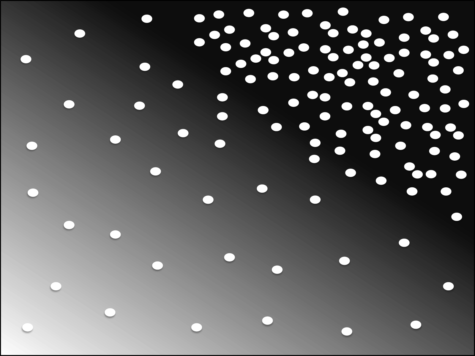
We consider an unbounded domain of fluid initially at rest, as shown in figure 1. This fluid contains a rapidly diffusing scalar, ‘heat’, and the more slowly diffusing ‘sediment’, both of which affect its density in a linear fashion. In the base state, the temperature
 $T(x,z)$
and sediment concentration
 $C(x,z)$
depend linearly on the vertical and horizontal coordinates,
 $z$
and
 $x$
. While the overall density profile is stably stratified, the sediment concentration field by itself is unstably stratified. The horizontal gradients are assumed to be density compensating, so that the overall density of the base state is independent of the horizontal direction.
Schematic of the base state: we consider an overall stably stratified fluid whose density depends on two components. One of them (‘heat’) is stably stratified, while the second one (‘sediment’) is unstably stratified and settles with a constant velocity. The horizontal temperature and sediment concentration gradients are density compensating, so that the base state density profile depends only on the vertical coordinate. Darker shading indicates higher temperature, while the white dots represent sediment grains.

2.1 Governing equations
We analyse the flow based on the two-dimensional Navier–Stokes equations for incompressible flow
 $$\begin{eqnarray}\displaystyle & \displaystyle \unicode[STIX]{x1D735}\boldsymbol{\cdot }\boldsymbol{u}=0, & \displaystyle\end{eqnarray}$$
 $$\begin{eqnarray}\displaystyle & \displaystyle \unicode[STIX]{x1D70C}\left(\frac{\unicode[STIX]{x2202}\boldsymbol{u}}{\unicode[STIX]{x2202}t}+\boldsymbol{u}\boldsymbol{\cdot }\unicode[STIX]{x1D735}\boldsymbol{u}\right)=\unicode[STIX]{x1D707}\unicode[STIX]{x1D6FB}^{2}\boldsymbol{u}-\unicode[STIX]{x1D735}p+(\unicode[STIX]{x1D70C}-\unicode[STIX]{x1D70C}_{m})\boldsymbol{g}, & \displaystyle\end{eqnarray}$$
where
 $\boldsymbol{u}=(u,w)$
indicates the fluid velocity vector,
 $\boldsymbol{g}$
represents the acceleration due to gravity in the
 $-z$
-direction,
 $\unicode[STIX]{x1D707}$
denotes the dynamic viscosity,
 $p$
is the pressure and
 $\unicode[STIX]{x1D70C}_{m}$
indicates a reference density value. The fluid density
 $\unicode[STIX]{x1D70C}$
depends on the temperature and sediment concentration as
 $$\begin{eqnarray}\displaystyle \unicode[STIX]{x1D70C}=\unicode[STIX]{x1D70C}_{m}(1-\unicode[STIX]{x1D6FC}(T-T_{m})+\unicode[STIX]{x1D6FD}(C-C_{m})), & & \displaystyle\end{eqnarray}$$
where
 $(T_{m},C_{m})$
represent reference values for temperature and concentration and the coefficients
 $(\unicode[STIX]{x1D6FC},\unicode[STIX]{x1D6FD})$
reflect the dependence of the density on the temperature and sediment concentration, respectively. Since the density differences in a typical ocean environment are small, we apply the Boussinesq approximation. This allows us to neglect density variations everywhere except in the buoyancy term that drives the fluid motion, so that we can replace
 $\unicode[STIX]{x1D70C}$
on the left-hand side of (2.2) with
 $\unicode[STIX]{x1D70C}_{m}$
.
The temperature and sediment concentration fields are governed by the convection–diffusion transport equations
 $$\begin{eqnarray}\displaystyle & \displaystyle \frac{\unicode[STIX]{x2202}T}{\unicode[STIX]{x2202}t}+\boldsymbol{u}\boldsymbol{\cdot }\unicode[STIX]{x1D735}T=\unicode[STIX]{x1D705}_{T}\unicode[STIX]{x1D6FB}^{2}T, & \displaystyle\end{eqnarray}$$
 $$\begin{eqnarray}\displaystyle & \displaystyle \frac{\unicode[STIX]{x2202}C}{\unicode[STIX]{x2202}t}+\boldsymbol{u}\boldsymbol{\cdot }\unicode[STIX]{x1D735}C-W_{st}^{\ast }\frac{\unicode[STIX]{x2202}C}{\unicode[STIX]{x2202}z}=\unicode[STIX]{x1D705}_{c}\unicode[STIX]{x1D6FB}^{2}C, & \displaystyle\end{eqnarray}$$
where
 $\unicode[STIX]{x1D705}_{T}$
and
 $\unicode[STIX]{x1D705}_{C}$
indicate the thermal and sediment diffusivities, respectively, which are assumed to have constant values, with
 $\unicode[STIX]{x1D705}_{T}>\unicode[STIX]{x1D705}_{C}$
.
 $W_{st}^{\ast }$
represents the constant Stokes settling velocity of the monodisperse sediment.
We will investigate the linear stability of a base state in which the fluid is assumed to be at rest. The temperature and sediment concentration fields of the base state,
 $T_{0}(x,z)$
and
 $C_{0}(x,z,t)$
, depend linearly on the horizontal and vertical directions
 $$\begin{eqnarray}\displaystyle & \displaystyle T_{0}(x,z)=T_{0x}x+T_{0z}z, & \displaystyle\end{eqnarray}$$
 $$\begin{eqnarray}\displaystyle & \displaystyle C_{0}(x,z,t)=C_{0x}x+C_{0z}(z+W_{st}^{\ast }t), & \displaystyle\end{eqnarray}$$
where
 $T_{0x}$
,
 $T_{0z}$
,
 $C_{0x}$
and
 $C_{0z}$
are constants. Since the horizontal temperature and sediment concentration gradients are assumed to be density compensating, we have
 $\unicode[STIX]{x1D6FC}T_{0x}=\unicode[STIX]{x1D6FD}C_{0x}$
. Note that
 $C_{0}$
cannot be constant in time, but must instead have a linear time dependence to account for settling. However, the base state concentration gradients are constant with time.
2.2 Characteristic scales
To non-dimensionalize the governing equations, we adopt the standard characteristic scales of double-diffusive flow as reviewed by Radko (Reference Radko2013). As length scale, we choose the expected finger width
 $$\begin{eqnarray}\displaystyle [d]=\left(\frac{\unicode[STIX]{x1D705}_{T}\unicode[STIX]{x1D708}}{g\unicode[STIX]{x1D6FC}T_{0z}}\right)^{1/4}, & & \displaystyle\end{eqnarray}$$
where
 $\unicode[STIX]{x1D708}=\unicode[STIX]{x1D707}/\unicode[STIX]{x1D70C}_{m}$
denotes the kinematic viscosity and
 $T_{0z}$
represents the magnitude of the base state vertical temperature gradient. Typical values in the mid-latitude thermocline are
 $T_{0z}\sim 0.01\,^{\circ }\text{C}~\text{m}^{-1}$
and
 $d\sim 0.01$
m (Radko Reference Radko2013). As characteristic scales for time, velocity, temperature and sediment concentration, respectively, we obtain
 $$\begin{eqnarray}\displaystyle & \displaystyle [t]=\frac{d^{2}}{\unicode[STIX]{x1D705}_{T}}, & \displaystyle\end{eqnarray}$$
 $$\begin{eqnarray}\displaystyle & \displaystyle [u]=\frac{\unicode[STIX]{x1D705}_{T}}{d}, & \displaystyle\end{eqnarray}$$
 $$\begin{eqnarray}\displaystyle & \displaystyle [T]=T_{0z}d, & \displaystyle\end{eqnarray}$$
 $$\begin{eqnarray}\displaystyle & \displaystyle [C]=\frac{\unicode[STIX]{x1D6FC}}{\unicode[STIX]{x1D6FD}}T_{0z}d. & \displaystyle\end{eqnarray}$$
In this way, we arrive at the following set of governing dimensionless equations for the heat–sediment system
 $$\begin{eqnarray}\displaystyle & \displaystyle \frac{1}{Pr}\left(\frac{\unicode[STIX]{x2202}\boldsymbol{u}}{\unicode[STIX]{x2202}t}+\boldsymbol{u}\boldsymbol{\cdot }\unicode[STIX]{x1D735}\boldsymbol{u}\right)=\unicode[STIX]{x1D6FB}^{2}\boldsymbol{u}-\unicode[STIX]{x1D735}p+(T-C)\hat{\boldsymbol{k}}, & \displaystyle\end{eqnarray}$$
 $$\begin{eqnarray}\displaystyle & \displaystyle \frac{\unicode[STIX]{x2202}T}{\unicode[STIX]{x2202}t}+\boldsymbol{u}\boldsymbol{\cdot }\unicode[STIX]{x1D735}T=\unicode[STIX]{x1D6FB}^{2}T, & \displaystyle\end{eqnarray}$$
 $$\begin{eqnarray}\displaystyle & \displaystyle \frac{\unicode[STIX]{x2202}C}{\unicode[STIX]{x2202}t}+\boldsymbol{u}\boldsymbol{\cdot }\unicode[STIX]{x1D735}C-W_{st}\frac{\unicode[STIX]{x2202}C}{\unicode[STIX]{x2202}z}=\unicode[STIX]{x1D70F}\unicode[STIX]{x1D6FB}^{2}C, & \displaystyle\end{eqnarray}$$
 $$\begin{eqnarray}\displaystyle & \displaystyle \unicode[STIX]{x1D735}\boldsymbol{\cdot }\boldsymbol{u}=0, & \displaystyle\end{eqnarray}$$
whereall quantitieshave now beennon-dimensionalized.The dimensionless parameters in the form of the Prandtl number
 $Pr$
, a diffusivity ratio
 $\unicode[STIX]{x1D70F}$
and a settling velocity
 $W_{st}$
are defined as
 $$\begin{eqnarray}\displaystyle Pr=\frac{\unicode[STIX]{x1D708}}{\unicode[STIX]{x1D705}_{T}},\quad \unicode[STIX]{x1D70F}=\frac{\unicode[STIX]{x1D705}_{C}}{\unicode[STIX]{x1D705}_{T}},\quad W_{st}=\frac{W_{st}^{\ast }d}{\unicode[STIX]{x1D705}_{T}}. & & \displaystyle\end{eqnarray}$$
A further dimensionless quantity arises via the base state in the form of the so-called density ratio
 $R_{\unicode[STIX]{x1D70C}}$
 $$\begin{eqnarray}\displaystyle R_{\unicode[STIX]{x1D70C}}=\frac{\unicode[STIX]{x1D6FC}T_{0z}}{\unicode[STIX]{x1D6FD}C_{0z}}, & & \displaystyle\end{eqnarray}$$
which measures the relative strength of the stabilizing vertical temperature gradient and the destabilizing vertical sediment gradient of the base state (Turner Reference Turner1979).
3 Linear stability analysis
The base state is defined by fluid at rest, along with the dimensionless temperature and sediment concentration fields
 $$\begin{eqnarray}\displaystyle & \displaystyle T_{0}(x,z)=\unicode[STIX]{x1D719}x+z, & \displaystyle\end{eqnarray}$$
 $$\begin{eqnarray}\displaystyle & \displaystyle C_{0}(x,z,t)=\unicode[STIX]{x1D719}x+\frac{1}{R_{\unicode[STIX]{x1D70C}}}(z+W_{st}t). & \displaystyle\end{eqnarray}$$
Here,
 $\unicode[STIX]{x1D719}$
is the slope of lines of constant
 $T_{0}(x,z)$
, defined as
 $$\begin{eqnarray}\displaystyle \unicode[STIX]{x1D719}=\frac{T_{0x}}{T_{0z}}, & & \displaystyle\end{eqnarray}$$
where
 $T_{0x}$
and
 $T_{0z}$
are dimensional values.
In order to conduct a linear stability analysis, we decompose the dimensionless velocity, temperature and sediment fields into their base states and perturbations
 $$\begin{eqnarray}\displaystyle & \displaystyle u(x,z,t)=u^{\prime }(x,z,t), & \displaystyle\end{eqnarray}$$
 $$\begin{eqnarray}\displaystyle & \displaystyle w(x,z,t)=w^{\prime }(x,z,t), & \displaystyle\end{eqnarray}$$
 $$\begin{eqnarray}\displaystyle & \displaystyle T(x,z,t)=T_{0}(x,z)+T^{\prime }(x,z,t), & \displaystyle\end{eqnarray}$$
 $$\begin{eqnarray}\displaystyle & \displaystyle C(x,z,t)=C_{0}(x,z,t)+C^{\prime }(x,z,t), & \displaystyle\end{eqnarray}$$
where
 $u^{\prime }$
,
 $T^{\prime }$
and
 $C^{\prime }$
denote perturbations away from the base state. We assume these perturbations to be small, so that (2.13)–(2.16) can be linearized by neglecting terms that are quadratic in the perturbations. After dropping the primes, we obtain
 $$\begin{eqnarray}\displaystyle & \displaystyle \frac{1}{Pr}\frac{\unicode[STIX]{x2202}u}{\unicode[STIX]{x2202}t}+\frac{\unicode[STIX]{x2202}p}{\unicode[STIX]{x2202}x}-\unicode[STIX]{x1D6FB}^{2}u=0, & \displaystyle\end{eqnarray}$$
 $$\begin{eqnarray}\displaystyle & \displaystyle \frac{1}{Pr}\frac{\unicode[STIX]{x2202}w}{\unicode[STIX]{x2202}t}+\frac{\unicode[STIX]{x2202}p}{\unicode[STIX]{x2202}z}-\unicode[STIX]{x1D6FB}^{2}w+(C-T)=0, & \displaystyle\end{eqnarray}$$
 $$\begin{eqnarray}\displaystyle & \displaystyle \frac{\unicode[STIX]{x2202}T}{\unicode[STIX]{x2202}t}+\unicode[STIX]{x1D719}u+w-\unicode[STIX]{x1D6FB}^{2}T=0, & \displaystyle\end{eqnarray}$$
 $$\begin{eqnarray}\displaystyle & \displaystyle \frac{\unicode[STIX]{x2202}C}{\unicode[STIX]{x2202}t}+\unicode[STIX]{x1D719}u+\frac{1}{R_{\unicode[STIX]{x1D70C}}}w-W_{st}\frac{\unicode[STIX]{x2202}C}{\unicode[STIX]{x2202}z}-\unicode[STIX]{x1D70F}\unicode[STIX]{x1D6FB}^{2}C=0, & \displaystyle\end{eqnarray}$$
 $$\begin{eqnarray}\displaystyle & \displaystyle \frac{\unicode[STIX]{x2202}u}{\unicode[STIX]{x2202}x}+\frac{\unicode[STIX]{x2202}w}{\unicode[STIX]{x2202}z}=0. & \displaystyle\end{eqnarray}$$
The linear stability problem is thus fully defined by the dimensionless parameters
 $Pr$
,
 $\unicode[STIX]{x1D70F}$
,
 $W_{st}$
,
 $\unicode[STIX]{x1D719}$
and
 $R_{\unicode[STIX]{x1D70C}}$
.
We now eliminate the pressure terms by cross-differentiating the momentum equation components, thus obtaining
 $$\begin{eqnarray}\displaystyle \left(\frac{1}{Pr}\frac{\unicode[STIX]{x2202}}{\unicode[STIX]{x2202}t}-\unicode[STIX]{x1D6FB}^{2}\right)\left(\frac{\unicode[STIX]{x2202}u}{\unicode[STIX]{x2202}z}-\frac{\unicode[STIX]{x2202}w}{\unicode[STIX]{x2202}x}\right)+\frac{\unicode[STIX]{x2202}T}{\unicode[STIX]{x2202}x}-\frac{\unicode[STIX]{x2202}C}{\unicode[STIX]{x2202}x}=0. & & \displaystyle\end{eqnarray}$$
This equation describes the generation of vorticity
 $\unicode[STIX]{x1D714}=(\unicode[STIX]{x2202}w/\unicode[STIX]{x2202}x)-(\unicode[STIX]{x2202}u/\unicode[STIX]{x2202}z)$
as a result of horizontal temperature and sediment concentration gradients.
We examine the stability of the system using normal modes of the form
 $$\begin{eqnarray}\displaystyle (u,w,T,C)\sim \text{Re}[(\hat{u} ,{\hat{w}},\hat{T},{\hat{C}})\exp (\unicode[STIX]{x1D706}t+\text{i}lx+\text{i}kz)], & & \displaystyle\end{eqnarray}$$
where
 $\unicode[STIX]{x1D706}=\unicode[STIX]{x1D706}_{R}+\text{i}\unicode[STIX]{x1D706}_{I}$
represents the complex growth rate. The quantities
 $l$
and
 $k$
denote the real horizontal and vertical wavenumbers, respectively, while
 $\hat{u}$
,
 ${\hat{w}}$
,
 $\hat{T}$
and
 ${\hat{C}}$
indicate the amplitudes of the respective Fourier modes. Substitution into the continuity (3.12) gives
 $$\begin{eqnarray}\displaystyle \hat{u} =-\frac{k}{l}{\hat{w}}. & & \displaystyle\end{eqnarray}$$
By substituting the normal modes into (3.13), we obtain
 $$\begin{eqnarray}\displaystyle \left(\frac{\unicode[STIX]{x1D706}}{Pr}+K^{2}\right)(\text{i}k\hat{u} -\text{i}l{\hat{w}})+\text{i}l(\hat{T}-{\hat{C}})=0, & & \displaystyle\end{eqnarray}$$
where
 $K^{2}=l^{2}+k^{2}$
. Further straightforward algebraic manipulations yield the final form of the system as
 $$\begin{eqnarray}\displaystyle & \displaystyle \left(\frac{\unicode[STIX]{x1D706}}{Pr}+K^{2}\right)\left(\frac{K^{2}}{l^{2}}\right){\hat{w}}=(\hat{T}-{\hat{C}}), & \displaystyle\end{eqnarray}$$
 $$\begin{eqnarray}\displaystyle & \displaystyle (\unicode[STIX]{x1D706}+K^{2})\hat{T}=\left(\frac{\unicode[STIX]{x1D719}k}{l}-1\right){\hat{w}}, & \displaystyle\end{eqnarray}$$
 $$\begin{eqnarray}\displaystyle & \displaystyle (\unicode[STIX]{x1D706}+\unicode[STIX]{x1D70F}K^{2}-W_{st}\text{i}k){\hat{C}}=\left(\frac{\unicode[STIX]{x1D719}k}{l}-\frac{1}{R_{\unicode[STIX]{x1D70C}}}\right){\hat{w}}. & \displaystyle\end{eqnarray}$$
These equations can be combined into a single cubic expression for the complex growth rate
 $$\begin{eqnarray}\displaystyle \unicode[STIX]{x1D706}^{3}+a_{2}\unicode[STIX]{x1D706}^{2}+a_{1}\unicode[STIX]{x1D706}+a_{0}=0, & & \displaystyle\end{eqnarray}$$
where
 $$\begin{eqnarray}\displaystyle & \displaystyle a_{2}=K^{2}(1+Pr+\unicode[STIX]{x1D70F})-\text{i}W_{st}k, & \displaystyle\end{eqnarray}$$
 $$\begin{eqnarray}\displaystyle & \displaystyle a_{1}=K^{4}(\unicode[STIX]{x1D70F}+Pr+\unicode[STIX]{x1D70F}Pr)+Pr\frac{l^{2}}{K^{2}}\left(1-\frac{1}{R_{\unicode[STIX]{x1D70C}}}\right)-\text{i}K^{2}W_{st}k(1+Pr), & \displaystyle\end{eqnarray}$$
 $$\begin{eqnarray}\displaystyle & \displaystyle a_{0}=\unicode[STIX]{x1D70F}PrK^{6}+Prl^{2}\left(\unicode[STIX]{x1D70F}-\frac{1}{R_{\unicode[STIX]{x1D70C}}}\right)+Prlk\unicode[STIX]{x1D719}(1-\unicode[STIX]{x1D70F})+\frac{\text{i}PrW_{st}k}{K^{2}}(\unicode[STIX]{x1D719}lk-l^{2}-K^{6}). & \displaystyle\end{eqnarray}$$
In contrast to the traditional thermohaline double-diffusive system, the coefficients in the above cubic equation for the heat–sediment system are complex, as a result of the settling velocity term in the governing equations. When
 $W_{st}=0$
, our cubic system reduces to the one obtained by Holyer (Reference Holyer1983). When
 $\unicode[STIX]{x1D719}=0$
, we recover the results of Reali et al. (Reference Reali, Garaud, Alsinan and Meiburg2017).
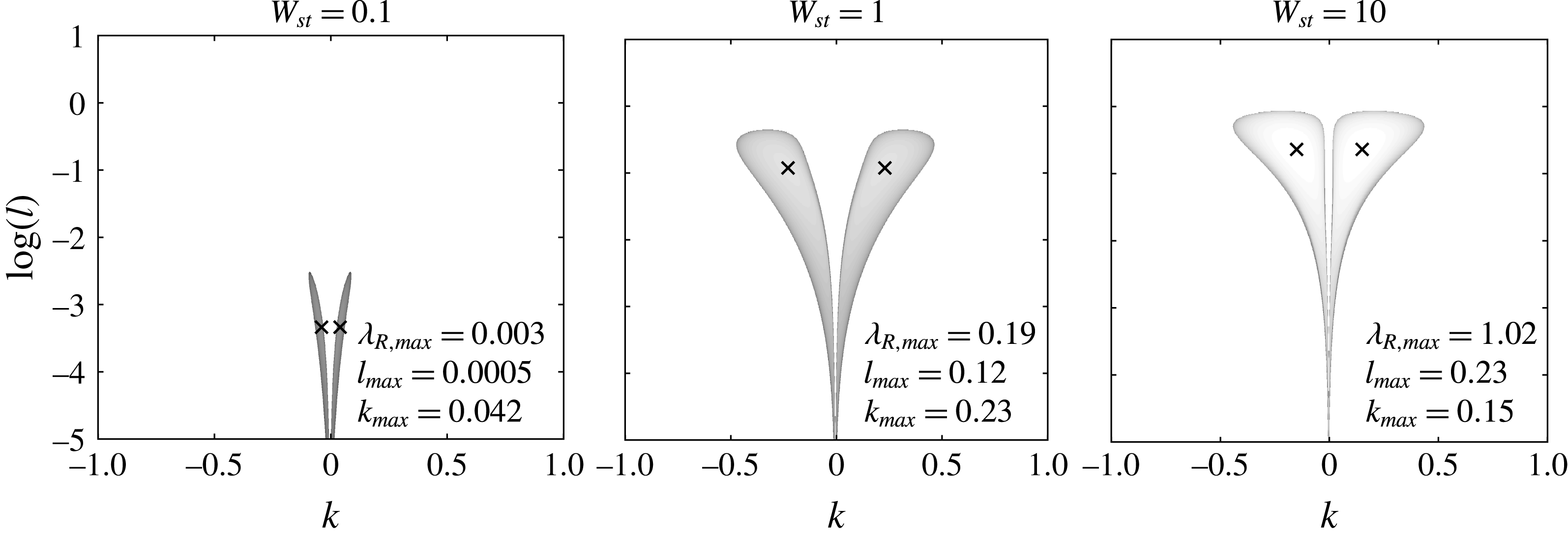
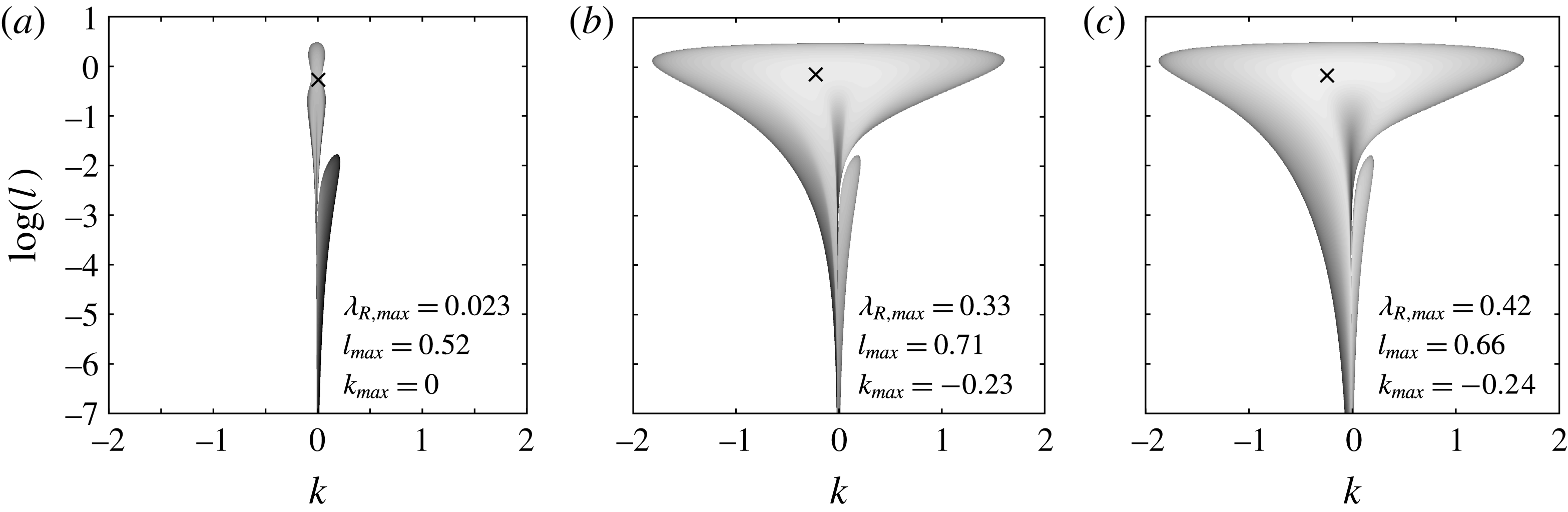
 $Pr=7$
,
 $\unicode[STIX]{x1D70F}=1$
,
 $R_{\unicode[STIX]{x1D70C}}=1.5$
,
 $\unicode[STIX]{x1D719}=0$
: maximum real part
 $\unicode[STIX]{x1D706}_{R}$
of the growth rate as function of the vertical (
 $k$
) and horizontal (
 $l$
) wavenumbers, for three different values of the particle settling velocity
 $W_{st}$
. Only positive values of
 $\unicode[STIX]{x1D706}_{R}$
are shown, and the mode with the largest growth rate
 $\unicode[STIX]{x1D706}_{R,max}$
is marked with an ‘
 $\times$
’. The grey shading is scaled to
 $\log (\unicode[STIX]{x1D706}_{R})$
. Since the two scalars have equal diffusivities (
 $\unicode[STIX]{x1D70F}=1$
), the system is stable with regard to double diffusion, and the instability is driven purely by settling. The dominant mode has the shape of inclined waves, and both the maximum growth rate
 $\unicode[STIX]{x1D706}_{R,max}$
and the unstable wavenumber range increase with
 $W_{st}$
.

In the following, we will analyse solutions of the above system, in terms of both growth rates and eigenfunctions.
4 Results
4.1 Settling-driven instability
4.1.1 Growth rate
In order to clarify the role of settling, we begin by discussing the idealized case without double-diffusive instabilities (
 $\unicode[STIX]{x1D70F}=1$
), which is well known to be stable in the absence of settling. Figure 2 demonstrates that non-zero settling velocities drive instabilities, in spite of the overall stable density stratification. To the best of our knowledge, this purely settling-driven instability has not been reported before. The figure displays the maximum value of the real part of the growth rate,
 $\unicode[STIX]{x1D706}_{R}$
, as a function of the horizontal and vertical wavenumbers
 $l$
and
 $k$
, for three different values of the settling velocity
 $W_{st}$
. The other parameter values are held fixed at
 $Pr=7$
,
 $\unicode[STIX]{x1D70F}=1$
,
 $R_{\unicode[STIX]{x1D70C}}=1.5$
and
 $\unicode[STIX]{x1D719}=0$
, so that there are no lateral base state gradients. We observe the existence of two symmetric, lobe-shaped unstable regions for
 $k>0$
and
 $k<0$
, while the ‘elevator’ mode
 $k=0$
is always stable. The maximum growth rate
 $\unicode[STIX]{x1D706}_{R,max}$
is seen to increase with
 $W_{st}$
.
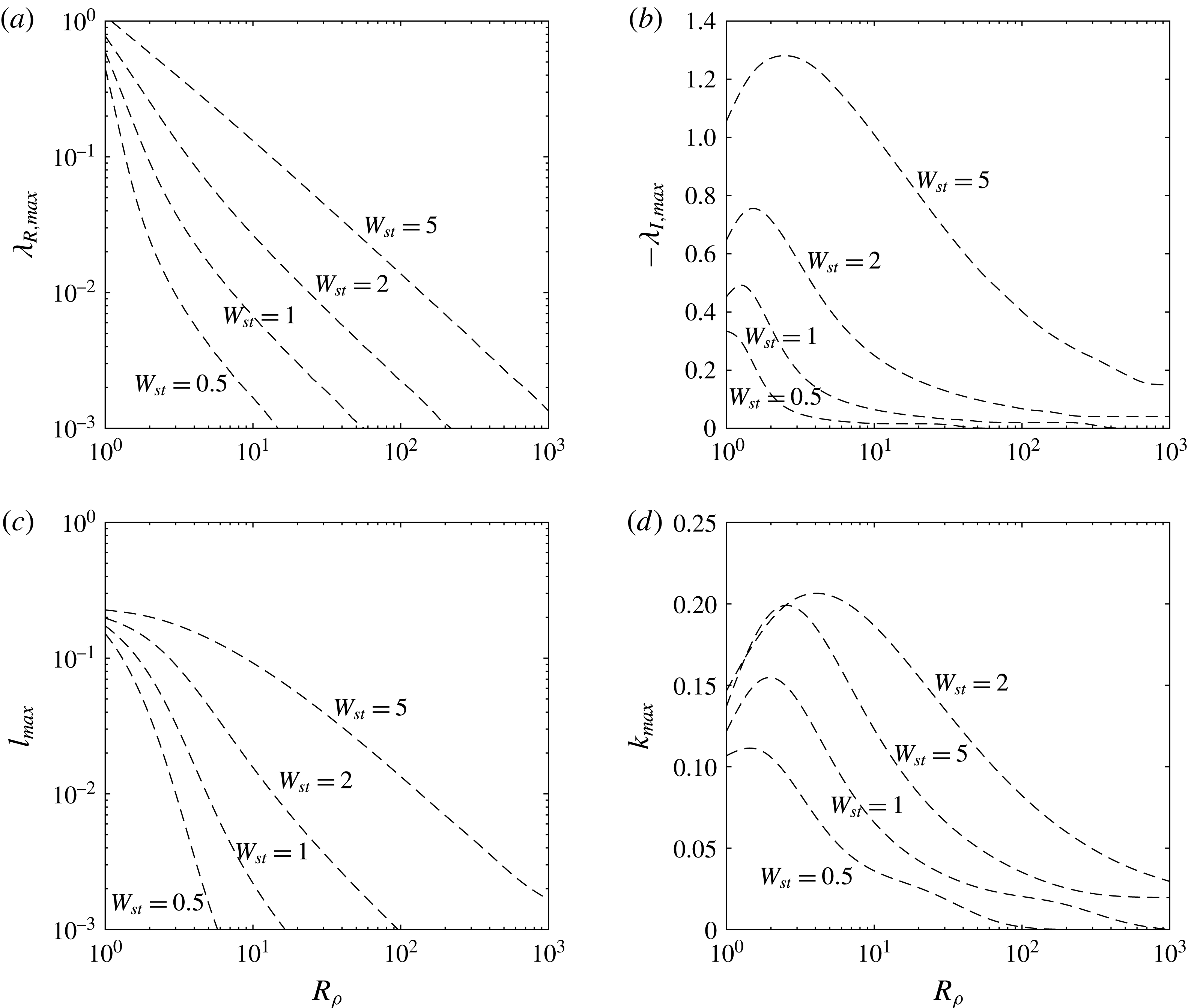
Figure 3 demonstrates that this settling-driven instability can be present for all values of the density ratio
 $R_{\unicode[STIX]{x1D70C}}$
, although the growth rate decreases with increasing
 $R_{\unicode[STIX]{x1D70C}}$
. The horizontal wavelength of the dominant mode grows monotonically with
 $R_{\unicode[STIX]{x1D70C}}$
and decreases for larger
 $W_{st}$
, while its vertical wavenumber is seen to peak at intermediate values of
 $R_{\unicode[STIX]{x1D70C}}$
.
 $Pr=7$
,
 $\unicode[STIX]{x1D70F}=1$
,
 $\unicode[STIX]{x1D719}=0$
: dependence of the dominant mode properties on the density ratio
 $R_{\unicode[STIX]{x1D70C}}$
, for selected values of the settling velocity
 $W_{st}$
. Since double diffusion is absent, the instability is driven purely by settling, and the case
 $W_{st}=0$
is stable. (a) The maximum growth rate
 $\unicode[STIX]{x1D706}_{R,max}$
increases uniformly with
 $W_{st}$
, and decreases monotonically for larger values of
 $R_{\unicode[STIX]{x1D70C}}$
. (b) The imaginary part
 $\unicode[STIX]{x1D706}_{I,max}$
of the growth rate of the dominant mode. This mode has the form of a downward travelling inclined wave. (c) The horizontal wavenumber
 $l_{max}$
of the dominant mode increases with
 $W_{st}$
but decreases with
 $R_{\unicode[STIX]{x1D70C}}$
. (d) The vertical wavenumber
 $k_{max}$
of the dominant mode increases with
 $W_{st}$
, and peaks for intermediate density ratios.

4.1.2 Eigenfunctions
Key to understanding the mechanism driving this new instability is (3.13), which states that vorticity is produced as a result of horizontal gradients in the temperature and sediment concentration fields. Equation (3.13) allows us to develop a vorticity-based physical interpretation of the linear stability behaviour in the presence of horizontal temperature and sediment concentration perturbations. Since the base state temperature profile is stably stratified, the vorticity generated as a result of
 $\unicode[STIX]{x2202}T/\unicode[STIX]{x2202}x$
(the ‘
 $T$
-vorticity’) is of such a sign that it wants to return the flow to the base state. Hence we refer to the
 $T$
-vorticity as being stabilizing. This is in contrast to any vorticity generated by
 $\unicode[STIX]{x2202}C/\unicode[STIX]{x2202}x$
(the ‘
 $C$
-vorticity’), which wants to move the flow further away from the base state and hence is destabilizing. Comparing the strength of the stabilizing
 $T$
-vorticity to the destabilizing
 $C$
-vorticity will hence allow us to gain insight into the overall stability of the flow. As a consequence of the characteristic temperature and concentration scales introduced above, static stability of the base profile implies
 $R_{\unicode[STIX]{x1D70C}}>1$
. Hence, in the absence of diffusion and settling, any convective distortion of the base profile will result in
 $|\unicode[STIX]{x2202}T/\unicode[STIX]{x2202}x|>|\unicode[STIX]{x2202}C/\unicode[STIX]{x2202}x|$
everywhere. Consequently, equation (3.13) states that the stabilizing
 $T$
-vorticity always outweighs the destabilizing
 $C$
-vorticity at the same location, so that the overall system is stable. In the present context, there exist two potential scenarios for modifying the balance between the stabilizing
 $T$
-vorticity and the destabilizing
 $C$
-vorticity. First, double diffusion can render the flow unstable by smoothing out
 $\unicode[STIX]{x2202}T/\unicode[STIX]{x2202}x$
-gradients more rapidly than
 $\unicode[STIX]{x2202}C/\unicode[STIX]{x2202}x$
-gradients, so that the destabilizing
 $C$
-vorticity outweighs the stabilizing
 $T$
-vorticity in the same location. In addition there is the second possibility that the presence of a settling velocity for the sediment concentration field can shift the corresponding
 $T$
- and
 $C$
-contours relative to each other, so that the stabilizing
 $T$
-vorticity may no longer be able to overcome the destabilizing
 $C$
-vorticity everywhere, which again can render the overall system unstable. Both of these scenarios are discussed below.
In order to understand why the presence of the settling velocity destabilizes inclined waves
 $k\neq 0$
, but not the elevator mode
 $k=0$
, we examine the eigenfunctions of the velocity components, vorticity, temperature and sediment concentration
 $$\begin{eqnarray}\displaystyle \left(\begin{array}{@{}c@{}}w\\ u\\ \unicode[STIX]{x1D714}\\ T\\ C\end{array}\right)=\text{Re}\left[\left(\begin{array}{@{}c@{}}{\hat{w}}\\ \displaystyle -\frac{k}{l}{\hat{w}}\\ \displaystyle \frac{(l^{2}+k^{2})\text{i}}{l}{\hat{w}}\\ \hat{T}\\ {\hat{C}}\end{array}\right)\text{e}^{\text{i}lx+\text{i}kz}\right] & & \displaystyle\end{eqnarray}$$
in light of this vorticity-based physical interpretation. For
 $k=0$
, the temperature and sediment perturbations do not depend on the vertical
 $z$
-coordinate, so that they are not modified by vertical advection due to settling. Hence the elevator mode, which is stable for
 $\unicode[STIX]{x1D70F}=1$
in the absence of settling, remains stable when a settling velocity is present. For modes with
 $k\neq 0$
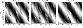
, on the other hand, a different picture emerges, cf. figure 4. Compared to the inclined temperature contours, the contours of the sediment concentration field are now shifted downward by the settling velocity, so that at a constant
 $z$
-location a horizontal phase shift emerges between the temperature and sediment concentration contours, and hence between the stabilizing
 $T$
- and the destabilizing
 $C$
-vorticity. Consequently, the stabilizing
 $T$
-vorticity can no longer overcome the destabilizing
 $C$
-vorticity everywhere, so that inclined modes with
 $k\neq 0$
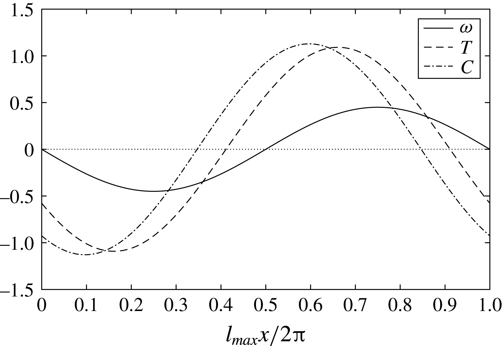
are destabilized. This picture is confirmed by figure 5, which shows the two-dimensional unstable eigenmodes for temperature, sediment concentration and vorticity, together with the superimposed velocity vectors.
 $Pr=7$
,
 $\unicode[STIX]{x1D70F}=1$
,
 $R_{\unicode[STIX]{x1D70C}}=1.5$
,
 $\unicode[STIX]{x1D719}=0$
,
 $W_{st}=2$
: horizontal cross-cut of the normalized two-dimensional dominant mode eigenfunctions for vorticity
 $\unicode[STIX]{x1D714}$
, temperature
 $T$
and sediment concentration
 $C$
. Since the dominant mode has the form of an inclined wave, the settling velocity of the sediment concentration field results in a horizontal phase shift between the
 $T$
- and
 $C$
-waves. This translates into a phase shift between the stabilizing and destabilizing vorticity waves associated with these two scalars, which in turn causes the instability.

 $Pr=7$
,
 $\unicode[STIX]{x1D70F}=1$
,
 $R_{\unicode[STIX]{x1D70C}}=1.5$
,
 $\unicode[STIX]{x1D719}=0$
,
 $W_{st}=10$
: two-dimensional dominant mode eigenfunctions of temperature
 $T$
, sediment concentration
 $C$
and vorticity
 $\unicode[STIX]{x1D714}$
, for the case of a purely settling-driven instability. Superimposed are the velocity vectors corresponding to the
 $u$
- and
 $w$
-eigenfunctions. The horizontal and vertical axes are normalized by the size of the region shown, which is 50. Note the slight phase shift between the
 $C$
- and
 $T$
-eigenfunctions, which is responsible for the instability.

 $Pr=7$
,
 $\unicode[STIX]{x1D70F}=0.01$
,
 $R_{\unicode[STIX]{x1D70C}}=1.5$
,
 $\unicode[STIX]{x1D719}=0$
: maximum real part
 $\unicode[STIX]{x1D706}_{R}$
of the growth rate as function of the vertical (
 $k$
) and horizontal (
 $l$
) wavenumbers, for three different values of the particle settling velocity
 $W_{st}$
. Only positive values of
 $\unicode[STIX]{x1D706}_{R}$
are shown, and the mode with the largest growth rate
 $\unicode[STIX]{x1D706}_{R,max}$
is marked with an ‘
 $\times$
’. The grey shading is scaled to
 $\log (\unicode[STIX]{x1D706}_{R})$
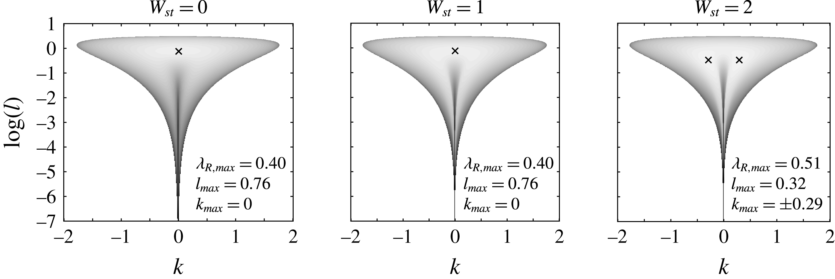
. For
 $W_{st}=0$
, only the double-diffusive instability is active, and the most unstable mode is of elevator type. While the presence of a settling velocity does not modify the elevator mode, it destabilizes inclined waves. Beyond a critical value of
 $W_{st}$
, the dominant mode takes the shape of inclined waves with
 $k\neq 0$
.

4.2 Influence of double diffusion
We now proceed to systems with
 $\unicode[STIX]{x1D70F}\neq 1$
and
 $W_{st}\neq 0$
, in order to study the interaction of settling-driven and double-diffusive instabilities. In the following, our discussion will focus primarily on the effects of the settling velocity
 $W_{st}$
under these conditions, with the remaining dimensionless parameters held fixed at
 $Pr=7$
,
 $\unicode[STIX]{x1D70F}=0.01$
,
 $R_{\unicode[STIX]{x1D70C}}=1.5$
and
 $\unicode[STIX]{x1D719}=0$
, unless stated otherwise. Figure 6 shows the maximum value of the real part of the growth rate,
 $\unicode[STIX]{x1D706}_{R}$
, as function of the horizontal and vertical wavenumbers
 $l$
and
 $k$
, for three different values of the settling velocity
 $W_{st}$
. Only unstable solutions
 $\unicode[STIX]{x1D706}_{R}>0$
are shown, and the mode with the largest growth rate
 $\unicode[STIX]{x1D706}_{R,max}$
is again marked by an ‘
 $\times$
’. Consistent with earlier results, e.g. Baines & Gill (Reference Baines and Gill1969), we find that for the case of purely double-diffusive instability (
 $W_{st}=0$
) the most unstable mode has a vertical wavenumber
 $k=0$
. For moderate settling velocities, e.g.
 $W_{st}=1$
, fingering remains the dominant mode, and neither the most unstable horizontal wavenumber
 $l_{max}$
nor the value of
 $\unicode[STIX]{x1D706}_{R,max}$
vary as a function of
 $W_{st}$
. This is consistent with our argument above that a settling velocity does not affect perturbations associated with the elevator mode.
 $Pr=7$
,
 $\unicode[STIX]{x1D70F}=0.01$
,
 $R_{\unicode[STIX]{x1D70C}}=1.5$
,
 $\unicode[STIX]{x1D719}=0$
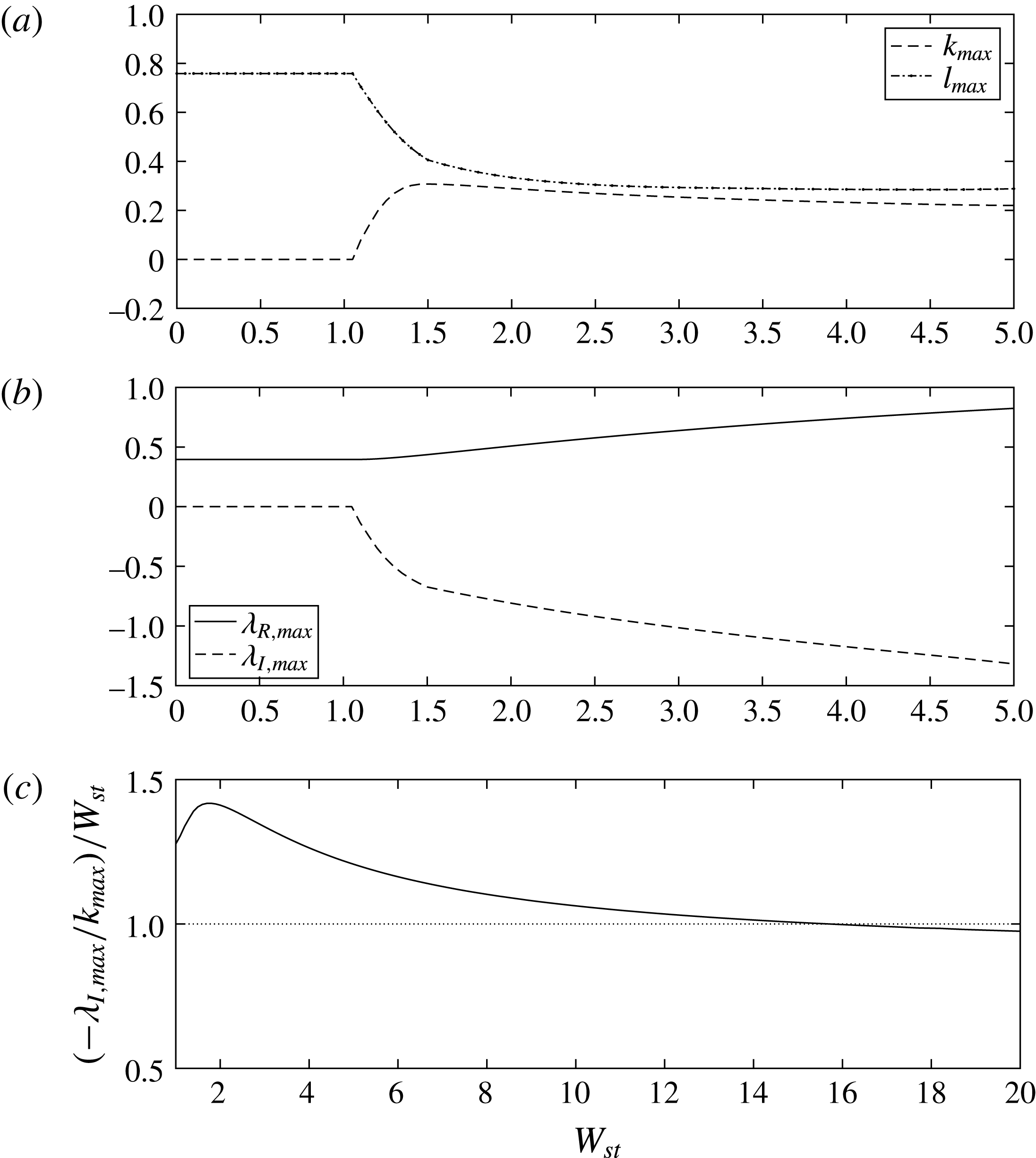
: (a) most unstable horizontal (
 $l_{max}$
) and vertical (
 $k_{max}$
) wavenumbers as functions of the particle settling velocity
 $W_{st}$
. Beyond the critical value of the settling velocity
 $(W_{st,crit}\approx 1.05)$
, settling-driven inclined waves overtake those of the double-diffusive elevator mode as the dominant instability mode. (b) Beyond
 $W_{st,crit}$
, the growth rate
 $\unicode[STIX]{x1D706}_{R,max}$
of the dominant mode increases uniformly with
 $W_{st}$
, while the imaginary part of the growth rate
 $\unicode[STIX]{x1D706}_{I,max}$
deviates from zero. (c) The ratio of the vertical phase velocity of the dominant mode
 $\unicode[STIX]{x1D706}_{I,max}/k_{max}$
to the particle settling velocity. For large
 $W_{st}$
this ratio approaches one, showing that the wave travels approximately with the particle settling velocity.

Once the settling velocity exceeds a critical value of
 $W_{st,crit}\approx 1.05$
, this picture changes, as the growth rates of modes with
 $k\neq 0$
overtake the elevator mode. For successively larger values of
 $W_{st}$
, the most amplified horizontal wavenumber decreases, while its growth rate
 $\unicode[STIX]{x1D706}_{R,max}$
increases. The above observation is confirmed by figure 7, which demonstrates that at the critical value of
 $W_{st}$
the dominant instability mode switches from
 $k_{max}=0$
to
 $k_{max}\neq 0$
. For the present parameter combination, the horizontal and vertical wavenumbers of the dominant mode are similar in magnitude for
 $W_{st}$
-values above approximately 1.5, so that its wavefronts are inclined at roughly
 $45^{\circ }$
. The growth rate
 $\unicode[STIX]{x1D706}_{R,max}$
of the dominant mode increases monotonically with
 $W_{st}$
, while
 $\unicode[STIX]{x1D706}_{I,max}$
decreases.
Figure 7(c) displays the ratio of the downward vertical velocity
 $-\unicode[STIX]{x1D706}_{I,max}/k_{max}$
of the most unstable mode to the settling velocity
 $W_{st}$
. We find that beyond the critical value of
 $W_{st,crit}\approx 1.05$
the downward velocity of the most unstable mode tends towards the particle settling velocity
 $W_{st}$
, so that the ratio
 $-\unicode[STIX]{x1D706}_{I,max}/(W_{st}k_{max})$
approaches unity.
4.3 Influence of the density ratio
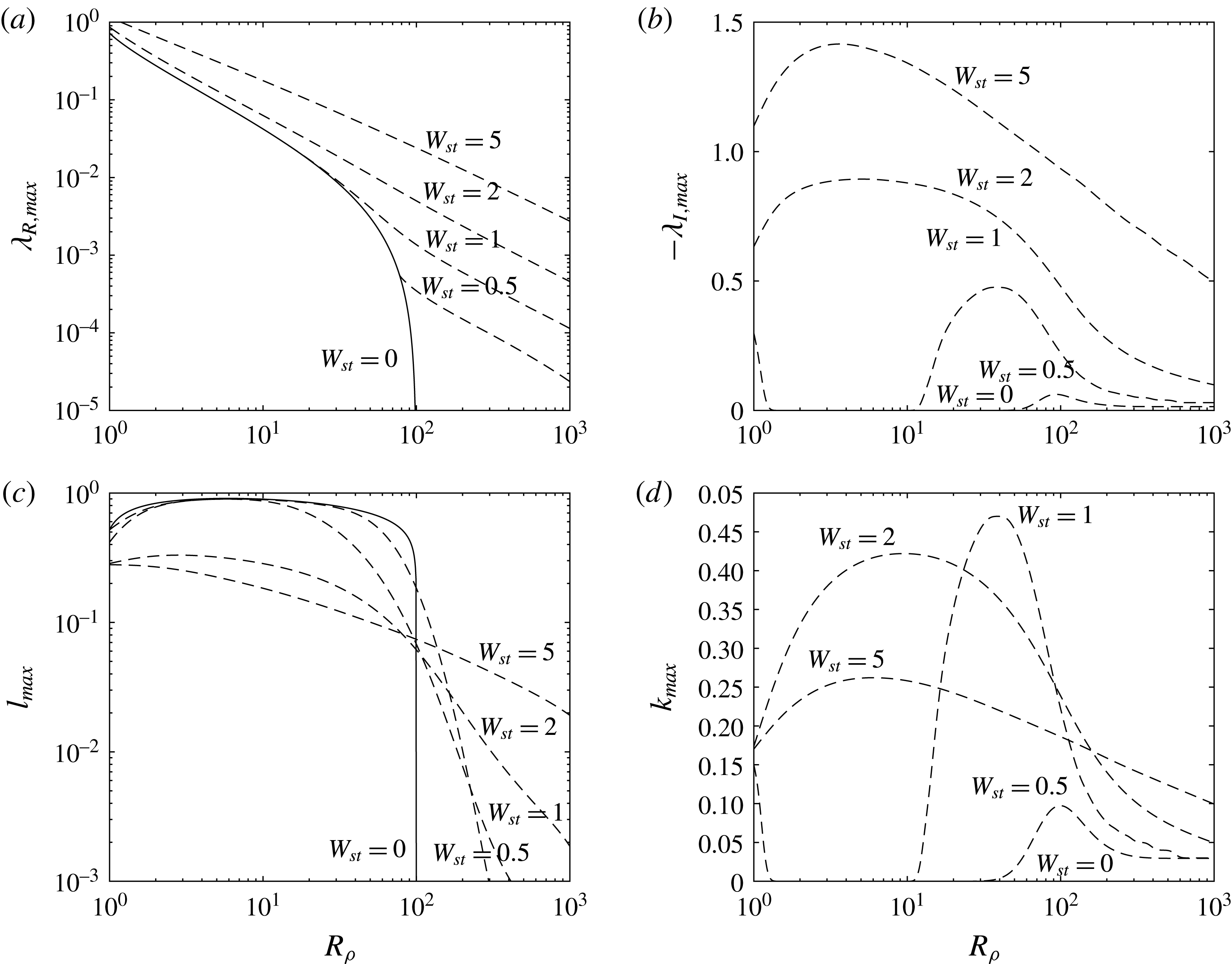
 $Pr=7$
,
 $\unicode[STIX]{x1D70F}=0.01$
,
 $\unicode[STIX]{x1D719}=0$
: variation of the dominant mode properties with the density ratio
 $R_{\unicode[STIX]{x1D70C}}$
and the settling velocity
 $W_{st}$
, when both double-diffusive and settling-driven instabilities are present. (a) The maximum growth rate
 $\unicode[STIX]{x1D706}_{R,max}$
: for
 $W_{st}=0$
, only the double-diffusive instability is present, so that only density ratios
 $\unicode[STIX]{x1D70F}<1/R_{\unicode[STIX]{x1D70C}}$
are unstable. For
 $W_{st}>0$
the settling-driven mode destabilizes all density ratios. (b) The imaginary part
 $\unicode[STIX]{x1D706}_{I,max}$
of the growth rate: for small values of
 $W_{st}$
and
 $R_{\unicode[STIX]{x1D70C}}<1/\unicode[STIX]{x1D70F}$
, the dominant mode is of elevator type. (c) For large density ratios, the horizontal wavenumber
 $l_{max}$
of the dominant mode decreases with
 $R_{\unicode[STIX]{x1D70C}}$
. (d) The vertical wavenumber
 $k_{max}$
of the dominant mode peaks for intermediate density ratios.

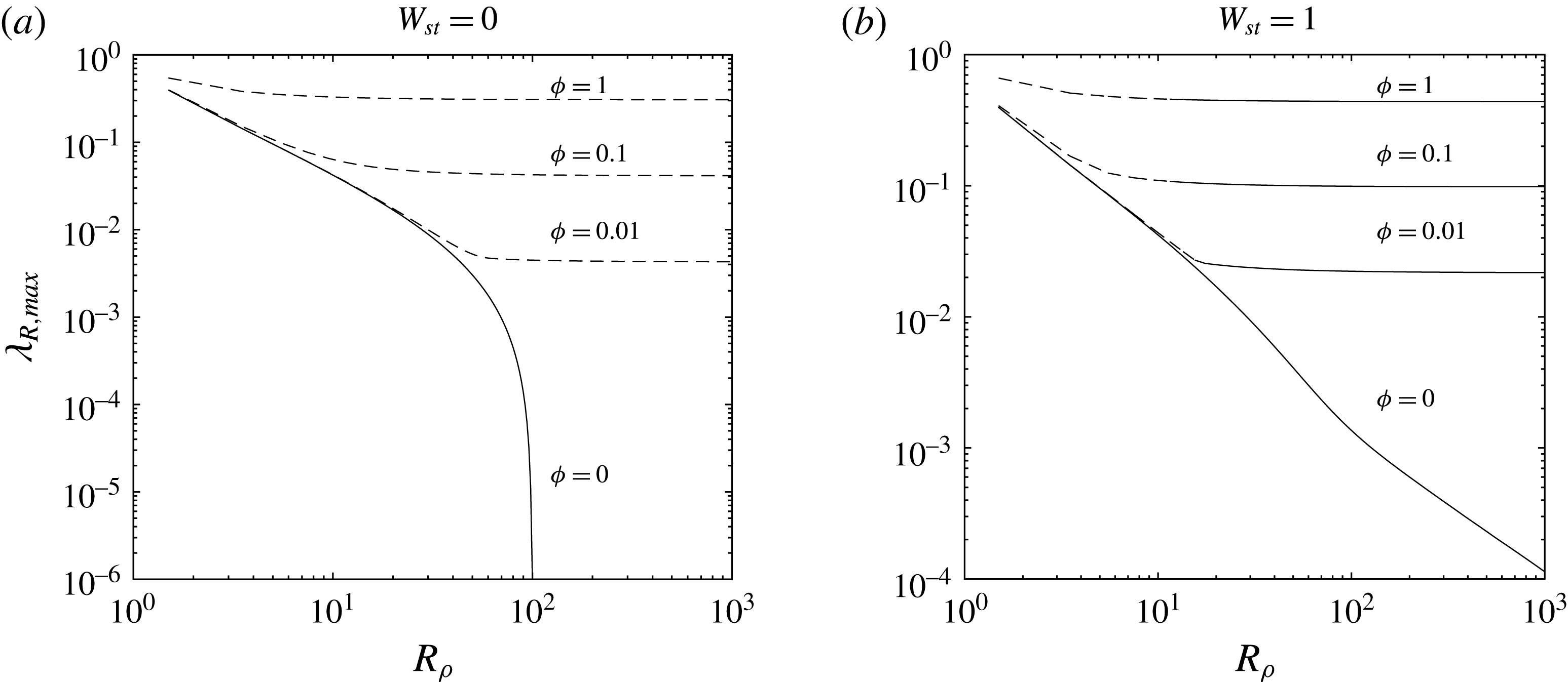
Figure 8(a), which is similar to a corresponding figure in Reali et al. (Reference Reali, Garaud, Alsinan and Meiburg2017) albeit for different parameters, analyses the influence of the density ratio on the heat–sediment system in the absence of lateral base state gradients. For vanishing settling velocity
 $W_{st}=0$
, we confirm the well-known result that only density ratios
 $R_{\unicode[STIX]{x1D70C}}<1/\unicode[STIX]{x1D70F}$
are unstable. A positive settling velocity
 $W_{st}>0$
, on the other hand, immediately destabilizes all density ratios
 $R_{\unicode[STIX]{x1D70C}}>1/\unicode[STIX]{x1D70F}$
as well. This destabilizing effect grows with the settling velocity. For a given value of
 $R_{\unicode[STIX]{x1D70C}}<1/\unicode[STIX]{x1D70F}$
, the growth rate is affected by the settling velocity only above a critical value of
 $W_{st}$
, which is consistent with the results of § 4.2. This critical value of
 $W_{st}$
decreases for larger density ratios. Within the regime where the growth rate is affected by the settling velocity, visual inspection indicates a power-law dependence of
 $\unicode[STIX]{x1D706}_{R,max}$
on
 $R_{\unicode[STIX]{x1D70C}}$
 $$\begin{eqnarray}\displaystyle \unicode[STIX]{x1D706}_{R,max}\propto R_{\unicode[STIX]{x1D70C}}^{-n}, & & \displaystyle\end{eqnarray}$$
where
 $n\approx 1$
.
Figure 8(b–d) shows corresponding results for
 $\unicode[STIX]{x1D706}_{I,max}$
,
 $l_{max}$
and
 $k_{max}$
. For small values of
 $W_{st}$
and
 $R_{\unicode[STIX]{x1D70C}}<1/\unicode[STIX]{x1D70F}$
, where the instability growth rate
 $\unicode[STIX]{x1D706}_{R,max}$
is independent of the settling velocity, both
 $\unicode[STIX]{x1D706}_{I,max}$
and
 $k_{max}$
are identically zero, so that the dominant instability mode is elevator like and does not travel in the vertical direction. For larger
 $W_{st}$
-values, on the other hand, inclined modes dominate across the entire
 $R_{\unicode[STIX]{x1D70C}}$
range. The intermediate value of
 $W_{st}=1$
gives rise to three different regimes: near
 $R_{\unicode[STIX]{x1D70C}}\approx 1$
inclined waves are most amplified, for
 $1.14\leqslant R_{\unicode[STIX]{x1D70C}}\leqslant 10$
the elevator mode dominates and beyond that inclined modes are once again most unstable. Figure 8(c) demonstrates that for
 $R_{\unicode[STIX]{x1D70C}}>1/\unicode[STIX]{x1D70F}$
, larger values of
 $W_{st}$
tend to favour shorter horizontal wavelengths.
4.4 Influence of the diffusivity ratio
 $Pr=7$
,
 $R_{\unicode[STIX]{x1D70C}}=1.5$
,
 $\unicode[STIX]{x1D719}=0$
: variation of the dominant mode properties with the diffusivity ratio
 $\unicode[STIX]{x1D70F}$
and the settling velocity
 $W_{st}$
. For
 $W_{st}=0$
, double-diffusive fingering exists below
 $\unicode[STIX]{x1D70F}<1/R_{\unicode[STIX]{x1D70C}}$
, and oscillatory double diffusion with
 $\unicode[STIX]{x1D706}_{I,max}>0$
is seen for
 $\unicode[STIX]{x1D70F}\geqslant 5$
. For
 $W_{st}>0$
the intermediate
 $\unicode[STIX]{x1D70F}$
-range becomes destabilized as well, with regard to downward travelling, inclined waves. Consequently, in the presence of settling the flow is unstable for all values of
 $\unicode[STIX]{x1D70F}$
.

An interesting picture emerges when we analyse the influence of the diffusivity ratio on the stability of the system for
 $Pr=7$
,
 $R_{\unicode[STIX]{x1D70C}}=1.5$
,
 $\unicode[STIX]{x1D719}=0$
and various values of the settling velocity
 $W_{st}$
, cf. figure 9. In the absence of settling, the regime
 $\unicode[STIX]{x1D70F}<1/R_{\unicode[STIX]{x1D70C}}$
is unstable to traditional double-diffusive fingering, with
 $\unicode[STIX]{x1D706}_{I,max}=0$
. For
 $\unicode[STIX]{x1D70F}\geqslant 5$
, we observe the well-known oscillatory ‘diffusive’ instability regime with
 $\unicode[STIX]{x1D706}_{I,max}>0$
. Without settling, the range in between these two
 $\unicode[STIX]{x1D70F}$
-values is stable, with
 $\unicode[STIX]{x1D706}_{I,max}<0$
. In the presence of settling, this intermediate
 $\unicode[STIX]{x1D70F}$
-range becomes unstable to inclined waves, with larger settling velocities resulting in higher growth rates. Hence in the presence of settling the flow is unstable for all
 $\unicode[STIX]{x1D70F}$
-values. This indicates that the system develops instabilities even if the unstably stratified ‘sediment’ component diffuses more rapidly than the stably stratified ‘temperature’ component, which may occur for certain sediment grain sizes (Reali et al.
Reference Reali, Garaud, Alsinan and Meiburg2017). Figure 9 furthermore indicates that for the traditional fingering regime
 $\unicode[STIX]{x1D70F}<1/R_{\unicode[STIX]{x1D70C}}$
the critical value of
 $W_{st}$
depends on
 $\unicode[STIX]{x1D70F}$
.
4.5 Influence of lateral gradients
 $Pr=7$
,
 $\unicode[STIX]{x1D70F}=0.01$
,
 $R_{\unicode[STIX]{x1D70C}}=1.5$
,
 $\unicode[STIX]{x1D719}=0.1$
,
 $W_{st}=0$
: (a) maximum real part
 $\unicode[STIX]{x1D706}_{R}$
of the growth rate as function of the vertical (
 $k$
) and horizontal (
 $l$
) wavenumbers: a lateral base state gradient breaks the symmetry, by shifting the dominant double-diffusive fingering mode to
 $k_{max}<0$
. At the same time, a new intrusive instability mode appears for small
 $k$
and
 $l$
. (b) Contours of the base state temperature field. (c) The vorticity eigenfunction for the dominant fingering mode with
 $l=0.76$
and
 $k=-0.09$
. (d) The vorticity eigenfunction for the intrusive mode. Note that the wavefronts for the fingering and intrusive modes are inclined in opposite directions.

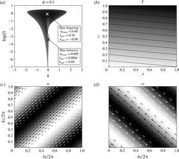
Lateral gradients break the overall symmetry of the system with regard to
 $k=0$
, as shown in figure 10(a). As we introduce a lateral gradient of
 $\unicode[STIX]{x1D719}=0.1$
, the dominant mode in the absence of settling switches from
 $k=0$
to
 $k<0$
. Figure 10(b) shows the inclined temperature base state, which is density compensated by a corresponding sediment concentration field, so that all base state density contours are horizontal. Figure 10(c) displays the vorticity eigenfunction for the most unstable mode with
 $l=0.76$
and
 $k=-0.09$
. We find that its wavefronts are tilted in the opposite direction from the base state temperature and sediment concentration contours. At the same time, a new instability mode in the shape of a small ‘leaf’ appears for
 $k>0$
and large horizontal wavelengths in the lower right quadrant of figure 10(a). This unstable region represents the intrusive mode discussed by Medrano et al. (Reference Medrano, Garaud and Stellmach2014). Its perturbation wavefronts are tilted in the same direction as the base state temperature and sediment concentration contours, as can be seen in figure 10(d).
By generating plots similar to figure 10(a), but for different values of
 $W_{st}$
, we can analyse how these two distinct instability modes are affected by settling. We find that the growth rate of the dominant fingering mode increases with the settling velocity, and its horizontal wavelength increases. The intrusion mode initially becomes more prominent as
 $W_{st}$
increases, but beyond
 $W_{st}\approx 1$
the shape of its lobe varies only weakly with
 $W_{st}$
.
 $Pr=7$
,
 $\unicode[STIX]{x1D70F}=0.01$
: variation of the growth rate
 $\unicode[STIX]{x1D706}_{R,max}$
of the dominant mode with the density ratio
 $R_{\unicode[STIX]{x1D70C}}$
and the lateral base state gradient
 $\unicode[STIX]{x1D719}$
, for two different values of
 $W_{st}$
. A lateral base state gradient
 $\unicode[STIX]{x1D719}>0$
destabilizes the flow for all density ratios
 $R_{\unicode[STIX]{x1D70C}}$
. A settling velocity
 $W_{st}>0$
also destabilizes
 $\unicode[STIX]{x1D719}=0$
.

Figure 11(a) confirms the earlier observation by Holyer (Reference Holyer1983) that, in the absence of a settling velocity, lateral base state gradients destabilize the flow for all density ratios
 $R_{\unicode[STIX]{x1D70C}}$
. In the regime
 $R_{\unicode[STIX]{x1D70C}}<1/\unicode[STIX]{x1D70F}$
, which is unstable even in the absence of lateral base state gradients, the influence of
 $\unicode[STIX]{x1D719}$
on the growth rate is felt only above a critical value of
 $\unicode[STIX]{x1D719}$
, which depends on
 $R_{\unicode[STIX]{x1D70C}}$
. In the presence of a settling velocity
 $W_{st}$
, we find that all values of
 $\unicode[STIX]{x1D719}$
are destabilized for all density ratios, including
 $\unicode[STIX]{x1D719}=0$
, cf. figure 11(b).
 $Pr=7$
,
 $R_{\unicode[STIX]{x1D70C}}=1.5$
: variation of (a) the growth rate
 $\unicode[STIX]{x1D706}_{R,max}$
, and (b) the vertical wavenumber
 $k_{max}$
of the dominant mode with the diffusivity ratio
 $\unicode[STIX]{x1D70F}$
and the lateral base state gradient
 $\unicode[STIX]{x1D719}$
, for
 $W_{st}=0$
. Lateral base state gradients destabilize all diffusivity ratios
 $\unicode[STIX]{x1D70F}\neq 1$
. For
 $\unicode[STIX]{x1D70F}>1$
, the dominant waves are inclined in the opposite direction as compared to
 $\unicode[STIX]{x1D70F}<1$
. (c) For
 $W_{st}=1$
all diffusivity ratios are unstable, including
 $\unicode[STIX]{x1D70F}=1$
.

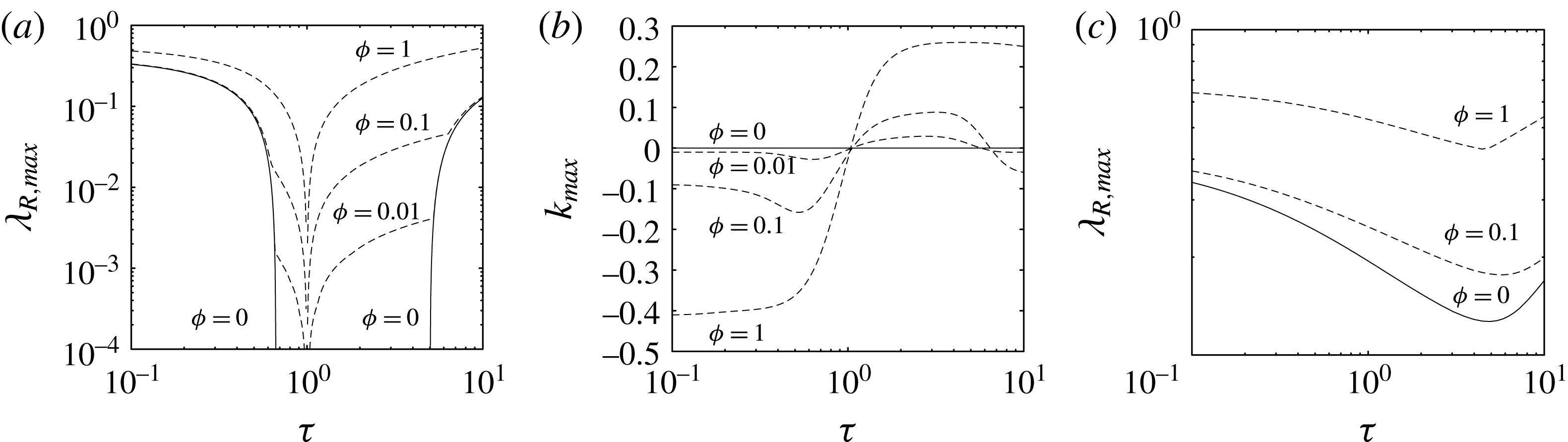
Interesting dynamics is observed when we plot the growth rate as a function of the diffusivity ratio
 $\unicode[STIX]{x1D70F}$
, for select lateral gradient values
 $\unicode[STIX]{x1D719}$
and in the absence of a settling velocity, cf. figure 12. Consistent with earlier findings by other authors, for
 $\unicode[STIX]{x1D70F}<1/R_{\unicode[STIX]{x1D70C}}$
all values of
 $\unicode[STIX]{x1D719}\geqslant 0$
are unstable. For
 $\unicode[STIX]{x1D719}>0$
(but not for
 $\unicode[STIX]{x1D719}=0$
), the interval
 $1/R_{\unicode[STIX]{x1D70C}}<\unicode[STIX]{x1D70F}<1$
becomes destabilized as well. For
 $\unicode[STIX]{x1D70F}=1$
, all values of
 $\unicode[STIX]{x1D719}$
are stable, since neither the double-diffusive nor the settling-driven instability are active. However, for
 $\unicode[STIX]{x1D70F}>1$
, all lateral gradients
 $\unicode[STIX]{x1D719}>0$
are destabilized once again, and for
 $\unicode[STIX]{x1D70F}>5$
we observe the oscillatory ‘diffusive’ mode described earlier for all
 $\unicode[STIX]{x1D719}\geqslant 0$
. Also note that
 $k$
changes its sign as
 $\unicode[STIX]{x1D70F}$
goes from
 ${<}1$
to
 ${>}1$
, indicating that the wavefronts are inclined in opposite directions in these two regimes. Figure 12(c) analyses the influence of lateral gradients on the overall properties of the instability as a function of
 $\unicode[STIX]{x1D70F}$
, in the presence of a settling velocity
 $W_{st}$
. Now all values of
 $\unicode[STIX]{x1D70F}$
, including
 $\unicode[STIX]{x1D70F}=1$
, are destabilized.
 $\unicode[STIX]{x1D70F}=0.01$
,
 $R_{\unicode[STIX]{x1D70C}}=1.5$
,
 $\unicode[STIX]{x1D719}=0.1$
,
 $W_{st}=1$
: maximum real part
 $\unicode[STIX]{x1D706}_{R}$
of the dominant mode growth rate as function of the vertical (
 $k$
) and horizontal (
 $l$
) wavenumbers, for
 $Pr=10^{-3}$
(a),
 $Pr=1$
(b), and
 $Pr=10^{3}$
(c). The dominant mode is marked with ‘
 $\times$
’. The intrusion mode shows little dependence on
 $Pr$
, while the dominant fingering mode is largely independent of
 $Pr$
for
 $Pr\geqslant 1$
.

In the context of certain astrophysical applications a suitably defined Prandtl number can become very small (Medrano et al.
Reference Medrano, Garaud and Stellmach2014), so that it is of interest to examine how the dominant instability mode varies with
 $Pr$
. Figure 13 indicates that the scenarios for
 $Pr=1$
and
 $Pr=10^{3}$
are quite similar with regard to the maximum growth rate, the dominant horizontal and vertical wavenumbers, and the presence of the intrusive mode. For
 $Pr=10^{-3}$
we find that the traditional fingering mode has become less prominent, while the intrusive mode remains relatively unaffected by
 $Pr$
. This suggests that in astrophysical applications the intrusion mode should become increasingly more important as compared to the fingering mode (Medrano et al.
Reference Medrano, Garaud and Stellmach2014).
5 Direct numerical simulation results
In order to analyse the nonlinear evolution of the various instabilities discussed above, we present results from a series of two-dimensional DNS. We solve the governing dimensionless equations by means of a hybrid pseudospectral/compact finite-difference spatial scheme combined with the low-storage Runge–Kutta/Crank–Nicolson time stepping method of Williamson (Reference Williamson1980). The pseudospectral method is used in the horizontal direction, while the vertical direction is discretized using a compact finite-difference method (Lele Reference Lele1992) of up to eighth order. The simulations employ periodic boundary conditions for the perturbation fields in both directions. For a more detailed description of the code and its validation, we refer the reader to Burns & Meiburg (Reference Burns and Meiburg2015). We have also compared DNS growth rates for small perturbations with linear stability results, and we generally found agreement to within a fraction of one per cent. All simulations are initiated with random white noise perturbations to the temperature and sediment concentration fields. Movies of all of the DNS to be discussed below are available in the online supplemental material at https://doi.org/10.1017/jfm.2017.94.
Snapshots of the sediment concentration perturbation field from a two-dimensional simulation for
 $Pr=7$
,
 $\unicode[STIX]{x1D70F}=1$
,
 $R_{\unicode[STIX]{x1D70C}}=1.5$
,
 $\unicode[STIX]{x1D719}=0$
and
 $W_{st}=1$
, with white noise as the initial condition. The domain of size
 $L_{x}=L_{z}=256$
is discretized by
 $N_{x}=N_{z}=1024$
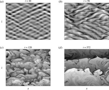
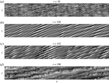
grid points. The instability is purely settling driven, and the wavelengths of the emerging dominant inclined modes are consistent with linear stability results. Eventually, these inclined waves give way to horizontal layers. The time-dependent evolution of the sediment concentration perturbation field in a downward moving reference frame is shown by movie 1 in the supplemental material.

Figure 14 presents DNS results for the sediment concentration perturbation field, for the parameter combination of
 $Pr=7$
,
 $\unicode[STIX]{x1D70F}=1$
,
 $R_{\unicode[STIX]{x1D70C}}=1.5$
,
 $\unicode[STIX]{x1D719}=0$
and
 $W_{st}=1$
. Both species have identical diffusivities, so that double-diffusive effects are absent for this flow, and the instability is driven exclusively by settling. The linear stability results of figure 2 predict dominant instability modes for this case in the form of inclined waves with
 $l_{max}=0.12$
and
 $k_{max}=\pm 0.23$
, corresponding to most amplified horizontal and vertical wavelengths near 52 and 27, respectively. These values are consistent with the DNS observation in figure 14(a) of approximately ten inclined wavefronts over the vertical domain length of
 $L_{z}=256$
, and five to six wavefronts over the horizontal domain length of
 $L_{x}=256$
. Figure 14(b) demonstrates that as a result of the random nature of the initial perturbations, some parts of the flow field become dominated by wavefronts inclined to the right, and other regions by wavefronts inclined to the left. Figure 14(c,d) shows that these inclined wavefronts eventually give way to horizontal layers. The secondary instabilities responsible for the growth of these horizontal layers are analysed in detail in the companion paper by Reali et al. (Reference Reali, Garaud, Alsinan and Meiburg2017).
Snapshots of the sediment concentration perturbation field from a two-dimensional simulation for
 $Pr=7$
,
 $\unicode[STIX]{x1D70F}=0.01$
,
 $R_{\unicode[STIX]{x1D70C}}=150$
,
 $\unicode[STIX]{x1D719}=0$
and
 $W_{st}=5$
, initiated by white noise. The domain of size
 $L_{x}=L_{z}=256$
is discretized by
 $N_{x}=1024$
and
 $N_{z}=4096$
grid points. Since
 $R_{\unicode[STIX]{x1D70C}}>1/\unicode[STIX]{x1D70F}$
, double-diffusive instabilities would not be amplified for
 $W_{st}=0$
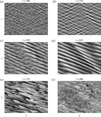
. Inclined waves emerge that dominate the flow during the early stages. Eventually, these inclined waves develop secondary instabilities that cause the flow to break down into small-scale structures. The time-dependent evolution of the sediment concentration perturbation field in a downward moving reference frame is shown by movie 2 in the supplemental material.

Figure 15 displays the nonlinear evolution of the sediment concentration perturbation field for parameter values
 $Pr=7$
,
 $\unicode[STIX]{x1D70F}=0.01$
,
 $R_{\unicode[STIX]{x1D70C}}=150$
,
 $\unicode[STIX]{x1D719}=0$
and
 $W_{st}=5$
. While the diffusivities of the two scalar fields differ by a factor of 100,
 $R_{\unicode[STIX]{x1D70C}}>1/\unicode[STIX]{x1D70F}$
, so that double-diffusive instabilities would not be amplified in the absence of settling, see the linear stability results in figure 8. For
 $W_{st}=5$
, on the other hand, the linear analysis predicts a growing instability in the form of inclined waves with
 $l_{max}=0.07$
and
 $k_{max}=\pm 0.18$
, corresponding to horizontal and vertical wavelengths of approximately 90 and 35, respectively. Again, these values are consistent with the dominant modes observed in the DNS shown in figure 15(a–d). While panels (a) and (b) indicate the emergence of waves inclined in both directions, panels (c) and (d) show that one family of inclined waves eventually dominates of the flow field. Panels (e) and (f) demonstrate that these waves develop secondary instabilities and eventually break down into small-scale structures. By the final time of the simulation, dominant horizontal layers have not evolved.
Snapshots of the sediment concentration perturbation field from a two-dimensional simulation for
 $Pr=7$
,
 $\unicode[STIX]{x1D70F}=5$
,
 $R_{\unicode[STIX]{x1D70C}}=1.5$
,
 $\unicode[STIX]{x1D719}=0.1$
and
 $W_{st}=0$
, initiated by white noise. The domain of size
 $L_{x}=2560$
and
 $L_{z}=256$
is discretized by
 $N_{x}=4096$
and
 $N_{z}=1024$
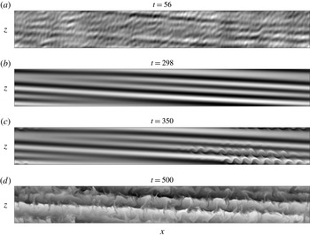
grid points. The flow is initially dominated by an intrusive instability mode. At later times, shear-driven instabilities grow along the interfaces separating neighbouring intrusions, which eventually give rise to small-scale structures superimposed on the intrusion-dominated flow. The time-dependent evolution of the sediment concentration perturbation field can be viewed in movie 3 in the supplemental material.

Figure 16 shows results for a DNS with a horizontal base state gradient, so that it is dominated by intrusive instabilities, but without Stokes settling, for
 $Pr=7$
,
 $\unicode[STIX]{x1D70F}=5$
,
 $R_{\unicode[STIX]{x1D70C}}=1.5$
,
 $\unicode[STIX]{x1D719}=0.1$
and
 $W_{st}=0$
. Note that here the unstably stratified, sedimenting scalar diffuses more rapidly. The linear stability results of figure 12 predict dominant waves inclined to the lower right with
 $l_{max}=0.003$
and
 $k_{max}=0.09$
, corresponding to horizontal and vertical wavelengths of approximately 2000 and 70, respectively. Once again, the linear stability predictions are borne out by the early DNS results of panels (a) and (b). Panel (c) shows the development of shear-driven instabilities along the interfaces separating neighbouring intrusions, while panel (d) indicates the emergence of energetic small-scale structures superimposed on the primarily horizontal intrusions.
Snapshots of the sediment concentration perturbation field from a two-dimensional simulation for
 $Pr=7$
,
 $\unicode[STIX]{x1D70F}=5$
,
 $R_{\unicode[STIX]{x1D70C}}=1.5$
,
 $\unicode[STIX]{x1D719}=0.1$
and
 $W_{st}=0.5$
, initiated by white noise. The domain of size
 $L_{x}=2560$
and
 $L_{z}=256$
is discretized by
 $N_{x}=4096$
and
 $N_{z}=1024$
grid points. The time-dependent evolution of the sediment concentration perturbation field can be viewed in movie 4 in the supplemental material.

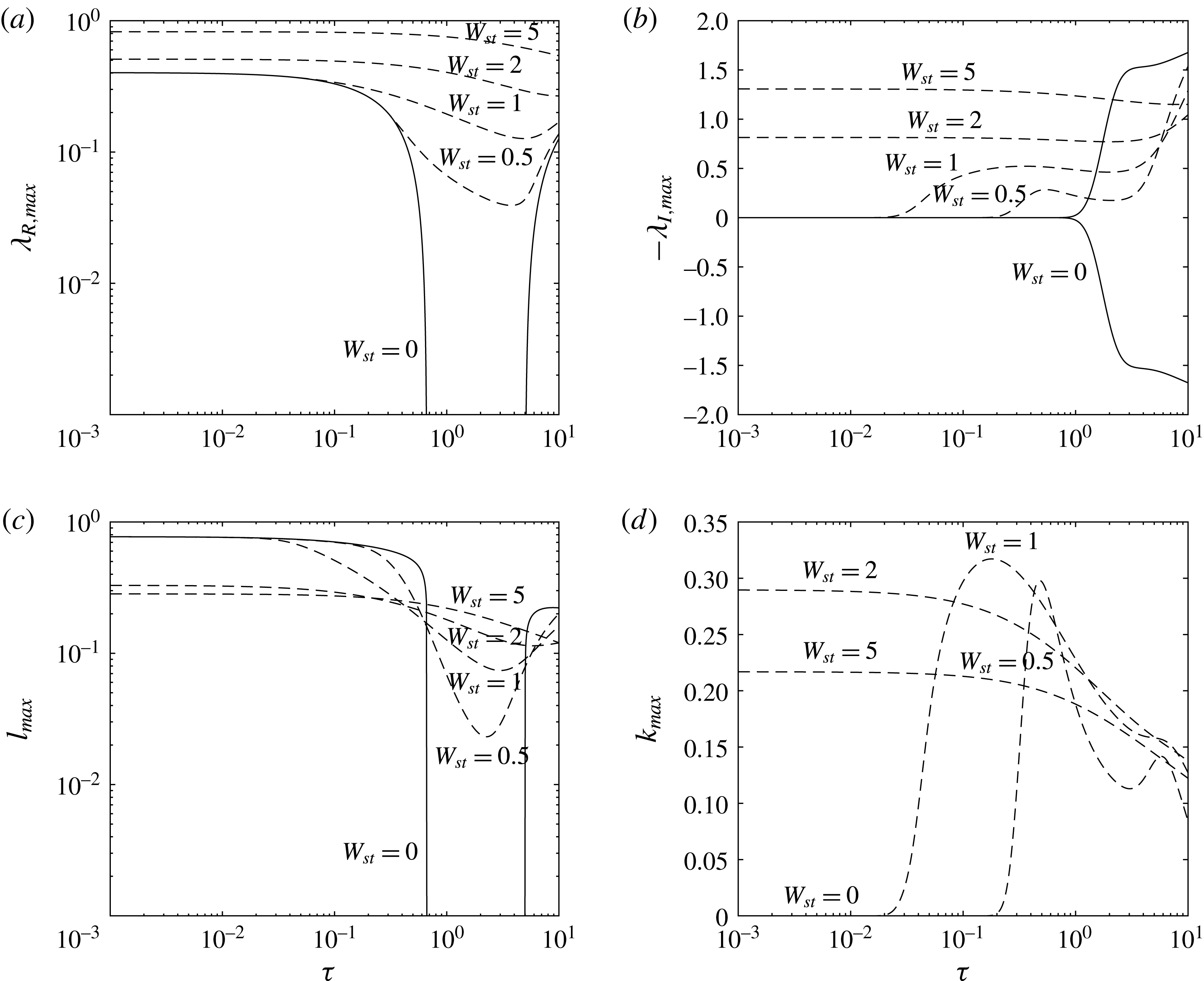
The case shown in figure 17 is identical to that of figure 16, except that it has a settling velocity of 0.5. The linear stability results now predict dominant waves inclined to the lower left with
 $l_{max}=0.03$
and
 $k_{max}=-0.13$
, corresponding to horizontal and vertical wavelengths of approximately 200 and 50, which is consistent with the early DNS results of panels (a) and (b). The comparison of figures 16 and 17 demonstrates that even for flows with horizontal base state gradients, settling can strongly alter the linear and nonlinear flow evolution.
6 Summary
We have presented a linear stability analysis of overall stably stratified fluids whose density depends on two components, where one of these components is unstably stratified and settles. We focus on constant-gradient base states in unbounded domains. The analysis demonstrates that settling generates a phase shift between the perturbation fields of the two scalar components, which gives rise to a novel instability mode driven by settling. This instability mechanism favours the growth of inclined waves, and is active for all density and diffusivity ratios, including for cases in which the two scalars diffuse at identical rates. If the scalar components have unequal diffusivities, the settling-driven instability mode competes with the elevator mode of the classical fingering instability. Detailed linear stability results clarify the balance between the settling-driven and double-diffusive instability modes as a function of the governing dimensionless parameters, and DNS results illustrate the nonlinear competition between the settling mode, the double-diffusive fingering mode and the intrusive mode.
In order to discuss applications of our findings to various geophysical situations, we need to know the expected non-dimensional values of
 $W_{st}$
and
 $\unicode[STIX]{x1D70F}$
for various sediment sizes. These have been computed by Reali et al. (Reference Reali, Garaud, Alsinan and Meiburg2017). They found that for silicate-based particles (clays, silts and sand for instance) of radius
 $r$
, settling in ambient water at room temperature (where
 $d\simeq 0.01$
m, see Radko Reference Radko2013),
 $W_{st}\simeq 0.45(r/10~\unicode[STIX]{x03BC}\text{m})^{2}$
in the Stokes regime. Hence, micron-sized clay particles have
 $W_{st}$
of order
 $10^{-2}$
while fine sand (
 $r\simeq 0.1$
mm) has
 $W_{st}\simeq 10^{2}$
. Assuming that the major contribution to the particle diffusivity comes from hydrodynamic diffusion (Segre et al.
Reference Segre, Liu, Umbanhowar and Weitz2001), they also found that
 $\unicode[STIX]{x1D70F}\simeq rW_{st}/d$
, implying that
 $\unicode[STIX]{x1D70F}\simeq 10^{-4}$
for
 $10~\unicode[STIX]{x03BC}\text{m}$
size particles, increasing rapidly to
 $\unicode[STIX]{x1D70F}\simeq 0.1$
for 0.1 mm-sized particles. The fiducial parameter values we have used in this paper (
 $\unicode[STIX]{x1D70F}=0.01$
and
 $W_{st}$
ranging from 0.5 to 10) would therefore be appropriate for particles a few tens of microns in size (e.g. very fine sand). The above linear stability results indicate that at these
 $W_{st}$
-values the settling instability mode may well dominate over the traditional double-diffusive fingering mode.
To be more precise, let us estimate approximate dimensional length and time scales of the settling-driven instability. Using characteristic length and time scales of
 $d\sim 0.01$
m, and
 $t\sim 10^{3}$
s appropriate for water at ambient temperature, and assuming a moderate value of the density ratio (i.e. not too large) we find that a typical dimensionless wavenumber in the range of 0.1 (e.g. figures 8 and 9) translates into a dimensional instability wavelength of the order of 60 cm. Meanwhile, a dimensionless growth rate of the order of 0.1 to 1 corresponds to a dimensional growth time scale of the order of
 $10^{3}$
s–
 $10^{4}$
s, i.e. on the order of an hour. These ballpark estimates consequently suggest that the settling-driven instability reported here may be relevant in oceans and lakes.
 $R_{\unicode[STIX]{x1D70C}}$
-values in river outflows can range from near unity for extremely high sediment loading to very large values
 $R_{\unicode[STIX]{x1D70C}}\gg 1$
for cases with light sediment loading. The above results imply that even for conditions of
 $R_{\unicode[STIX]{x1D70C}}>1/\unicode[STIX]{x1D70F}$
, where traditional double-diffusive fingering is suppressed, instabilities can evolve as a result of settling.
We hope that the linear stability analysis presented here will serve as the starting point for clarifying several additional features of two-component stratified flows with settling. It will be particularly interesting to quantify the conditions for layer formation, which was observed both here and in the simulations of Reali et al. (Reference Reali, Garaud, Alsinan and Meiburg2017). While the three-dimensional simulations of Reali et al. (Reference Reali, Garaud, Alsinan and Meiburg2017) were limited to
 $Pr=7$
and
 $\unicode[STIX]{x1D70F}=0.3$
, it would be desirable to obtain DNS data for smaller diffusivity ratios such as
 $\unicode[STIX]{x1D70F}=0.01$
, along with the related transport rates, to shed additional light on the layer formation issue.
Acknowledgements
The authors gratefully acknowledge Professors B. Bamieh and M. Wells for helpful discussions, and N. Konopliv for the use of his nonlinear simulation code. Financial support was provided by the Saudi Arabian Oil Company (Saudi Aramco) to A.A., and by NSF grants CBET-1438052 to E.M. and CBET-1437275 to P.G., as well as by grant DN NSWC N00174-16-C-0013 to E.M. Computational resources for this work were made available by the Extreme Science and Engineering Discovery Environment (XSEDE), which is supported by NSF grant TGCTS150053.
Supplementary movies
Supplementary movies are available at https://doi.org/10.1017/jfm.2017.94.