1. Introduction
Various navigation and positioning technologies, using multiple data sources comprehensively and independently of the global navigation satellite system (GNSS), are being developed to address the vulnerability of the GNSS and the resulting service and application limitations. New navigation and positioning technologies at home and abroad have gradually become essential targets of research (Fisher and Racquet, Reference Fisher and Racquet2011; Yang et al., Reference Yang, Liu and Yang2017). Among them, navigation via signals of opportunity (NAVSOP) is a radio navigation and positioning technology with particular emphasis on signals of opportunity (i.e. signals that are intended for purposes other than navigation). NAVSOP can locate the position in an environment where GNSS is not available (Racquet and Martin, Reference Racquet and Martin2008; Li, Reference Li2013; Zuo et al., Reference Yang2019). The proposal of NAVSOP has received considerable attention. Researchers in various countries have actively conducted positioning technology research on opportunity signals, such as A/FM radio, digital television (DTV), mobile communication and Wi-Fi. These techniques mainly rely on ground-based radiation sources and focus on how to extract useful information from various radio signals for positioning and navigation. Martin et al. (Reference Martin, Velotta and Raquet2009) studied the bandwidth of the efficient cooperative time difference of arrival computation for multicarrier signals of opportunity. Merry et al. (Reference Merry, Faragher and Scheding2010) tested and compared several typical random signal positioning effects of the global system for mobile communication (GSM), third generation (3G), digital video broadcast (DVB), digital audio broadcasting (DAB) and so on. Moghtadaiee et al. (Reference Moghtadaiee, Lim and Dempster2010) studied four types of opportunity signal positioning methods (TV, A/FM radio, GSM, and Wi-Fi) from the system-level perspective. Robinson (Reference Robinson2012) studied the topological location of random signals using different measurement methods, including arrival angle, arrival time and arrival time difference. Yang et al. (Reference Yang, Nguyen and Blasch2014) studied the mobile location method of multiple mixed opportunity signals.
Compared with ground-based radiation sources, the satellite-based radiation source has a larger radiation angle, more extensive coverage area of the ground signal, higher elevation angle of the receiving antenna, and less impact by ground clutter and multipath clutter. Meanwhile, the communication and television broadcast satellites in geosynchronous orbit have high signal transmission power and large bandwidth, which can provide high equivalent isotropic radiated power and distance resolution. The use of these satellite-based radiation sources in navigation can be a good supplement and a temporary alternative to the GNSS in environments where the GNSS is unavailable. In 2018, the National Time Service Center (NTSC) proposed a positioning technique using the ubiquitous signals of opportunity of non-cooperative satellites (Gao, Reference Gao2018). This technique positions targets by applying very long baseline interferometry (VLBI) and passive radar detection technologies (Farina and Kuschel, Reference Farina and Kuschel2012; Kuschel et al., Reference Kuschel, Hoffmann and Schroeder2017) to satellite-based navigation via abundant on-orbit communication satellites. It employs communication satellites in a non-cooperative manner using modulated satellite signals, received passively as noise. The technique works by indirectly measuring distances based on the signal correlation.
The positioning technique proposed in this study is different from GNSS because it uses non-ranging signals. GNSS utilises the known characteristic value of the navigation signals to obtain the spread spectrum gain during demodulation, to reduce the influence of interference and noise on useful signals, and to realise a pseudo-range measurement between the receiver and transmitter. Furthermore, considering the configuration cost and convenience for the users, the receiving antenna diameters should be miniaturised as much as possible. Even though it may improve the receiving power and processing performance, and realise high precision measurement of interference, it is difficult to equip the user with the large aperture antenna and complex equipment required for a VLBI observation station (Yang, Reference Yang, Nguyen and Blasch2015). Therefore, it becomes crucial to be able to detect and receive weak communication satellite signals without demodulating the signals in non-cooperative reception, and to achieve a high precision ranging measurement.
2. Principle and model of ranging
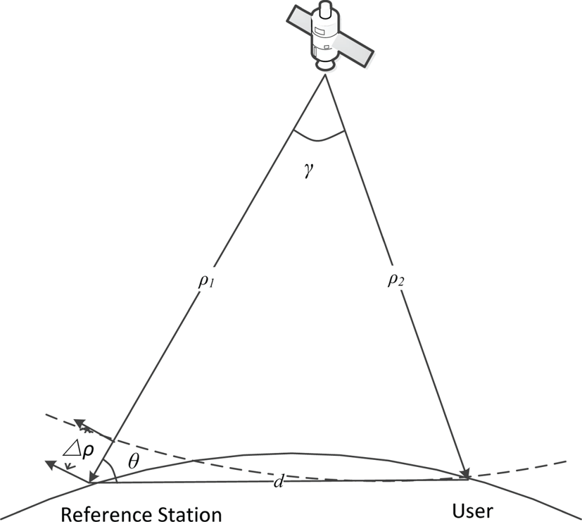
The ranging model of the positioning technique using the ubiquitous signals of non-cooperative communication satellites is similar to the VLBI observation satellite model. Figure 1 illustrates the observation principle using the spherical wave model.
Schematic illustration of the principle of the observation satellite

The leading cause for the time difference in VLBI measurements is the geometric delay, which is determined by the geometric positions of the observed object and the station. The time difference between the satellite signals arriving at two antennas can be expressed as follows (Tornatore and Haas, Reference Tornatore and Haas2009):
 \begin{equation}{\tau _\textrm{g}} = \frac{{({\rho _1} - {\rho _2})}}{c}\end{equation}
where  ${\rho _i} = ||{ {{{\vec{\rho }}_i}} ||} , {\vec{\rho }_i} = \vec{r} - {\vec{R}_i}, {\vec{\rho }_i}$ is the oblique distance vector of the i-th station,
 $\vec{r}$ is the satellite position vector,
 ${\vec{R}_i}$ is the position vector of the i-th station and c is the speed of light.
Each VLBI observation station is provided with an independent atomic frequency standard by a high precision hydrogen atomic clock. The synchronisation is achieved via a two-way satellite time and frequency transfer technique between the VLBI observation stations. The main difference of the proposed technique, with respect to VLBI, is that the clock between the user and the reference station is not synchronised. Furthermore, a clock bias tu exists between the clocks of the user and the reference station. Therefore, the time difference for the proposed positioning technique can be expressed as the following:
 \begin{equation}{\tau _\textrm{g}} = \frac{{({\rho _1} - {\rho _2})}}{{c}} + {t_u}\end{equation}
where the clock bias tu is an unknown quantity. By accurately measuring and estimating the time difference of the arrival of the satellite signal at the reference station and the user, the clock bias tu and the user position can be solved simultaneously.
3. The received signal and time difference estimation method
3.1. The received signal
The measurement principle of the VLBI is applied for the positioning technique proposed here to monitor the satellites in a non-cooperative way without transmitting any signals. Users and reference stations simultaneously receive the downlink signals from multiple satellites. Because of the large scale of equipment and complex configuration of VLBI observation stations, it is challenging for users to configure it. The reference station uses directional antennas pointing in the direction of non-cooperative satellites to obtain a higher gain on the reference signal. The user antenna needs to be as small as possible, and this can be achieved using a single omnidirectional antenna or an array of antennas to receive weak downlink signals from multiple satellites.
The received satellite signals need to be processed by down-conversion. The radio-frequency (RF) signals would be mixed with the local oscillator signal. The VLBI stations are equipped with highly stable hydrogen atomic clocks. In this way, high precision time synchronisation is achieved, and the local oscillator signals are used to minimise the difference among the stations. The received RF signals are down-converted to baseband signals (Deller, Reference Deller2009).
In the proposed positioning technique, the reference station is equipped with a highly stable atomic clock, while the user is equipped only with a crystal oscillator. The frequency and phase of the local oscillator signals cannot be identical, making the mixing output signal unable to maintain the time-delay relationship of the input RF signal, that is, introducing frequency and phase offsets in the process of down-conversion. Moreover, the movement of the satellite emitter relative to the reference station and the non-static user will lead to a differential Doppler (DD) effect, making the interferometry measurement method in VLBI no longer applicable.
According to the above analysis, the received signal of the reference station  ${x_1}(t)$ and the received signal of the user
 ${x_2}(t)$ can be expressed as follows:
 \begin{equation}\left\{ \begin{array}{l} {x_1}(t) = s(t){e^{j({2\pi ({{f_R} - {f_{01}}} )t + {\varphi_1}} )}} + {n_1}(t)\\ {x_2}(t) = As(t - {\tau_g}){e^{j({2\pi ({{f_R} - {f_{02}}} )({t - {\tau_g}} )+ {\varphi_2}} )}} + {n_2}(t) \end{array} \right.,\quad t \in [0,T)\end{equation}
where  $s(t)$ is the signal envelope sent by the emitter, A is the ratio of amplitude attenuation introduced in the transmission of two signals,
 ${f_R}$ is the transmitting frequency of the received signal,
 ${f_{01}}$ and
 ${f_{02}}$ are the local oscillation frequencies of the reference station and the user receiver, respectively;
 ${\varphi _1}, {\varphi _2}$ are the phase values introduced by the local oscillation signals,
 ${\tau _g}$ is the time difference of arrival between the signals,
 ${n_1}(t),{n_2}(t)$ are the observation noises and interferences, and
 $[0,T)$ is the observation interval.
By taking the signals received by the reference station as a reference, the signal model can be simplified. Thus, Equation (3) can be expressed as:
 \begin{equation}\left\{ \begin{array}{l} {x_1}(t) = s(t){e^{j2\pi {f_{_c}}t}} + {n_1}(t)\\ {x_2}(t) = As(t - {\tau_g}){e^{j({2\pi ({{f_c} + \Delta f} )({t - {\tau_g}} )+ \varphi } )}} + {n_2}(t) \end{array} \right.,\quad t \in [0,T)\end{equation}
where  ${f_c}$ is the intermediate frequency of the carrier-wave (IF) after the down-conversion of the reference station,
 $\Delta f$ is the frequency difference of the local oscillator signals between the receiver and the reference station.
 $\varphi$ is the initial phase difference of the local oscillator signal between the receiver and the reference station, that is,
 $\varphi = {\varphi _2} - {\varphi _1}$. Generally, the signal
 $s(t)$ and noises
 ${n_1}(t)$ and
 ${n_2}(t)$ are uncorrelated with each other. According to the conventional cross-correlation method (Gardner and Chen, Reference Gardner and Chen1992), it can be expressed as the following:
 \begin{equation}\begin{aligned} {R_{{x_1}{x_2}}}(\tau )& =\dfrac{1}{T}\int_0^T {{x_1}(t)x_2^\ast (t + \tau )dt} \\ & =\dfrac{1}{T} \cdot A\int_0^T {s(t){e^{j({2\pi {f_c}t} )}}{s^\ast }(t - {\tau _g} + \tau ){e^{ - j({2\pi ({{f_c} + \Delta f} )(t - {\tau_g} + \tau ) + \varphi } )}}dt} \\ & ={e^{j2\pi ({{f_c} + \Delta f} )({{\tau_g} - \tau } )+ j\varphi }} \cdot \dfrac{1}{T} \cdot A\int_0^T {s(t){s^\ast }(t - {\tau _g} + \tau ){e^{ - j2\pi \Delta \textit{ft}}}dt} \end{aligned}\end{equation}
According to Schwartz inequality, it can be expressed as follows:
 \begin{equation}\begin{aligned} |{{R_{{x_1}{x_2}}}(\tau )} |& = \left|{{e^{j2\pi \cdot ({{f_c} + \Delta f} )\cdot ({{\tau_g} - \tau } )+ j\varphi }} \cdot \dfrac{A}{T} \cdot \int_0^T {s(t){s^\ast }(t - {\tau_g} + \tau ){e^{ - j2\pi \Delta \textit{ft}}}dt} } \right|\\ & = \left|{\dfrac{A}{T}\int_0^T {s(t){s^\ast }(t - {\tau_g} + \tau ){e^{ - j2\pi \Delta ft}}dt} } \right|\\ & \le A \cdot |{{R_{ss}}(\tau - {\tau_g})} |\cdot \left|{\dfrac{{{e^{ - j2\pi \Delta fT}} - 1}}{{ - j2\pi \Delta fT}}} \right|\end{aligned}\end{equation}
where  ${R_{ss}}(\tau - {\tau _g}) = \int_0^T {s(t){s^\ast }(t - {\tau _g} + \tau )dt}$ is the correlation function of the useful signal
 $s(t)$. Assuming
 $\theta ={-} 2\pi \Delta fT$, Equation (6) can be expressed in the following manner:
 \begin{equation}|{{R_{{x_1}{x_2}}}(\tau )} |\le |{{R_{ss}}(\tau - {\tau_g})} |\cdot \left|{\frac{{({e^{j\theta }} - 1)}}{{j\theta }}} \right|\end{equation}
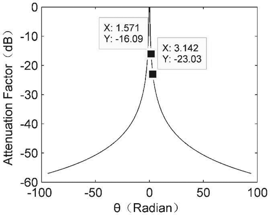
The attenuation factor  $|{({e^{j\theta }} - 1)/j\theta } |$ varies with the phase difference
 $\theta$ as shown in Figure 2.
Attenuation factor varies with the phase difference

As shown in Figure 2, when the frequency difference is zero, the attenuation factor is zero and the correlation peak is multiplied by the constant 1, which is the case in VLBI. Moreover, when the accumulation of the frequency difference with time provides the phase difference, the attenuation in the correlation peak increases. Furthermore, when the phase difference reaches  ${\pm} (\pi /2)$, the attenuation can reach 16 dB, and when the phase difference reaches
 ${\pm} \pi$, the attenuation can reach 23 dB. Therefore, the frequency difference can restrain the peak value of the cross-correlation function. For the initial phase difference (φ) in the derivation of Equation (4), the output amplitude correlation will not be affected by the introduced complex signal correlation.
3.2 Analysis of frequency difference
Considering the analysis presented in Section 3.1, the frequency difference introduced in the measurement will affect the time difference estimation. In this section, the possible frequency differences are analysed, the range is estimated, and its impact on the time difference estimation is evaluated.
3.2.1 Phase and frequency difference introduced by the mixing local oscillator
In the proposed positioning technique, due to the introduction of a clock difference variable, the time difference measurement performance required is at the nanosecond level. While the hydrogen atomic clock is a requirement for a VLBI observation station, the requirement of time keeping performance of a reference station is reduced. Therefore, a rubidium or caesium atomic clock can also meet the requirements of time synchronisation of the system.
The clock at the reference station is the time measurement reference. The frequency of the reference station is generated based on atomic clocks (rubidium, caesium and hydrogen atomic clocks) with high accuracy and stability. For cost effectiveness, the users usually employ a quartz crystal oscillator as a measure of time and frequency. The frequency deviation is caused by the difference between the local oscillator signals of the reference station and the user. The frequency accuracy of the atomic clock and the crystal oscillator are  ${F_1},{F_2}$, respectively.
 ${f_0}$ is the standard frequency and
 $\Delta {f_1},\Delta {f_2}$ are the differences between the actual frequencies and the standard frequency. Subsequently, according to the accuracy definition, the following equation can be derived:
 \begin{equation}\left\{ \begin{array}{l} {F_1} = \dfrac{{\Delta {f_1}}}{{{f_0}}}\\ {F_2} = \dfrac{{\Delta {f_2}}}{{{f_0}}} \end{array} \right.\end{equation}
The frequency difference between two signals mixing with the local oscillator is as follows:
 \begin{equation}\begin{aligned} \Delta f & = \Delta {f_2} - \Delta {f_1}\\ & = {F_2}({f_R} - {f_c}) - {F_1}({f_R} - {f_c}),\\ & = ({{F_2} - {F_1}} )\cdot ({f_R} - {f_c}) \end{aligned}\end{equation}
where  ${f_R}$ is the transmitting frequency of the received signal and
 ${f_c}$ is IF after down-conversion.
Assuming that the range of  ${f_R}$ is 3,400–4,200 MHz, which is the common downlink frequency of C-band,
 ${f_c}$ is 70 MHz. The frequency accuracy of the hydrogen atomic clock is generally 10−12, the frequency accuracy of the commercial caesium clock is generally 1⋅5 × 10−12 –3 × 10⁻¹¹ (Qi, Reference Qi2006), and the frequency accuracy of a quartz crystal is generally 2⋅5 × 10−7–2 × 10⁻⁴ (Xie, Reference Xie2009). Subsequently, according to Equation (9), the frequency difference range introduced by mixing in this frequency band is approximately 832–826 kHz. When the correlation integration time is at the millisecond range, the frequency difference has a great attenuation effect on the time difference measurement.
To improve the related execution efficiency, the synchronisation accuracy between the user and the reference station is in the millisecond range. This range can fulfil the technical requirements of the time difference measurements for the proposed positioning technique. In case of GNSS denial, the long-wave time service system, a ground-based, low-frequency, high-power and independent timing system, can cover approximately 1,000 km by ground wave signals and provide timely service with a precision of several microseconds (μs). The accuracy of the frequency calibration can reach 10−12 (Li, Reference Li2015). Therefore, the user can be equipped with a long-wave timing receiver to perform a coarse synchronisation with the reference station. The crystal oscillator of the user receiver is disciplined by using a long-wave timing signal to improve the accuracy of the local oscillation frequency. Subsequently, the reception of two signals maintains proper consistency. When the frequency accuracy of the user receiver is better than 10−10 s, the frequency difference introduced by the local oscillator is of several Hz with a small accumulated phase difference, for the integration time of several milliseconds. In this case, the influence on time difference measurement can be neglected.
3.2.2 The DD effect
When the relative motion of the non-cooperative radiation source to the reference station and the user receiver cannot be ignored, the Doppler frequency shift of the two signals received separately by the reference station and the user receiver is different; this causes a frequency difference.
The satellite constellation for the positioning technique in this study mainly consisted of geostationary Earth orbit (GEO) and inclined geosynchronous orbit (IGSO) satellites (Gao, Reference Gao2018). GEO satellites are static in relation to a static target located on the ground, and the Doppler frequency shift is approximately zero. The maximum velocity of the vehicle target on the ground is approximately 30 m/s, wherein the Doppler frequency shift of the target to GEO satellites is calculated within several Hz in the C-band, and the accumulated phase difference is small, considering the integration time of several milliseconds. Therefore, the influence of the relative motion of the moving ground target on the time difference measurement can be neglected. For high-speed moving targets on other moving carriers, when the velocity is over 100 m/s, DD may reach several hundred Hz to several thousand Hz, affecting the time difference estimation.
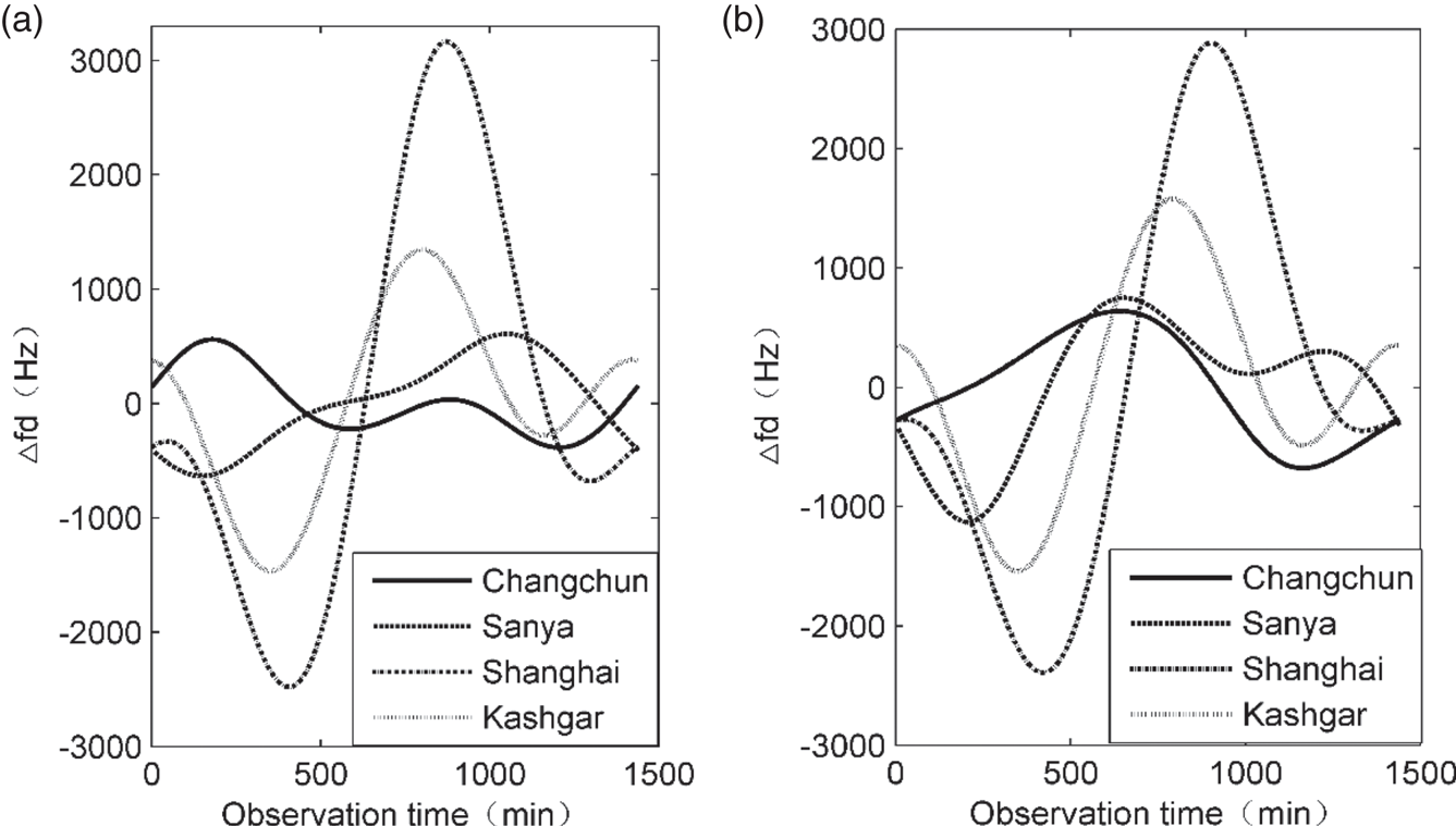
Fixed reference stations and users on the ground are no longer static in relation to the IGSO satellite emitters, which makes it necessary to consider DD. Thus, it is assumed that the reference station and the user are both static, and the motion of the IGSO satellite is the only source of DD. The variation of DD at different user positions is estimated by taking two BeiDou IGSO satellites, namely, IGSO1 (118 °E) and IGSO4 (95 °E), respectively, as radiation sources and the site of the Xi'an Satellite Control Centre as a reference station. Figure 3 shows the calculation of the DD at four user positions (Shanghai, Kashgar, Sanya, Changchun) of a B1 frequency signal from UTC 12:00:00 on 22 October to 12:00:00 on 23 October 2017.
DD of different IGSO satellites at different user positions: (a) IGSO1, (b) IGSO4

As shown in Figure 3, the DD introduced by the motion of the IGSO satellites varies greatly, reaching several kHz, and the corresponding attenuation to the correlation peak for accumulation with the time of several milliseconds can reach over 30 dB. Therefore, the influence of the DD on the time difference measurement cannot be neglected.
3.3 Time difference estimation method and simulation verification
Based on the above analysis, the frequency difference between the two received signals is unavoidable in practice, which is mainly determined by the received signals, the motion characteristics of the satellite emitter and the motion state of the user. The phase difference accumulated in the integration time of several milliseconds will affect the time difference estimation performance due to a frequency difference of dozens of Hz. Therefore, the introduction of a joint time–frequency estimation method based on the ambiguity function (Dandawatr and Giannakis, Reference Dandawatr and Giannakis1993; Fowler and Hu, Reference Fowler and Hu2008; Kim et al., Reference Kim, Park, Kim, Park, Park and Shin2018) in passive detection technology can effectively solve the limitations of the correlation time-delay estimation method in VLBI interferometry. The cross-ambiguity function definition of the reference station signal  ${x_1}(t)$ and user receiver signal
 ${x_2}(t)$ can be expressed as follows:
 \begin{equation}{\chi _{{x_1}{x_2}}}(\tau ,f) = \int_{\tau = 0}^{{T_0}} {{x_1}(t) \cdot {x_2}^\ast (t + \tau ) \cdot } {e^{j2\pi ft}}dt\end{equation}
From the signal model given in Section 3.1, the following equation can be derived:
 \begin{equation}\begin{aligned} {\chi _{{x_1}{x_2}}}(\tau ,f) & = \dfrac{1}{T}A \cdot {e^{j2\pi ({{f_c} + \Delta f} )(\tau - {\tau _g}) + j\varphi }} \cdot \int_0^T {s(t){s^\ast }(t + \tau - {\tau _g})} {e^{j2\pi (f - \Delta f)t}}dt\\ & = A{e^{j2\pi ({{f_c} + \Delta f} )(\tau - {\tau _g}) + j\varphi }} \cdot {\chi _{ss}}(\tau - {\tau _g},f - \Delta f) \end{aligned}\end{equation}
where  ${\chi _{ss}}(\tau ,f) = (1/T)\int_0^T {s(t){s^\ast }(t + \tau )} {e^{j2\pi ft}}dt.$
According to Schwartz inequality and trigonometric inequality,
 \begin{equation}\begin{aligned} \left|{\int_0^T {s(t){s^\ast }(t + \tau )} {e^{j2\pi ft}}dt} \right|&\le \int_0^T {|{s(t){s^\ast }(t + \tau )} |} dt = {\int_0^T {|{{s^2}(t)} |} ^{{1 / 2}}} \cdot {|{{s^2}(t + \tau )} |^{{1 / 2}}}dt\\ & \le {\left( {\int_0^T {|{s{{(t)}^2}} |} dt} \right)^{{1 / 2}}} \cdot {\left( {\int_0^T {|{{s^2}(t + \tau )} |} dt} \right)^{{1 / 2}}} = \int_0^T {|{s{{(t)}^2}} |} dt \end{aligned}\end{equation}
Therefore, the following inequality can be derived:
 \begin{equation}{\chi _{ss}}(\tau ,f) \le {\chi _{ss}}(0,0)\end{equation}
Subsequently, the following inequality is derived:
 \begin{equation}|{{\chi_{{x_1}{x_2}}}(\tau ,f)} |\le |{{\chi_{{x_1}{x_2}}}({\tau_g},\Delta f)} |\end{equation}
That leads to the estimation of the time difference  ${\tau _g}$ and the frequency difference
 $\Delta f$ corresponding to the maximum value of the function
 $|{{\chi_{{x_1}{x_2}}}(\tau ,f)} |$.
 \begin{equation}\left( {\mathop {{\tau_g}}\limits^ \wedge ,\mathop {\Delta f}\limits^ \wedge } \right) = \arg \left\{ {\mathop {\max }\limits_{\tau ,f} [{|{{\chi_{{x_1}{x_2}}}(\tau ,f)} |} ]} \right\}\end{equation}
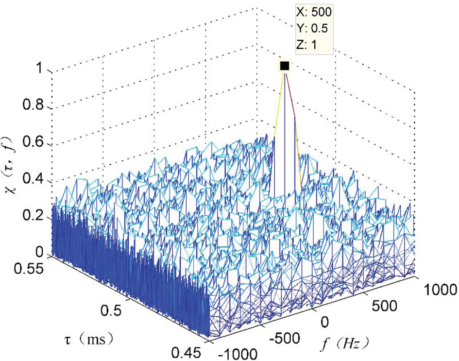
The signals transmitted by communication or broadcasting satellites are random aperiodic signals, occupying a wide frequency range and containing a variety of modulation modes. For example, the signals of multiple channels are mixed in the digital satellite television, each channel including the amplitude modulation (AM) signal of the television image and the frequency modulation (FM) signal of the accompanying sound (Merry et al., Reference Merry, Faragher and Scheding2010). These signals are approximated as random signals after source and channel coding. The satellite communication channel is a typical band-limited channel; therefore, the continuous band-limited white noise signal was simulated as the source signal with unrelated white Gaussian noise. The signal bandwidth is 30 MHz, the centre frequency is 70 MHz, the signal-to-noise ratio (SNR) of the signal received by the reference station is 10 dB, and the SNR of the signal received by the user is –38 dB. The frequency difference between the two signals is 500 Hz, and the time difference is 0⋅5 ms. As shown in Figure 4, even though the SNR is low, the cross-ambiguity function is still in the form of a graph pin, and the correlation peak appears everywhere, allowing the estimation and measurement of the time difference to be performed.
The cross-ambiguity function of communication satellite signals

As shown in Figure 4, although the signals received from non-cooperative communications or broadcasting satellites are unknown and random, the different arrival time and distance from the satellite to the user and the reference station can be estimated using the excellent correlation characteristics of the random signals.
4. Test verification of time difference measurement
4.1. Construction of the test platform
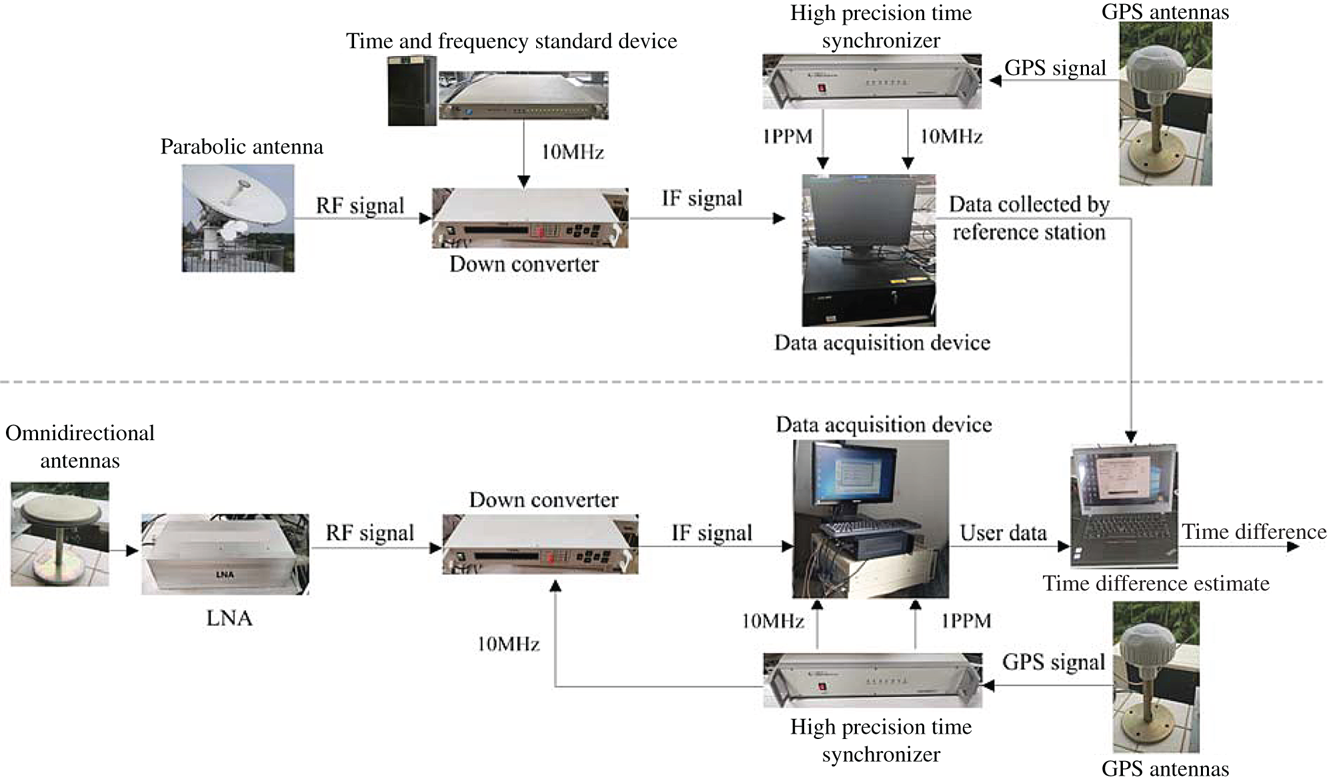
To verify the feasibility and performance of the proposed time difference measurement method based on non-cooperative communication satellite signals, we generated a test platform for the time difference measurement. The test platform is mainly composed of a C-band receiving antenna, a down-converter, a data acquisition and storage device, a hydrogen clock, a high precision time synchroniser and the time difference estimation terminal. Figure 5 shows a block diagram of the composition of the test platform.
Block diagram of time difference measurement test platform

The reference station is equipped with a C-band parabolic antenna with an aperture of 3⋅7 m, pointing in the direction of the radiationof the non-cooperative satellite to obtain a reference signal with a higher gain. The RF signal received by the antenna needs to be processed by a down-converter. The input signal bandwidth is 36 MHz, the output frequency is 70 MHz, the gain is 45 dB, and the noise coefficient is less than 12 dB. The external frequency standard of the down-converter is provided by a hydrogen atomic clock having a frequency accuracy of 3 × 10⁻¹³. The user receiver is equipped with C-band omnidirectional antennas. The weak RF signal received by the antenna is amplified with an appropriate gain power, and subsequently the RF signal is converted to an IF signal. The external frequency standard for the user receiver down-converter is provided by a high precision time synchroniser having a frequency calibration accuracy of 3 × 10⁻¹². According to the theoretical calculation presented in Section 3.2, the frequency difference introduced by the local oscillator can be neglected. The data acquisition device converts the IF analogue signal to an IF digital signal for sampling and storing the data label timestamp information.
In practice, the reference station acquisition device should provide the standard 1 ppm and 10 MHz according to the high precision atomic clock. The time and frequency standard devices should be traceable to the standard coordinated universal time UTC (NTSC). The user should be provided with the standard 1 ppm and 10 MHz by the long-wave timing receiver to achieve a coarse synchronisation with the reference station and ensure regular operation in cases of GNSS denial. This test focuses on assessing the performance and the accuracy of the time difference measurement. Thus, the high precision time synchroniser based on the GPS signal replaces the long-wave timing receiver, reducing the influence of clock biases between the reference station and user on the time difference measurement.
4.2. Time difference measurement test
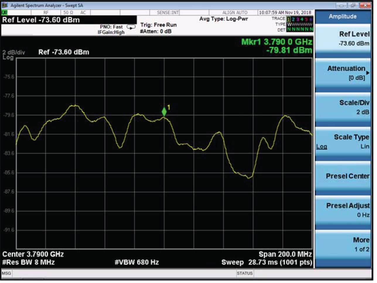
An unknown communication signal with a frequency of 3,790 MHz was observed by the test platform from 9:36 to 15:36 (Beijing Time) on 16 July 2018. Firstly, the directional antenna of the reference station was aligned to the radiation direction of the non-cooperative satellite, namely Apstar 7, and it received the satellite signal. The spectrum of the signal was observed using the analyser. Figure 6 shows the spectrum of the communication satellite signal.
Spectrum of the signal from a communication satellite with a frequency of 3,790 MHz observed by the test platform

Figure 6 shows a broadband signal with a bandwidth of 27 MHz at the frequency point of 3790 MHz. The joint estimation of the time–frequency difference based on the ambiguity function was conducted for the collected wideband signal.
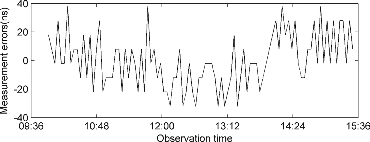
The position of the reference station was calibrated in advance to test the accuracy of the time difference measurement, and the user position information was acquired by the GPS precise point positioning (PPP) (24-hour measurement data, positioning accuracy can reach the centimetre level). The observation satellite ephemeris was provided by the determining system's transponding satellite orbit, and the theoretical time difference of the satellite signals arriving at the reference stations and users were calculated. The test measurements were compared with the results of the theoretical model, and the time difference measurement errors were obtained, as shown in Figure 7.
Error in time difference of the communication signal in the test

The time difference measurement accuracy is 18⋅4 ns by the statistical calculation of the measurement errors presented in Figure 7, corresponding with the ranging accuracy, which is better than 6 m. The output of the spectrometer in Figure 6 shows that the signal power received by the reference station is −81⋅29 dB, and the SNR is approximately 0 dB. It is estimated that the SNR of the signal received by the user is nearly −28 dB. According to the formula of the Cramer–Rao bound for the accuracy of time difference estimates (Stein, Reference Stein1981), the limit of time difference measurement accuracy is 0⋅9 ns.
According to the test results, the measured accuracy differs significantly from the theoretical limit value with 0⋅9 ns time difference and measurement accuracy of 18⋅4 ns. The reasons are detailed below.
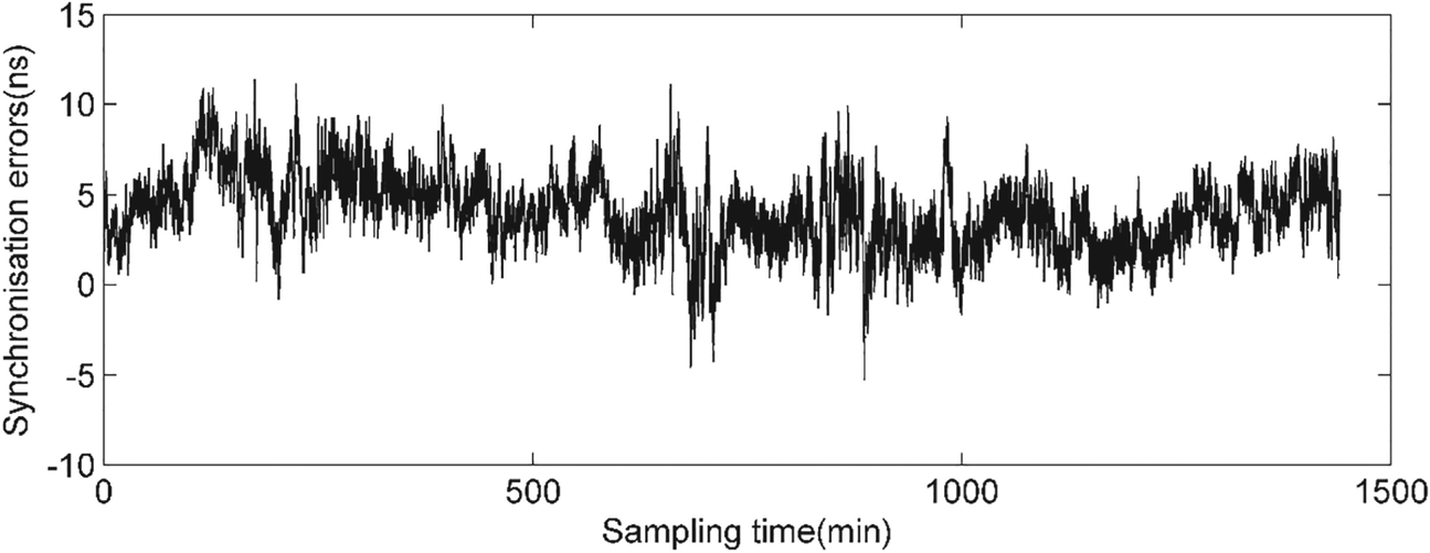
Firstly, the data acquisition devices of the reference station and the users employ different time pulse signals provided by the high precision time synchronisers based on the GPS signal to trigger. Therefore, the synchronisation accuracy of the high precision time synchronisers will affect the performance of the time difference measurement. The error introduced by the synchronisers was assessed by measuring the time difference of 1 ppm output between two synchronisers. Figure 8 shows the synchronisation error between the two synchronisers for 24 hours. It shows that the synchronisation error fluctuates between –6 and 12 ns, and the root mean square (RMS) is approximately 4⋅5 ns. Secondly, except for the synchronisation error, the resolution of the time difference measurement platform is only 10 ns.
Synchronisation error between time synchronisers obtained in 24 h

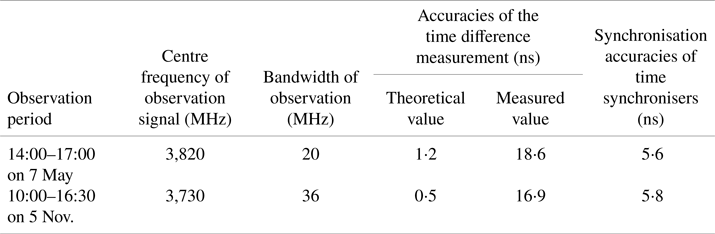
At 14:00–17:00 on 7 May 2018 and 10:00–16:30 on 5 November 2018 (Beijing time), the test platform was used to observe Apstar 7, and the time difference measurement tests were conducted with a baseline length of approximately 40 km. The baseline length between the base station and the user affects the cancellation effect of the signal propagation path delay error. The satellite ephemeris error, ionospheric delay and tropospheric delay have spatial and temporal correlations. When the baseline is short, the satellite ephemeris error, ionospheric delay and tropospheric delay can be effectively eliminated. When the baseline is long, the ionospheric delay and tropospheric delay can be corrected using the model, which is similar to the error cancellation of single difference pseudo-range positioning in a GNSS system. The test results are presented in Table 1.
Results of the time difference measurement tests

From the above test results, the feasibility of the time difference measurement technology based on non-cooperative weak satellite signals has been verified, and the performance of the measurement has been validated adequately. The measured results are related to the observed signal bandwidth, SNRs of received signals, synchronisation accuracy and propagation path error correction. However, considering the theoretical calculation results, it is possible to further improve the time difference measurement technology by increasing the signal sampling frequency, correcting the propagation path delay and calibrating the receiver.
5. Conclusions
A high precision ranging technology for non-cooperative observation communication satellites has been developed. The proposed approach was achieved by employing the ranging model of VLBI observation satellites and combining the joint estimation algorithm of time–frequency difference in passive radar detection technology. A test platform for time difference measurement was built to observe the GEO communication satellite and collect an unknown communication signal for its measurement and estimation. The ranging technology has an accuracy of better than 6 m. Therefore, the feasibility of this ranging technology is adequately validated. However, there are still many technical challenges to building a safe and reliable positioning system. At present, the research and verification of this positioning method are still in the early stages. The receiving conditions of non-cooperative satellite signals are relatively complex; therefore, the analysis of ranging technology needs to expand further, and a variety of testing and verification methods will be a key point of the follow-up process. For example, the baseline length between the reference station and the user will cause the change in the signal propagation path and delay error, thus affecting the ranging accuracy. Different motion states have different requirements for the real-time performance of the time difference measurement. For highly dynamic users, the efficient real-time data interaction between the users and reference stations is a critical problem. It can form different observation schemes according to the diversity of constellations, leading to the optimisation of time difference measurement processing and estimation.
Acknowledgements
We would like to thank Editage [www.editage.cn] for English language editing.
Funding statement
This research was funded by Defense Innovation Funding (grant number 17-H863-01-ZT00100605).