2.1. Free-stream conditions and geometry

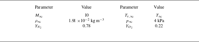
The free-stream conditions used here are the same as Knisely & Zhong (Reference Knisely and Zhong2019b , Reference Knisely and Zhongc , Reference Knisely and Zhong2020) and are summarised in table 1. The free-stream stagnation enthalpy is $h_{0,\infty } \approx$ 9.17 MJ kg^–1 and the unit Reynolds number is $Re_1 \approx$ 1.72 $\times$ 10 $^{6}$ m $^{-1}$ . These conditions are similar to those found in high-enthalpy shock tunnels. The geometry is a circular cone with a nose radius of 1 mm and a half-angle of 5 $^{\circ }$ at zero angle of attack.

Table 1.

Free-stream conditions for present study. The temperatures are not specified a priori, but are computed from the remaining quantities.

2.2. Cases

For the above flow configuration, direct numerical simulation (DNS) is performed for two cases using different gas models. The first case (hereafter referred to as the TCNE case) uses a TCNE gas model that includes finite-rate chemistry based on a five-species air model, as well as a two-temperature model for the translation–rotation and vibration temperatures. The governing equations are given in § 3. The wall is assumed to be isothermal and in thermal equilibrium with $T_w$ = $T_{v}$ = 600 K and non-catalytic for the species mass fractions.

The second case (hereafter referred to as the frozen case) considers a thermochemically frozen gas in which the species mass fractions and vibration temperature remain at their free-stream values everywhere in the flow field. This was implemented in the DNS by neglecting the chemical production/depletion term ( $\omega _s$ ) and the translation–vibration energy transfer term ( $Q_{T-V,s}$ ), and by setting the species mass fractions and vibration temperature at the wall to their free-stream values. The wall is assumed to be isothermal for the translation–rotation temperature at $T_w$ = 600 K.

Note that, because $\omega _s$ and $Q_{T-V,s}$ are neglected in the frozen case, the vibration energy equation can be subtracted out from the total energy equation such that the vibration temperature no longer appears as a variable in the equation set. Hence, the vibration temperature becomes a passive variable and is ultimately irrelevant to the results. Because of this, and because the species mass fractions are also uniform in this case, we would obtain functionally the same results if we instead considered a CPG model, where the vibrational energy is neglected entirely and species mass fractions are fixed.

2.3. Wall temperature considerations

It should be noted that the wall temperature used in this study is higher than what is typically observed in high-enthalpy wind tunnels. In reality, because of short test durations, the wall temperature remains close to the ambient temperature (usually around 300 K) for the entire test. Such a cold wall is difficult to simulate numerically because of the high temperature (and density) gradients. However, even with the present wall temperature of 600 K, the wall is considered to be cold, with a nominal wall-to-edge temperature ratio of $T_w/T_e \approx$ 0.24 on the frustum. As such, the results of the present study are expected to at least be qualitatively consistent with experimental results in terms of boundary-layer receptivity.

2.4. Direct numerical simulation grid and grid convergence

The DNS is performed up to $s$ = 1.25 m, where $s$ is the arclength measured along the surface starting from the stagnation point. The wall-normal grid uses 513 grid points. The streamwise grid uses at least 10 grid points per millimetre up to $s \approx$ 0.6 m and approximately 5 grid points per millimetre between $s \approx$ 0.6 and $s$ = 1.25 m. Since the flow field is axisymmetric, the azimuthal direction uses only 4 grid points.

The grid convergence is assessed using the grid convergence index (GCI) described by Roache (Reference Roache2009), which is essentially a measure of the uncertainty arising from the discretisation error. The GCI is evaluated in terms of the amplitude of mode $F_1$ (the unstable mode) at the branch I and II neutral points (the point at which the unstable mode goes becomes unstable and stable again, respectively). Errors beyond the branch II neutral point are not relevant to this study. The branch I and II neutral points are taken to be those predicted by the linear parabolised stability equations (LPSE) except for the wall-normal grid convergence analysis, where the linear stability theory (LST) ones are used instead. The neutral points do not vary substantially between the two stability frameworks. The grid convergence analysis is performed for the TCNE case only, although the results should apply for the frozen case as well because of the similarities in the flow fields and grid stretching parameters used. For this analysis, we consider a fixed frequency of $f$ = 600 kHz.

The GCI for the wall-normal discretisation is estimated by performing an LST analysis using the mean flow profiles from the present DNS (using 513 points in the wall-normal direction), and comparing the results with those obtained using the mean flow profiles from two separate DNSs using 385 and 769 points in the wall-normal direction. The resulting comparison is shown in figure 1(a). The error from the LST discretisation itself is least two orders of magnitude smaller than the error from the underlying DNS base flow and does not affect the GCI estimate. The LST computations follow the streamwise evolution of the amplitude of mode $F_1$ relative to a starting location of $s$ = 0.01 m. This amplitude is computed by integrating the growth rate. The accumulated error upstream of the starting location is assumed to be negligible. Following Roache (Reference Roache2009), the GCI is estimated by computing an empirical order of accuracy $p_{emp}$ (which in this case is less than $p$ = 5, the theoretical order of accuracy), performing Richardson extrapolation using $p_{emp}$ , then multiplying the resulting error by a factor of safety of 1.25. In doing so, the wall-normal GCI in terms of the branch I and II amplitudes are 1.79 $\,\%$ and 3.29 $\,\%$ , respectively.

Figure 1.

(a) Comparison of LST-derived second-mode amplification ratio relative to $s$ = 0.01 m between the present DNS grid (with 513 points) and finer and coarser DNS grids (with 769 and 385 points, respectively) in the wall-normal direction. (b) Comparison of wall pressure perturbation amplitude with free-stream slow acoustic waves between the present DNS grid and a coarser DNS grid with half the number of points in the streamwise direction, starting from $s$ = 0.01 m.

The GCI for the streamwise discretisation is computed by comparing unsteady DNS results (with imposed free-stream slow acoustic waves) with another DNS with a coarser grid, with roughly half the number of streamwise points between $s \approx$ 0.01 and $s$ = 1.25 m. Figure 1(b) compares the wall pressure amplitude between the two grids. Errors accumulated upstream of $s \approx$ 0.01 m are assumed to be negligible. Note that the boundary-layer disturbance is nominally multimodal, containing not only mode $F_1$ , but other types of waves as well. However, the boundary-layer disturbance at the branch II neutral point is dominated by mode $F_1$ . Hence, the disturbance amplitude at this point is essentially the amplitude of mode $F_1$ . The amplitude of mode $F_1$ at the branch I neutral point is estimated through a backtracking method described later in this paper. The GCI is estimated here by performing Richardson extrapolation with $p$ = 5 (the theoretical order of accuracy) and multiplying the resulting error by a factor of safety of 3. This more conservative factor of safety is recommended by Roache (Reference Roache2009) since the empirical order of accuracy is not known in this case (only two grids are considered). The streamwise GCI in terms of both the branch I and II amplitudes is approximately 0.72 $\,\%$ . The streamwise GCI is the same between the two locations due to the nature of the backtracking method mentioned earlier.

The GCI for the temporal discretisation is estimated by running a 1-D inviscid perfect gas simulation with a slightly larger time step but the same Runge–Kutta method as the last subdomain in the full DNS (spanning from $s \approx$ 0.6 to $s$ = 1.25 m). The mean flow conditions roughly approximate those at the boundary-layer edge at $s$ = 1 m. The simulation is initiated with slow acoustic waves at the inlet. The dissipation rate per wavelength associated with the temporal discretisation (which is primarily dissipative) is estimated. Extrapolating these results to the distance of the branch I and II neutral points, the temporal GCIs in terms of the branch I and II neutral points are 0.045 $\,\%$ and 0.069 $\,\%$ , respectively.

The combined GCIs in terms of the amplitude at the branch I and II neutral points are approximately 2.56 $\,\%$ and 4.08 $\,\%$ , respectively. The GCI for the branch I amplitude in particular may appear to be excessive when considering the branch I receptivity coefficients (see figure 22), where the differences between the TCNE and frozen cases are of the same order of magnitude as the GCI. However, because the two cases have similar overall flow fields, they have similar grid resolution requirements, and similar discretisation errors. This means the comparisons of results between the TCNE and frozen cases will essentially be unchanged regardless of the number of points used in the grid, as long as the same grid stretching parameters are used. This was verified by comparing low-resolution steady DNS results between the two gas models. With this understanding, the present grid resolution is sufficient.

4.1. Direct numerical simulation

This study uses the TCNE shock-fitting DNS solver of Mortensen & Zhong (Reference Mortensen and Zhong2014). In the shock-fitting framework, the computational domain evolves in time following the movement of the shock. The domain is discretised using a body-fitted curvilinear grid. This grid is then mapped onto a rectilinear computational grid through a coordinate transformation. The governing equations (3.1)–(3.3) are transformed to the computational coordinate system and discretised on the computational grid using a finite difference scheme. In the streamwise and wall-normal directions, derivatives are computed using the fifth-order accurate explicit finite difference scheme of Zhong (Reference Zhong1998). In the transverse direction, derivatives are computed using Fourier collocation. To reduce computational overhead, the overall domain is divided into several subdomains, which are computed sequentially moving downstream.

The upper boundary of each subdomain is the bow shock. The conditions at the upper boundary are thus computed from the free-stream conditions via the Rankine–Hugoniot relations, where the species mass fractions and vibration temperature are assumed to remain fixed across the shock. The wall boundary conditions have already been mentioned in § 2. The inflow boundary conditions are treated differently depending on the streamwise location of the subdomain. In the first subdomain, which includes the nose tip, there is no inflow boundary. For downstream subdomains, the inflow boundary conditions are specified from the outflow conditions of the previous subdomain. The outflow boundary conditions are specified through extrapolation.

Note that the first subdomain contains a grid line that is coincident with the axis of the cone and a singularity in the coordinate system mentioned above. The conditions along this line are interpolated from the surrounding points.

Both steady and unsteady solutions are obtained via time stepping using the forward Euler method, the three-stage third-order strong stability preserving Runge–Kutta (SSP-RK) method of Shu & Osher (Reference Shu and Osher1988) or the four-stage third-order SSP-RK method of Spiteri & Ruuth (Reference Spiteri and Ruuth2002). A complete description of the DNS code and a derivation of the TCNE shock-fitting procedure can be found in the work of Mortensen (Reference Mortensen2015).

4.2. Linear parabolised stability equations

To account for non-parallel effects in the stability analysis, a new TCNE LPSE solver was developed based on the existing LST solver of Mortensen & Zhong (Reference Mortensen and Zhong2016) and Knisely & Zhong (Reference Knisely and Zhong2017). Here, the LST formulation is modified slightly such that streamwise derivatives of the grid metrics (the scale factors) associated with the curvilinear coordinate system are neglected.

The derivation of the LPSE equations takes inspiration from the LST derivation of Mortensen & Zhong (Reference Mortensen and Zhong2016) and the LPSE derivation of Beyak (Reference Beyak2022). A verification of the LPSE solver is provided in Appendix. The LPSE equations are derived from the TCNE Navier–Stokes equations in curvilinear coordinates by a perturbation expansion of the form $q(x,y,z,t) = \overline {q}(x,y,z) + q'(x,y,z,t)$ , where $q$ is an arbitrary flow quantity, $\overline {q}$ is the mean flow quantity, $q'$ is the perturbation quantity and $x$ , $y$ and $z$ are the coordinates in the streamwise, wall-normal and spanwise directions, respectively. Note that these coordinates are different from the global coordinates used in the DNS solver. Terms that contain only mean flow quantities are subtracted out, since they satisfy the governing equations themselves. Terms that contain nonlinearities in $q'$ are neglected under the assumption of small (linear) perturbations. The flow is assumed to evolve slowly in the streamwise direction so that the substitution $\tilde {x}$ = $\epsilon x$ can be made, where $\epsilon = O(Re^{-1})$ is a small parameter with $Re$ being the Reynolds number. The perturbations are then assumed to take the form

(4.1) \begin{equation} q'(x,y,z,t) = \hat {q}(\tilde {x},y) \exp \left [i \left ( \int _{\tilde {x}_0}^{\tilde {x}} \alpha (\bar {x}) \,{\textrm d}\bar {x} + \beta z - \omega t\right ) \right ], \end{equation}

where $\hat {q}(\tilde {x},y)$ is the shape function, $\omega$ is the angular frequency of the disturbance and $\alpha$ and $\beta$ are the wavenumbers in the streamwise and spanwise directions, respectively. The streamwise wavenumber $\alpha$ is complex and can be written as $\alpha = \alpha _r + i \alpha _i$ . The spanwise wavenumber $\beta$ is real and is specified a priori. For the cases considered in this study, only axisymmetric waves are considered so that $\beta$ = 0. Substituting the above expression into the governing equations and neglecting terms that contain nonlinearities in $\epsilon$ , we arrive at a set of $ns+5$ partial differential equations of the form

(4.2) \begin{equation} \left (\textbf {A} \frac {\partial ^2}{\partial y^2}+ \textbf {B} \frac {\partial }{\partial y} + \textbf {C} + \textbf {D} \frac {\partial }{\partial x} + \textbf {E} \frac {\partial ^2}{\partial x \partial y} \right ) \boldsymbol{\phi } = \boldsymbol{0}, \end{equation}

where $\boldsymbol{\phi } = [ \hat {\rho }_1, \hat {\rho }_2, \dotsc , \hat {\rho }_{ns}, \hat {u}, \hat {v}, \hat {w}, \hat {T} ,\hat {T}_V ]^T$ , and A, B, C, D and E are complex square matrices of size $ns+5$ , with $ns$ being the number of species in the gas model.

It is well known that there is an ambiguity in the LPSE formulation, since the streamwise variation of the disturbance could be contained in both the shape function and in the streamwise wavenumber. To resolve this ambiguity, an additional constraint, in the form of a normalisation condition, must be applied. Typically, the normalisation condition is chosen so that the shape function varies slowly in the streamwise direction. As a result, most of the streamwise variation of the disturbance should be contained in the variation of the streamwise wavenumber. This normalisation condition is implemented as a convergence criterion for the streamwise wavenumber $\alpha$ . Using the kinetic energy normalisation condition described by Chang & Malik (Reference Chang and Malik1994), $\alpha$ is updated iteratively until convergence at each streamwise step as

(4.3) \begin{align}& \alpha ^{(k+1)} = \alpha ^{(k)} - i \frac {1}{E} \int _{0}^{y_{max}} \overline {\rho } \left ( \hat {u}^{*} \frac {\partial \hat {u}}{\partial x} + \hat {v}^{*} \frac {\partial \hat {v}}{\partial x} + \hat {w}^{*} \frac {\partial \hat {w}}{\partial x} \right ) \text{d}y, \end{align}

(4.4) \begin{align}&\qquad\qquad E = \int _{0}^{y_{max}} \overline {\rho } \left ( \hat {u}^{*} \hat {u} + \hat {v}^{*} \hat {v} + \hat {w}^{*} \hat {w} \right ) \text{d}y, \end{align}

where $k$ is the iteration index, ‘ $^*$ ’ denotes the complex conjugate and $y_{max}$ is the height of the computational domain.

Solutions are obtained by marching downstream given the shape function profile at some initial streamwise location (the inlet). In this study, the initial shape function profile is specified as the eigenfunction from a converged LST solution. It should be noted that the marching procedure is numerically unstable if the streamwise grid spacing is smaller than some value, which can sometimes prevent proper grid convergence. It is common to alleviate this restriction by artificially suppressing the shape function pressure gradient ( $\partial \hat {p} / \partial x$ ) in the manner of Vigneron, Rakich & Tannehill (Reference Vigneron, Rakich and Tannehill1978). This modification was found to be unnecessary for the cases considered in this study, although the option is still available should the user require it.

For the wall-normal grid, the grid stretching scheme of Malik (Reference Malik1990) is used to cluster points near the wall. In his formula, half of the points are placed below a user-specified wall-normal distance $y_i$ , while the other half are located above it. Here, we set $y_i$ = $\delta$ , where $\delta$ is the local boundary-layer thickness. Here, $\delta$ is taken to be the wall-normal position at which the total enthalpy first reaches 99.5 $\,\%$ of the free-stream total enthalpy starting from the wall. In addition, $y_{max}$ is the height of the domain. For LPSE we set $y_{max} = 8\delta$ , but for LST we set $y_{max} = 0.99y_{shk}$ .

We now consider the numerical treatment of the partial derivatives in (4.2). Let us first consider the partial derivatives in the streamwise direction, $x$ . These derivatives are computed using a grid transformation because there are no grid lines parallel to this direction (except for the grid line located at the wall itself). This in turn is due to the fact that the wall-normal grid distribution varies in the streamwise direction according to the local boundary-layer height (see previous discussion). We consider a local grid that consists of the current streamwise station and the one or two stations upstream of it. This local grid with coordinates $(x,y)$ is then transformed into a local rectilinear computational grid with coordinates $(\xi ,\eta )$ . The transformation can be written as $x = \xi$ and $y = y(\xi ,\eta )$ . The derivatives in $x$ are then computed by first computing the derivatives in $\xi$ and $\eta$ and then making use of the chain rule. The derivatives in $\xi$ are computed using second-order backward differences except for the first step, where they are instead computed using a first-order backwards difference. The derivatives in $\eta$ are computed using an explicit five-point finite difference scheme for a uniform grid. The scheme is fourth- and third-order accurate for the first and second derivatives, respectively.

Now we consider the numerical treatment of the partial derivatives in the wall-normal direction, $y$ . Although it is possible to use the grid transformation procedure mentioned earlier to compute these derivatives, doing so is neither necessary nor preferable. That is, the wall-normal derivatives do not require any grid transformation, since the original grid is orthogonal to the wall. Also, because discretisation errors tend to increase on a uniform grid due to Runge’s phenomenon, we prefer to instead compute the wall-normal derivatives directly on the original grid, which is non-uniform. Like the LST formulation of Mortensen & Zhong (Reference Mortensen and Zhong2016), we generate finite difference stencils for the non-uniform grid using Lagrange polynomials. Here, a five-point stencil is used, which yields finite difference stencils that are fourth- and third-order accurate for the first and second derivatives, respectively.

At the wall ( $y$ = 0), the boundary conditions are chosen to match the underlying mean flow. In the TCNE case, the non-catalytic boundary conditions of Mortensen & Zhong (Reference Mortensen and Zhong2013) are used. In the frozen case, the perturbations in mass fractions are set to zero. At the free-stream boundary ( $y = y_{max}$ ), homogeneous Dirichlet conditions are used for all quantities except for the wall-normal velocity, which is computed from the continuity equation. The free-stream boundary conditions can be written as

(4.5) \begin{align}&\quad \hat {\rho }_s = \hat {u} = \hat {w} = \hat {T} = \hat {T}_v = 0, \end{align}

(4.6) \begin{align}& \overline {\rho } \frac {\partial \hat {v}}{\partial y} + \frac {\partial \overline {\rho }}{\partial y} \hat {v} + \overline {v} \sum _{s=1}^{ns} \frac {\partial \hat {\rho }_s}{\partial y} = 0. \end{align}

Lastly, note that the wavenumber $\alpha$ , as obtained directly from the LPSE solution, does not correspond to the physical wavenumber and growth rate of the disturbance. In fact, these quantities vary based on the disturbance quantity and the wall-normal position. Assuming no streamwise curvature in the LPSE coordinate system, the physical wavenumber (denoted by $\gamma$ ) and growth rate (denoted by $\sigma$ ) are computed as

(4.7) \begin{align}&\,\, \gamma = \alpha _r + \text{Im}{ \left (\frac {1}{q} \frac {\partial q}{\partial x} \right ) }, \end{align}

(4.8) \begin{align}& \sigma = -\alpha _i + \text{Re}{ \left (\frac {1}{q} \frac {\partial q}{\partial x} \right ) }, \end{align}

where $q$ is some disturbance quantity, which in general is complex valued. The streamwise phase speed is $c_r$ = $\omega /\gamma$ . Note that, if $\alpha$ were obtained from LST, the second term on the right-hand side of each of the above equations would be neglected, since streamwise derivatives of the eigenfunctions are assumed to be zero in the LST framework.

Transition prediction is often done through the $e^N$ transition criterion of van Ingen (Reference van Ingen1956)

(4.9) \begin{equation} e^{N(s)} = \frac {A(s)}{A_0} = \exp \left (\int _{s_0}^s \sigma (s) \def\lumina\hspace {0.1cm} \text{d}s \right ), \end{equation}

where for a fixed frequency $f$ and spanwise wavenumber $\beta$ , $A$ is the disturbance amplitude, $A_0$ is the amplitude at the branch I neutral point (the point at which an unstable mode first becomes unstable) and $s_0$ is the location of the branch I neutral point. The exponent $N$ is referred to as the $N$ -factor and is the parameter most commonly used to correlate transition locations. The $N$ -factor at which transition occurs, however, is not universal. In actual flight conditions or in quiet wind tunnels, transition $N$ -factors are usually greater than 9 since free-stream noise levels are relatively low. In traditional wind tunnels, transition $N$ -factors of 5–6 are common due to much higher free-stream noise levels (Schneider Reference Schneider2001).

Figure 2.

Schematic of a planar wave in the free stream impinging on a cone at zero incident angle.

4.3. Free-stream disturbance model

The free-stream disturbances in this study are modelled as planar acoustic waves whose wavenumber vectors are aligned with the axis of the cone (zero incident angle). A schematic of this configuration is provided in figure 2. The disturbance is assumed to be thermochemically frozen, which means there are no perturbations in mass fractions or vibration temperature. The disturbance quantities can then be specified as

(4.10) \begin{equation} \begin{bmatrix} u^{\prime}_\infty \\ v^{\prime}_\infty \\ w^{\prime}_\infty \\ p'_\infty \\ \rho '_\infty \\ \end{bmatrix} = \epsilon \begin{bmatrix} \pm u_\infty \\ 0 \\ 0 \\ \gamma _{tr} M_{\infty } p_\infty \\ M_{\infty } \rho _\infty \\ \end{bmatrix} \cos {\left (k_x x - \omega t + \psi \right )}, \end{equation}

where $(\quad )'$ denotes a perturbation quantity, $u$ is the axial velocity, $v$ is the vertical velocity, $w$ is the horizontal velocity, $p$ is the pressure, $\rho$ is the density, $\gamma _{tr}$ is the translation–rotation specific heat ratio and $M$ is the Mach number. In addition, $k_x$ is the axial wavenumber, $\omega$ is the angular frequency, $\psi$ is the phase angle and $\epsilon$ is a non-dimensional scaling parameter. The $+$ and $-$ signs correspond to fast and slow acoustic waves, respectively. The dispersion relation for linear acoustic waves at zero incident angle can be written as

(4.11) \begin{equation} \frac {\omega }{k_x} = u_\infty \pm a_\infty , \end{equation}

where $a$ is the frozen speed of sound.

In this study, we set $\epsilon$ = 1 $\times$ 10 $^{-7}$ for the slow acoustic waves and $\epsilon$ = 5 $\times$ 10 $^{-8}$ for the fast acoustic waves. These values were chosen such that the disturbance amplitude is small enough to be linear while also being large enough to avoid contamination by numerical noise. The slow acoustic wave was given a larger amplitude in anticipation of a weaker boundary-layer response, although this was unnecessary in hindsight. A number of these waves, at varying frequencies, are imposed simultaneously on the steady free stream. A set of seven frequencies is considered, ranging from $f$ = 400 to 1000 kHz, with a spacing of $\Delta f$ = 100 kHz between each frequency. The phase angle of each wave is chosen randomly from a uniform distribution in [0, 2 $\pi$ ] to minimise any unintended nonlinear effects that may arise due to constructive interference.

4.4. Fast Fourier transform

Since the free-stream disturbance model involves waves of multiple frequencies imposed simultaneously, unsteady DNS results are analysed using a temporal fast Fourier transform (FFT). The unsteady perturbation of an arbitrary quantity $q$ corresponding to a single Fourier mode at frequency $f$ can be written as

(4.12) \begin{equation} q'(x,y,z,t) = |q'(x,y,z)| \exp \left [ i\left (-2\pi f t + \psi (x,y,z) \right ) \right ], \end{equation}

where $q'$ is the perturbation, $|q'|$ is the amplitude and $\psi$ is the phase angle. Both the amplitude and phase angle are obtained directly from the FFT output. For a given frequency the growth rate, streamwise wavenumber and phase speed, respectively, are computed as

(4.13) \begin{align}& \sigma = \frac {1}{|q'|} \frac {\partial |q'|}{\partial s}, \end{align}

(4.14) \begin{align}&\quad \gamma = \frac {\partial \psi }{\partial s}, \end{align}

(4.15) \begin{align}&\,\,\,\, c_r = \frac {2 \pi f}{\gamma }, \end{align}

where $s$ is the streamwise coordinate.

5.1. The TCNE case

To get an overall picture of the steady flow field, the Mach number contours for a large portion of the cone are shown in figure 3. Note that, due to the relatively low free-stream Mach number, the shock height is large compared with the boundary-layer thickness.

Figure 3.

Steady DNS Mach number contours in the TCNE case.

Figure 4(a) shows the contours of temperatures in the nose region. At the stagnation line, the translation–rotation temperature (denoted by $T$ ) starts at a maximum of approximately 8700 K immediately behind the shock and decreases to 600 K at the wall. The vibration temperature (denoted by $T_v$ ) is at its free-stream value (about 1491.3 K) behind the shock but slowly increases moving towards the stagnation point, reaching a maximum of approximately 5600 K a small distance away from the stagnation point. The vibration temperature also decreases to 600 K at the wall, since thermal equilibrium is assumed there. Both temperatures generally decrease moving downstream from the stagnation line. At the same time, a vibrational boundary layer starts to appear near the wall in which $T_v \gt T$ . The appearance of this vibrational boundary layer is likely related to the expansion of the flow where the spherical nose meets the frustum. The translation–rotation temperature is able to react quickly to the expansion. However, vibrational relaxation occurs too slowly to allow the vibration temperature to do the same. This is consistent with the fact that vibrational modes require many more molecular collisions to reach equilibrium than the translation and rotation modes (Anderson Reference Anderson2006). Moving downstream, this vibrational boundary becomes increasingly thin and eventually disappears. As a result, $T_v \lt T$ for the vast majority of the flow field. In any case, the differences between $T$ and $T_v$ demonstrate that the flow is not in thermal equilibrium.

Figure 4.

(a) Steady DNS contours of translation–rotation temperature and vibration temperature, and (b) O $_2$ and O mass fractions in the nose region in the TCNE case. Areas where $T_v \gt T$ are bounded within white lines on the bottom half of (a).

Figure 4(b) shows the contours of O $_2$ and O mass fractions in the nose region. The largest mass fractions aside from N $_2$ and O $_2$ correspond to atomic oxygen O. As such, the primary chemical reaction is the dissociation of O $_2$ into O, with the O mass fraction indicating the extent to which this dissociation occurs. The largest O mass fractions are on the stagnation line itself, reaching a peak value of approximately 7 $\,\%$ . However, as temperatures decrease moving downstream, O begins to recombine into O $_2$ . By the end of the region shown in the figure, the peak O mass fraction is only approximately 2.5 $\,\%$ .

The second-mode instability occurs far downstream of the nose, and is thus more affected by the nature of the boundary layer on the cone frustum. Figure 5 shows the wall-normal profiles of various quantities at $s$ = 0.5 m. Note that both gas models are included in this figure. However, only the TCNE case is considered in the present discussion. Looking at the temperature profiles (figure 5 a), it is apparent that the temperatures are much lower than at the leading edge. Nevertheless, there are still noticeable discrepancies between $T$ and $T_v$ . In particular, the peak in $T$ is approximately 2500 K while the peak in $T_v$ is only approximately 1800 K. These discrepancies indicate that the flow has still not reached thermal equilibrium. Looking at figure 5(b), the peak O mass fraction is only approximately 0.014 $\,\%$ . Even at $s$ = 0.1 m, where the second-mode instability first begins, the peak O mass fraction is still only approximately 0.1 $\,\%$ . In fact, for most of the cone frustum, $Y_{N_2} \approx$ 0.78 and $Y_{O_2} \approx$ 0.22.

Figure 5.

(a) Mean flow profiles of translation–rotation temperature, vibration temperature and streamwise velocity at $s$ = 0.5 m for both gas models. (b) Mean flow profiles of O $_2$ and O mass fractions at $s$ = 0.5 m in the TCNE case.

5.2. Frozen case

In figure 6 it can be seen that, at several points near the leading edge, the translation–rotation temperature is almost everywhere lower in the TCNE case compared with the frozen case. In other words, TCNE effects result in a cooling of the flow. Moving downstream, the cooling effect tends to weaken, as evidenced by the weaker discrepancies in translation–rotation temperature between the TCNE and frozen cases. This cooling is due to the fact that, in the TCNE case, a portion of the energy contained in the translation–rotation mode is diverted to the vibration mode through vibrational relaxation while another portion is diverted to endothermic dissociation reactions. The cooling also indirectly leads to a decrease in shock height due to an associated increase in density.

Figure 6.

Mean flow profiles of translation–rotation and vibration temperature at (a) the stagnation line ( $s$ = 0 mm), (b) $s$ = 8.58 mm and (c) $s$ = 21.9 mm in both the TCNE and frozen cases.

Referring back to the mean flow profiles at $s$ = 0.5 m (figure 5), the translation–rotation temperature in the TCNE case is again almost everywhere lower than in the frozen case, with the peak translation–rotation temperature being approximately 80 K lower. This indicates that the TCNE case has a cooler mean flow on the frustum as well. This cooling is associated with an increase in density and a decrease in mixture viscosity, leading to a slightly thinner boundary layer in the TCNE case. At this location, the boundary-layer thickness, $\delta$ , as measured through the 99.5 $\,\%$ total enthalpy criterion, is approximately 1.77 mm in the TCNE case, and approximately 1.80 mm in the frozen case.

6.1. The TCNE case

To establish the instability mechanism, LST and LPSE computations were performed using the profiles from steady DNS as input. Figure 7 shows the streamwise variation of the phase speed and growth rate of the relevant discrete modes at $f$ = 600 kHz. The LPSE solution is based on the wall pressure perturbation and is initialised using the LST mode $F_1$ eigenfunction slightly downstream of where mode $F_1$ is synchronised with the entropy/vorticity spectrum. Both gas models are included in the figure, but the TCNE case is considered first. Note that $u_{ps}$ = 3857.2 m s⁻¹ and $M_{ps}$ = 4.875 are the post-shock streamwise velocity and Mach number, respectively, at $s$ = 1 m. For simplicity, these post-shock conditions are used as an approximation to the actual boundary-layer edge conditions, which vary slowly in the streamwise direction. From the phase speed plot, mode $F_1$ emerges from the fast acoustic spectrum at $c_r/u_{ps} \approx 1+1/M_{ps}$ near the leading edge and then decreases in phase speed moving downstream. It then crosses the entropy/vorticity spectrum at $c_r/u_{ps} \approx 1$ . The curve labelled mode $F_1$ actually corresponds to two distinct modes with different eigenfunctions on either side of the entropy/vorticity spectrum (Fedorov & Tumin Reference Fedorov and Tumin2011). However, this distinction is not particularly relevant to this study, so the entire curve will be simply be referred to as mode $F_1$ , as is common in the literature. Mode $S$ emerges from the slow acoustic spectrum at $c_r/u_{ps} \approx 1-1/M_{ps}$ near the leading edge and increases in phase speed moving downstream. Downstream of the entropy/vorticity/mode $F_1$ synchronisation point, mode $F_1$ is synchronised with mode $S$ . Even further downstream, mode $F_1$ becomes destabilised. This destabilisation is characteristic of Mack’s second-mode instability (Mack Reference Mack1984). The fact that mode $F_1$ is unstable, rather than mode $S$ , is consistent with the cold-wall conditions considered here. Note that it is common to refer to the mode that becomes unstable through the second-mode instability as the second mode. We adopt this nomenclature here, so the term second mode will refer to mode $F_1$ for the present flow conditions.

Figure 7.

The LST and LPSE (a) phase speed and (b) growth rate for relevant discrete modes at $f$ = 600 kHz. The same plots are zoomed-in to the unstable region in (c) and (d), respectively. The LPSE computations are based on the wall pressure perturbation.

To gain a more complete view of the stability behaviour, the streamwise marching process for mode $F_1$ (the second mode) is repeated for a wide range of frequencies. This results in a 2-D stability map, showing the streamwise distances and frequencies at which the second mode is stable and unstable. Figure 8 depicts the second-mode stability map computed from LST. The branch I neutral stability curve (where the second mode first becomes unstable) and the branch II neutral stability curve (where the second mode becomes stable again) are also shown. Interestingly, there is no evidence of a supersonic mode here. The supersonic mode refers to an unstable second mode that propagates upstream supersonically relative to the mean flow at the boundary-layer edge, i.e. $c_r/u_{ps} \lt 1-1/M_{ps}$ , and is usually signified by a ‘kink’ in the growth rate curve and an extension of the branch II neutral curve further downstream and towards higher frequencies (Bitter & Shepherd Reference Bitter and Shepherd2015; Knisely & Zhong Reference Knisely and Zhong2019b ). The studies of Knisely & Zhong (Reference Knisely and Zhong2019 Reference Knisely and Zhong b , Reference Knisely and Zhongc ), however, have observed supersonic modes for the same free-stream conditions and geometry. The lack of a supersonic mode here is due to the warmer wall that is used here, with $T_w$ = 600 K, as compared with their study, where $T_w$ = 300 K is used instead. This is consistent with the finding of Bitter & Shepherd (Reference Bitter and Shepherd2015) that increasing the wall temperature tends to suppress the supersonic mode. In any case, since supersonic modes generally occur far downstream of the branch I neutral point, they are not expected to affect receptivity coefficients.

Figure 8.

The LST stability map for the TCNE case. Contoured areas correspond to regions where mode $F_1$ is unstable.

We now consider how non-parallel effects impact the second mode by referring back to figure 7. The LPSE phase speed agrees well with LST, except for a small region in the vicinity of the mode $F_1$ / $S$ synchronisation point. The growth rates on the other hand show more noticeable discrepancies, and the LPSE predicts a higher peak growth rate and a downstream-shifted unstable region compared with LST. Note that the LPSE results presented in the figure are based on the wall pressure perturbation. Although not shown here, we can make similar growth rate comparisons for several other disturbance quantities, namely the peak mass flux $|(\rho u)' + (\rho v)'|_{max}$ , kinetic energy (given by 4.4) and the peak amplitudes of the primitive variables in (4.2). Between these quantities, the increase in peak growth rate relative to LST is strongest for the wall pressure perturbation and weakest for the streamwise velocity $|u'|_{max}$ . Figure 9 compares the $N$ -factor curves and envelopes obtained using the two stability frameworks. The LPSE $N$ -factors shown are based on the wall pressure perturbation and the streamwise velocity. The $N$ -factor curves and envelopes for the other mentioned disturbance quantities lie between these two quantities. It is evident that the LPSE predicts smaller peak $N$ -factors and $N$ -factor envelopes compared with LST. By the end of the domain, the LPSE $N$ -factor envelope based on the wall pressure perturbation and streamwise velocity is approximately 0.1 and 0.3 lower, respectively, compared with the LST $N$ -factor envelope. It is interesting to note that the $N$ -factor envelope is smaller when using LPSE, although the LPSE shows higher peak growth rates than LST. This is because when using LPSE, the unstable region is shifted further downstream. In any case, the lower peak $N$ -factors and $N$ -factor envelope when using LPSE indicate that non-parallel effects are slightly stabilising to the second mode here. Similar findings with respect to the non-parallel effect on the second mode were made by Zanus et al. (Reference Zanus, Knisely, Miró Miró and Pinna2020a ), although their case featured an unstable supersonic mode due to a colder wall at $T_w$ = 300 K.

Figure 9.

The LPSE and LST $N$ -factor curves for TCNE case. Each curve is spaced $\Delta f$ = 100 kHz from the next.

The weak overall discrepancy between LPSE and LST is due to the fact that non-parallel effects tend to weaken with decreasing free-stream Mach numbers. Nevertheless, even small variations in $N$ -factors can lead to significant discrepancies in amplification ratios ( $e^N$ ). For example, if $N$ and $e^N$ are evaluated at $s$ = 0.8 m for $f$ = 600 kHz, LST predicts $N \approx$ 3.12 and $e^N \approx$ 22.6. On the other hand, the LPSE, based on the wall pressure perturbation, predicts $N \approx$ 2.82 and $e^N \approx$ 16.8. Here, LST overpredicts the $N$ -factor only by approximately 10 $\,\%$ but overpredicts $e^N$ by approximately 35 $\,\%$ . This is a significant discrepancy, and is important to keep in mind, since the method that will be used to estimate receptivity coefficients later on requires $e^N$ values as input. Given the potential for significant discrepancies in $e^N$ due to non-parallel effects, using LPSE is necessary to obtain reliably accurate estimates of receptivity coefficients.

6.2. Frozen case

Returning to figure 7, the difference in phase speed between the TCNE and frozen cases is practically negligible. On the other hand, the second-mode growth rate shows noticeable discrepancies. Both LPSE and LST results show that the TCNE peak growth rate is approximately 8 $\,\%$ higher than the frozen peak growth rate. In addition, both branch I and II neutral points are shifted downstream compared with the frozen case. Because the branch II neutral point is shifted downstream further than the branch I neutral point, the instability region is actually longer in the TCNE case. Lastly, figure 10 shows that, in the TCNE case, the unstable frequency range is shifted towards higher frequencies, while the peak growth rate at a fixed streamwise location is increased.

Figure 10.

Comparison of LST second-mode growth rates between the TCNE, frozen and hybrid (TCNE mean flow, frozen disturbance) cases.

As mentioned in the introduction, real-gas effects (or more specifically, TCNE effects) enter the linear stability problem via two routes. The first route indirectly affects stability by modifying the mean flow. The second route directly affects stability by acting on the disturbance itself. To identify the relevant route, figure 10 also includes a hybrid case using the TCNE mean flow but with a frozen disturbance model. The frozen disturbance model is defined as one where perturbations in the chemical production terms ( $\omega^{\prime} _s$ ) and translation–vibration energy transfer terms ( $Q^{\prime}_{T-V,s}$ ) are neglected. Evidently, there is very little difference between the TCNE and hybrid cases, where the mean flow is the same (TCNE) but the disturbance models are different. However, there are significant discrepancies between the hybrid and frozen cases, where the disturbance model is the same (frozen), but the mean flows are different. This result implies that, for this flow configuration, TCNE effects influence stability primarily by modifying the mean flow. This modification was shown earlier to result in an overall cooling of the boundary layer with reduced translation–rotation temperatures. Similar results were found by Bitter & Shepherd (Reference Bitter and Shepherd2015) and Knisely & Zhong (Reference Knisely and Zhong2020).

Note that the shift of the unstable region further downstream and towards higher frequencies, as well as the higher peak growth rates in the TCNE case, are characteristic of wall cooling as well (see e.g. Kara, Balakumar & Kandil Reference Kara, Balakumar and Kandil2008). Hence, TCNE effects on stability are analogous to that of wall cooling for this flow.

Also note that the result shown in figure 10 differs from that of Johnson et al. (Reference Johnson, Seipp and Candler1998), who found that TCNE effects shifted the unstable frequency range towards higher frequencies (as is the case here) but also noticeably reduced the peak growth rate at a fixed streamwise location, unlike the present case. The discrepancy between the present result and that of Johnson et al. (Reference Johnson, Seipp and Candler1998) can be explained by the fact that TCNE effects are comparatively weak in the present case. That is, in their case, TCNE effects had significant impacts not only on the mean flow but also on the disturbance itself, with the TCNE effect on the disturbance itself tending to reduce growth rates.

The TCNE effect on the second-mode $N$ -factors is shown in figure 11, which compares the LPSE $N$ -factors based on the wall pressure perturbations between the two gas models. For a fixed frequency, the discrepancies between the two gas models are relatively small for a sizable portion of the unstable region. However, the TCNE $N$ -factors overtake the frozen $N$ -factors by a significant margin closer to the branch II neutral point (that is, the point corresponding to the peak $N$ -factor for each frequency). Additionally, by the end of the domain ( $s$ = 1.25 m) the TCNE $N$ -factor envelope is approximately 0.9 higher than the frozen $N$ -factor envelope. Similar results are found for the other disturbance quantities mentioned in the previous subsection. These results indicate that TCNE effects are destabilising to the second mode here.

Figure 11.

Comparison of LPSE $N$ -factor curves and envelopes between the TCNE and frozen cases. Each curve is spaced $\Delta f$ = 50 kHz from the next. The $N$ -factors are based on the wall pressure perturbation.

7.1. The TCNE case

7.1.1. Slow acoustic waves

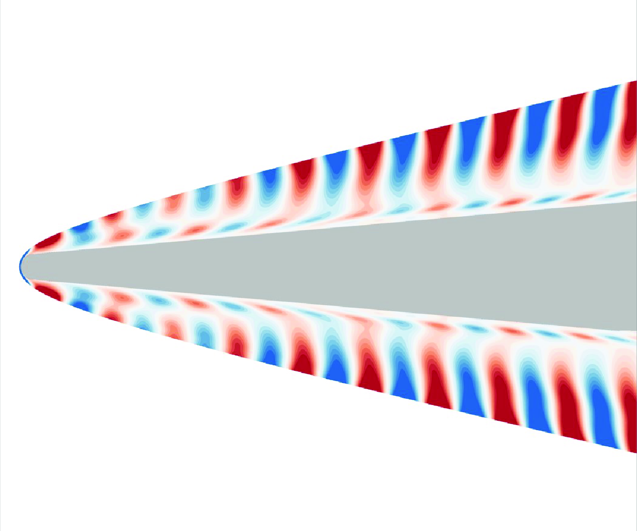
Free-stream slow acoustic waves are considered first. Figure 12 shows the associated density perturbations near the leading edge and behind the shock for $f$ = 600 kHz. The boundary-layer thickness, $\delta$ , as defined through the 99.5 $\,\%$ total enthalpy criterion, is also shown. Two regions can be identified within the disturbance field. The first region is the shock layer, which is defined here as the region between the edge of the boundary layer and the shock. The mean flow in the shock layer is mostly inviscid. By measuring the streamwise wavelengths of the disturbances emanating from the shock, it can be shown that the density perturbations in the shock layer are primarily due to slow acoustic waves. The second region is the boundary layer. The disturbance here is more difficult to characterise based on the perturbation contours alone. A more reliable way to identify the different waves present in the boundary layer is to compute streamwise phase speeds.

Figure 12.

Snapshot of unsteady DNS density perturbation contours near the leading edge for free-stream slow acoustic waves at $f$ = 600 kHz in the TCNE case. The black line represents the boundary-layer thickness defined through the 99.5 $\,\%$ total enthalpy criterion. The contours are clipped to better show disturbance structure.

Figure 13(a) shows the phase speed of the disturbance at the same frequency. The DNS phase speed is computed using the wall pressure perturbation ( $p^{\prime}_w$ ) and the density perturbation ( $\rho '$ ) at $y_n$ = 0.9 mm, which is a position located away from the wall but is close to or within the boundary layer, with the ratio $y_n/\delta$ varying from 1.86 at $s$ = 0.01 m to 0.45 at $s$ = 0.65 m. The phase speed based on the wall pressure perturbation is computed from the FFT output using (4.15). The phase speed based on the density perturbation is estimated from a snapshot of the disturbance field as $c_r \approx 2 f \Delta s_z$ , where $\Delta s_z$ is the distance between successive zeros in the streamwise direction (Fedorov et al. Reference Fedorov, Ryzhov, Soudakov and Utyuzhnikov2013). The phase speed towards the leading edge oscillates about the slow acoustic spectrum or the entropy/vorticity spectrum, depending on the wall-normal position and the disturbance quantity considered. The former indicates the presence of slow acoustic waves. Since mode $S$ is excited by slow acoustic waves near the leading edge owing to their synchronisation, it can be inferred that mode $S$ is also present. The latter indicates the presence of entropy/vorticity waves. Because of their similar phase speeds, it is not possible to determine whether these waves are primarily entropy waves or vorticity waves, at least within the scope of the present study. Accordingly, we use the term ‘entropy/vorticity waves’ to be inclusive of both wave types.

Figure 13.

Comparison of (a) phase speed and (b) growth rate between unsteady DNS, LST and LPSE for free-stream slow acoustic waves at $f$ = 600 kHz in the TCNE case.

Figure 14 shows the density perturbations further downstream, in the vicinity of the entropy/vorticity/mode $F_1$ synchronisation point at $s$ = 0.5 m. Again, the density perturbations far outside the boundary layer are primarily due to slow acoustic waves, as can be verified by measuring the streamwise wavelengths directly from the contours. Figure 13(a) shows that between $s \approx$ 0.4 and $s \approx$ 0.5 m, the phase speed is close to the entropy/vorticity spectrum, indicating the presence of entropy/vorticity waves. In the vicinity of the synchronisation point mentioned above, we expect mode $F_1$ to be excited by these entropy/vorticity waves.

Figure 14.

Snapshot of unsteady DNS density perturbation contours in the vicinity of the entropy/vorticity/mode $F_1$ synchronisation point for free-stream slow acoustic waves at $f$ = 600 kHz in the TCNE case. The black line represents the boundary-layer thickness defined through the 99.5 $\,\%$ total enthalpy criterion. The contours are clipped to better show disturbance structure.

Note that the phase speed towards the leading edge never oscillates about mode $F_1$ or the fast acoustic spectrum, regardless of wall-normal position or disturbance quantity. Hence, if mode $F_1$ is excited near the leading edge (by fast acoustic waves), it is most likely excited weakly compared with mode $S$ .

The oscillations in phase speed (figure 13a) and growth rate (figure 13b) are similar to those found in many receptivity studies, such as those of Zhong & Ma (Reference Zhong and Ma2006) and Cerminara & Sandham (Reference Cerminara and Sandham2017). These oscillations are likely due to interference between waves of different streamwise wavelengths. However, a strict verification of the underlying mechanism will require the use of multimode decomposition (see Gaydos & Tumin Reference Gaydos and Tumin2004; Miselis, Huang & Zhong Reference Miselis, Huang and Zhong2016 or Zou & Zhong Reference Zou and Zhong2023), which allows one to isolate the amplitude of each of the component modes in the boundary layer.

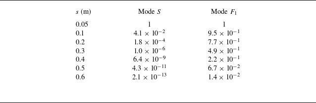
For this flow configuration, mode $S$ is exceptionally stable. This stability is demonstrated in table 2, which shows the LST-derived amplification ratios of modes $S$ and $F_1$ and at various streamwise locations relative to $s$ = 0.05 m for $f$ = 600 kHz. Now, in the LST framework, mode $S$ is always stable. This is not the case in the DNS, where mode $S$ amplifies when excited by other waves in the boundary layer (e.g. by slow acoustic waves near the leading edge) and decays otherwise. Nevertheless, because of its high level of inherent stability, mode $S$ may be attenuated so strongly that it reaches the mode $F_1$ / $S$ synchronisation region (in the vicinity of $s$ = 0.594 m at this frequency) with a much lower amplitude than mode $F_1$ . Now, the relevance of mode $S$ in the receptivity process derives from its synchronisation with mode $F_1$ . If mode $S$ is much weaker than mode $F_1$ , we can effectively treat mode $S$ as if it were not present to begin with. Hence, the excitation of mode $S$ by slow acoustic waves may be secondary, or even irrelevant, in terms of its contribution to the amplitude of mode $F_1$ at the branch I neutral point, compared with the direct excitation of mode $F_1$ (by entropy/vorticity waves and fast acoustic waves).

Table 2.

The LST-derived amplification ratios at various streamwise locations for mode $S$ and mode $F_1$ relative to $s$ = 0.05 m at $f$ = 600 kHz.

The evolution of the boundary-layer disturbance can be understood further by considering the wall pressure perturbation amplitude, as shown in figure 15. At $f$ = 400 kHz, the branch I neutral point is downstream of $s$ = 1.25 m (the end of the domain), and as such, second-mode amplification is not observed. For the remaining frequencies (including those not shown in the figure), two distinct regions can be identified. The first region is upstream of the branch I neutral point. Here, the amplitude generally decreases in the streamwise direction, but is highly oscillatory. There is a noticeable amplification of the disturbance in the vicinity of the entropy/vorticity/mode $F_1$ synchronisation point which is likely due to the interaction between mode $F_1$ and the entropy/vorticity waves. A similar amplification was noted by Fedorov et al. (Reference Fedorov, Ryzhov, Soudakov and Utyuzhnikov2013) in the context of receptivity to temperature spots. The second region is downstream of the branch I neutral point. Here, there is a clear increase in amplitude due to the second-mode instability of mode $F_1$ . At the same time, the amplitude curve becomes smoother as other waves contribute less and less to the overall disturbance.

Figure 15.

Wall pressure perturbation amplitude vs. streamwise distance for free-stream slow acoustic waves at (a) $f$ = 400, (b) $f$ = 600, (c) $f$ = 800 and (d) $f$ = 1000 kHz, in the TCNE and frozen cases. The dash-dot lines indicate the branch I and II neutral points in the TCNE case based on LPSE.

In this study, receptivity coefficients are obtained by backtracking the initial amplitude of mode $F_1$ at the branch I neutral point from its amplitude downstream. This method is described in greater detail in § 7.1.3. To use this method, it is important to determine where mode $F_1$ becomes ‘sufficiently dominant’, a term which we define here to mean that the DNS amplitude approximates the amplitude of mode $F_1$ well enough to backtrack receptivity coefficients reliably. One way to do this is to look at the amplitude plot and find the point downstream of the branch I neutral point where the oscillations are sufficiently weak. Using this criterion, we can say that for 500 kHz $\leqslant f \leqslant$ 900 kHz, mode $F_1$ becomes sufficiently dominant at least by the branch II neutral point. However, for $f$ = 1000 kHz, there are still noticeable oscillations present at the branch II neutral point, implying that mode $F_1$ does not become sufficiently dominant at this frequency. The main drawback with this method is that it is sometimes difficult to determine how strong the oscillations are if the underlying amplitude is increasing, which often limits its applicability to the region in the vicinity of the branch II neutral point.

Because of the difficulty mentioned above, it is sometimes preferable to instead use the phase speed and growth rate plots to estimate the point at which mode $F_1$ becomes sufficiently dominant. The oscillations in these quantities are usually easier to identify than the oscillations in amplitude, and can be easily compared with LST or LPSE results. Returning to figure 13, we find that both the phase speed and growth rate eventually begin to track mode $F_1$ as it becomes amplified via the second-mode instability. The oscillations in both quantities become negligible around $s$ = 0.8 m, which means that mode $F_1$ has become sufficiently dominant at least by this point. After this point, there is decent agreement between the DNS results and the LST mode $F_1$ and LPSE results. Furthermore, the LPSE growth rate matches much more closely with the DNS, since non-parallel effects are included in the LPSE framework.

Figure 16 shows the pressure perturbation profiles at two locations within the unstable region. The first location considered is $s$ = 0.658 m, where there are noticeable discrepancies between the DNS profile and the LST mode $F_1$ and LPSE profiles towards the upper portion of the boundary layer. These discrepancies are due to weak second-mode amplification and the presence of slow acoustic and entropy/vorticity waves. On the other hand, at $s$ = 0.802 m, the DNS profile matches well with the LST mode $F_1$ and LPSE profiles, confirming that mode $F_1$ is sufficiently dominant at this point.

Figure 16.

Comparison of wall-normal pressure perturbation profiles between unsteady DNS, LST and LPSE for free-stream slow acoustic waves at $f$ = 600 kHz in the TCNE case. Panels show (a) $s$ = 0.658 m and (b) $s$ = 0.802 m.

7.1.2. Fast acoustic waves

We now consider fast acoustic waves imposed in the free stream. Figure 17 shows the density perturbations near the leading edge at $f$ = 600 kHz. The density perturbations in the shock layer are primarily due to fast acoustic waves, as confirmed by measuring the streamwise wavelengths of the disturbances emanating from the shock. As before, we compute phase speeds to identify the different types of waves in the boundary layer. Figure 18 shows the estimated phase speed based on the wall pressure perturbation for the same frequency. Other quantities and/or wall-normal positions in the boundary layer show qualitatively similar results. Towards the leading edge, the phase speed oscillates about the phase speed of mode $F_1$ . However, since mode $F_1$ is excited by fast acoustic waves near the leading edge, we can infer that fast acoustic waves are also present in the boundary layer here.

Figure 17.

Snapshot of unsteady DNS density perturbation contours near the leading edge for free-stream fast acoustic waves at $f$ = 600 kHz in the TCNE case. The black line represents the boundary-layer thickness defined through the 99.5 $\,\%$ total enthalpy criterion. The contours are clipped to better show the disturbance structure.

Figure 18 also shows the phase speed of mode $F_2$ . This mode belongs to the same family of modes as mode $F_1$ . However, mode $F_2$ exits the fast acoustic spectrum much further downstream than mode $F_1$ . The line labelled ‘mode $F_2$ ’ corresponds to both a fast acoustic mode and mode $F_2$ . Towards the leading edge, the LST solver seems to track a fast acoustic mode, which explains the rapid increase in phase speed past $c_r/u_{ps}$ = $1 + 1/M_{ps}$ there. It is unclear where the line transitions from a fast acoustic mode to mode $F_2$ , i.e. where mode $F_2$ emerges from the fast acoustic spectrum as a distinct mode. Therefore, if the DNS phase speed is close to the fast acoustic spectrum, it may indicate the presence of (i) fast acoustic waves only or (ii) a combination of fast acoustic waves and mode $F_2$ , depending on the streamwise location.

Figure 18.

Comparison of phase speed between unsteady DNS, LST and LPSE for free-stream fast acoustic waves at $f$ = 600 kHz in the TCNE case. The DNS and LPSE results are obtained using the wall pressure perturbation.

Moving downstream from the leading edge, the phase speed eventually shifts away from mode $F_1$ and towards the fast acoustic spectrum. This behaviour is explained by the fact that mode $F_1$ begins to decay at some point downstream owing to its gradual desynchronisation with the fast acoustic waves, and because mode $F_1$ is nominally stable upstream of the branch I neutral point. Hence, the amplitude of mode $F_1$ becomes lower than the amplitude of the fast acoustic waves or, if mode $F_2$ is also present, their combined amplitudes (i.e. the sum of their amplitudes). This causes the phase speed to shift towards the fast acoustic spectrum.

Moving even further downstream towards the entropy/vorticity/mode $F_1$ synchronisation point at $s \approx$ 0.5 m, the phase speeds remain close to the fast acoustic spectrum, indicating that the waves in the boundary layer continue to primarily be fast acoustic waves or a mixture of fast acoustic waves and mode $F_2$ .

In this case, the oscillations in phase speed (and amplitude) are consistent with interference between mode $F_1$ and fast acoustic waves (or a mixture of fast acoustic waves and mode $F_2$ ). This will be shown later. For now, it suffices to say that, near the leading edge, the presence of mode $S$ should cause secondary oscillations of very short length scales due to the large wavelength difference between mode $S$ and the waves mentioned earlier. Such oscillations are not observed here, which indicates that mode $S$ , if present, is very weak compared with mode $F_1$ . Combined with the fact that mode $S$ is highly stable (see discussion in § 7.1.1), the excitation of mode $S$ by slow acoustic waves is unlikely to be a relevant receptivity mechanism in this case. On a separate note, the decay of mode $F_1$ moving downstream from the leading edge could allow it to interact with weak entropy/vorticity waves as it synchronises with the entropy/vorticity spectrum. Because of the strong oscillations in amplitude due to interference (see figure 19), it is difficult to tell if there is any local amplification that would indicate an interaction between mode $F_1$ and the entropy/vorticity waves. Hence, it is unclear whether the excitation of mode $F_1$ by entropy/vorticity waves is significant.

Figure 19.

Wall pressure perturbation amplitude vs. streamwise distance for free-stream fast acoustic waves at (a) $f$ = 400, (b) $f$ = 600, (c) $f$ = 800 and (d) $f$ = 1000 kHz, in the TCNE and frozen cases. The dash-dot lines indicate the branch I and II neutral points in the TCNE case based on LPSE.

The wall pressure perturbation amplitudes for the fast acoustic wave case are presented in figure 19. For $f$ = 400 kHz, there is no observed second-mode amplification, since the branch I point is downstream of the end of the domain. For $f$ = 500 kHz (not shown) and $f$ = 600 kHz, second-mode amplification can be clearly identified, but there are strong oscillations well into the unstable region, unlike what was found in the slow acoustic wave case. These oscillations (which can be found for all considered frequencies) are due to interference between mode $F_1$ and fast acoustic waves (or a mixture of fast acoustic waves and mode $F_2$ ). The persistence of these oscillations up to the branch II neutral point implies that mode $F_1$ never becomes sufficiently dominant. However, for these two frequencies (500 and 600 kHz), mode $F_1$ does at least surpass the combined amplitude of the other waves through second-mode amplification. This is demonstrated in figure 18, where the phase speed at $f$ = 600 kHz shifts towards that of mode $F_1$ around $s$ = 0.85 m.

Figure 20 compares the DNS pressure perturbation profiles with the LST/LPSE results for several streamwise locations near $s$ = 1 m for $f$ = 600 kHz. These locations correspond to different points along the oscillations in wall pressure perturbation amplitude, as shown in the inset of the figure. For brevity, the LST and LPSE profiles are shown only for $s$ = 1.0021 m, keeping in mind that the LST and LPSE profiles do not change significantly between the locations considered. The effect of interference on the perturbation throughout the boundary layer is seen through the differences in the shapes of the DNS profiles between these locations. The DNS profiles show poor overall agreement with the LST mode $F_1$ eigenfunction and the LPSE shape function, confirming that mode $F_1$ does not become sufficiently dominant despite second-mode amplification.

Figure 20.

Comparison of wall-normal pressure perturbation profiles between unsteady DNS, LST and LPSE near $s$ = 1 m for free-stream fast acoustic waves at $f$ = 600 kHz in the TCNE case.

For $f \geqslant$ 700 kHz, second-mode amplification is weak enough that mode $F_1$ never surpasses the combined amplitude of the other waves. Accordingly, the phase speed at these frequencies (not shown) does not shift towards that of mode $F_1$ even after second-mode amplification. This result, combined with the observation that the location of the apparent peak disagrees with that of the branch II neutral point, suggests that the amplification seen in figure 19 for $f$ = 800 and 1000 kHz is unrelated to second-mode amplification. However, Ma & Zhong (Reference Ma and Zhong2003a , Reference Ma and Zhongb ) and Zhong & Ma (Reference Zhong and Ma2006) found that there can be a notable downstream amplification due to the excitation of mode $F_2$ by fast acoustic waves (owing to their synchronisation). This is likely the case here.

An interesting observation is that for $f$ = 1000 kHz, the amplitude curve is fairly smooth past $s \approx$ 0.2 m. Now, since the oscillations are due to interference between mode $F_1$ , fast acoustic waves and mode $F_2$ (as will be shown later), it can be concluded that the observed smoothness past $s \approx$ 0.2 m is due to the fast acoustic waves (or the combination of fast acoustic waves and mode $F_2$ ) being particularly strong compared with the amplitude of mode $F_1$ , which undergoes weak second-mode amplification at this frequency.

It is possible to directly verify that the oscillations in amplitude are due to interference between waves. If a disturbance consists of two waves with different phase speeds, the expression given by De Tullio & Sandham (Reference De Tullio and Sandham2015) can be used to estimate the peak-to-peak distance in the oscillations of the disturbance amplitude owing to their interference. This expression is written as

(7.1) \begin{equation} \Delta s = \frac {c_{r,A}c_{r,B}}{f |c_{r,A}-c_{r,B}|}, \end{equation}

where $\Delta s$ is the peak-to-peak distance and $c_{r,A}$ and $c_{r,B}$ are the phase speeds of waves A and B, respectively. Consider wave A to have a phase speed near the fast acoustic spectrum, so that $c_{r,A} \approx$ 1.205 $u_{\!ps}$ . Consider wave B to be mode $F_1$ , keeping in mind that $c_{r,B}$ must be adjusted according to the local phase speed of mode $F_1$ . The peak-to-peak distance shown in the inset of figure 19(b) for $f$ = 600 kHz is measured to be approximately 16.3 mm. Using the above expression with the phase speed of mode $F_1$ evaluated at the midpoint of the two peaks, the peak-to-peak distance is approximately 16.2 mm, showing excellent agreement with the DNS results. The agreement at other locations is not quite as good, but still decent overall. The relative error is approximately 9 $\,\%$ for the first set of peaks near the leading edge, 5 $\,\%$ for the second set and so on, continuing to decrease downstream. This indicates that the oscillations are due to interference between mode $F_1$ and a wave (or a combination of waves) whose phase speed(s) is (are) close to the fast acoustic spectrum. In other words, the oscillations are due to interference between mode $F_1$ and the fast acoustic waves or, if mode $F_2$ is present, a combination of both waves. A similar analysis can be performed for the phase speed plots.

The origin of the oscillations is the same for all considered frequencies. However, a notable exception is that there are long-period oscillations that appear some distance downstream of the branch II neutral point at higher frequencies (see the amplitude curves for $f$ = 800 and 1000 kHz in figure 19). These oscillations are instead more consistent with interference between mode $F_2$ and the fast acoustic waves.

7.1.3. Receptivity coefficients

A key objective in a receptivity study is to obtain receptivity coefficients. Generally, the receptivity coefficient (denoted by $C_R$ ) is defined as $C_R$ = $A_0/A_\infty$ , where $A_0$ is the amplitude of the unstable mode at the branch I neutral point, and $A_\infty$ is the amplitude of the free-stream disturbance. Unfortunately, obtaining $A_0$ is not straightforward, since the boundary-layer disturbance in the DNS contains many competing modes at the branch I neutral point. However, it is still possible to estimate the receptivity coefficient by using a backtracking method, as Ma & Zhong (Reference Ma and Zhong2003b ) have done. The premise of this method is that if the amplitude of the unstable mode is known at some point downstream of the branch I neutral point, then dividing that amplitude by the corresponding $N$ -factor at the point allows for the branch I amplitude to be estimated. Rearranging (4.9), the branch I amplitude of the unstable mode can be estimated as

(7.2) \begin{equation} A_0 = A(s_0) = \frac {A(s)}{\int _{s_0}^{s} \sigma (s) \,ds} = \frac {A(s)}{e^{N(s)}} .\end{equation}

Here, the amplitude $A$ is obtained by sampling the unsteady DNS perturbation at some point downstream of the branch I neutral point where the unstable mode is sufficiently dominant. The value of $e^N$ at the same point can be obtained from LST or LPSE. As mentioned before, the location at which the unstable mode becomes sufficiently dominant can be found by looking at the amplitude, phase speed or growth rate plots. We expect that mode $F_1$ reaches its highest amplitude, and is hence most dominant, near the branch II neutral point. Therefore, the sampling location is taken to be the branch II neutral point (as predicted by the LPSE) except in cases where the branch II neutral point is outside the computational domain, in which case the last point in the domain is used. Here, the receptivity coefficient is evaluated using the wall pressure perturbation amplitude normalised by the free-stream pressure perturbation amplitude, so that $C_R$ = $|p^{\prime}_w(s_0)|/|p^{\prime}_\infty |$ .

A major limitation to the methodology described above is that, for a given frequency, there must exist a location where the unstable mode is sufficiently dominant in the DNS. An exception to this is that, if the unstable mode is greater than the combined amplitude of the other waves, but not sufficiently dominant, the phase speed and growth rate tend to oscillate about the solution for the unstable mode. This was, for example, seen for $f$ = 600 kHz in the fast acoustic wave case (figure 18). In this scenario, it is possible to filter out the oscillations and approximately recover the amplitude of mode $F_1$ by using a smoothing algorithm.

The smoothing is performed using the locally estimated scatterplot smoothing method of Cleveland & Devlin (Reference Cleveland and Devlin1986). This method requires the user to specify a window length, denoted by $L$ , on which the smoothing is performed. The ratio of $L$ to the length scale of the oscillations/variations in amplitude determines the level of smoothing, with large ratios corresponding to more smoothing and vice versa. The relevant oscillation length scale is the peak-to-peak distance (denoted by $\Delta s$ ), which can be estimated at a given sampling location by using (7.1) or by direct measurement. Figure 21(a) shows the amplitude plotted versus $L/\Delta s$ at the branch II neutral point (predicted by LPSE) in the fast acoustic wave case at $f$ = 600 kHz. Because the unsmoothed amplitude is near a local minimum in the oscillations, increasing $L$ initially leads to a sharp increase in amplitude. Also, since the oscillations have a relatively short length scale, they become damped with small $L$ . However, since the underlying amplitude variation of mode $F_1$ occurs over much longer length scales, $L$ must be increased substantially before mode $F_1$ itself is damped. Based on this observation, the optimal $L$ presumably lies in the region immediately after the oscillations have been damped. For the case shown in figure 21(a), we chose $L/\Delta s$ = 8 (shown as the vertical dashed line) as the window length. The smoothed amplitude curves for this case are shown in figure 21(b) for different values of $L/\Delta s$ . Reasonable values of $L/\Delta s$ seem to vary between 6 and 8 for the other fast acoustic wave cases. We used $L/\Delta s$ = 5 in the slow acoustic wave case for $f$ = 1000 kHz. As an additional verification of the smoothing procedure, we applied it to the slow acoustic wave case at $f$ = 600 kHz, where oscillations near the branch II neutral point are negligible to begin with. Now, in this study, the largest $L$ relative to the underlying variation of mode $F_1$ , i.e. the strongest smoothing, corresponds to $L/\Delta s$ = 5 in the slow acoustic wave case at $f$ = 1000 kHz. For the purposes of this verification we can obtain a roughly equivalent peak-to-peak distance for $f$ = 600 kHz by taking the peak-to-peak distance near the branch II neutral point in the slow acoustic wave case at $f$ = 1000 kHz and multiplying it by 5/3, the ratio of the two frequencies. Figure 21(c) shows the result. It is evident that even the strongest smoothing has a negligible effect on the amplitude of mode $F_1$ itself.

Figure 21.

(a) Amplitude versus $L/\Delta s$ at the LPSE branch II neutral point (s $\approx$ 1.04 m) in the TCNE fast acoustic wave case at $f$ = 600 kHz. (b) Amplitude curves near the branch II neutral point in the TCNE fast acoustic wave case at $f$ = 600 kHz for several values of $L/\Delta s$ . (c) Unsmoothed and smoothed ( $L/\Delta s$ = 8) amplitude curves near the branch II neutral point in the TCNE slow acoustic wave case at $f$ = 600 kHz.

Using the backtracking method, receptivity coefficients can be computed without smoothing for 500 kHz $\leqslant f \leqslant$ 900 kHz in the slow acoustic wave case or with smoothing for $f$ = 1000 kHz in the slow acoustic wave case and $f$ = 500 and 600 kHz in the fast acoustic wave case. In all other cases, it is not possible to compute receptivity coefficients, at least within the scope of the present study. These cases are $f$ = 400 kHz in both the slow and fast acoustic wave cases, where the unstable region is downstream of the end of the domain, and $f \geqslant$ 700 kHz in the fast acoustic wave case, where mode $F_1$ never exceeds the amplitude of the fast acoustic waves, thus preventing the use of smoothing. Obtaining receptivity coefficients in the latter scenario is likely to require multimode decomposition of the DNS results.

The second-mode receptivity coefficients are shown in figure 22. Only the TCNE case is considered in the present discussion. At $f$ = 500 and 600 kHz, the receptivity coefficients in the fast acoustic wave case are much larger than the slow acoustic wave case. In other words, the fast acoustic waves excite the second mode more strongly than slow acoustic waves at these frequencies. From this result, it would be fair to assume that transition would occur earlier if purely fast acoustic waves were imposed in the free stream rather than slow acoustic waves. However, this is an unrealistic scenario. Recent studies have shown that in hypersonic wind tunnels, the free-stream acoustic waves are primarily slow acoustic waves (Duan, Choudhari & Wu Reference Duan, Choudhari and Wu2014; Wagner et al. Reference Wagner, Schülein, Petervari, Hannemann, Ali, Cerminara and Sandham2018). Another interesting result is that the fast acoustic receptivity coefficient at $f$ = 600 kHz is slightly smaller than at $f$ = 500 kHz, contradicting the results for the slow acoustic waves, where the receptivity coefficients increase with frequency. However, due to the lack of additional data points, it is unclear whether this trend would be continued.

Figure 22.

Second-mode (mode $F_1$ ) receptivity coefficients based on the wall pressure perturbation amplitude. Receptivity coefficients are estimated using the backtracking method with $N$ -factors from LPSE.

7.2. Frozen case

Comparing the unsteady DNS results between the two gas models, we find that in both the slow acoustic wave case (figure 15) and the fast acoustic wave case (figure 19), the amplitude curves are qualitatively similar, indicating that TCNE effects do not fundamentally change the receptivity mechanism. This can also be further verified by looking at the phase speed and growth rate plots, which for brevity are not shown here. However, for the frequencies at which mode $F_1$ surpasses the external waves in amplitude through second-mode amplification ( $f \geqslant$ 500 kHz in the slow acoustic wave case, and $f$ = 500 and 600 kHz in the fast acoustic wave case), the peak amplitudes attained through second-mode amplification are much higher in the TCNE case. For example, in both the slow and fast acoustic waves cases at $f$ = 600 kHz, the peak amplitude is about two times higher using the TCNE gas model.

Figure 22 shows that the receptivity coefficients in the TCNE case show the same frequency-dependent behaviour as the frozen case. This is unsurprising since the receptivity mechanism is essentially unchanged between the two gas models. However, the receptivity coefficients in the TCNE case are smaller by an average of approximately 9 $\,\%$ in the slow acoustic wave case and 8 $\,\%$ in the fast acoustic wave case. Recall, however, that the second mode attains higher peak $N$ -factors in the TCNE case. This means that TCNE effects have competing impacts on receptivity versus stability for the frequencies considered here.

The receptivity coefficients shown in figure 22 were obtained using the wall pressure perturbation amplitude. However, the comparison between the two gas models could change if other disturbance quantities are considered. To investigate this, we can use LST to obtain the eigenfunctions of the second mode at the branch I neutral point and then scale those eigenfunctions based on the wall pressure perturbation amplitude (i.e. the receptivity coefficients in figure 22). If we consider the peak amplitudes of density, streamwise velocity, wall-normal velocity and translation–rotation temperature, the reduction in amplitude in the TCNE case is similar or larger in magnitude compared with the wall pressure perturbation.

Although the destabilisation of the second mode in the TCNE case is due to the cooling of the mean flow, the specific mechanisms behind the reduction in receptivity coefficients is still unclear. A number of mechanisms could be relevant here, namely (i) a weakening of the external waves that excite mode $F_1$ , (ii) a reduction in the efficiency of the receptivity process, which could be characterised by the ratio of the amplitude of mode $F_1$ to the external waves and/or (iii) stronger decay of mode $F_1$ outside the regions where mode $F_1$ is excited. Unfortunately, the DNS results do not provide sufficient information to confirm these effects. For instance, in the slow acoustic wave case, the boundary-layer disturbance using the TCNE gas model is broadly attenuated for a number of key disturbance quantities for much of the flow field upstream of the branch I neutral point, as demonstrated in figure 23. However, the disturbance consists of slow acoustic waves, entropy/vorticity waves and mode $F_1$ , to varying degrees. As such, while it can be concluded that the overall disturbance is weaker in the TCNE case, we cannot make any further conclusions. In the fast acoustic wave case, we have found that the disturbance can either be stronger or weaker in the TCNE case, depending on the disturbance quantity and the streamwise/wall-normal positions. In this case it is unclear whether even the overall disturbance is necessarily stronger or weaker. Further investigation of the mechanisms mentioned above will require the use of multimode decomposition, which is outside of the scope of this study.

Figure 23.

Comparison of disturbance amplitudes based on (a) translation–rotation temperature, (b) pressure, (c) streamwise velocity and (d) density at $s$ = 0.4 m and $f$ = 600 kHz in the slow acoustic wave case.