1 Introduction
Gravity currents occur when a fluid of one density flows primarily horizontally into a fluid of a different density. There are many examples of gravity currents, both naturally occurring and man made (Simpson Reference Simpson1997). Gravity currents propagating along a smooth surface have been extensively studied (e.g. Rottman & Simpson Reference Rottman and Simpson1983; Shin, Dalziel & Linden Reference Shin, Dalziel and Linden2004; Cantero et al.
Reference Cantero, Lee, Balachandar and Garcia2007; Ooi, Constantinescu & Weber Reference Ooi, Constantinescu and Weber2009). However, it is not uncommon for a gravity current to encounter an array of obstacles that provide an additional drag and impede its progress (Hatcher, Hogg & Woods Reference Hatcher, Hogg and Woods2000). The impact of the obstacles is felt over different fractions of the total flow depth depending on their submergence ratio
 $H/h$
, where
 $H$
is the flow depth and
 $h$
is the obstacle height. A handful of previous studies have dealt with the effect of emergent arrays (
 $H/h\leqslant 1$
) on buoyancy-driven exchange flows (e.g. Tanino, Nepf & Kulis Reference Tanino, Nepf and Kulis2005; Jamali, Zhang & Nepf Reference Jamali, Zhang and Nepf2008; Zhang & Nepf Reference Zhang and Nepf2008; Ozan, Constantinescu & Hogg Reference Ozan, Constantinescu and Hogg2015). Nevertheless, the problem of gravity currents interacting with a submerged array (
 $H/h>1$
) has received less attention, partly due to the additional complexity arising from the drag continuity at the array–ambient interface. The propagation and structure of bottom-boundary gravity currents over a sparse array of two-dimensional submerged obstacles have been investigated by Tokyay, Constantinescu & Meiburg (Reference Tokyay, Constantinescu and Meiburg2011, Reference Tokyay, Constantinescu and Meiburg2012, Reference Tokyay, Constantinescu and Meiburg2014). Cenedese, Nokes & Hyatt (Reference Cenedese, Nokes and Hyatt2016) experimentally found that enhancement of the dilution of the gravity current by a submerged array can occur due to two different mechanisms. For a sparse array, the vast majority of the gravity current propagates within the array, and the individual cylinder wakes are the main contributor to the current dilution. In contrast, for a dense array, the gravity current rides on top of the array and the dilution is enhanced by the vertical convective instability arising from the unstable stratification between the dense current and the ambient lighter fluid within the array. The propagation of a surface current beneath a floating array of obstacles has been studied experimentally by Zhang & Nepf (Reference Zhang and Nepf2011) and numerically by Ozan, Constantinescu & Nepf (Reference Ozan, Constantinescu and Nepf2016), which have led to similar results with the studies of bottom currents over a submerged array.
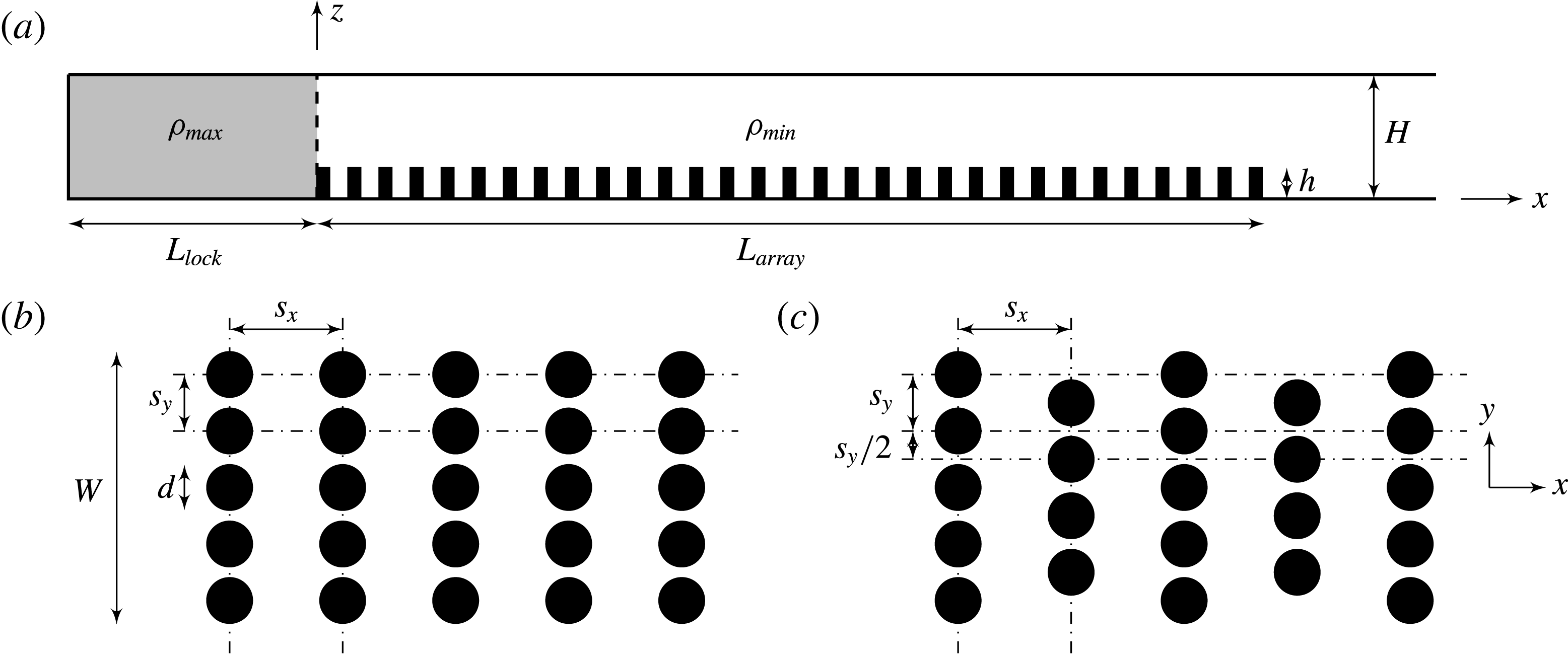
Schematic diagram showing the full-depth lock-exchange set-up used in this study. (a) Elevation view of the channel; (b) plan view of the in-line arrangement; (c) plan view of the staggered arrangement. The vertical dashed line in (a) indicates the gate position at
 $x=0$
. The rightmost end of the array is far from the channel extremity. Circular cylinders (when present) with a diameter of
 $d$
and a height of
 $h$
are mounted on the channel bed, with their axes parallel to the vertical direction. The streamwise and spanwise centre-to-centre cylinder spacings are denoted as
 $s_{x}$
and
 $s_{y}$
, respectively. In the staggered case, the offset rows are shifted by
 $s_{y}/2$
along the spanwise direction. Not to scale.
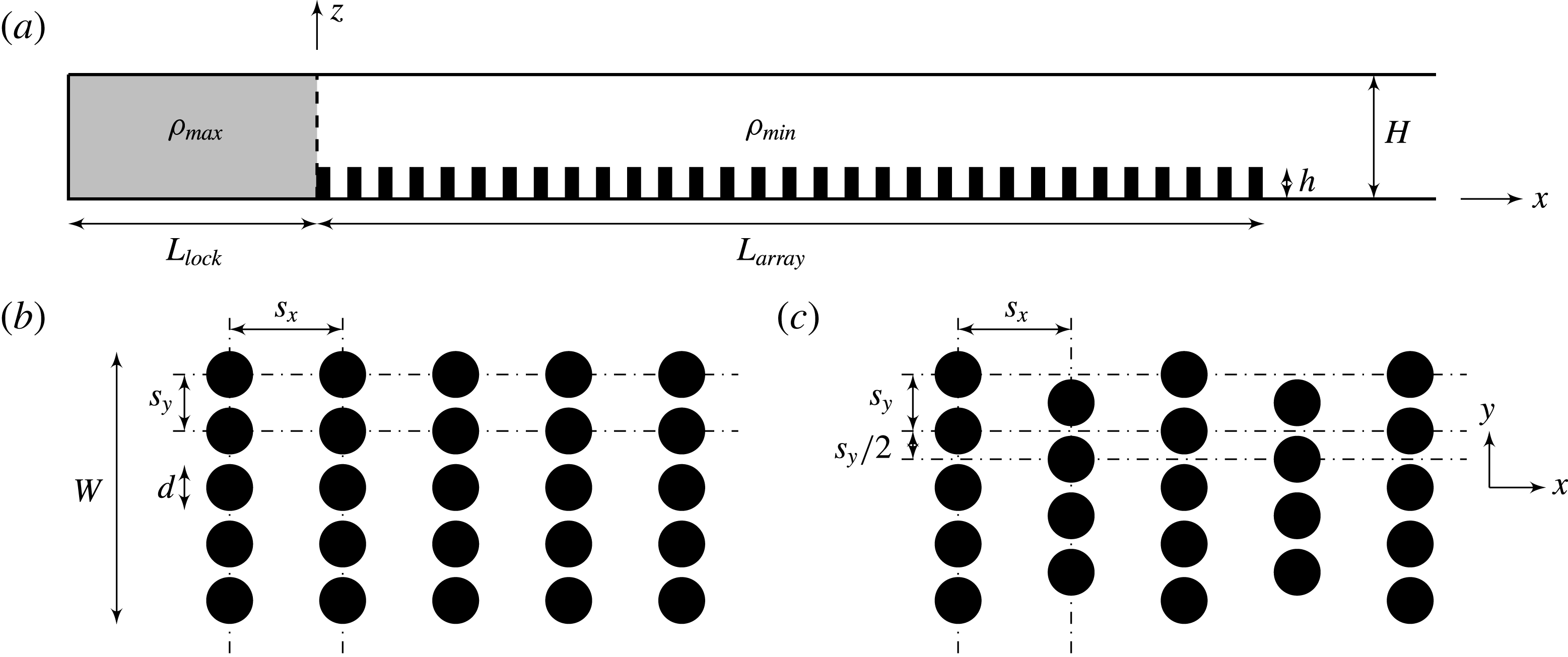
Figure 1 shows the full-depth lock-exchange set-up of a bottom-boundary Boussinesq gravity current propagating over and through a submerged array of circular cylinders used in this study. The initial maximum and minimum fluid densities in the lock and ambient regions before gate removal are denoted as
 $\unicode[STIX]{x1D70C}_{max}$
and
 $\unicode[STIX]{x1D70C}_{min}$
, respectively. The reduced gravity is defined as
 $g^{\prime }=g(\unicode[STIX]{x1D70C}_{max}-\unicode[STIX]{x1D70C}_{min})/\unicode[STIX]{x1D70C}_{max}$
. The channel depth,
 $H$
, and the corresponding buoyancy velocity,
 $u_{b}=\sqrt{g^{\prime }H}$
, are used as the characteristic length and velocity scales, respectively. Time is rendered dimensionless in terms of
 $t_{0}=H/u_{b}$
. The dimensionless fluid density is defined as
 $\unicode[STIX]{x1D70C}=(\unicode[STIX]{x1D70C}_{a}-\unicode[STIX]{x1D70C}_{min})/(\unicode[STIX]{x1D70C}_{max}-\unicode[STIX]{x1D70C}_{min})\in [0,1]$
where
 $\unicode[STIX]{x1D70C}_{a}$
is the absolute fluid density. The dimension of the circular cylinders is fixed throughout this study, i.e.
 $d$
in diameter and
 $h=2.5d$
in height. This results in an aspect ratio of
 $h/d=2.5$
. There are
 $N$
such circular cylinders within the volume of the array (
 $V_{array}=WhL_{array}$
, including pores) and the array density
 $\unicode[STIX]{x1D719}$
is given by
 $$\begin{eqnarray}\unicode[STIX]{x1D719}=\frac{N(\unicode[STIX]{x03C0}/4)d^{2}h}{V_{array}}.\end{eqnarray}$$
Hereinafter, an array will be referred to as equidistant if the spacings between cylinders in the streamwise and spanwise directions are equal (i.e.
 $s_{x}=s_{y}$
), and non-equidistant otherwise (i.e.
 $s_{x}\neq s_{y}$
). We have conducted a combined experimental and numerical investigation to address the following outstanding research questions and the results of this study may have implications for density-driven gravity currents over groups of obstacles in aquatic/geophysical/atmospheric environments. Specifically:
-
(i) How does the behaviour of the gravity current vary over the full range of
 $\unicode[STIX]{x1D719}$
(i.e. from 0 to 1) on encountering a submerged array? Canopies from different systems with different scales exhibit a wide range of
$\unicode[STIX]{x1D719}$
. For aquatic vegetation,
$\unicode[STIX]{x1D719}$
ranges from 0.001 for marsh grasses to 0.45 for mangroves (Nepf Reference Nepf2012). In industrial settings, however, there is an even wider range of
$\unicode[STIX]{x1D719}$
(
$\unicode[STIX]{x1D719}\approx 0$
in the open country and
$\unicode[STIX]{x1D719}\approx 1$
in a dense urban centre). To date, a very limited range of
$\unicode[STIX]{x1D719}$
has been investigated, with the highest being around 0.36 for both emergent and submerged arrays (Zhang & Nepf Reference Zhang and Nepf2008; Cenedese et al.
Reference Cenedese, Nokes and Hyatt2016). There is some consensus that the front velocity of the gravity current decreases as the array is densified to up to
$\unicode[STIX]{x1D719}\approx 0.36$
, regardless of the submergence condition. For the emergent case, it seems unnecessary to extend
$\unicode[STIX]{x1D719}$
even higher since a further decrease of the front velocity of the current due to the increased array drag can be readily expected until it ceases to advance. In contrast, given the additional flow pathway above a submerged array, it is possible for a gravity current to propagate above the array in a similar way to a gravity current propagating over a flat bed as
$\unicode[STIX]{x1D719}$
reaches unity. The associated change of flow regime occurring within the range of
$\unicode[STIX]{x1D719}=0.36{-}1$
that regulates the propagation and structure of the gravity current is non-trivial and has not yet been explored.
-
(ii) What is the appropriate geometrical characterization of a non-equidistant array for correctly quantifying the propagation of a gravity current? Most existing studies are limited to gravity currents interacting with nearly equidistant arrays, using the conventional horizontally averaged array density
$\unicode[STIX]{x1D719}$
(e.g. Tanino et al.
Reference Tanino, Nepf and Kulis2005; Cenedese et al.
Reference Cenedese, Nokes and Hyatt2016). However, arrays of obstacles such as urban canopies, crop canopies, forest plantations and engineering retarding facilities, are sometimes non-equidistantly distributed. To this end, we propose a new two-dimensional parameter space in which
$\unicode[STIX]{x1D719}$
is further decomposed into its streamwise and spanwise components respectively as (1.2a,b )Physically,
$$\begin{eqnarray}\unicode[STIX]{x1D707}_{x}=d/s_{x}\quad \text{and}\quad \unicode[STIX]{x1D707}_{y}=d/s_{y}.\end{eqnarray}$$
$\unicode[STIX]{x1D707}_{x}$
can be interpreted as a wake parameter, with large
$\unicode[STIX]{x1D707}_{x}$
indicating a strong suppression of the individual cylinder wakes. Meanwhile,
$\unicode[STIX]{x1D707}_{y}$
can be interpreted as an intrusion parameter, with large
$\unicode[STIX]{x1D707}_{y}$
indicating less intrusive flow through the lateral space between cylinders. Accordingly, the original array density can be expressed for circular cylinders as (1.3)
$$\begin{eqnarray}\unicode[STIX]{x1D719}=\left(\frac{\unicode[STIX]{x03C0}}{4}\right)\unicode[STIX]{x1D707}_{x}\unicode[STIX]{x1D707}_{y}.\end{eqnarray}$$





Our study will illustrate the necessity of this directional decomposition of
 $\unicode[STIX]{x1D719}$
for non-equidistant arrays in order to provide an unambiguous description of the gravity current propagation. Note that
 $\unicode[STIX]{x1D719}_{max}=\unicode[STIX]{x03C0}/4$
when the individual cylinders are stacked against each other. Hence, the case with
 $\unicode[STIX]{x1D719}=1$
is realized by replacing the cylinder array with a solid slab of the same height.
The layout of this paper is as follows. The experimental and numerical set-ups, comparison of results as well as the list of large eddy simulation (LES) runs that were performed for a broad-range parametric study are given in § 2. In subsequent sections, the numerical simulation results are presented and discussed. In § 3 we discuss the time-averaged gravity current front velocity during the slumping phase using the
 $\unicode[STIX]{x1D707}_{x}$
–
 $\unicode[STIX]{x1D707}_{y}$
parameterization. We then describe in detail the various flow regimes identified in this study in § 4 and discuss the dynamics associated with each regime change in § 5. Finally, § 6 provides some concluding comments and the relevance of our findings to practical situations.
2 Descriptions of experiments and simulations
2.1 Experimental set-up
A set of laboratory experiments using a similar apparatus to that of Cenedese et al. (Reference Cenedese, Nokes and Hyatt2016) was conducted in this study. As shown in figure 1, a gravity current was generated through the classic lock-exchange configuration in a flat flume with Perspex lateral walls and a glass bottom. The flume was 620 cm in length, 25 cm in width and 50 cm in height. A stainless steel gate sealed by plastic foam was located
 $L_{lock}=100~\text{cm}$
from the left hand end of the flume, partitioning it into two regions: the lock region and the open region containing the roughness elements which extended
 $L_{array}=300~\text{cm}$
away from the gate. The array consisted of vertical rigid plastic cylinders that were 2 cm in diameter and 5 cm in height which are fixed for all the experiments, resulting in a cylinder aspect ratio of
 $h/d=2.5$
. The cylinders were held in place by a perforated aluminium base plate and could be screwed in and out to create different geometrical configurations with varying
 $\unicode[STIX]{x1D707}_{x}$
,
 $\unicode[STIX]{x1D707}_{y}$
and arrangement patterns as indicated in figure 1.
A
 $4~\text{g}~\text{l}^{-1}$
salt solution (
 $\unicode[STIX]{x1D70C}_{max}=1.0014~\text{g}~\text{cm}^{-3}$
) and a
 $14.7~\text{ml}~\text{l}^{-1}$
ethanol solution (
 $\unicode[STIX]{x1D70C}_{min}=0.9963~\text{g}~\text{cm}^{-3}$
) were filled into the lock region and the ambient fluid region, respectively, resulting in a reduced gravity of
 $g^{\prime }=5~\text{cm}~\text{s}^{-2}$
so that the flow could be considered as Boussinesq. The purpose of using an ethanol solution as opposed to fresh water for the ambient fluid was to match its refractive index with the lock fluid (
 $n=1.3337$
) in order to eliminate optical distortions. The densities were measured with an Anton Paar DMA 5000 density meter. The experiment was started by pulling the gate vertically out of the tank. The flow evolution was captured using a JAI BB-141GE (Bayer colour) CCD camera recording at a frame rate of 30.128 Hz. The
 $1392\times 1040$
pixel images were transferred directly to a fast hard drive on a PC during capture. A mirror was used to increase the distance between the camera and the field of view, thus decreasing the impact of parallax. Both the light and dense fluids were seeded with approximately neutrally buoyant Pliolite particles sized at 250–
 $300~\unicode[STIX]{x03BC}\text{m}$
. An LED lightbank generated an approximately 1 cm wide lightsheet which illuminated a slice of the flow from above along the centreline of the tank. The field of view of the camera was from
 $x=77.9{-}128.1~\text{cm}$
, which is referred to as the illuminated region. Enough particles were added to ensure that there were at least 1000 particles in the camera window with a volume of roughly 502 mm
 $\times$
10 mm
 $\times$
 $H$
. The post-processing of the captured images was undertaken using a particle tracking velocimetry technique with the Streams software system (Nokes Reference Nokes2016).
In this study, a total of 11 laboratory experiments were conducted with bottom roughness present. The streamwise array density was varied as
 $\unicode[STIX]{x1D707}_{x}=0.090$
, 0.181 and 0.363 while the spanwise array density was fixed at
 $\unicode[STIX]{x1D707}_{y}=0.636$
, resulting in an array density of
 $\unicode[STIX]{x1D719}=0.045$
, 0.090 and 0.181, respectively. For each array geometry, the water depth was varied to simulate different submergence ratios at
 $H/h=3$
, 4, 5.4 and 7. The data of
 $\unicode[STIX]{x1D719}=0.045$
associated with
 $H/h=7$
were not recorded. It is acknowledged that there are intrinsic problems in obtaining robust time-averaged velocity fields using data recorded by a camera fixed in the laboratory frame of reference. The primary reasons for this are firstly, that it must be assumed that the current is in a quasi-steady state such that the current front propagates at a constant speed and that the internal flow is statistically stationary during the recorded motion; and secondly, that the recording period is sufficiently long to be able to compute robust Reynolds averages in the frame of reference of the current nose. However, comparison of the vertical profiles of the horizontal velocity for three repeated experiments with the same initial conditions (not shown) provides confidence that the experimental results presented in this paper are robust.
2.2 Numerical methodology
The LES filtered Navier–Stokes equations for time-dependent, three-dimensional, incompressible stratified flows with the Boussinesq approximation are given in tensor notation by
 $$\begin{eqnarray}\frac{\unicode[STIX]{x2202}u_{i}}{\unicode[STIX]{x2202}t}+\frac{\unicode[STIX]{x2202}(u_{i}u_{j})}{\unicode[STIX]{x2202}x_{j}}=-\frac{1}{\unicode[STIX]{x1D70C}_{0}}\frac{\unicode[STIX]{x2202}p}{\unicode[STIX]{x2202}x_{i}}+\unicode[STIX]{x1D708}\frac{\unicode[STIX]{x2202}^{2}u_{i}}{\unicode[STIX]{x2202}x_{j}\unicode[STIX]{x2202}x_{j}}-g\frac{\unicode[STIX]{x1D70C}}{\unicode[STIX]{x1D70C}_{0}}\unicode[STIX]{x1D6FF}_{i3}-\frac{\unicode[STIX]{x2202}\unicode[STIX]{x1D70F}_{ij}^{SGS}}{\unicode[STIX]{x2202}x_{j}},\end{eqnarray}$$
subject to the filtered continuity equation
 $$\begin{eqnarray}\frac{\unicode[STIX]{x2202}u_{i}}{\unicode[STIX]{x2202}x_{i}}=0,\end{eqnarray}$$
and the filtered density transport equation
 $$\begin{eqnarray}\frac{\unicode[STIX]{x2202}\unicode[STIX]{x1D70C}}{\unicode[STIX]{x2202}t}+\frac{\unicode[STIX]{x2202}(\unicode[STIX]{x1D70C}u_{j})}{\unicode[STIX]{x2202}x_{j}}=\unicode[STIX]{x1D705}\frac{\unicode[STIX]{x2202}^{2}\unicode[STIX]{x1D70C}}{\unicode[STIX]{x2202}x_{j}\unicode[STIX]{x2202}x_{j}}-\frac{\unicode[STIX]{x2202}\unicode[STIX]{x1D712}_{j}^{SGS}}{\unicode[STIX]{x2202}x_{j}},\end{eqnarray}$$
where
 $u_{i}$
are the Cartesian components of the filtered velocity field,
 $p$
is the filtered pressure,
 $\unicode[STIX]{x1D70C}$
is the filtered density,
 $\unicode[STIX]{x1D70C}_{0}$
is a characteristic reference density,
 $g$
is the gravitational acceleration,
 $\unicode[STIX]{x1D6FF}_{i3}$
is the Kronecker delta,
 $\unicode[STIX]{x1D708}$
is the kinematic viscosity and
 $\unicode[STIX]{x1D705}$
is the molecular diffusivity of the dissolved species that gives rise to the density variation. The spatial filtering operation is not written explicitly. Time is represented by
 $t$
and the index
 $i=1,2,3$
indicates the
 $x$
(streamwise),
 $y$
(spanwise) and
 $z$
(vertical) directions, respectively. The two flow parameters arising from the non-dimensionalization of the governing equations are the channel Reynolds number
 $Re_{H}=u_{b}H/\unicode[STIX]{x1D708}$
and the molecular Schmidt number
 $Sc=\unicode[STIX]{x1D708}/\unicode[STIX]{x1D705}$
.
The governing equations are solved using the finite-volume computational fluid dynamics software, FLOW-3D, developed by Flow Science, Inc. at Santa Fe, New Mexico. It has been extensively validated for various fluid dynamics problems from both academic and engineering perspectives (e.g. Savage & Johnson Reference Savage and Johnson2001; An, Julien & Venayagamoorthy Reference An, Julien and Venayagamoorthy2012; Oertel & Schlenkhoff Reference Oertel and Schlenkhoff2012; Zhou & Venayagamoorthy Reference Zhou and Venayagamoorthy2017). The closure of the subgrid-scale (SGS) stress tensor
 $\unicode[STIX]{x1D70F}_{ij}^{SGS}$
and the subgrid-scale scalar flux vector
 $\unicode[STIX]{x1D712}_{j}^{SGS}$
in equations (2.1) and (2.3) are solved using the Smagorinsky model (Smagorinsky Reference Smagorinsky1963). The turbulent Schmidt number,
 $Sc_{t}$
, is kept at unity which is common in numerical studies of turbulent flows. The unique volume-of-fluid method (Hirt & Nichols Reference Hirt and Nichols1981) of FLOW-3D provides an accurate way to track and locate the free surface or fluid–fluid interface using structured meshes, which consists of three ingredients: a scheme to locate the surface, an algorithm to track the surface as a sharp interface moving through a computational grid and a means of applying boundary conditions at the surface. Besides this, the fractional area-volume obstacle representation technique (Hirt Reference Hirt1993) used exclusively in FLOW-3D enables the model to change the embedded geometry realistically without changing the mesh, which is considered superior for the present study where a broad parametric study of geometric variation is undertaken. The second-order, monotonicity-preserving upwind-differencing method (van Leer Reference van Leer1977) is applied to approximate the momentum and density advection. The pressure is solved implicitly using the generalized minimum residual algorithm due to its high accuracy, rapid convergence and parallel efficiency (Yao Reference Yao2004).
2.3 Comparison of experimental and numerical results
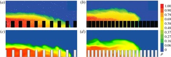
Figure 2 compares the numerical density fields with experiments (Cenedese et al.
Reference Cenedese, Nokes and Hyatt2016) having the same array geometries. Two typical flow structures for a gravity current propagating past a submerged array under a submergence ratio of
 $H/h=4$
are shown. As described in detail in Cenedese et al. (Reference Cenedese, Nokes and Hyatt2016), for the sparse array (figure 2
a,c), the gravity current propagates along the channel bed which resembles the classical case for a smooth bottom. The turbulent cylinder wakes are the main contributor to the dilution of the gravity current. In contrast, for the dense array (figure 2
b,d), the array drag is large enough such that a new, well-defined current nose is found to propagate along the array top. The over-current nose is well mixed with the underlying lighter fluid via vertical convective instability.
Comparison of experimental and numerical instantaneous laterally averaged density fields of a gravity current propagating past a sparse and a dense array. The submergence condition is fixed at
 $H/h=4$
. (a) Sparse, experimental; (b) dense, experimental; (c) sparse, LES; (d) dense, LES. For the sparse array,
 $\unicode[STIX]{x1D707}_{x}=0.361$
,
 $\unicode[STIX]{x1D707}_{y}=0.313$
and
 $\unicode[STIX]{x1D719}=0.09$
. For the dense array,
 $\unicode[STIX]{x1D707}_{x}=0.722$
,
 $\unicode[STIX]{x1D707}_{y}=0.626$
and
 $\unicode[STIX]{x1D719}=0.36$
. The experimental density fields are from Cenedese et al. (Reference Cenedese, Nokes and Hyatt2016).

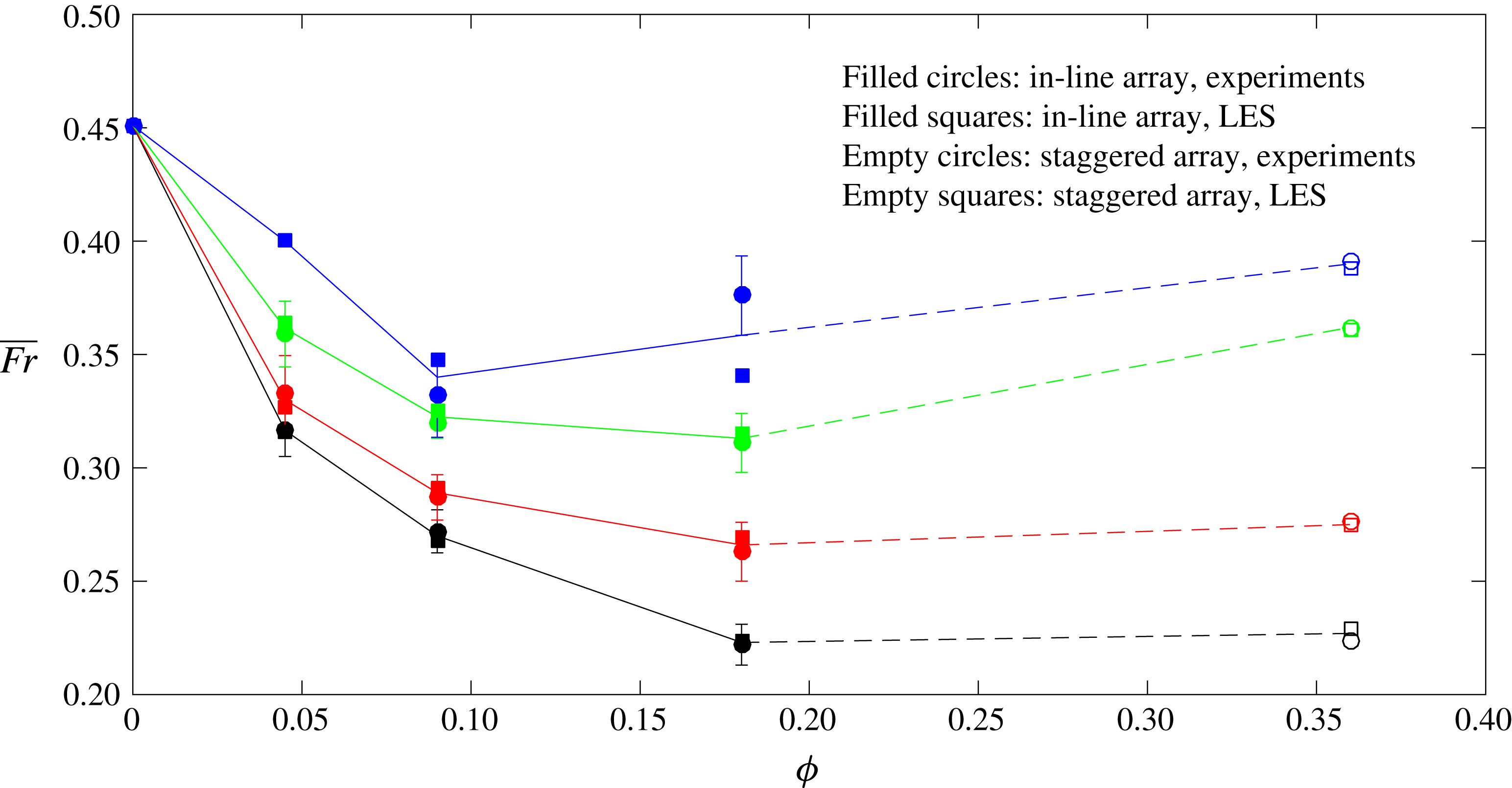
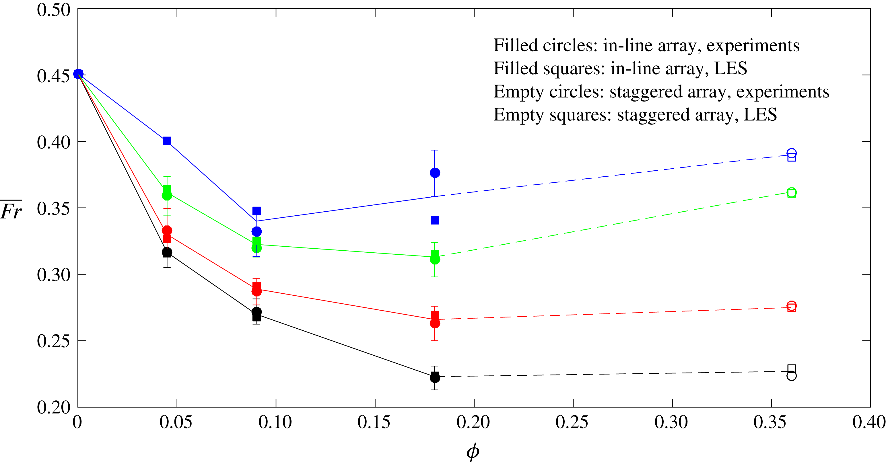
Comparison of the time-averaged Froude number between the laboratory experiments and the numerical simulations for different array densities and submergence conditions (black:
 $H/h=3$
; red:
 $H/h=4$
; green:
 $H/h=5.4$
; blue:
 $H/h=7$
). Error bars are included to account for the range of
 $\overline{Fr}$
in 4–6 different experimental runs for measuring the front velocity for each case due to the unsteady nature of the flow. For in-line arrays, the mean values of experimental and LES results are linearly interpolated by solid lines. The data between in-line and staggered arrays are interpolated using dashed lines. Experimental data of the smooth (
 $\unicode[STIX]{x1D719}=0$
) and the densest cases (
 $\unicode[STIX]{x1D719}=0.36$
) are from Cenedese et al. (Reference Cenedese, Nokes and Hyatt2016).
Within the laboratory illuminated section (
 $x=77.9{-}128.1~\text{cm}$
), the gravity current was found to be propagating at a nearly constant speed. The corresponding time-averaged Froude number is given by
 $$\begin{eqnarray}\overline{Fr}=\overline{U_{f}}/u_{b},\end{eqnarray}$$
where
 $\overline{U_{f}}$
is the time-averaged front velocity that was calculated through a linear interpolation to the variation of the front position,
 $x_{f}$
, as a function of time,
 $t$
. It can be seen in figure 3 that the values of
 $\overline{Fr}$
for the numerical simulations and the laboratory experiments are in excellent agreement to up to
 $\unicode[STIX]{x1D719}=0.36$
, except for the case with
 $\unicode[STIX]{x1D719}=0.181$
and
 $H/h=7$
. Starting from the canonical case of gravity currents propagating over a flat bottom,
 $\overline{Fr}$
is initially seen to decrease as the array becomes denser, which is consistent with gravity current front speeds in emergent canopies (Zhang & Nepf Reference Zhang and Nepf2008) and sparse submerged canopies (Cenedese et al.
Reference Cenedese, Nokes and Hyatt2016). As
 $\unicode[STIX]{x1D719}$
increases further, our laboratory experiments indicate for the first time a non-monotonic dependence of
 $\overline{Fr}$
on
 $\unicode[STIX]{x1D719}$
, and this is confirmed by the numerical simulations. However, the detailed
 $\overline{Fr}\sim \unicode[STIX]{x1D719}$
relationship and the underlying flow physics within the range of
 $\unicode[STIX]{x1D719}=0.36{-}1$
are still unknown. This serves as one of the motivations of the present study.
2.4 Description of the parametric study using LES
A broad-range parametric study is performed using the array characterization method given by equation (1.2a,b
). The initial lock-gate position is at
 $x=0$
, as shown in figure 1. An array of vertical cylinders with an aspect ratio of 2.5 is mounted on the channel bed, with the upstream face of the first row of cylinders located at
 $x=0$
so that the interaction between the gravity current and the array occurs immediately after the gate removal. The streamwise dimension of the array is determined in each simulation to ensure a negligible effect from the downstream boundary of the computational domain. The density difference was kept the same as in the experiments.
The simulation runs performed for the parametric study are summarized in table 1. The submergence ratio is fixed at
 $H/h=5.4$
throughout all the simulations. The flat-bed case (
 $\unicode[STIX]{x1D719}=0$
) and the solid-slab case (
 $\unicode[STIX]{x1D719}=1$
) are regarded as two baseline simulations with the notation
 $$\begin{eqnarray}\text{F-}0\quad \text{and}\quad \text{F-}1,\end{eqnarray}$$
respectively. The simulations with circular cylinders are denoted as
 $$\begin{eqnarray}\text{I(S)-}\unicode[STIX]{x1D707}_{x}\text{-}\unicode[STIX]{x1D707}_{y},\end{eqnarray}$$
where I indicates in-line arrays and S indicates staggered arrays, respectively. The parameters
 $\unicode[STIX]{x1D707}_{x}$
and
 $\unicode[STIX]{x1D707}_{y}$
had values 0.181, 0.272, 0.363, 0.454, 0.545, 0.636, 0.727, 0.818, 0.909 and 1.000, and
 $\unicode[STIX]{x1D707}_{x}$
had an additional value
 $\unicode[STIX]{x1D707}_{x}=0.090$
. We vary
 $\unicode[STIX]{x1D707}_{x}$
and
 $\unicode[STIX]{x1D707}_{y}$
independently such that 110 simulations are conducted for in-line and staggered arrangements, respectively (220 in total). As
 $\unicode[STIX]{x1D707}_{x}$
and
 $\unicode[STIX]{x1D707}_{y}$
vary, the corresponding array density,
 $\unicode[STIX]{x1D719}$
, ranges from 0 to
 $\unicode[STIX]{x03C0}/4$
according to equation (1.3).
List of simulations performed for the parametric study.

This extensive parametric study is made possible at the cost of sacrificing some of the grid resolution. The uniform mesh size of
 $0.2d$
that was used for comparison with the experimental data (figures 2 and 3) is applied to the whole computational domain. A grid-independence study was performed where the grid size was halved to
 $0.1d$
, and the difference of the front velocity was found to be less than
 $5\,\%$
. For most simulations, the number of grid points was
 $1300\times 60\times 80$
in the streamwise (
 $L_{x}=23H$
), spanwise (
 $L_{y}=0.9H$
) and vertical (
 $L_{z}=1.2H$
) directions, respectively. No-slip boundary conditions were employed on the velocity field at the bottom boundary, the upstream and downstream vertical end walls, and on the surfaces of the cylinders. Free-slip boundary conditions are applied to the side walls. The top boundary is modelled as a free surface. The fact that
 $L_{z}$
is slightly larger than
 $H$
is to ensure that free surface fluctuations are accurately modelled by our numerical solver. The time step was automatically adjusted by the solver to be as large as possible without exceeding the stability limits and affecting accuracy, with a mean value of
 $0.003t_{0}$
.
All the LES runs were performed with a channel Reynolds number
 $Re_{H}=u_{b}H/\unicode[STIX]{x1D708}>30\,000$
which is typical for exchange flows within aquatic canopies where
 $Re\sim 10^{4}$
because the current is driven by a small temperature difference due to differential shading. In atmospheric and geophysical settings, however, the Reynolds number is higher (e.g.
 $Re=10^{5}{-}10^{8}$
) due to the increase of the characteristic length and velocity scales. However, we expect the bulk propagation dynamics to be similar, and the
 $Re$
-scaling effects are left to future studies. For most of the simulations, the cylinder Reynolds number
 $Re_{d}=\overline{U}_{f}d/\unicode[STIX]{x1D708}$
was between 500 and 1000 such that the flow can be considered as turbulent and three-dimensional (Williamson Reference Williamson1996).
3 Time-averaged front velocity
For all the simulations listed in table 1, an investigation of the temporal evolution of the gravity current front (not shown) demonstrated that after a short initial acceleration (
 $t=0{-}2t_{0}$
), the gravity current reaches a constant-speed slumping phase (
 $t=2t_{0}{-}21.5t_{0}$
), followed by a buoyancy–inertia self-similar phase within which the current starts to decelerate. In this study, we restrict our discussion to the current propagation in the slumping phase. The Froude number of the frontmost nose (either through or above the array) is defined as
 $$\begin{eqnarray}\overline{Fr}^{\ast }=\text{max}\{\overline{Fr}_{ON},\overline{Fr}_{TN}\},\end{eqnarray}$$
where
 $\overline{Fr}_{ON}$
and
 $\overline{Fr}_{TN}$
are the Froude numbers of the over-nose (ON) above the array and the through-nose (TN) within the array, respectively. The overbar indicates time averaging over
 $t=2t_{0}{-}21.5t_{0}$
, (i.e. during the slumping phase).
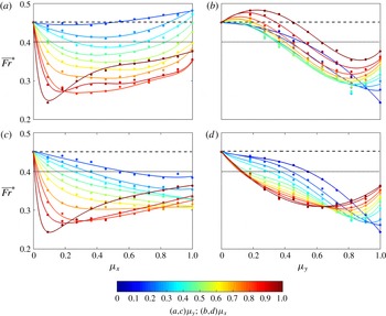
Froude number versus streamwise (spanwise) array density at fixed spanwise (streamwise) array densities. (a,b) In-line arrays; (c,d) staggered arrays. Circles show the values of
 $\overline{Fr}^{\ast }$
in the slumping phase and solid lines are the best fitting curves with
 $R^{2}\geqslant 0.98$
. The two limiting cases are included in each panel: flat-bed case F-0 (- - - -); solid-slab case F-1 (
 $\cdots \,\cdot$
). The submergence ratio is fixed at
 $H/h=5.4$
.

Figure 4 shows the variation of
 $\overline{Fr}^{\ast }$
with
 $\unicode[STIX]{x1D707}_{x}$
or
 $\unicode[STIX]{x1D707}_{y}$
with the other being fixed, for both in-line and staggered arrangements. As discussed in § 5, the two mechanisms leading to the increase of
 $\overline{Fr}^{\ast }$
of the gravity current are the change of regime to either the skimming- or the over-flow regime. For in-line arrays in figure 4(a), the value of
 $\overline{Fr}^{\ast }$
first decreases and then increases with increasing
 $\unicode[STIX]{x1D707}_{x}$
at any fixed
 $\unicode[STIX]{x1D707}_{y}$
. For low-to-moderate
 $\unicode[STIX]{x1D707}_{y}$
, based on the flow regime classification in § 4, the increase of
 $\overline{Fr}^{\ast }$
with increasing
 $\unicode[STIX]{x1D707}_{x}$
is the consequence of a through-to-skimming regime change (see § 5.2.1). On the other hand, for large
 $\unicode[STIX]{x1D707}_{y}$
, the streamwise densification of the array results in a much earlier increase of
 $\overline{Fr}^{\ast }$
, which is caused by a plunging-to-over regime change (see § 5.2.2).
The independent effects of
 $\unicode[STIX]{x1D707}_{y}$
on
 $\overline{Fr}^{\ast }$
are shown in figure 4(b). For very small
 $\unicode[STIX]{x1D707}_{x}$
, increasing
 $\unicode[STIX]{x1D707}_{y}$
leads to a monotonic decreases of
 $\overline{Fr}^{\ast }$
due to the net increase of drag without any mechanism for increasing
 $\overline{Fr}^{\ast }$
present. At a fixed moderate-to-large
 $\unicode[STIX]{x1D707}_{x}$
, as
 $\unicode[STIX]{x1D707}_{y}$
increases, initially the through-to-skimming regime change increases the
 $\overline{Fr}^{\ast }$
of the current even faster than the flat-bed limit (
 $\overline{Fr}^{\ast }=0.45$
, the dashed line). Successive increase of
 $\unicode[STIX]{x1D707}_{y}$
causes a decrease in
 $\overline{Fr}^{\ast }$
because of the increasing array drag. Finally, as
 $\unicode[STIX]{x1D707}_{y}$
is increased further,
 $\overline{Fr}^{\ast }$
increases again due to the change of regime toover-flow.
Two major differences are observed for the staggered arrays shown in figure 4(c,d). Firstly, the through-to-skimming regime change which increases
 $\overline{Fr}^{\ast }$
is absent (see figure 4
d) due to the interruption of interstitial flow by the offset rows (see § 5.2.1 for further discussion). In figure 4(c), the increase of
 $\unicode[STIX]{x1D707}_{x}$
at a fixed
 $\unicode[STIX]{x1D707}_{y}$
leads to a monotonic decrease of
 $\overline{Fr}^{\ast }$
except for the cases with
 $\unicode[STIX]{x1D707}_{y}\geqslant 0.818$
where the plunging-to-over regime change increases the front speed (see § 5.2.2). Secondly, in figure 4(d), the critical value of
 $\unicode[STIX]{x1D707}_{y}$
beyond which
 $\overline{Fr}^{\ast }$
starts to increase becomes smaller for contours with larger
 $\unicode[STIX]{x1D707}_{x}$
, which is not the case for in-line arrays (figure 4
b). At a fixed
 $\unicode[STIX]{x1D707}_{x}$
, as
 $\unicode[STIX]{x1D707}_{y}$
increases, there is a more remarkable growth of the array drag promoting the change of regime to over-flow due to the offset interruption.
4 Flow regimes
In the spirit of using the new two-dimensional parameter space to predict the current–array interaction as outlined in § 1, an interpolated recast of figure 4 in the
 $\unicode[STIX]{x1D707}_{x}$
–
 $\unicode[STIX]{x1D707}_{y}$
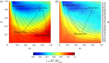
space is shown in figure 5. We define a dimensionless parameter,
 $$\begin{eqnarray}\unicode[STIX]{x1D716}=\overline{Fr}^{\ast }/\overline{Fr}_{\unicode[STIX]{x1D719}=0}^{\ast },\end{eqnarray}$$
where
 $\overline{Fr}_{\unicode[STIX]{x1D719}=0}^{\ast }$
is the base value from the flat-bed case. Hence, figure 5 represents the net effects of the array with a specific
 $\unicode[STIX]{x1D707}_{x}$
–
 $\unicode[STIX]{x1D707}_{y}$
combination on the gravity current’s front propagation with respect to the unobstructed flat-bed condition. By allowing for the independent variation of
 $\unicode[STIX]{x1D707}_{x}$
and
 $\unicode[STIX]{x1D707}_{y}$
with the corresponding
 $\unicode[STIX]{x1D719}$
-contours embedded, figure 5 facilitates a convenient and unambiguous interpretation of the parametric dependence of the various flow regimes on the array geometry. The key message is that there is a wide range of possible states of flow along a single contour of
 $\unicode[STIX]{x1D719}$
, emphasizing the inappropriateness of using the conventional
 $\unicode[STIX]{x1D719}$
-parameterization of array geometry for non-equidistant arrays (
 $\unicode[STIX]{x1D707}_{x}\neq \unicode[STIX]{x1D707}_{y}$
).
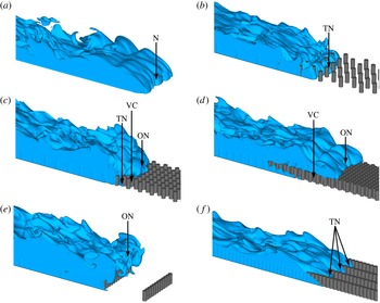
The density structures corresponding to different flow regimes are shown in figure 6. In the flat-bed case F-0 (figure 6
a), the classic gravity current interface and the lobe-and-cleft structures are clearly observed. Once the array of cylinders is present, the flow structure starts to differ from the flat-bed case to varying degrees. Depending on the specific combination of
 $\unicode[STIX]{x1D707}_{x}$
and
 $\unicode[STIX]{x1D707}_{y}$
, four distinct flow regimes of an obstructed gravity current are possible:
Variation of
 $\unicode[STIX]{x1D716}$
using the
 $\unicode[STIX]{x1D707}_{x}$
–
 $\unicode[STIX]{x1D707}_{y}$
space. (a) In-line arrays; (b) staggered arrays. Solid curves indicate contours of
 $\unicode[STIX]{x1D719}=(\unicode[STIX]{x03C0}/4)\unicode[STIX]{x1D707}_{x}\unicode[STIX]{x1D707}_{y}$
with their values marked on the right-hand side of (b). Approximate regions corresponding to different flow regimes are annotated in both panels. Different paths of flow regime change are shown by dashed arrows. The submergence ratio is fixed at
 $H/h=5.4$
.
Visualization of representative flow structures using instantaneous density isosurfaces,
 $\unicode[STIX]{x1D70C}\geqslant 0.5$
. (a) F-0 (unobstructed flat bed,
 $\unicode[STIX]{x1D719}=0$
); (b) S-0.363-0.363 (equidistant and sparse,
 $\unicode[STIX]{x1D719}=0.103$
); (c) S-0.636-0.636 (equidistant and dense,
 $\unicode[STIX]{x1D719}=0.318$
); (d) S-1.000-1.000 (highest density achievable for circular cylinders,
 $\unicode[STIX]{x1D719}=\unicode[STIX]{x03C0}/4$
); (
 $e$
) I-0.090-1.000 (impermeable fences,
 $\unicode[STIX]{x1D719}=0.071$
); (
 $f$
) I-1.000-0.272 (channelization,
 $\unicode[STIX]{x1D719}=0.214$
). The arrows mark the unobstructed nose (N), through-nose within the array (TN), over-nose above the array (ON) and the vertical convection within the pore regions (VC), respectively.

-
(i) Through-flow (figure 6 b). For in-line arrays with small
$\unicode[STIX]{x1D707}_{x}$
and small
$\unicode[STIX]{x1D707}_{y}$
or staggered arrays with arbitrary
$\unicode[STIX]{x1D707}_{x}$
and small
$\unicode[STIX]{x1D707}_{y}$
, the gravity current propagates along the channel bed, finding its way through the regions between individual obstacles, which is referred to as the through-nose (TN). The isolated cylinder wakes and their interferences act as the major turbulence energy dissipator (Cenedese et al.
Reference Cenedese, Nokes and Hyatt2016). This regime bears some similarities to gravity currents in sparse emergent canopies (Tanino et al.
Reference Tanino, Nepf and Kulis2005) or gravity currents propagating inside a highly porous medium over a solid boundary (Ozan et al.
Reference Ozan, Constantinescu and Hogg2015) where the current interface resembles that of a classic flat-bed gravity current (figure 6
a). -
(ii) Over-flow (figure 6 c,d). For arrays with large
$\unicode[STIX]{x1D707}_{x}$
and large
$\unicode[STIX]{x1D707}_{y}$
, due to the excessive drag of a dense array with respect to the horizontal pressure gradient, a well-defined over-nose (ON) propagates along the top boundary of the array and controls the overall current propagation. Significant vertical convection (VC) occurs between the over-nose and the underlying lighter ambient fluid, leading to intense turbulent mixing (Cenedese et al.
Reference Cenedese, Nokes and Hyatt2016). The volume of dense fluid trapped within the array increases with propagated distance of the current. Therefore, the advancement of the over-current is accompanied by a continuous loss of the effective buoyancy that drives its propagation, which scales as (4.2)where
$$\begin{eqnarray}{\mathcal{B}}_{e}\sim g_{e}^{\prime }{\mathcal{V}}_{e},\end{eqnarray}$$
$g_{e}^{\prime }$
is the effective reduced gravity of the gradually diluted over-nose (
$g_{e}^{\prime }\leqslant g_{e,t=0}^{\prime }=g(\unicode[STIX]{x1D70C}_{max}-\unicode[STIX]{x1D70C}_{min})/\unicode[STIX]{x1D70C}_{max}$
), and
${\mathcal{V}}_{e}$
is the gradually reduced volume of dense fluid above the array top boundary (
${\mathcal{V}}_{e}\leqslant {\mathcal{V}}_{e,t=0}=WL_{lock}(H-h)$
), using the notation in figure 1. This buoyancy loss is balanced by the reinjection of dense fluid from the current tail. The over-flow regime is similar to gravity currents over a porous boundary (Ungarish & Huppert Reference Ungarish and Huppert2000) or particle-driven gravity currents (An et al.
Reference An, Julien and Venayagamoorthy2012) in the sense that the dense current system undergoes a continuous loss of effective buoyancy as it advances. The through-current, albeit weakened, still persists (figure 6
c) until the maximum array density for circular cylinders (
$\unicode[STIX]{x1D719}=\unicode[STIX]{x03C0}/4\approx 0.785$
) is achieved where no longitudinal propagation is permitted within the array (figure 6
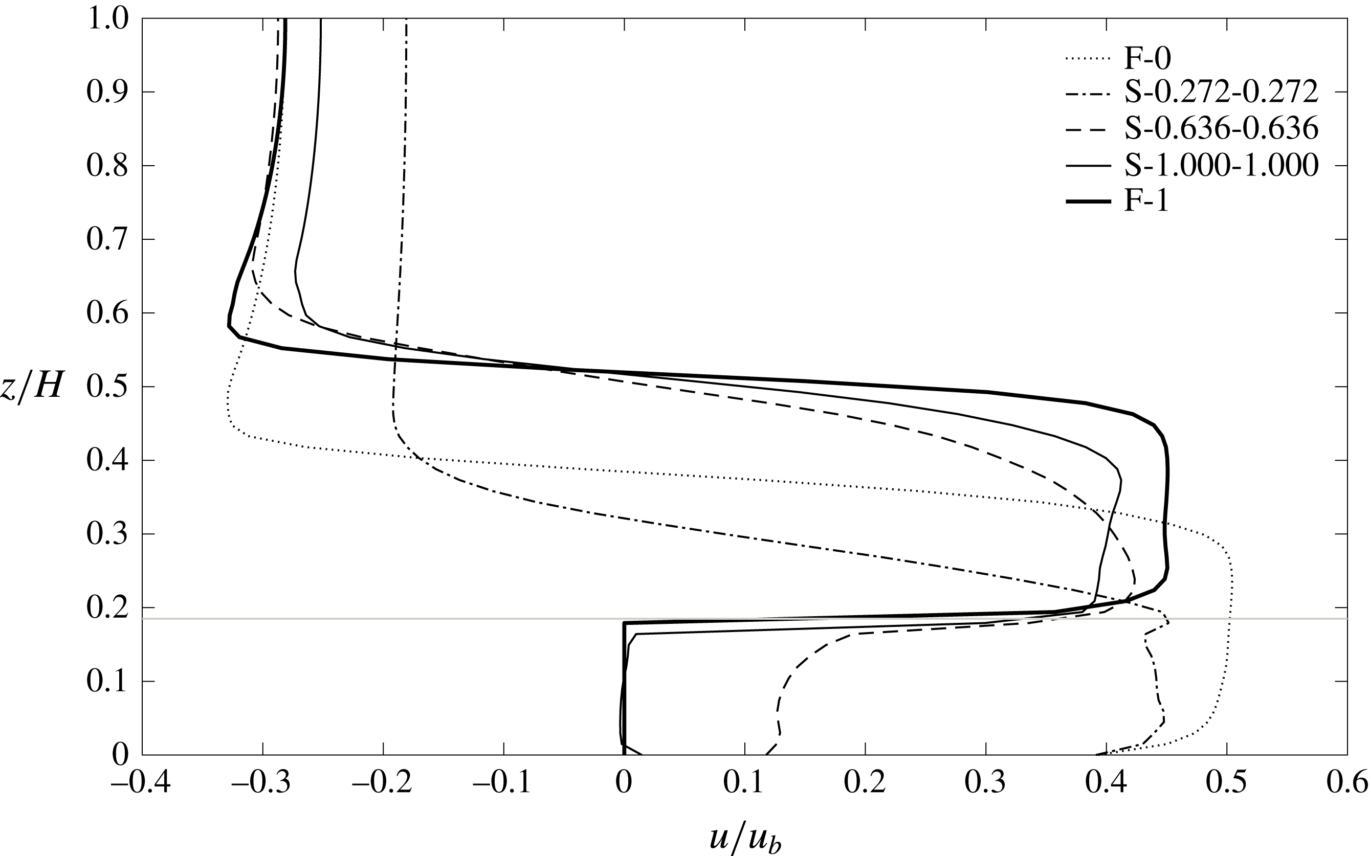
d). This is also evident in the horizontal velocity profiles in figure 8. In the latter case, the fluid motion within the pores is purely convective, and the shape of the over-nose evolves closer to the flat-bed limit.
-
(iii) Plunging-flow (figure 6 e). For arrays with small
$\unicode[STIX]{x1D707}_{x}$
and large
$\unicode[STIX]{x1D707}_{y}$
, the non-equi distant array (
$\unicode[STIX]{x1D707}_{x}\neq \unicode[STIX]{x1D707}_{y}$
) greatly affects the current propagation dynamics. Due to the strong blocking effect by each spanwise row of obstacles, the nose of the gravity current propagates upwards when it reaches the upstream face of each spanwise row, and then plunges towards the bed between two adjacent rows. This is similar to the
$k$
-type roughness reviewed by Jimenez (Reference Jimenez2004) for constant-density flows. The large eddy simulations of a gravity current over a series of submerged two-dimensional obstacles by Tokyay et al. (Reference Tokyay, Constantinescu and Meiburg2011) fall within this category. -
(iv) Skimming-flow (figure 6 f). For in-line arrays with large
$\unicode[STIX]{x1D707}_{x}$
and small
$\unicode[STIX]{x1D707}_{y}$
, the cylinder wakes are greatly suppressed, and the gravity current is separated into several highly independent subcurrents that propagate through the array interior along the streamwise direction, with minimal cross-stream interactions. Here, we follow the nomenclature of Oke (Reference Oke1988) where the mesoscale atmospheric boundary-layer flow is almost decoupled from the recirculation region within urban canopies when buildings are closely spaced, corresponding to the
$d$
-type roughness in Jimenez (Reference Jimenez2004), if applied to the spanwise direction. This is the only regime that is absent in staggered arrays where streamwise channelizing is always interrupted by the next offset rows (compare figure 5
a,b).








In figure 5, starting from the flat-bed case (lower left hand corner) and moving along the
 $45^{\circ }$
-diagonal (equidistant arrays),
 $\unicode[STIX]{x1D716}$
is seen to first decrease and then increase at very large
 $\unicode[STIX]{x1D707}_{x}$
and
 $\unicode[STIX]{x1D707}_{y}$
due to the through-over flow regime change. However, when moving along the detours of the through-plunging (skimming)-over flow regime change, the non-equidistance of the array significantly influences the flow dynamics. In the plunging-flow regime the current propagation can be heavily impeded by arrays with very small
 $\unicode[STIX]{x1D719}$
, whereas in the skimming-flow regime the gravity current may be propagating even faster than in the flat-bed case for in-line arrays (i.e.
 $\unicode[STIX]{x1D716}>1$
, note the scale of colour bar in figure 5). The three pathways of flow regime change, i.e. the through-over, through-plunging-over and through-skimming-over, will be discussed in detail in § 5.
The most remarkable difference between the in-line and staggered cylinder arrangements is the non-existence of the skimming-flow regime in the latter (figure 5
b) due to the cylinder’s offset flow interruption. The blue zone with low values of
 $\unicode[STIX]{x1D716}$
in figure 5(b) appears more diffused than that in figure 5(a). This can be explained using the one-dimensional plots shown in figure 4 where either of the two parameters,
 $\unicode[STIX]{x1D707}_{x}$
and
 $\unicode[STIX]{x1D707}_{y}$
, is fixed as follows. (i) Streamwise densification: in figure 4(c), except along contours of very large
 $\unicode[STIX]{x1D707}_{y}$
, the increase of
 $\unicode[STIX]{x1D707}_{x}$
is accompanied by a decrease of
 $\overline{Fr}^{\ast }$
, signifying a net increase of resistance to the through-current as opposed to the case of in-line arrays (figure 4
a). This extends the zone of low
 $\unicode[STIX]{x1D716}$
to the lower right portion of figure 5(b); and (ii) spanwise densification: in figure 4(d),
 $\overline{Fr}^{\ast }$
starts to increase at smaller value of
 $\unicode[STIX]{x1D707}_{y}$
along contours of larger
 $\unicode[STIX]{x1D707}_{x}$
, signifying an earlier change to the over-flow as compared to the almost unchanged threshold value of
 $\unicode[STIX]{x1D707}_{y}$
in figure 4(b). This causes a less prominent deep-blue zone in the upper right portion of figure 5(b).
5 Change of flow regimes
In what follows, we discuss the three possible paths of flow regime change annotated by the dashed arrows in figure 5.
5.1 Equidistant array: through-over regime change
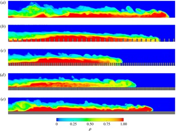
Instantaneous fluid density fields along the channel centreline at
 $t=21.5t_{0}$
showing the
 $T\Rightarrow O$
regime change. (a) F-0; (b) S-0.272-0.272; (c) S-0.636-0.636; (d) S-1.000-1.000; (
 $e$
) F-1. Roughness elements are shown in dark grey. The lock region (
 $-L_{lock}\leqslant x<0$
) is not shown.

In this section, we analyse the dynamics of flow regime change from the through-flow to the over-flow (
 $T\Rightarrow O$
) for equidistant arrays. Figure 7 depicts the instantaneous fluid density fields with
 $\unicode[STIX]{x1D719}$
ranging from 0 to 1. Figure 7(a) shows the classic structure of a gravity current propagating on a smooth bottom. In figure 7(b), the array is sparse such that the gravity current propagates along the channel bed, finding its way either between or over the cylinders. Compared with the flat-bed case, the net increase of array drag slows down the gravity current mainly by the turbulent dissipation in the cylinder wakes. Denser arrays tend to divert the current above the array, and a discernible over-current gradually emerges (figure 7
c). The over-current is diluted mainly by the vertical convection between the over-current and the lighter ambient fluid underneath. In case S-1.000-1.000 (figure 7
d), the through-flow is completely blocked and the current fills the space between cylinders with dense fluid as it advances. The vertical convection is stronger and thus enhances the current dilution as compared with that in figure 7(c). Finally, in the solid-slab case (figure 7
e), the dense fluid only exists and propagates above the solid slab with a height
 $h$
placed on the channel bed. The density structure again resembles that of the flat-bed case but with a smaller flow depth,
 $H-h$
.
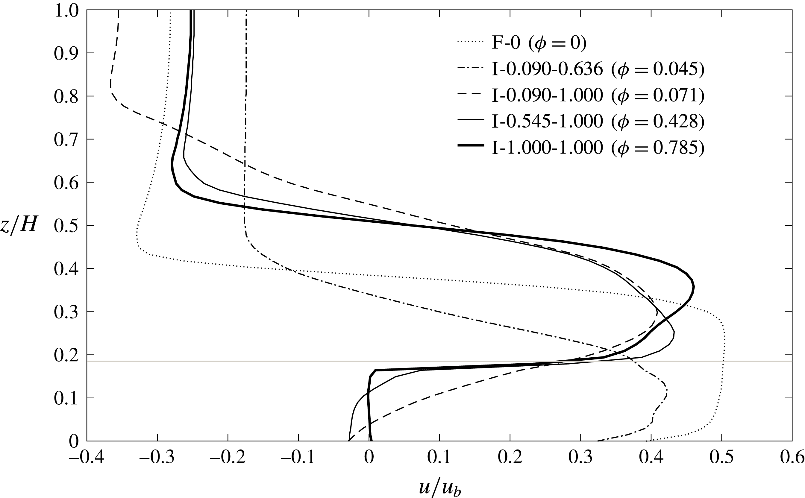
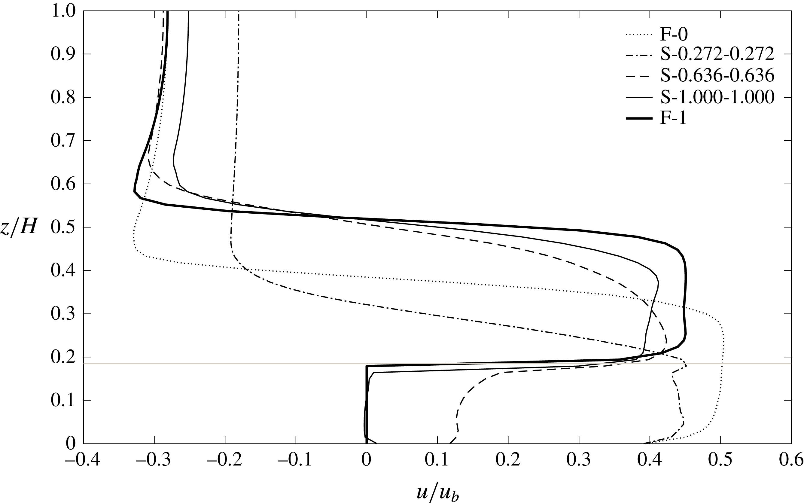
Time-averaged and laterally averaged horizontal velocity profiles showing the
 $T\Rightarrow O$
regime change. The velocity data are recorded at a distance of
 $H/2$
behind the current nose by moving with the gravity current’s front frame. The horizontal grey line marks the array top.
Instantaneous density isosurface at
 $\unicode[STIX]{x1D70C}=0.5$
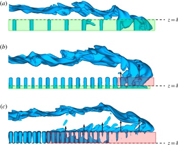
for different array densities. (a) S-0.272-0.272; (b) S-0.636-0.636; (c) S-1.000-1.000. The horizontal dashed lines roughly divide the array region into a longitudinal propagation zone (
 $0\leqslant z<\unicode[STIX]{x1D6FF}$
, encompassed by the green window) and a vertical convection zone (
 $\unicode[STIX]{x1D6FF}\leqslant z<h$
, encompassed by the red window). Arrows indicate the ejection of the lighter ambient fluid from underneath, with their length signifying the strength of the vertical exchange. Note, the vertical convection is more pronounced near the over-nose, and vanishes far upstream where the water column within the array is largely homogenized.

It is evident from figures 5 and 7 that the time-averaged front velocity of the gravity current increases for the over-flow regime compared to the through-flow regime as the array density is increased. This
 $T\Rightarrow O$
regime change is the first mechanism for increasing
 $\overline{Fr}^{\ast }$
for a gravity current past a submerged array. For this path of regime change, the pore regions between the cylinders behave like a ‘void roughness’ in the sense that the over-current is subject to less momentum loss as it approaches the solid-slab limit F-1 with a porosity
 $p=0$
(i.e.
 $\unicode[STIX]{x1D719}=1$
). In case F-1, according to equation (4.2),
 ${\mathcal{V}}_{e}\equiv {\mathcal{V}}_{e,t=0}$
since no trapping of dense fluid within the array occurs after the gate removal. Assuming negligible effects of the abrupt elevation of the channel bottom at the lock gate, an estimate of the Froude number can be obtained as
 $$\begin{eqnarray}\overline{Fr}_{\unicode[STIX]{x1D719}=1}^{\ast }=\overline{Fr}_{\unicode[STIX]{x1D719}=0}^{\ast }\sqrt{\frac{H-h}{H}},\end{eqnarray}$$
where
 $H-h$
is the effective lock height. The resulting
 $\overline{Fr}_{\unicode[STIX]{x1D719}=1}^{\ast }$
for
 $H/h=5.4$
is calculated to be 0.406 (
 $\unicode[STIX]{x1D716}=90\,\%$
), which is slightly larger than the LES value of 0.401 (
 $\unicode[STIX]{x1D716}=89\,\%$
), presumably because of the energy loss near the leading edge of the slab at
 $x=0$
. For case S-1.000-1.000,
 $\overline{Fr}_{\unicode[STIX]{x1D719}=\unicode[STIX]{x03C0}/4}^{\ast }=0.363$
(
 $\unicode[STIX]{x1D716}=81\,\%$
). This reduction in Froude number can be explained by the presence of the pores between cylinders which results in a reduction of
 ${\mathcal{V}}_{e}$
. In addition, the effective density difference,
 $g_{e}^{\prime }$
, is also reduced due to the enhanced dilution of the over-current with respect to the solid-slab case. Consequently, the reduction of
 ${\mathcal{B}}_{e}$
that is absent in the solid-slab case results in a
 $9.5\,\%$
difference between
 $\overline{Fr}_{\unicode[STIX]{x1D719}=\unicode[STIX]{x03C0}/4}^{\ast }$
and
 $\overline{Fr}_{\unicode[STIX]{x1D719}=1}^{\ast }$
.
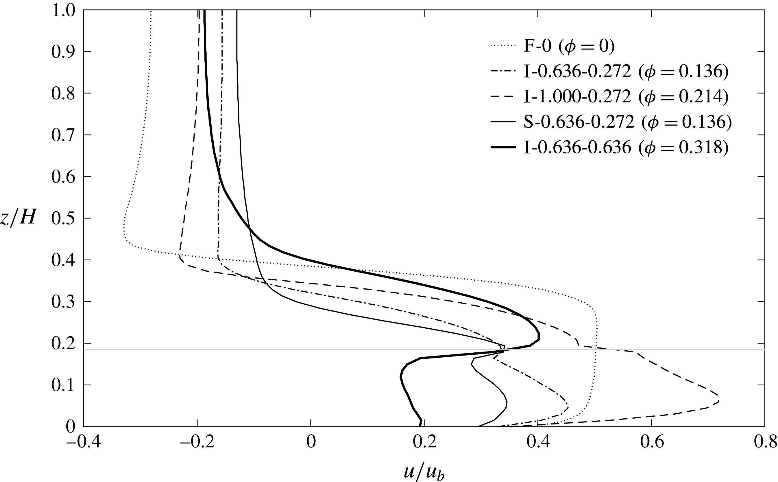
Figure 8 shows the time-averaged and laterally averaged horizontal velocity profiles in the slumping phase corresponding to the cases in figure 7. Starting from the flat-bed case, a clear change from through-flow regime to over-flow regime can be observed. The velocity profile of the through-flow case, S-0.272-0.272, resembles that of case F-0 but with smaller mean magnitude. As
 $\unicode[STIX]{x1D719}$
increases further, the average horizontal velocity within the array decreases, and reaches zero in cases S-1.000-1.000 and F-1 as expected, which implies a gradual suppression of longitudinal propagation. Meanwhile, above the array, the horizontal momentum of the over-current increases as the array is densified, and eventually reaches the solid-slab case where all the dense fluid is propagating along the array top.
The array density
 $\unicode[STIX]{x1D719}$
is observed to influence the driving mechanism of the flow within the array, which is similar to that of constant-density barotropic flows over a submerged canopy despite the difference in flow forcing. For example, Nepf (Reference Nepf2012) suggested that for a sparse array, the velocity follows a turbulent boundary-layer profile, while for a dense array, suppression of the downward penetration of the vertical turbulent stress leads to enhanced shear below and above the array top. Similarly, in the context of gravity currents, for sparse arrays, the velocity follows a hyperbolic-tangent profile as with the classic flat-bed case (compare velocity profiles of F-0 and S-0.272-0.272 in figure 8). As the array becomes denser, there is a gradual suppression of through-current propagation and increase of velocity of the over-current, which strengthens the horizontal shear layer at the array top boundary.
Figure 9 sheds some light on the dilution of the over-current observed in figure 7. We define the lower region of the array as the ‘longitudinal propagation zone’ (
 $0\leqslant z<\unicode[STIX]{x1D6FF}$
) where the flow communicates with the surrounding water predominantly through longitudinal current propagation. The remaining upper array is defined as the ‘vertical convection zone’ (
 $\unicode[STIX]{x1D6FF}\leqslant z<h$
) where turbulent buoyancy fluxes dominate the flow behaviour. The vertical convection zone (if it exists) is only prominent near the over-nose, and weakens upstream of the nose due to the gradual homogenization of the water column within the array after the passage of the over-current. In figure 9(a), the gravity current is in the through-flow regime and no vertical convection zone exists. The in-array flow is purely due to longitudinal advection driven by the pressure gradient. In figure 9(b), the increase of array drag results in the coexistence of over- and through-currents interconnected by a vertical convection zone. One portion of the lighter fluid between the cylinders is vertically exchanged with the denser over-current, while the remaining favours a horizontal propagation below
 $z=\unicode[STIX]{x1D6FF}$
, forming the longitudinal propagation zone. However, for the case in which horizontal propagation is completely blocked (figure 9
c), despite the smaller amount of lighter fluid initially within the array at higher
 $\unicode[STIX]{x1D719}$
, it is all forced to exchange with the overlying denser over-current, resulting in an enhanced dilution of the over-current as shown in figure 7(d) in comparison with that in figure 7(c).
5.2 Non-equidistant array
We discuss in this section under what circumstances the
 $\unicode[STIX]{x1D707}_{x}$
–
 $\unicode[STIX]{x1D707}_{y}$
characterization is necessary. As indicated in figure 5, in addition to a direct change from through-flow to over-flow, there are two other possible detours that lead to the same destination.
5.2.1 Through-skimming-over regime change
Instantaneous fluid density fields at
 $t=21.5t_{0}$
showing the
 $T\Rightarrow S\Rightarrow O$
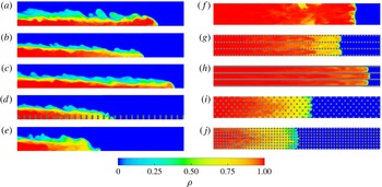
regime change. (a,f) F-0; (b,g) I-0.636-0.272; (c,h) I-1.000-0.272; (d,i) S-0.636-0.272; (e,j) I-0.636-0.636. The left panels are plotted in the
 $x$
–
 $z$
plane along the array centreline, and the right panels are plotted in the
 $x$
–
 $y$
plane located
 $0.2h$
above the channel bed. Roughness elements are shown in dark grey. Note that in (d) the centreline density data are not available at every other cylinder in the streamwise direction due to the staggered arrangement.

Time-averaged and laterally averaged horizontal velocity profiles showing the
 $T\Rightarrow S\Rightarrow O$
regime change. The velocity data are recorded at a distance of
 $H/2$
behind the current nose by moving with the gravity current’s front frame. The horizontal grey line marks the array top.

The through-skimming regime change is another mechanism for increasing the
 $\overline{Fr}^{\ast }$
of the gravity current other than the through-over regime change. Figures 10 and 11 show the density and velocity structures during the through-skimming-over regime change, respectively. It is obvious that the information provided by the array density
 $\unicode[STIX]{x1D719}$
about the current propagation for non-equidistant arrays is fairly misleading. For case I-0.636-0.272 (figure 10
b,g), all the cylinders are subject to strong wake interferences due to their streamwise closeness. Three discernible subcurrents can be observed but with enhanced dilution with respect to the flat-bed case, due to the still persisting wake-induced mixing. The current is within an intermediate regime between through-flow and skimming-flow where cross-stream interaction between subcurrents is weak but non-negligible. The wake sheltering effect results in a significant drop of form drag per cylinder upon the incoming flow with this specific configuration. Therefore, when moving along the contour of
 $\unicode[STIX]{x1D719}=0.136$
in figure 5(a), the current in case I-0.636-0.272 has a much larger
 $\unicode[STIX]{x1D716}$
as compared to other array configurations with the same array density. As
 $\unicode[STIX]{x1D707}_{x}$
increases to 1 (figure 10
c,h), the cylinder wakes have been completely suppressed and the array has been fully channelized. The three subcurrents only communicate with each other in the above-array area (
 $z>h$
), and thus a sudden contraction of the channel cross-sectional area below
 $z=h$
increases the front velocity due to conservation of mass. The current in this particular configuration propagates faster than in the flat-bed case, as shown in figure 11, resulting in the larger values of
 $\unicode[STIX]{x1D716}$
in the lower right-hand corner of figure 5(a). This is a phenomenon similar to the skimming flows observed in wind passing building clusters (Oke Reference Oke1988), as well as the
 $d$
-type roughness in turbulent flows over rough walls (Jimenez Reference Jimenez2004), where the main streams are separated from the smaller-scale flows within the closely packed roughness elements.
The
 $T\Rightarrow S$
regime change is exclusive for in-line arrangements, and thus there is no skimming-flow regime in figure 5(b). In a staggered array (figure 10
d,i), the high-velocity interstitial flow between the spanwise gaps is always obstructed by the offset rows immediately downstream such that the channelizing is heavily interrupted. Comparison between cases I-0.636-0.272 and S-0.636-0.272 indicates that the difference in cylinder arrangement alone may result in a significant change of the gravity current propagation dynamics for arrays with high values of
 $\unicode[STIX]{x1D707}_{x}/\unicode[STIX]{x1D707}_{y}$
.
Along the contours of
 $\unicode[STIX]{x1D707}_{x}=1$
in figure 4(b), the value of
 $\overline{Fr}^{\ast }$
first increases beyond the flat-bed limit and peaks around
 $\unicode[STIX]{x1D707}_{y}=0.25$
. Further increase of
 $\unicode[STIX]{x1D707}_{y}$
results in a considerable increase of array drag such that the gravity current is unable to squeeze into the subchannels. The increase of
 $\overline{Fr}^{\ast }$
due to the
 $T\Rightarrow S$
regime change is compensated by a significant reduction of flow rate, and thus
 $\overline{Fr}^{\ast }$
starts to decrease. In figure 11, the velocity profile of case I-0.636-0.636 indicates that the current is changing from the skimming-flow to over-flow regime due to the increase of
 $\unicode[STIX]{x1D707}_{y}$
when compared with case I-0.636-0.272. With even larger
 $\unicode[STIX]{x1D707}_{y}$
(see figure 4
b), the current completely changes to the over-flow regime, during which
 $\overline{Fr}^{\ast }$
increases again.
Instantaneous fluid density fields along the channel centreline at
 $t=21.5t_{0}$
showing the
 $T\Rightarrow P\Rightarrow O$
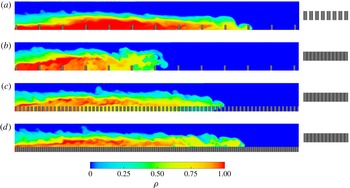
regime change. (a) I-0.090-0.636; (b) I-0.090-1.000; (c) I-0.545-1.000; (d) I-1.000-1.000. Frontal cylinder configurations as seen by the current are shown on the right.

Time-averaged and laterally averaged horizontal velocity profiles showing the
 $T\Rightarrow P\Rightarrow O$
regime change. The velocity data are recorded at a distance of
 $H/2$
behind the current nose by moving with the gravity current’s front frame. The horizontal grey line marks the array top.

5.2.2 Through-plunging-over regime change
In this section, we discuss the third path of change of flow regime depicted in figure 5, focusing on the configurations with large
 $\unicode[STIX]{x1D707}_{y}$
. Again, relevant density fields and velocity profiles are shown in figures 12 and 13, respectively. According to figure 12(a), case I-0.090-0.636 is within the through-flow regime where the gravity current mainly propagates between the cylinders. The values of
 $\unicode[STIX]{x1D707}_{y}$
for the remaining cases are all unity for each row of cylinders to be felt as impermeable by the current, based on which we assess the effect of streamwise array densification. Keeping
 $\unicode[STIX]{x1D707}_{x}=0.090$
, as
 $\unicode[STIX]{x1D707}_{y}$
is increased to 1 (figure 12
b), the current is right within the plunging-flow regime and its propagation is greatly impeded. For all the simulation cases shown, the streamwise spacing between the cylinders, if normalized by the water depth
 $H$
, is comparable or small with respect to the vertical dimension of the current due to the deep submergence of the array. Therefore, even with
 $\unicode[STIX]{x1D707}_{x}$
as low as 0.090, the corresponding velocity profile in figure 13 indicates that the contact time of the current nose with the channel bed is very limited. Time history of the current propagation (not shown) indicates that after the nose reattaches to the bed, it hardly favours a horizontal propagation but rather begins to climb the next row of cylinders. The gravity current undergoes significant mixing and energy dissipation during these climbing and plunging motions. We expect more contact of the current nose with the channel bed as the submergence ratio
 $H/h$
decreases. Consistent with figure 4, the change of regime from plunging-flow to the over-flow occurs immediately after
 $\unicode[STIX]{x1D707}_{x}$
is increased beyond 0.090. Along the path of the through-plunging-over flow regime change, the gravity current is first greatly impeded by the
 $T\Rightarrow P$
regime change, reaching the region with lowest
 $\unicode[STIX]{x1D716}$
in figure 5, and then
 $\overline{Fr}^{\ast }$
increases again because of the
 $P\Rightarrow O$
regime change.
6 Summary and conclusions
Submerged canopies are ubiquitous in aquatic flows and even more commonly seen in oceanic and atmospheric environments. Laboratory experiments and large eddy simulations were used to study lock-exchange gravity currents propagating over and through an array of submerged circular cylinders. Laboratory and numerical results were observed to be in excellent agreement and the parameter space of the numerical simulations was extended to cover a much wider range of array geometries (over 200 numerical simulations), in order to provide a comprehensive understanding of the influences of array density (
 $\unicode[STIX]{x1D719}$
) and non-equidistance (
 $\unicode[STIX]{x1D707}_{x}\neq \unicode[STIX]{x1D707}_{y}$
) that have not been adequately addressed by previous studies.
In order to investigate the behaviour of the gravity current (e.g. the front velocity) over the whole range of
 $\unicode[STIX]{x1D719}$
, the array density was varied from the unobstructed flat-bed case (
 $\unicode[STIX]{x1D719}=0$
) towards the solid-slab case (
 $\unicode[STIX]{x1D719}=1$
). When a gravity current encounters a dense array submerged in the fluid (
 $H/h>1$
) with excessive drag, the existence of the additional flow pathway outside the array brings about the fundamental difference in current propagation compared with that of an emergent array. Starting from the flat-bed case, the time-averaged Froude number
 $\overline{Fr}$
was initially seen to decrease as
 $\unicode[STIX]{x1D719}$
increases, which is consistent with current propagation in emergent canopies. However, as
 $\unicode[STIX]{x1D719}$
increases further, our experiments indicated for the first time a non-monotonic dependence of
 $\overline{Fr}$
on
 $\unicode[STIX]{x1D719}$
which was confirmed by the numerical simulations (figure 3). As the array gradually approaches a solid slab, the diminishing individual cylinder wakes together with the smaller amount of dense fluid trapped within the pore regions, jointly result in a smaller momentum loss of the over-current. This through-over flow regime change associated with the densification of an equidistant array was observed to be the first mechanism for increasing the front speed of a gravity current as
 $\unicode[STIX]{x1D719}$
increases (figures 7 and 8).
Strictly speaking, it is rare that an array is absolutely equidistant. When
 $\unicode[STIX]{x1D707}_{x}\approx \unicode[STIX]{x1D707}_{y}$
, the conventional array characterization, which uses the horizontally averaged parameter
 $\unicode[STIX]{x1D719}$
, can be applied with acceptable error. However, for a gravity current encountering a highly non-equidistant array, we have shown that the flow condition cannot be uniquely determined by
 $\unicode[STIX]{x1D719}$
alone. Instead, its orthogonal components are individually important. Consequently, we proposed a new geometrical framework consisting of the streamwise and spanwise array densities,
 $\unicode[STIX]{x1D707}_{x}$
and
 $\unicode[STIX]{x1D707}_{y}$
, to provide a more convenient and unambiguous prediction of the gravity current propagation for highly organized but non-equidistant arrays. Physically,
 $\unicode[STIX]{x1D707}_{x}$
controls the wake sheltering and
 $\unicode[STIX]{x1D707}_{y}$
controls the current intrusion. It is argued that a wide range of flow conditions are possible along a single contour of
 $\unicode[STIX]{x1D719}$
in figure 5, emphasizing the breakdown of the
 $\unicode[STIX]{x1D719}$
-parameterization.
Depending on the specific
 $\unicode[STIX]{x1D707}_{x}$
–
 $\unicode[STIX]{x1D707}_{y}$
combination, four dynamically different flow regimes are identified. The flow falls into the through-flow regime with small
 $\unicode[STIX]{x1D707}_{x}$
and small
 $\unicode[STIX]{x1D707}_{y}$
for in-line arrays (figure 5
a), or arbitrary
 $\unicode[STIX]{x1D707}_{x}$
and small
 $\unicode[STIX]{x1D707}_{y}$
for staggered arrays (figure 5
b), where the gravity current propagates along the bed and is influenced by strong cylinder wakes. For sufficiently large
 $\unicode[STIX]{x1D707}_{x}$
and
 $\unicode[STIX]{x1D707}_{y}$
, a well-defined over-current emerges and rides on the array top (i.e. over-flow regime) irrespective of the cylinder arrangement. As one moves away from the lower left to upper right
 $45^{\circ }$
-diagonal (i.e., increasing array non-equidistance) in figure 5(a), two extreme conditions can occur: (i) in the energy-consuming plunging-flow regime (small
 $\unicode[STIX]{x1D707}_{x}$
and large
 $\unicode[STIX]{x1D707}_{y}$
), the gravity current propagates upwards over the row of cylinders and then plunges towards the bed between two adjacent rows; and (ii) for the skimming-flow exclusively occurring for in-line arrays with large
 $\unicode[STIX]{x1D707}_{x}$
and small
 $\unicode[STIX]{x1D707}_{y}$
, the high-speed channelized gravity currents may even propagate faster than in the flat-bed case due to the abrupt contraction of the flow cross section within the array. This through-skimming flow regime change is identified as the second mechanism for increasing the front speed of a gravity current as
 $\unicode[STIX]{x1D719}$
increases. It is absent for staggered arrays with offset interruption (figures 10 and 11), highlighting the effect of cylinder arrangement pattern (note the difference between figures 5
a and 5
b).
Hydrologic storage occurs in regions of diminished flow in which water can remain in contact with biologically and geochemically active surfaces for an extended time before moving downstream (Harvey, Conklin & Koelsch Reference Harvey, Conklin and Koelsch2003). Longer periods of hydrologic retention in submerged canopies contributes to the nutrient removal for water quality applications, and more broadly, to hydrologic storage (Nepf et al. Reference Nepf, Ghisalberti, White and Murphy2007). However, the true retention time associated with dense partial-depth canopies in field conditions is often much shorter than what is estimated based on the through-current propagation (Ozan et al. Reference Ozan, Constantinescu and Nepf2016). The possible explanation is that as the array becomes denser, the front speed of the over-current gradually increases and overtakes the underlying through-current (figure 8). As a result, the water renewal in the canopy region downstream of the through-current is mainly accomplished by vertical exchange due to the unstable stratification between the dense over-current and the lighter fluid within the array (figure 9). This increased canopy flushing rate prevents the nutrient uptake of the submerged vegetation from being supply-limited, partly compensating the declined growth rate caused by the weakened longitudinal transport of nutrients within a dense array. In this regard, the effect of the through-over flow regime change on the retention time in submerged canopies is a key part of our understanding of how fluid mechanics influences the ecology of lotic ecosystems.
The fast spreading destructive gravity current flows (e.g. snow avalanches, haboobs and pyroclastic flows) pose a significant threat to lives and properties. Hence there is a critical need for effective preventative measures to mitigate their impact. The region with the smallest front velocities (plunging-flow) in figure 5 well explains the fact that snow fences are always built perpendicular to the mountain slope. Since a very early change of regime to over-flow is possible for an array with large
 $\unicode[STIX]{x1D707}_{y}$
(figure 4
c), special attention should be paid to the gaps between rows to prevent unexpectedly high approaching speed of the avalanche due to the plunging-over flow regime change (figures 12 and 13). Meanwhile, in urban canopies where the buildings may be highly channelized, the inclusion of the directional information of atmospheric gravity fronts (e.g. haboobs and sea breezes) in weather forecasting models is necessary. These propagating fronts may be heavily impeded if their path is perpendicular to the streets (plunging-flow), or on the contrary, expedited if they advance along the streets (skimming-flow).
It is noteworthy that not only the array drag, but also the incoming buoyancy forcing (i.e.
 $g^{\prime }$
and
 $H$
), determines the propagating properties of the gravity currents. Although we are aware that the flow regime diagram in figure 5 is only proposed for a particular submergence ratio of
 $H/h=5.4$
, it is conceivable that it can also be applied to other submergence conditions as long as the array is submerged. However, the boundary between different regimes would require some modifications. For example, figure 3 indicates that a larger submergence ratio tends to increase the Froude number of the gravity currents for a fixed array density. We also expect a deeper submergence to promote the change to over-flow regime because a larger amount of dense fluid will be forced to propagate over the array. Furthermore, this study only considered the case of a homogeneous ambient environment and a particular cylinder aspect ratio
 $h/d$
. A future direction of study will be to investigate how the ambient stratification and variation of
 $h/d$
modify the gravity current propagation.
Acknowledgements
The authors are grateful to the three anonymous referees for their constructive comments and recommendations. The authors would like to thank I. Sheppard and K. Wines for their invaluable technical expertise in constructing the experimental apparatus at the University of Canterbury. S.K.V. and J.Z. gratefully acknowledge the support of both the National Science Foundation under CAREER grant OCE-1151838 and the Office of Naval Research under grant nos N00014-12-0938 and N00014-16-1-3015. Support to C.C. was given by the National Science Foundation project OCE-1333174. S.K.V. and C.C. were able to forge this collaborative research at the Workshop on the Mathematics of Layers and Interfaces that was held in Oaxaca, Mexico from November 8–13, 2015, and hence would like to thank the workshop organizers and the Banff International Research Station for Mathematical Innovation and Discovery, Canada.