




No CrossRef data available.
EFFICIENT LIKELIHOOD INFERENCE IN NONSTATIONARY UNIVARIATE MODELS
Published online by Cambridge University Press: 05 March 2004
Abstract
Recent literature shows that embedding fractionally integrated time series models with spectral poles at the long-run and/or seasonal frequencies in autoregressive frameworks leads to estimators and test statistics with nonstandard limiting distributions. However, we demonstrate that when embedding such models in a general I(d) framework the resulting estimators and tests regain desirable properties from standard statistical analysis. We show the existence of a local time domain maximum likelihood estimator and its asymptotic normality—and under Gaussianity asymptotic efficiency. The Wald, likelihood ratio, and Lagrange multiplier tests are asymptotically equivalent and chi-squared distributed under local alternatives. With independent and identically distributed Gaussian errors and a scalar parameter, we show that the tests in addition achieve the asymptotic Gaussian power envelope of all invariant unbiased tests; i.e., they are asymptotically uniformly most powerful invariant unbiased against local alternatives. In a Monte Carlo study we document the finite sample superiority of the likelihood ratio test.I am grateful to Bent Jesper Christensen, Niels Haldrup, Pentti Saikkonen (the co-editor), and two anonymous referees for many useful comments and suggestions that significantly improved this paper. This work was done while the author was at the University of Aarhus, Denmark.
Information
- Type
- Research Article
- Information
- Copyright
- © 2004 Cambridge University Press
1. INTRODUCTION
In this paper we consider likelihood based estimation and testing within a wide class of possibly nonstationary models, including but not limited to the seasonal fractionally integrated autoregressive moving average (ARMA) model. In such models, estimators and test statistics are often found to have nonstandard distributional properties. In contrast, we show that by adapting time domain procedures and embedding the models of interest in a general I(d) framework, instead of the autoregressive alternatives typically considered in the literature, estimators and test statistics regain the standard distributions and optimality properties well known from simpler models.
Several versions of the Wald, likelihood ratio (LR), and score or Lagrange multiplier (LM) testing procedures have appeared in the literature on nonstationary models, e.g., when conducting Dickey and Fuller (1979) type tests for a unit root (I(1) against I(0)) or testing stationarity (I(0) against I(1)). For a comprehensive recent survey, see Phillips and Xiao (1998). However, these tests have nonstandard limiting distributions that have to be simulated on a case-by-case basis. Some advances have been made recently toward achieving efficient tests. Locally optimal and point optimal tests have been derived for the stationarity hypothesis (e.g., Saikkonen and Luukkonen, 1993a, 1993b) and for the unit root hypothesis (e.g., Elliott, Rothenberg, and Stock, 1996). However, these tests still have nonstandard distributions, and no uniformity results apply.
What is needed is a class of processes that is more general than the unit root I(1) models and admits the testing of smooth hypotheses in the sense that the properties of the process do not differ substantially if the null hypothesis is changed slightly. One such class is that of fractionally integrated processes. Thus, a process is I(d) (fractionally integrated of order d) if its dth difference is I(0); i.e., yt ∈ I(d) if

where

denotes the indicator function and et ∈ I(0). A process is I(0) if it is covariance stationary and its spectrum is bounded and bounded away from zero at any frequency. Testing H0 : d = 1 in (1) may be seen as an alternative to unit root testing. We show that in a fractional integration framework much more desirable properties can be obtained compared with autoregressive (and possibly seasonal and fractional) unit root models where test statistics have nonstandard distributions (see, e.g., Phillips, 1987; Hylleberg, Engle, Granger, and Yoo, 1990; Sowell, 1990).
Notable exceptions to the nonstandard tests are Robinson (1994) and Tanaka (1999), extending earlier work by Robinson (1991) and Agiakloglou and Newbold (1994), and it is the Robinson (1994) model that we consider further in this paper. Robinson (1994) derives the LM test statistic (of (16) and (23), which follow) in the frequency domain, claiming that it is more suitable for the analysis, and shows that the LM test statistic is asymptotically chi-squared distributed and locally most powerful under Gaussianity. In a simulation study it is found that when the data generating process (DGP) is of the fractional type the finite sample performance of the new test is better than that of existing tests, the opposite being the case when the DGP is of the autoregressive type. Tanaka (1999) considers the fractional unit root model in (1) and shows the existence of a local time domain maximum likelihood estimator (MLE) and derives the LM and Wald tests. Tanaka (1999) shows that the estimator is asymptotically normal and, under invariance conditions, that the tests are locally most powerful and indeed asymptotically uniformly most powerful against one-sided local alternatives. Simulations show that in finite samples the time domain tests are superior to the frequency domain LM test of Robinson (1994) with respect to both size and power. The estimator is also shown to be quite close to its asymptotic distribution, except in the presence of errors with strong positive serial correlation.
The main contributions of the present paper when compared with the previous work of Robinson (1994) are summarized in the following five points. (i) All the results are obtained in the time domain, which is most frequently employed by practitioners, whereas Robinson (1994) favors a frequency domain approach. The derivation of results and statement of assumptions in the time domain require different methods than in the frequency domain. Another reason to consider the time domain is that in some cases the resulting estimators and tests are more easily applied than their frequency domain counterparts. (ii) It is of interest to examine the estimation of the model by maximum likelihood because the estimator is expected to have good properties. Indeed, it is shown that standard asymptotics and efficiency apply, which is a great advantage in applied work. (iii) Whereas Robinson (1994) only considers the LM test, we also consider the Wald and LR tests and show that standard asymptotics apply to all the test statistics. (iv) For the submodels with a scalar parameter and independent and identically distributed (i.i.d.) Gaussian errors, the LM, LR, and Wald tests are shown to be uniformly most powerful (against local alternatives) among all invariant and unbiased tests. (v) In a simulation study based on the well-known fractional unit root model it is shown that the LR test outperforms the LM and Wald tests with respect to both size and power.
Contrary to the present paper, Tanaka (1999) considers only a special case of the full model in Robinson (1994), namely, the fractional unit root model, and conducts an analysis similar to ours. We consider the full model.
The paper proceeds as follows. In Section 2 we set up the model and discuss important special cases. In Section 3 we consider inference with martingale difference errors and derive the properties of the estimator and tests, whereas in Section 4 we allow serially correlated errors. Section 5 presents the results of our Monte Carlo experiments, and Section 6 concludes. All proofs are collected in the Appendix.
2. THE MODEL
Suppose we observe the real-valued stochastic process {yt, t = 1,2,…, n} generated by the linear model

where {xt} is a k × 1 purely deterministic component and {ut} is an unobserved error component. Two leading cases for the deterministic terms are xt = 1 and xt = (1, t)′, which yield the models yt = β0 + ut and yt = β0 + β1 t + ut, respectively, but other terms such as seasonal dummies are also allowed for; cf. Assumption 2, which follows. The unobserved error process {ut} is assumed to have the generating mechanism

Here, {et} is a stationary and invertible process with only weakly dependent errors (i.e., no long memory or nonstationarity) and φ(z, θ) is a function of the complex variate z and the p × 1 parameter vector

. The chosen parametrization is such that θ = 0 is the true value, without loss of generality, and this belongs to the interior of Θ.
The model is further required to satisfy the following assumptions.
Assumption 1. The function φ(z, θ) is such that (i) φ(0, θ) = 1 and φ(z, θ) = φ(z) if and only if θ = 0, where φ(z) = φ(z, θ)|θ=0. (ii) φ(z, θ) is twice continuously differentiable in θ in an open convex set Θ* containing Θ and

where

is the coefficient on zj in the expansion of ζ(z) = (∂/∂θ)ln φ(z, θ)|θ=0 in powers of z. (iii) The function λ(z, θ) = (φ(z, θ)/φ(z)) × (∂/∂θ)ln φ(z, θ) is continuous in θ at θ = 0 for almost all z such that |z| = 1, and, letting λj(θ) be the coefficient on zj in the expansion of λ(z, θ) in powers of z, in a neighborhood N of size O(n−1/2) of θ = 0,

.
Assumption 2. The k × 1 vector of regressors xt is nonstochastic and such that

is positive definite for n sufficiently large, where

.
Assumption 3. The innovation sequence in (3), {et, t = 0,±1,±2,…}, satisfies

for all t ≥ 1, where

is an increasing sequence of σ-algebrae, and {et2, t = 0,±1,±2,…} is uniformly integrable.
Some comments on the assumptions follow. Assumption 1 is a time domain equivalent of the assumptions made by Robinson (1994) on the parametric model, where (i) ensures identifiability of θ and (ii) and (iii) are smoothness conditions on the parametric model. The unit root process nested in an autoregressive model is (3) with φ(z, θ) = 1 − (1 + θ)z, but in this case the right-hand-side inequality of (4) is not satisfied. Differentiability to any order is easily verified for all of the examples that follow.
Assumption 2 is a very mild multicollinearity condition on the regressors. It does not even require the smallest eigenvalue of Dn to tend to infinity as n → ∞, which is usually required in linear regression models to get consistent estimates of β.
Finally, Assumption 3 ensures that the innovations are such that

are both uniformly integrable martingale difference sequences. This is more general than i.i.d. and in practice not much more restrictive than uncorrelatedness. An implication of this assumption is that

in probability (e.g., Hall and Heyde, 1980, Theorem 2.22), which we will use later. Assumption 3 can be replaced by any other assumption that gives rise to a weak law of large numbers (LLN) for {et2} and a central limit theorem (CLT) in Theorem 3.1, which follows. Thus, we could presumably relax Assumption 3 to accommodate autoregressive conditional heteroskedasticity/generalized autoregressive conditional heteroskedasticity (ARCH/GARCH) type errors (as suggested by an anonymous referee), which are often found in financial data, where our methods are especially applicable due to the large amount of data available (see also Ling and Li, 1997).
A very general model considered by Robinson (1994), and satisfying the preceding assumptions, is

where for each j, θi(j) = θl for some l, and for each l there is at least one j such that θi(j) = θl; i.e., there are up to h singularities in the spectral density of ut and p ≤ h. That is, we do not require that there is a θj for each singularity. For example, the quarterly I(1) hypothesis is given by either one of the functions φ(z, θ) = (1 − z4)1+θ, where we use the same θ for each of the h = 3 spectral singularities, or φ(z, θ) = (1 − z)1+θ1(1 + z)1+θ2(1 + z2)1+θ3, where the integration orders are allowed to be different at different frequencies under the alternative.
The case considered by Tanaka (1999) is the fractional unit root model defined by

In this model ζ(z) = ln(1 − z) and ζj = −j−1 such that Ψ = π2/6. The weak dependence, unit root, and I(2) models nested in a fractional integration framework correspond to (6) with d = 0, d = 1, and d = 2, respectively.
Another important special case of the general model (5) is the cyclical I(d) or generalized fractional autoregressive integrated moving average (ARIMA) model of Gray, Zhang, and Woodward (1989), recently advocated by Chung (1996), Bierens (2001), and Gil-Alana (2001). This model is generated by the function

where λ is the cyclic frequency of interest. Then d = 1 and θ = 0 corresponds to the cyclic/seasonal unit root at frequency λ.
Finally, suppose the m-vector xt is I(dx) and fractionally cointegrated and the cointegrating vector is known a priori from economic theory such that we can treat ut = α′xt as an observed time series (when the cointegration vector is unknown and must be estimated, the results in the present paper do not apply; see Nielsen, 2003). Then the hypothesis H0 : θ = 0 in (6) with d = dx corresponds to the null of no fractional cointegration, and with d = 0 the hypothesis H0 : θ = 0 corresponds to the null of fractional cointegration with I(0) equilibrium errors. A well-known example is the purchasing power parity. Let xt consist of the time t domestic log-price, foreign log-price, and the log exchange rate, respectively, and suppose xt is fractionally integrated of order d. Then the purchasing power parity predicts that α = (−1,1,1)′ should be a cointegrating vector and that the cointegration residuals should be I(0). Imposing α = (−1,1,1)′ on the data, the last implication can be tested as in (6) with d = 0.
The preceding examples illustrate the generality of our approach. To see why standard asymptotics apply, we briefly discuss the data generating mechanism (see also the discussion by Ling and Li, 2001, pp. 739–741). When {ut} is generated by truncation as in (3), it depends only on the shocks starting at time t = 1 and not on shocks starting in the infinite past as would otherwise be the case. Under (3), there are two fundamentally different approaches to allow for nonstationarity that lead to different asymptotic results. Ling and Li (2001) consider the fractional unit root model (6) assuming that d ∈ (−½,½), the stationary region, and allowing unit roots in the autoregressive polynomial a(z). Standard asymptotics is obtained for the fractional difference parameter, but the estimates of the unit roots have nonstandard Dickey–Fuller type distributions. On the other hand, Robinson (1994) and Tanaka (1999) capture the unit root through the fractional difference parameter d and assume that a(z) is stationary. We follow this practice in the present paper. Because no unit root must be estimated in a(z) we avoid the nonsmooth behavior of the model near the unit roots, and this admits standard asymptotics in our setting.
In the subsequent analysis we first consider the case where {et} is a martingale difference sequence, and then we treat the full model in which {et} is allowed to follow an ARMA process.
3. INFERENCE WITH MARTINGALE DIFFERENCE ERRORS
The Gaussian log-likelihood function of (2) and (3) is

apart from constant terms. The asymptotic results derived in this section impose only Assumption 3 on the error process. Gaussianity is not necessary for most of our results and is used only to choose a likelihood function and to show efficiency.
Because only θ is of interest we concentrate out the nuisance parameter (β′, σ2). This does not influence the results, and in fact

is asymptotically uncorrelated with

(see the formula for the information matrix (21), which follows). The concentrated likelihood is

where


and capital letters denote the appropriate matrices of observations; e.g., X is the n × k matrix with xt′ as the tth row. Here, β(θ) and σ2(θ) are functions of θ. They define the estimator

of (β′, σ2). We shall also need

which is the estimator of (β′, σ2) under the true value of θ. Note that β(θ) is just the ordinary least squares estimator in a regression of φ(L, θ)yt on φ(L, θ)xt and σ2(θ) is the usual maximum likelihood variance estimator for the residual process φ(L, θ)(yt − β(θ)′xt).
Note that the estimate of β need not be consistent in our model. One such case occurs when xt = 1 in the fractional unit root model (6) with d = 1. Then

is inconsistent, but this has no influence on inference based on

(see Robinson, 1994; also see the Appendix). In fact, what we need in the proofs is the relation

which follows under Assumption 2 by definition of

.
3.1. Estimation
In this section we show the existence of a local MLE and derive the limiting distribution theory following the approach of Sargan and Bhargava (1983) and Tanaka (1999). In particular, we consider the conditional sum of squared residuals objective function (9).
In the following we find it convenient to consider maximizing

where

. Assume first that we are in a neighborhood of the true value, i.e., that there exists a δ such that

(the existence of δ will be proved shortly). Then we can show the following results.
THEOREM 3.1. Let Assumptions 1–3 be satisfied and let g(θ) be given by (13). Then, under

,
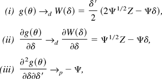
where Z is a p-dimensional standard normal random vector.
Next, we prove the existence of a local MLE

such that

following Sargan and Bhargava (1983) and Tanaka (1999). Let ι be a p × 1 direction vector, i.e., satisfying ∥ι∥ = 1, where ∥·∥ is the Euclidean norm, and let δ = ∥δ∥ι. Generalizing the scalar approach by Sargan and Bhargava (1983) and Tanaka (1999), it suffices to show that
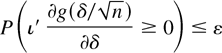
for any direction vector ι, ε > 0, and n ≥ n0 (n0 fixed) and for some ∥δ∥ > 0. Note that

is the directional derivative of g at

, i.e., the rate of change of g at

in the direction ι.
Thus, for all direction vectors ι, moving some distance ∥δ∥ in the direction ι from the true value, the directional derivative of g in the same direction ι should be negative for sufficiently large n. In the one-dimensional case ι = ±1 and (14) reduces to the corresponding conditions of Sargan and Bhargava (1983) and Tanaka (1999). It follows from Theorem 3.1 that

which can be made arbitrarily small by selecting ∥δ∥ large. Thus, (14) holds by appropriate choices of ∥δ∥ and n0, and the existence of the local MLE

is ensured.
THEOREM 3.2. Under Assumptions 1–3, there exists a local maximizer

of the concentrated likelihood (9) that satisfies, as n → ∞,

and under the additional assumption of Gaussianity of {et},

is asymptotically efficient in the sense that its asymptotic variance attains the Cramér–Rao lower bound.
This asymptotic normality result stands in sharp contrast, e.g., to the nonstandard Dickey–Fuller distribution. In that case,

, and thus

, where W(t) is a standard Brownian motion and ⇒ is weak convergence (see, e.g., Phillips, 1987; Phillips and Xiao, 1998). Furthermore, if a constant term is included in the Dickey–Fuller model the distribution changes. This is not the case in our model, where the limiting distribution is independent of the nuisance parameter (β′, σ2).
The additional assumption of Gaussianity allows a strengthening of the results. Thus,

is asymptotically the best estimator in the class of all

-consistent and asymptotically normal estimators. This result also is in contrast with those usually found in the theory of nonstationary time series.
The simple asymptotic distribution in Theorem 3.2 makes it easy to construct p-dimensional confidence ellipsoids for θ or conduct Wald-type tests of hypotheses on θ. This is examined in detail in the next section.
3.2. Hypothesis Testing
Suppose we wish to test the hypothesis

where θ0 is set to zero because otherwise we would get trivial asymptotic distributions under the null. Robinson (1994) considers the LM test in a frequency domain framework. We now consider all the classical likelihood-based (Wald, LR, LM) tests (see Engle, 1984) in the time domain.
From Theorem 3.2, the Wald test statistic is
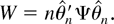
We denote by a tilde an estimator under the null hypothesis. The (quasi) LR test statistic is given by

(see equation (9)). Finally, to derive the LM test statistic

where η = (β′, σ2, θ′)′, we note that

whereas the other two partial derivatives vanish. Here,

is the jth sample autocorrelation of

.
The diagonal block of the Fisher information matrix corresponding to θ is

so the Fisher information matrix in (19) evaluated at

is n times
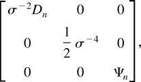
which is invertible for n sufficiently large by (4) and Assumption 2. The diagonal blocks corresponding to β and σ2 follow using that

are martingale differences, respectively. In Tanaka (1999), ζj = j−1 and Ψ = π2/6. We allow for more general weights to the autocorrelations in

, corresponding to the more flexible model represented by the function φ(z, θ). The expression

is a truncated version of Ψ, which is asymptotically equivalent to Ψ. Thus, the LM test statistic is

In the fractional unit root model (6) where ζj = j−1 we have Ψ100 = 1.5831, Ψ500 = 1.6294, and Ψ = Ψ∞ = π2/6 = 1.6449.
We derive the distribution of the test statistics under the more general assumption of local (Pitman) alternatives given by the sequence

with δ a fixed p × 1 vector.
THEOREM 3.3. Let Assumptions 1–3 be satisfied and let T denote the W, LR, or LM test statistics given by (17), (18), and (22). Then, under (23), it holds that

as n → ∞. The three tests are consistent and asymptotically equivalent; i.e., if T1 and T2 are any two of the statistics then T1 − T2 → 0 in probability. Under the additional assumption of Gaussianity they are locally most powerful.
Usually in nonstandard tests such as the Dickey–Fuller test, the three test statistics are not equivalent. From the proof we note that the equivalence of the tests depends crucially on the information matrix equality, which holds asymptotically in our model but does not hold when the unit root is nested in an autoregressive alternative.
Thus, we find that unusually simple asymptotic tests can be performed in this model using the chi-squared distribution. Also, we can easily calculate the asymptotic local power of the three test statistics, which we state as a corollary.
COROLLARY 3.1. Under the conditions of Theorem 3.3 it holds that, under

,

as n → ∞, where χp,1−α2 is the 100(1 − α)% point of the χp2 distribution and Fδ′Ψδ is the distribution function of the χp2(δ′Ψδ) distribution.
Using Corollary 3.1 we can compare the finite sample performance of the tests with the approximation offered by asymptotic theory, and we shall discuss this in Section 5.
Next, we show that even stronger results can be obtained in a subclass of models.
3.3. Uniformly Most Powerful Tests
While the general theory discussed previously applies for multidimensional θ, even stronger results are obtained in the special case of scalar θ, e.g., (6) or (7), which we now consider briefly. Following the reasoning in Elliott et al. (1996) and Tanaka (1999), we derive the power envelope for the two-sided testing problems under invariance and unbiasedness conditions and show that this two-sided power envelope is equal to (24), i.e., that this power is achieved by our tests. The unbiasedness condition is new because Elliott et al. (1996) and Tanaka (1999) only consider one-sided tests and thus do not need unbiasedness.
In particular, we assume that the errors are Gaussian and that the model in (3) is characterized by a scalar parameter θ. This rules out the general model in (5) but still applies to most of the models in Section 2. The testing problem is invariant to any transformation of the type y → ay + Xb

, or in the parameter space,

Thus, we shall restrict attention to the family of tests that are invariant to the group of transformations in (25) (see Lehmann, 1986, Chap. 6).
Assume that the DGP is given by (2) and (3), with true parameter value θ0n =

for some fixed c. Now consider testing the hypothesis H0 : θ = 0 against the sequence of local alternatives

for some fixed δ. This is a test of a simple null vs. a simple alternative with nuisance parameter (β′, σ2). Then we can apply invariance arguments to (β′, σ2) and the Neyman–Pearson lemma tells us (e.g., Lehmann, 1986, p. 338) that the test that rejects the null when
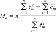
becomes large is most powerful invariant (MPI) with respect to the group of transformations (25). As in the previous section,

are residuals under H0 and H1, respectively. The next theorem derives the limiting distribution of Mn under local alternatives.
THEOREM 3.4. Let Mn denote the MPI test statistic (26), with

(c a fixed scalar) instead of θ0 = 0. Let Assumptions 1 and 2 be satisfied and suppose the error process is i.i.d. Gaussian. Then, under the sequence of local alternatives

(δ a fixed scalar), it holds that

as n → ∞, where Z is a standard normal variable.
Thus, invariance arguments have reduced the testing problem to the consideration of the statistic Mn, and the power envelope of all invariant tests is the power of M(δ, δ). Obviously, the results in Tanaka (1999) apply with little change to the corresponding one-sided testing problem in our setup and this power envelope is achieved by one-sided versions of our tests. However, because we consider mainly the two-sided testing problem, we cannot hope to achieve the same power envelope, and thus the following results differ from those in Tanaka (1999), where only one-sided hypotheses are considered.
To find a test statistic that applies against two-sided alternatives we invoke the principle of unbiasedness (see Lehmann, 1986, Ch. 4) to construct an MPI unbiased test. Unbiasedness requires that the power of the test never falls below the nominal significance level for any point in the alternative. Because for varying c the family of distributions M(c, δ) is normal, it satisfies the requirement that it be strictly totally positive of order three (STP3; see Lehmann, 1986, p. 119), and hence the power envelope of all invariant and unbiased tests of H0 : θ = 0 against

is given by Π(δ) = 1 − P(C1, α(δ) < M(δ, δ) < C2, α(δ)) (Lehmann, 1986, p. 303), where the constants are determined by


A test whose asymptotic power attains the power envelope for all points δ is asymptotically uniformly most powerful invariant unbiased. The following theorem shows that the power envelope of all invariant and unbiased tests is given by (24), i.e., that this power is achieved by our tests.
THEOREM 3.5. Let Assumptions 1 and 2 be satisfied and suppose the error process is i.i.d. Gaussian. Then the asymptotic Gaussian power envelope of all invariant (with respect to (25)) and unbiased tests of H0 : θ = 0 against

(δ a fixed scalar) is given by (24). Thus, the W, LR, and LM tests are uniformly most powerful (against local alternatives) among all invariant and unbiased tests.
This result is in stark contrast to the results of Saikkonen and Luukkonen (1993a, 1993b) and Elliott et al. (1996), among others, whose tests are only point optimal invariant, i.e., tests that have maximal power against a single prespecified (local) point in the alternative. Our criterion is against all possible (local) alternatives.
Furthermore, Theorem 3.5 also applies to the test statistic in Robinson (1994) and thus generalizes his result, too, because he only shows that his test is locally most powerful.
4. INFERENCE WITH SERIALLY CORRELATED ERRORS
Now we extend the basic model to allow for weakly dependent (ARMA) errors. In particular, we work with the following assumption.
Assumption 4. {et} is generated by an ARMA model of the form

where {εt} satisfies Assumption 3. Here a(z) and b(z) are finite polynomials without common roots and all roots strictly outside the unit circle. The coefficients in the autoregressive and moving average polynomials are collected in the q × 1 parameter vector ψ.
This assumption follows Tanaka (1999); Tanaka in addition assumes that {εt} is i.i.d. Thus, we offer more generality in this respect too, because of our martingale difference assumption on {εt}.
Collect the parameters of the dynamic part of the model in the vector γ = (θ′, ψ′)′ with true value γ0 = (0′, ψ0′)′ and let c(z, ψ) = a(z)b−1(z). Analogously to ζ(z, θ), define ξ(z, γ) = ∂ ln(φ(z, θ)c(z, ψ))/∂γ and

. Note that ξj = (ζj′, cj′)′ with ζj defined as before and cj defined as the coefficient on zj in the expansion of ∂ ln c(z, ψ)∂ψ|ψ=ψ0 in powers of z. As in Assumption 1(ii) we define

with

.
It is easily shown that Φ is the Fisher information for ψ under Assumption 4; e.g., if {et} is an AR(1) process with coefficient a then cj = −aj−1 and Φ = (1 − a2)−1. Finally, corresponding to (4), we assume that

which in particular implies that Ξ is nonsingular.
The log-likelihood function in the case of serially correlated errors is, except for constants,

to be compared with (8). The concentrated likelihood function for γ = (θ′, ψ′)′ becomes
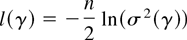
except for constants, where


and

are now defined in terms of the functions (34) and (35). Corresponding to (13) we consider the function

4.1. Estimation
The analysis of the model with serially correlated errors proceeds in the same way as with martingale difference errors as discussed previously. Thus, we are able to show the existence of a local MLE
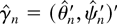
satisfying
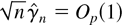
and to prove joint asymptotic normality of

. Under Gaussianity we achieve efficiency as before.
THEOREM 4.1. Under Assumptions 1, 2, and 4 and (31) there exists a local maximizer
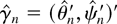
of the concentrated likelihood (33) that satisfies, as n → ∞,

Under the additional assumptions of Gaussianity of {εt} and correct (minimal) specification (all elements of ψ0 are nonzero),

is asymptotically efficient in the sense that its asymptotic variance attains the Cramér–Rao lower bound.
Based on this theorem it is possible to create joint (p + q)-dimensional confidence ellipsoids for θ and ψ that take into account the asymptotic correlation between the estimates represented by the matrix κ. This is important for inference, not only on θ but also on ψ. Usually, in applied work one would determine the appropriate filtration of data (i.e., the function φ(z, θ)) by Dickey–Fuller tests or similar methods and then treat the filtered data as if it were observed, i.e., as if the correct filter were known a priori. The resulting inference on ψ is incorrect, because the correlation between θ and ψ is ignored. When applying Theorem 4.1, this pretesting problem is avoided because θ and ψ are estimated jointly.
When inference on θ is of interest, the asymptotic marginal distribution of

can be immediately derived from the theorem.
COROLLARY 4.1. Under the conditions of Theorem 4.1,

as n → ∞.
In parallel with Corollary 4.1,

(by the partitioned matrix inverse formula), and in the special case where φ is not present this reduces to Φ−1, which is the Fisher information on ψ. Thus, the well-known asymptotic efficiency of the MLE in pure ARMA models comes out as a special case of our results. More important, Theorem 4.1 with φ present demonstrates the joint efficiency in the generalized model.
To illustrate the loss of efficiency in estimation of θ stemming from serially correlated errors, consider again the fractional unit root model. Suppose we know that the errors are not serially correlated but simply are martingale differences. Then the asymptotic variance of

is 6/π2 by Theorem 3.2. If instead it is known that the errors exhibit serial correlation of the AR(1) or MA(1) type with coefficient a, then the asymptotic variance of

is the inverse of (π2/6) − ((1 − a2)/a2)(ln(1 − a))2 by Corollary 4.1.
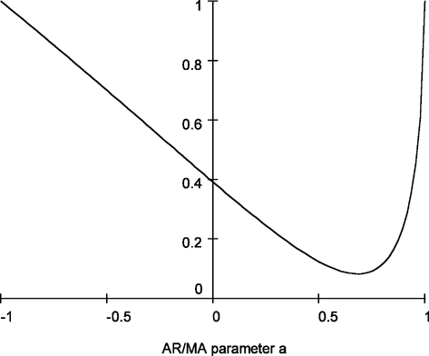
Figure 1 shows the relative efficiency of these two estimates as a function of the serial correlation parameter, a. This is calculated as
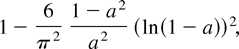
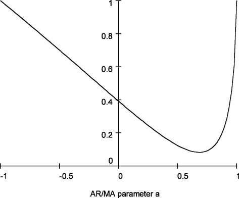
Relative efficiency of in the presence of first-order autoregressive or moving average errors.
which has a minimum at a = 0.684. This suggests that moderate levels of a best replicate the behavior of the (weighted) autocorrelations of a fractionally integrated process. The point a = 0 shows that the relative efficiency allowing for serial correlation when it is not present is 0.392, as noted by Tanaka (1999).
4.2. Hypothesis Testing
We now consider the testing problems (16) and (23) in the presence of serially correlated errors, where again only θ is of interest. The Wald, LR, and LM test statistics are

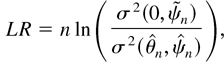

where

are evaluated at

are evaluated at

, the estimate of ψ under the null, and

is defined in terms of the jth sample autocorrelation of

.
It is obvious from the expressions for the test statistics and

that the LM test is not necessarily the simplest to apply in practice. The implementation of the Wald and LR test statistics is straightforward when we can estimate the model under both the null and alternative and should not be a problem, given the methods available in the previous sections. In particular, the LR test is attractive because there is no need to calculate Ψ, κ, and Φ.
Similar to the calculation of the infinite-order moving average coefficients in standard ARMA models, the calculation of κ and Φ can be quite cumbersome when the model in Assumption 4 is more complex than just an AR(1) or MA(1) model (see also the discussion in Tanaka, 1999). To overcome this issue, one could employ the numerical approximations

which of course have the same asymptotic properties as W and LM. However, because Ψ, κ, and Φ, and thus W and LM, can be calculated for any given parameter value (say, γ) by numerically expanding ∂ ln φ(z, θ)c(z, ψ)/∂γ at γ = γ in powers of z using a computer, we do not consider

further.
The asymptotic distribution of the tests under local alternatives and with serial correlation is given by the following theorem.
THEOREM 4.2. Let Assumptions 1, 2, and 4 and (31) be satisfied and let T denote the W, LR, or LM test statistics (39), (40), and (41). Then, under (23), it holds that

as n → ∞. The three tests are consistent and asymptotically equivalent, and under the additional assumption of Gaussianity they are locally most powerful.
This theorem shows that the tests are still locally most powerful, even in the presence of serially correlated errors. Setting κ = Φ = 0, i.e., when no serial correlation is present and ψ is not estimated, generates Theorem 3.3 as a special case. As with Corollary 3.1 in the case without serial correlation, we can easily calculate the asymptotic local power, giving us a benchmark against which to compare the power of the tests in finite samples.
COROLLARY 4.2. Under the conditions of Theorem 4.2 it holds that, under

,

as n → ∞, where χp,1−α2 is the 100(1 − α)% point of the χp2 distribution and Fδ′(Ψ−κ′Φ−1κ)δ is the distribution function of the χp2(δ′(Ψ − κ′Φ−1κ)δ) distribution.
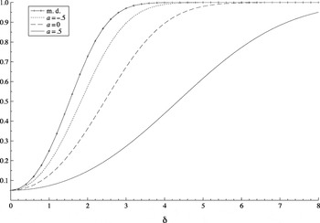
Using Corollary 4.2, Figure 2 shows the local power functions against positive alternatives for the fractional unit root model with different specifications of AR(1) errors. Because δ only enters (42) through δ2, the power functions are symmetric. The starred line is the local power function when the errors are a martingale difference sequence and this is known (i.e., using Corollary 3.1). The dotted, dashed, and solid lines correspond to AR(1) specifications of the errors with coefficient a = −0.5, a = 0, and a = 0.5, respectively. In the case a = 0, the errors are a martingale difference sequence, but an AR(1) error process is estimated.

Asymptotic local power functions with martingale difference and first-order autoregressive or moving average errors.
The local power of the tests in the model with a = 0.5 is much lower than for the other specifications. On the other hand, the power loss in the model with a = −0.5 is small. This is in accordance with the results in Section 4.1; cf. (38) and Figure 1.
5. FINITE SAMPLE PERFORMANCE
In this section, we compare the asymptotic local power functions derived in the previous sections to the finite sample rejection frequencies by means of Monte Carlo experiments.
The model we use for the simulation study is the well-known fractional unit root model with an AR(1) error:


where {εt} is i.i.d. standard normal. This model is also studied in simulations by Robinson (1994) and Tanaka (1999). In addition to this fractional DGP, Robinson (1994) also considers an autoregressive DGP and finds that his test is dominated by Dickey–Fuller type tests in the latter case.
We concentrate on comparing the finite sample performance of the three test statistics (Wald, LR, and LM). Tanaka (1999) documents that the time domain LM test outperforms Robinson's (1994) frequency domain LM test, so we do not consider the frequency domain test here. The properties of the estimator

in this model are examined by Tanaka (1999), who finds that in the case without serial correlation the behavior of the local MLE is very close to the asymptotic distribution. However, with serially correlated errors the performance of the local MLE degrades, and especially in the case of strong positive serial correlation the performance is poor. This is expected based on (38) and Figure 1.
Throughout, we fix the nominal level (type I error) at 0.05 and the number of replications at 5,000. We consider the sample sizes n = 100 and n = 500. The former is typical for macroeconomic time series and the latter (or even larger) for financial time series. For each experiment, 5,000 samples of size n = 500 were generated using the rann, diffpow, and armagen routines in Ox version 3.00 including the Arfima package version 1.01 (see Doornik, 2001; Doornik and Ooms, 2001). For the smaller sample size, n = 100, we used the first 100 out of the 500 observations from each sample.
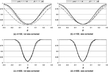
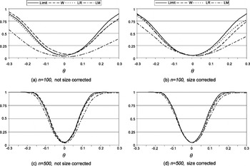
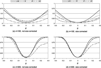
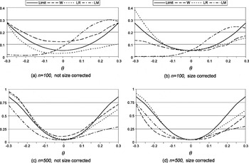
Figures 3, 4, 5, 6 present the simulated finite sample power functions of the test statistics for different specifications of the error term in (44) (the tables containing the numerical values used to construct the figures can be obtained from the author upon request). For each value of θ, the asymptotic local power has been calculated by setting

in Corollaries 3.1 and 4.2 and is reported under the heading Limit. In all the figures, the left-hand-side figures (a) and (c) present the simulated power functions of the tests calculated as in Sections 3.2 and 4.2, whereas the simulated power functions in the right-hand-side figures (b) and (d) are calculated using size corrected critical values.
First, consider the case of martingale difference errors shown in Figure 3, i.e., {et} = {εt}. In this case, all the finite sample rejection frequencies are very close to the asymptotic local power, except the LM test in the small sample n = 100, which has lower power than the LR and Wald tests.

Finite sample power functions with martingale difference errors.
When the errors are serially correlated the differences between the test statistics are more apparent. With negative serial correlation a = −0.5 (Figure 4), and with a = 0 (Figure 5), i.e., when there is no serial correlation in the DGP but an AR(1) is estimated, the LM test loses power compared to the LR and Wald tests, and the Wald test tends to be oversized in the small sample, which is also reflected by its very low size corrected power for n = 100 in Figure 5(b).

Finite sample power functions with AR(1) errors with coefficient a = −0.5.

Finite sample power functions with AR(1) errors with coefficient a = 0.
In Figure 6 the errors are positively serially correlated with a = 0.5. From the previous sections we know that the asymptotic local power is much lower in this case than with negative or no serial correlation. As Figure 6 shows, this is also the case for the finite sample rejection frequencies (note that the scaling along the vertical axis is different in Figures 6(a) and (b), compared with the other plots). In the small sample, n = 100, there are severe distortions, especially to the LM and Wald tests. The LM test completely loses power against negative alternatives, with rejection frequencies even lower than the nominal size, and the Wald test is severely oversized. When n = 500 the situation improves, but the LM test still has the lowest power and the Wald test is still severely oversized.

Finite sample power functions with AR(1) errors with coefficient a = 0.5.
Unreported simulations (which can be obtained from the author upon request) show that, not surprisingly, the performance of the LR test (with n = 100) is very bad when relevant deterministic terms are left out and that the inclusion of irrelevant mean and/or trend terms decreases power against positive values of θ. This is well known from AR-based unit root tests such as the Dickey–Fuller test, where a mean (and trend) must be included if any power against nonzero mean (and trend) is desired. However, it is worth noting that, unlike in our model, the distribution of Dickey–Fuller type test statistics changes when deterministic terms are included.
Overall, the simulations show that the improvement with respect to both size and power when considering n = 500 instead of n = 100 is substantial. Thus, one would expect very good performance of the tests in financial applications, where samples are often many times larger. In such cases, the power loss resulting from the estimation of serially correlated errors would also be of less importance. It was also found that generally the LM test has lower power than the Wald and LR tests and that the Wald test is often severely oversized. We have stressed the possibility of conducting simple asymptotic inference in our model, using the chi-squared tables, and because this property is lost if size corrected critical values must be employed, this weighs heavily against the Wald test.
Even though we concentrated on the simple and well-known fractional unit root model in the present simulation study, similar relative performance is to be expected in more complicated models such as the general model in (5). Thus, the LR test is expected to outperform the Wald and LM tests with respect to both size and power also in more complicated models.
6. CONCLUSION
We have considered likelihood inference in a wide class of potentially nonstationary univariate time series models. In such cases, inference is usually drawn in an autoregressive framework and nonstandard asymptotics apply.
In this paper we have shown that, when the estimation and testing problems are embedded in a fractional integration framework, standard asymptotics apply and desirable statistical properties of likelihood inference reemerge. In particular, there exists a local MLE that is asymptotically normal, and the classical likelihood-based tests (Wald, LR, and LM) are consistent and asymptotically chi-squared distributed under local alternatives. Under the additional assumption of Gaussianity, the local MLE is asymptotically efficient, and the tests are locally most powerful. Furthermore, in the scalar parameter case with i.i.d. Gaussian errors, our tests achieve the asymptotic Gaussian power envelope of all invariant and unbiased tests; i.e., they are asymptotically uniformly most powerful (against local alternatives) among all invariant and unbiased tests.
The Monte Carlo study shows that with sample sizes typical for macroeconomic time series the tests perform reasonably well, and with larger sample sizes such as those usually found in finance applications the performance of the tests is very good and their rejection frequencies very close to the asymptotic local power. In our Monte Carlo study the LR test dominates with respect to both size and power in finite samples. The LR test also has attractive computational features when serially correlated errors are allowed for, because it avoids a quite cumbersome calculation of covariance matrices.
The results derived in this paper could also be applied to the problem of testing for fractional cointegration when the cointegrating vector is known a priori, e.g., from economic theory. When the cointegrating vector must be estimated the results in this paper no longer apply. This presents an interesting avenue for further research which is currently under investigation by the author (see, e.g., Nielsen, 2003).
APPENDIX: PROOFS
Proof of Theorem 3.1. First, by noting that

it is immediate that the denominator in g(θ) is

by Assumption 3. The last two terms are asymptotically negligible because

by Assumption 2 and (12) and

using also uncorrelatedness of {et}.
The numerator in g(θ) can be written as


By the mean value theorem we have, for some θ* = θ*(t, n) such that 0 ≤ ∥θ*∥ ≤ ∥θ∥,
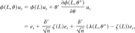
where the last term has mean zero and variance

by Assumption 1(iii) and dominated convergence. As in Robinson (1994, p. 1435), it follows that

uniformly in t. Using (A.5) we get that (A.3) is

For a fixed m > 0, consider the p-vector

and the p × p matrix

. By Assumption 3,

and applying an LLN,

in probability. The vector sequence {vt} is a martingale difference sequence with respect to the filtration

because vt is

measurable and integrable and

. for all t. Using Assumption 3,

, and by application of a martingale difference CLT (e.g., Brown, 1971; Hall and Heyde, 1980, Chap. 3.2), we establish that
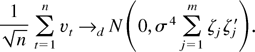
Because

can be made arbitrarily small by choosing m large by (4), we can apply Bernstein's lemma (e.g., Hall and Heyde, 1980, pp. 191–192) to conclude that (A.3) converges in distribution to δ′(2Ψ1/2Z − Ψδ)σ2. Because

we have proven the first statement of the theorem if we show that (A.2) is asymptotically negligible.
Thus, (A.2) can be written as


by (A.5), where

. Now, (A.9) is

where

uniformly in t by the same analysis as for ut, and

using (A.11) and Assumption 2. Now the second term of (A.10) is

by uncorrelatedness of {et}, Assumption 2, (4), (12), and (A.12). The same arguments apply to the first term of (A.10) and to the terms in (A.8).
Next, we examine

The expression in the first set of parentheses is
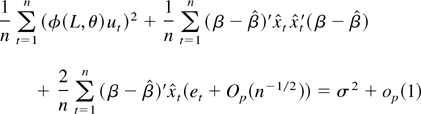
using (A.5),

as in (A.1) by Assumption 2, (12), (A.11), and (A.12).
Defining the function ζ(z, θ) = (∂/∂θ)ln φ(z, θ), the second sum in (A.13) is



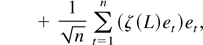
where (A.18) converges in distribution to Ψ1/2Zσ2 as in (A.6). Applying (A.5) to (A.17) we see that it equals

, which converges in probability to Ψδσ2 as in (A.6).
Thus, we need to show that (A.15) and (A.16) are asymptotically negligible. First, write (A.15) as

using (A.5). The first and third terms are Op(n−1/2) by (4) and the arguments applied to (A.14), and the second and fourth terms are Op(n−1/2) by combining the arguments applied to the first term and those applied to (A.4). Rewriting (A.16) as

using (A.5), we note that it is asymptotically negligible by the same arguments as applied to (A.4). This establishes the second statement of the theorem.
The second derivative is

which is equal to

by (A.14). Combining the preceding arguments it can be shown that the last two terms are both op(1) whereas the first term converges in probability to −Ψ. This completes the proof. █
Proof of Theorem 3.2. By Theorem 3.1(iii) and Assumption 1, g(θ) is asymptotically a concave function of

, the sphere in p-dimensional Euclidean space centered at the origin with radius

. Hence, by Theorem 3.1 and the subsequent analysis,

is asymptotically the unique maximizer of W(δ) in
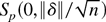
, and its asymptotic distribution is given by (15) by the usual expansion. Under Gaussianity of {et}, (8) is the true likelihood. The limiting Fisher information is then given by
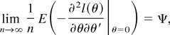
which is the inverse of the asymptotic variance as required. █
Proof of Theorem 3.3. Though the equivalence of the test statistics is well known in standard testing problems, we have stressed the nonstandard nature of our model, and thus we start by showing equivalence. By the mean value theorem

where θ* is an intermediate value. This implies that W − LM → 0 in probability by Theorem 3.1. Similarly, by a Taylor expansion of the likelihood
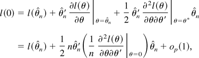
and thus LR − W → 0 in probability by Theorem 3.1(iii).
The asymptotic distribution of the test statistics follows directly from the previous theorems. Under the local alternatives (23) we set

by Theorem 3.2. Then the Wald test is

by Theorem 3.2. Similarly,

by Theorem 3.1(ii) and (21), and

by Theorems 3.1(i) and 3.2.
Under the additional assumption of Gaussianity the tests are locally most powerful because the noncentrality parameter is maximal by Theorem 3.2 and the formula for the information matrix (21). █
Proof of Corollary 3.1. This is immediate from Theorem 3.3. █
Proof of Theorem 3.4. Following the arguments of the previous sections and those in Tanaka (1999) and using (A.5) we find that
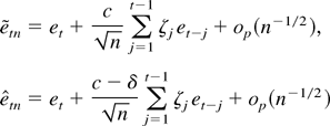
uniformly in t. Thus, the denominator of (26) normalized by n−1 converges to σ2 in probability as n → ∞, and the numerator

by the same arguments as those in the proof of Theorem 3.1. As before, it can be shown that this is unaffected by the presence of the regressors and the result follows. █
Proof of Theorem 3.5. Consider first (28), which implies that (in this context φ is the density function of the standard normal distribution)

with the nontrivial solution C1, α(δ) = −C2, α(δ) − 2δ2Ψ. Now determine the constants by (27):

where Z is a standard normal random variable. Thus, C2, α(δ) is the solution to

i.e.,

, where Z1−α/2 is the 100(1 − α/2)% point of the standard normal distribution.
The power envelope is given by

where the last line follows by squaring both sides of the inequality, χ1,1−α2 is the 100(1 − α)% point of the χ12 distribution, and Fδ2Ψ is the distribution function of the χ12(δ2Ψ) distribution. █
Proof of Theorem 4.1. The proof proceeds along the same lines as those of Theorems 3.1 and 3.2. By the same arguments it can be shown that the results are unaffected by the presence of the regressors, so we assume here that {ut} is observed.
Under

, we first show that

where Z is a (p + q)-dimensional standard normal random vector.
It is immediate that the denominator in g(γ) converges in probability to σ2 by Assumption 4. By the mean value theorem we have, for some γ* = γ*(t, n) partitioned as γ* = (θ*′, ψ*′)′ and such that ∥γ0∥ ≤ ∥γ*∥ ≤ ∥γ∥,

where λν(z, ψ) = (∂ ln c(z, ψ)/∂ψ)(c(z, ψ)/c(z, ψ0)) and λ(z, θ) is defined in Assumption 1(iii). Denoting by λν, j(ψ) the coefficient on zj in an expansion of λν(z, ψ) in powers of z and by N a neighborhood of size O(n−1/2) around ψ0,

because a(z, ψ) and b(z, ψ) have roots that are outside the unit circle. Thus, as in (A.5) it follows that

uniformly in t.
Hence, the numerator in g(γ) is

Define for a fixed m > 0 the (p + q)-vector

and the (p + q) × (p + q) matrix

. As in the proof of Theorem 3.1,

in probability, and
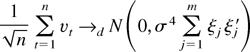
by application of a martingale difference CLT. Part (i) now follows by Bernstein's lemma.
To prove (ii) we notice that the first term in
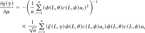
is (σ2 + op(1))−1 by (A.19) and write the second term in (A.21) as
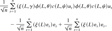
The last term converges in distribution to Ξ1/2Zσ2 as in (A.20), and by application of (A.19) the difference of the first two terms is

, which converges in probability to Ξμσ2 as in (A.20).
The result (iii) follows exactly as in the proof of Theorem 3.1.
Next, it follows as in Section 3.1 that (14) holds with δ replaced by μ and g replaced by the function in Section 4. Thus, the existence and uniqueness in

of a local MLE

satisfying
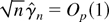
are ensured, and its distribution is given by (36) from the usual expansion.
Efficiency follows directly from (iii), which is the Fisher information under Gaussianity of {εt}. █
Proof of Corollary 4.1. Apply the partitioned matrix inverse formula to Ξ. █
Proof of Theorem 4.2. This follows straightforwardly by applying the arguments in the proof of Theorem 3.3 to the results in Theorem 4.1 and its proof. █
Proof of Corollary 4.2. This is immediate from Theorem 4.2.
References
REFERENCES
Agiakloglou, C. &
P. Newbold
(1994)
Lagrange multiplier tests for fractional difference.
Journal of Time Series Analysis
15,
253–262.CrossRefGoogle Scholar
Bierens, H.J.
(2001)
Complex unit roots and business cycles: Are they real?
Econometric Theory
17,
962–983.Google Scholar
Brown, B.M.
(1971)
Martingale central limit theorems.
Annals of Mathematical Statistics
42,
59–66.CrossRefGoogle Scholar
Chung, C.F.
(1996)
Estimating a generalized long memory process.
Journal of Econometrics
73,
237–259.CrossRefGoogle Scholar
Dickey, D.A. &
W.A. Fuller
(1979)
Distribution of the estimators for autoregressive time series with
a unit root.
Journal of the American Statistical Association
74,
427–431.Google Scholar
Doornik, J.A.
(2001)
Ox: An Object-Oriented Matrix Language,
4th ed.,
Timberlake Consultants Press.
Doornik, J.A. &
M. Ooms
(2001)
A Package for Estimating, Forecasting, and Simulating Arfima Models:
Arfima Package 1.01 for Ox.
Working Paper,
Nuffield College,
Oxford.
Elliott, G.,
T.J. Rothenberg, &
J.H. Stock
(1996)
Efficient tests for an autoregressive unit root.
Econometrica
64,
813–836.CrossRefGoogle Scholar
Engle, R.F.
(1984)
Wald, likelihood ratio, and Lagrange multiplier tests in
econometrics. In
Z. Griliches &
M.D. Intriligator (eds.),
Handbook of Econometrics,
vol. 2, pp.
775–826.
North-Holland.
Gil-Alana, L.A.
(2001)
Testing stochastic cycles in macroeconomic time series.
Journal of Time Series Analysis
22,
411–430.CrossRefGoogle Scholar
Gray, H.,
N. Zhang, &
W.A. Woodward
(1989)
On generalized fractional processes.
Journal of Time Series Analysis
10,
233–257.CrossRefGoogle Scholar
Hall, P. &
C.C. Heyde
(1980)
Martingale Limit Theory and Its Application.
Academic Press.
Hylleberg, S.,
R.F. Engle,
C.W.J. Granger, &
B.S. Yoo
(1990)
Seasonal integration and cointegration.
Journal of Econometrics
44,
215–238.CrossRefGoogle Scholar
Lehmann, E.L.
(1986)
Testing Statistical Hypotheses,
2nd ed.,
Springer-Verlag.
Ling, S. &
W.K. Li
(1997)
Fractional ARIMA-GARCH time series models.
Journal of the American Statistical Association
92,
1184–1194.CrossRefGoogle Scholar
Ling, S. &
W.K. Li
(2001)
Asymptotic inference for nonstationary fractionally integrated
autoregressive moving-average models.
Econometric Theory
17,
738–764.CrossRefGoogle Scholar
Nielsen, M.Ø.
(2003)
Optimal residual based tests for fractional cointegration and
exchange rate dynamics.
Journal of Business and Economic Statistics,
forthcoming.Google Scholar
Phillips, P.C.B.
(1987)
Time series regression with a unit root.
Econometrica
55,
277–301.CrossRefGoogle Scholar
Phillips, P.C.B. &
Z. Xiao
(1998)
A primer on unit root testing.
Journal of Economic Surveys
12,
423–469.CrossRefGoogle Scholar
Robinson, P.M.
(1991)
Testing for strong serial correlation and dynamic conditional
heteroskedasticity in multiple regressions.
Journal of Econometrics
47,
67–84.CrossRefGoogle Scholar
Robinson, P.M.
(1994)
Efficient tests of nonstationary hypotheses.
Journal of the American Statistical Association
89,
1420–1437.CrossRefGoogle Scholar
Saikkonen, P. &
R. Luukkonen
(1993a)
Point optimal tests for testing the order of differencing in ARIMA
models.
Econometric Theory
9,
343–362.Google Scholar
Saikkonen, P. &
R. Luukkonen
(1993b)
Testing for a moving average unit root in autoregressive integrated
moving average models.
Journal of the American Statistical Association
88,
596–601.Google Scholar
Sargan, J.D. &
A. Bhargava
(1983)
Maximum likelihood estimation of regression models with first order
moving average errors when the root lies on the unit circle.
Econometrica
51,
799–820.CrossRefGoogle Scholar
Sowell, F.B.
(1990)
The fractional unit root distribution.
Econometrica
58,
495–505.CrossRefGoogle Scholar
Tanaka, K.
(1999)
The nonstationary fractional unit root.
Econometric Theory
15,
549–582.CrossRefGoogle Scholar
Relative efficiency of in the presence of first-order autoregressive or moving average errors.
Asymptotic local power functions with martingale difference and first-order autoregressive or moving average errors.
Finite sample power functions with martingale difference errors.
Finite sample power functions with AR(1) errors with coefficient a = −0.5.
Finite sample power functions with AR(1) errors with coefficient a = 0.
Finite sample power functions with AR(1) errors with coefficient a = 0.5.
 You have
Access
- 25
- Cited by