1. Introduction
Conservation of magnetic helicity and efficient dynamo action make uneasy bedfellows. In an ideal fluid, magnetic helicity, which is a measure of the topological complexity and linkage of field lines (Berger & Field Reference Berger and Field1984; Moffatt & Dormy Reference Moffatt and Dormy2019), is conserved (Woltjer Reference Woltjer1958). Dynamo action is the sustained generation of magnetic energy in a fluid with finite diffusivity and often involves the generation of magnetic helicity. Clearly, when the magnetic diffusivity is small but finite (i.e. at high magnetic Reynolds number  $Rm$) the two processes become difficult to reconcile. Because dynamo action is observed to take place in nature at high
 $Rm$ some reconciliation must be achievable, but the precise form of this is the subject of intense discussion (Kulsrud & Anderson Reference Kulsrud and Anderson1992; Vainshtein & Cattaneo Reference Vainshtein and Cattaneo1992; Gruzinov & Diamond Reference Gruzinov and Diamond1994; Cattaneo & Hughes Reference Cattaneo and Hughes1996; Blackman & Field Reference Blackman and Field2002; Field & Blackman Reference Field and Blackman2002; Shukurov et al. Reference Shukurov, Sokoloff, Subramanian and Brandenburg2006; Sur, Shukurov & Subramanian Reference Sur, Shukurov and Subramanian2007).
In order to study the conservation of magnetic helicity, or lack thereof, one must define helicity precisely. This can only be achieved when the domain enclosing the ideal plasma is bounded by a flux surface (i.e. one for which the magnetic field is everywhere parallel to the surface). On the other hand, if the field ‘pokes through’ the surface, two things happen. First, the magnetic helicity is no longer gauge invariant, so some choice of gauge is required, and second boundary (flux) terms appear that allow magnetic helicity to be introduced into or removed from the domain (see e.g. Brandenburg & Subramanian Reference Brandenburg and Subramanian2005). This has led to the idea that one possible solution to the magnetic helicity problem is to assume that dynamo action predominantly occurs in systems with magnetically open boundaries where magnetic helicity can be readily expelled from (or injected into) the domain (Blackman & Field Reference Blackman and Field2000; Vishniac & Cho Reference Vishniac and Cho2001; Subramanian & Brandenburg Reference Subramanian and Brandenburg2004; Shukurov et al. Reference Shukurov, Sokoloff, Subramanian and Brandenburg2006; Ebrahimi & Bhattacharjee Reference Ebrahimi and Bhattacharjee2014; Ebrahimi & Blackman Reference Ebrahimi and Blackman2016).
Even though this idea is quite simple, its computational verification is not entirely straightforward. There are a number of issues that must be addressed. One problem is that in a magnetically open domain the magnetic helicity is not gauge invariant. Also any computational experiment at high  $Rm$ is costly. Here the problem is particularly acute because what one is mostly interested in is not merely dynamo action, but large-scale dynamo action, which involves the generation of large-scale magnetic field rather than merely the generation of magnetic energy. This problem therefore requires a separation of scales so that it is possible to separate out the large scales from the small scales. This implies that if the magnetic Reynolds number must be large on the small scales it will be enormous on the large scales. It is a fact of life that, even with the computational resources available today, one can have either large
 $Rm$ or a separation of scales – but not both in a fully nonlinear dynamo calculation. Therefore some compromise is required.
These issues were manifest in a recent work by Bodo et al. (Reference Bodo, Cattaneo, Mignone and Rossi2017), (hereinafter Part 1). They considered dynamo action driven by the magnetorotational instability within the shearing box approximation. That problem was chosen as it is known that it can lead to the generation of substantial toroidal flux and therefore large-scale dynamo action can be unambiguously identified. The requirement of large  $Rm$ was met – to some extent – by adopting a numerical code with no explicit magnetic or viscous dissipation. This kind of code is commonly used in astrophysical simulations; for given resources such codes can achieve the largest dynamic range, as they are able to resolve gradients with few grid points. The price is that, for these types of codes, there is no direct control of kinetic and magnetic Reynolds numbers. In that work the gauge problem was addressed by adopting a specific gauge – the winding gauge (Prior & Yeates Reference Prior and Yeates2014) that in their geometry provides a natural interpretation of helicity in terms of the average pairwise winding of the field lines. Bodo et al. (Reference Bodo, Cattaneo, Mignone and Rossi2017) found no clear relationship between large-scale dynamo action and the flux of magnetic helicity in and out of the domain. They speculated that this result followed from the fact that the system as a whole was nearly reflectionally symmetric and that the magnetorotational instability (MRI) dynamo is essentially nonlinear. An essentially nonlinear dynamo is one in which the dynamo velocity is itself driven or enabled by magnetic forces (see e.g. Tobias, Cattaneo & Brummell Reference Tobias, Cattaneo and Brummell2011). It is then more likely that correlations are maintained between velocity and magnetic field fluctuations, which can potentially lead to large-scale dynamo action at high
 $Rm$. An important property of these dynamos is that they have no kinematic phase. In a more conventional situation, the so-called essentially kinematic case, the dynamo velocity pre-exists independently of the magnetic field and it is only modified when the field reaches finite amplitude and causes the saturation of the dynamo. The general wisdom is that in these cases large-scale dynamo action requires a system that is not reflectionally symmetric from the outset (cf. Ebrahimi & Blackman Reference Ebrahimi and Blackman2016).
In this paper we shall address these issues in a system that is not essentially nonlinear and in which broken reflectional symmetry is externally imposed through the inclusion of a helical forcing. To that end, we consider helically forced turbulence in the presence of large-scale shear in the simplest generalisation of a periodic domain with magnetically open boundary conditions. Furthermore, and unlike in Paper 1, we want to have precise control of the diffusivities so that the Reynolds numbers can be meaningfully defined. Unfortunately this limits our analysis to moderate magnetic Reynolds numbers; so we regard the current paper as a starting point for a long-term study that will eventually inform us of the behaviour of these systems at high  $Rm$. As lack of reflectional symmetry and open boundary conditions do not necessarily guarantee large-scale dynamo action, we simply do not know in which parts of parameter space large scale dynamos can be found. At such high
 $Rm$ we would be limited to one or maybe two heroic calculations and the risk of finding something uninformative is large.
The paper is organised as follows: in the next section we give a precise formulation of the problem by describing its geometry, evolution equations, boundary conditions and forcing functions. We also define the magnetic helicity and derive its evolution equation subject to a specific choice of gauge – the winding gauge. With this choice all production and transport terms for the magnetic helicity can be unambiguously defined. In § 3 we describe and analyse the results of numerical simulations for different values of the magnetic Reynolds number and vigour of the applied shear. We provide a working definition of large-scale dynamo action in terms of either production of mean field (flux) or phase coherence (dynamo waves). We identify dynamo solutions and distinguish those in which a large-scale magnetic field is generated. For these solutions, and in keeping with our objectives, we compare the evolution of the magnetic helicity and the properties of large-scale dynamo action. Concluding remarks and possible directions for future work are included in § 4. Finally, we note that, hereinafter, the term helicity by itself will be taken to mean the magnetic helicity as defined in § 2. References to other types of helicities will be made explicitly.
2. Formulation of the problem
As noted in the introduction, well-resolved dynamo calculations are difficult. We therefore consider a highly idealised system that has all of the essential features; lack of reflectional symmetry, magnetically open boundaries and the presence of shear, but is also designed to be computationally efficient. To this end we consider a cartesian domain in which two of the directions (the ‘horizontal’ directions) are periodic and in the third (‘vertical’) direction the boundaries are picked so that they are magnetically open. With this choice, fluxes (i.e. surface integral terms) have to be computed on only the two horizontal surfaces. The flow is driven by two body forces; one chosen so that it drives a horizontal shear flow. The second force drives a small-scale strongly helical flow with good dynamo properties. A good candidate for driving this small-scale flow is a generalisation of the Galloway–Proctor forcing (i.e. the forcing that at low Reynolds number,  $Re$, drives the Galloway–Proctor flow (Galloway & Proctor Reference Galloway and Proctor1992)) – however, this requires periodic boundary conditions in all three directions. It is relatively straightforward to modify this forcing so that it drives a helical flow that is compatible with impenetrable, stress-free boundary conditions, see appendix A for further details.
We consider dynamo action in a Cartesian domain  $(x,y,z)$ of size
 $(2{\rm \pi} , 2{\rm \pi} , {\rm \pi} )$. We solve the non-dimensional induction equation
 \begin{equation} \dfrac{\partial \boldsymbol{B}}{\partial t} = \boldsymbol{\nabla}\times(\boldsymbol{u} \times \boldsymbol{B})-\eta \boldsymbol{\nabla} \times \boldsymbol{J}, \end{equation}
together with the incompressible non-dimensional Navier–Stokes equation
 \begin{equation} \dfrac{\partial \boldsymbol{u}}{\partial t} + \boldsymbol{u} \boldsymbol{\cdot} \boldsymbol{\nabla} \boldsymbol{u} = - \boldsymbol{\nabla} \boldsymbol{p}+ \boldsymbol{J} \times \boldsymbol{B} + \nu \nabla^2 \boldsymbol{u} + \boldsymbol{f}, \end{equation}
and the solenoidal conditions
 \begin{equation} \boldsymbol{\nabla} \boldsymbol{\cdot} \boldsymbol{u} = \boldsymbol{\nabla} \boldsymbol{\cdot} \boldsymbol{B} = 0, \end{equation}
for the velocity  ${\boldsymbol {u}}=(u,v,w)$ and magnetic field
 $\boldsymbol {B}=(B_x,B_y,B_z)$. Here,
 $\eta$ is the non-dimensional magnetic diffusivity,
 $\nu$ the non-dimensional viscosity, the current density
 $\boldsymbol {J}=\boldsymbol {\nabla } \times \boldsymbol {B}$ and
 $\boldsymbol {f}$ is a body force. The non-dimensionalisation is effected by choosing the vertical size of the domain as
 ${\rm \pi}$ times the unit of length, the root-mean-square (r.m.s.) velocity as the unit of velocity and by measuring the magnetic field intensity in units of the equivalent Alfvén speed. We solve equations (2.1)–(2.3) subject to periodic boundary conditions in the two horizontal directions and impermeable, stress-free boundary conditions on the velocity in the vertical
 $z$ direction. The magnetic boundary conditions for the field
 $\boldsymbol {B}=(B_x,B_y,B_z)$ are ‘vertical’ boundary conditions where the magnetic field is constrained to be vertical on the upper and lower boundaries. Mathematically these translate to
 \begin{equation} \dfrac{\partial u}{ \partial z} = \dfrac{ \partial v}{\partial z} = w = 0, \end{equation}
together with
 \begin{equation} B_x= B_y = 0. \end{equation}
Notice that these boundary conditions are compatible with a sine/cosine expansion of all the variables in  $z$, which allows the solution by Fourier pseudo-spectral methods.
The forcing  $\boldsymbol {f}$ is given by
 \begin{equation} {\boldsymbol{f}} =\boldsymbol{G}({x,z,t})+S (\cos z,0,0). \end{equation}
Here, the small-scale forcing  $\boldsymbol {G}$ is a helical vector function that satisfies the same boundary conditions as the velocity. Its spatial structure is given by the superposition of strongly helical cellular vector fields and is best described in terms of its Fourier representation – see appendix A. We note here that we choose a typical scale separation between the cellular forcing and the domain of approximately 6 to 8; i.e. the small-scale forcing is a superposition of cellular fields with horizontal wavenumber,
 $k$, between 6 and 8.
2.1. Gauges, helicity and fluxes
The objective of this paper is to monitor the evolution of the magnetic helicity and to relate it to episodes of dynamo activity. For this we require a reasonable definition of the magnetic helicity. We begin by introducing the vector potential  $\boldsymbol {A}$ by setting
 \begin{equation} \boldsymbol{B}= \boldsymbol{\nabla} \times \boldsymbol{A}. \end{equation}
Clearly,  $\boldsymbol {A}$ is not unique and the gauge transformation
 \begin{equation} \boldsymbol{A} \rightarrow \boldsymbol{A} + \boldsymbol{\nabla} \psi \end{equation}
leaves the magnetic field  $\boldsymbol {B}$ unchanged. Uniqueness can be restored by introducing an extra gauge condition on
 $\boldsymbol {A}$ so that
 $\psi$ can be defined uniquely. In this paper we chose the winding gauge that requires the vector potential to satisfy
 \begin{equation} \nabla_H \boldsymbol{\cdot} \boldsymbol{A} = 0, \quad \textrm{where} \ \nabla_H \equiv (\partial_x, \partial_y, 0). \end{equation}
Hereinafter, a subscript ‘ $H$’ will denote a vector quantity whose third component (
 $z$-direction) vanishes identically. As shown by Prior & Yeates (Reference Prior and Yeates2014), for a cylindrical domain with sides that are flux surfaces and with magnetically open top and bottom surfaces, the helicity in the winding gauge gives the average pairwise winding of field lines.
We now proceed by defining all relevant quantities in this gauge. The evolution equation for the vector potential can be obtained by ‘uncurling’ the induction equation (2.1) to give
 \begin{equation} \partial_t \boldsymbol{A} - \boldsymbol{\nabla} \Phi=(\boldsymbol{u}\times \boldsymbol{B})-\eta \boldsymbol{J}, \end{equation}
where  $\Phi$ is related to the choice of gauge
 $(\Phi = - \partial _t \psi )$.
To compute  $\boldsymbol {A}$, we note that
 \begin{equation} \boldsymbol{J} = \boldsymbol{\nabla} \times \boldsymbol{\nabla} \times \boldsymbol{A} = -\nabla^2 \boldsymbol{A} + \boldsymbol{\nabla} (\boldsymbol{\nabla} \boldsymbol{\cdot} \boldsymbol{A})=-\nabla^2 \boldsymbol{A} + \boldsymbol{\nabla} \left(\frac{\partial}{\partial z} A_z \right), \end{equation}
because of our choice of gauge condition. In component form (2.11) becomes
 \begin{equation} \boldsymbol{J}_H - \nabla_H \left(\frac{\partial}{\partial z} A_z \right)= - \nabla^2 \boldsymbol{A}_H \quad \textrm{and} \quad J_z= - \nabla_H^2 A_z. \end{equation}
Clearly the  $z$-component can be solved first to give
 $A_z$, which in turn can be used to solve for the two horizontal components. Because of our boundary conditions: periodic in the horizontal and ‘vertical’ in
 $z$,
 $\boldsymbol {A}$ as defined by (2.11), is still arbitrary up to a transformation of the form
 \begin{equation} \boldsymbol{A} \rightarrow \boldsymbol{A} + \boldsymbol{A}_0, \quad \textrm{with} \ \boldsymbol{A}_0= \left(a_x(t),a_y(t),0\right). \end{equation}
We shall return to this point presently. The scalar function  $\Phi$ can likewise be computed by taking the horizontal divergence of (2.10) and using the winding gauge condition to give
 \begin{equation} \nabla_H^2 \Phi' = - \nabla_H \boldsymbol{\cdot} (\boldsymbol{u} \times \boldsymbol{B}) \quad \textrm{with } \ \Phi= \Phi' + \eta \frac{\partial}{\partial z} A_z. \end{equation}
Again, because of the periodic boundary conditions,  $\Phi$ is arbitrary up to transformations of the form
 \begin{equation} \Phi \rightarrow \Phi + \Psi, \quad \textrm{where} \ \Psi = \boldsymbol{C}_H(t) \boldsymbol{\cdot} \boldsymbol{x}. \end{equation}
Clearly, the functions  $\boldsymbol {A}_0(t)$ and
 $\Psi (t)$ arise because, with our choice of boundary conditions, the horizontal Laplacian has a non-trivial null space. Consequently, in our geometry, the winding gauge condition alone is not sufficient to specify the vector potential uniquely. To remove the remaining arbitrariness we note that in (2.10),
 $\boldsymbol {A}_0$ and
 ${\Psi }$ only occur in the combination
 $\dot {\boldsymbol {A}}_0 -\boldsymbol {\nabla } \Psi$, so that the time dependence can be assigned to either quantity. Taking this into account we choose
 $\boldsymbol {A}_0 \equiv {\bf 0}$. This choice has the desirable property that it assigns zero helicity to a purely unidirectional horizontal field in a static medium. Then, since
 $\langle \boldsymbol {J} \rangle = \langle \boldsymbol {A} \rangle =0$,
 $\Psi$ is uniquely determined by the volume average of (2.10) which gives
 \begin{equation} \Psi = -\langle \boldsymbol{u} \times \boldsymbol{B} \rangle_H \boldsymbol{\cdot} \boldsymbol{x}, \quad \textrm{with} \ \langle \Phi \rangle = \boldsymbol{\nabla} \langle \Phi \rangle =0, \end{equation}
where the angle brackets denote a volume average.
We now define the magnetic helicity  $H$ by
 \begin{equation} H=\int_V \boldsymbol{A} \boldsymbol{\cdot} \boldsymbol{B}\,\textrm{d}V, \end{equation}
where the integral is over the entire domain. By use of the evolution equations for  $\boldsymbol {A}$ and
 $\boldsymbol {B}$ above, we can readily obtain an evolution equation for the helicity in the winding gauge, this reads
 \begin{equation} \frac{\textrm{d}H}{\textrm{d}t} = W_H + F_I + W_D+F_D+F_G, \end{equation}
where
 \begin{equation} W_H= - \textrm{V} _0 \langle \boldsymbol{u} \times \boldsymbol{B} \rangle \boldsymbol{\cdot} \langle \boldsymbol{B} \rangle_H, \end{equation}
 \begin{equation}F_I= \int_S (\boldsymbol{B} \boldsymbol{\cdot} \boldsymbol{n}) [ \boldsymbol{A} \boldsymbol{\cdot} \boldsymbol{u} + \Phi' ]\,\textrm{d}S, \end{equation}
 \begin{equation}W_D= - 2\eta \textrm{V} \langle \boldsymbol{B} \boldsymbol{\cdot} \boldsymbol{J} \rangle, \end{equation}
 \begin{equation}F_D= \eta \int_S (\boldsymbol{A}\times \boldsymbol{J}) \boldsymbol{\cdot} \boldsymbol{n} \,\textrm{d}S, \end{equation}
and
 \begin{equation} F_G= \eta \int_S ( \boldsymbol{B} \boldsymbol{\cdot} \boldsymbol{n}) \frac{\partial}{\partial z } A_z \,\textrm{d}S. \end{equation}
Here,  $V_0$ is the volume of the whole domain,
 $S$ is the union of the upper and lower boundaries and n is the outward unit normal. Clearly, if
 $\eta =0$ and the domain is simply connected and bounded by a comoving flux surface then all the terms on the right-hand side of (2.18) vanish identically and the helicity is both constant and gauge invariant. In this paper, however,
 $\eta >0$, the domain is not simply connected, nor is it bounded by a flux surface, so the helicity both depends on the choice of gauge and changes with time.
The first term on the right-hand side evolves the linkage between the mean horizontal field and mean electromotive force (e.m.f.)  $\langle \boldsymbol {u} \times \boldsymbol {B} \rangle$; its presence is a consequence of our periodic boundary conditions (plus shear) and, for instance, would be absent in the geometry considered by Prior & Yeates (Reference Prior and Yeates2014). The second term (2.20) depends explicitly on the gauge function and represents an ideal flux of helicity through the open top and bottom boundaries; it would vanish if these were flux surfaces. The third term (2.21) measures the rate of helicity generation due to diffusive processes in the interior (reconnection). The fourth is a diffusive flux of helicity through the open boundaries; it would be non-zero even if these boundaries were flux surfaces. Finally, the last term (2.23) is the diffusive flux of helicity through the vertical boundary necessary to enforce our gauge condition.
One of the convenient features of expression (2.18) is that in numerical simulations both its left-hand side and right-hand side can be calculated independently. Their equality increases one's confidence that all the terms that contribute to the rate of change of the helicity are accounted for, and that the simulation itself cannot be completely off. Mercifully, that is indeed the case in our studies.
3. Results
We examine the evolution of the dynamo system using the following procedure. We first integrate the hydrodynamic equations until a statistically steady state is reached. As we are using a low Reynolds number, this state is reached rapidly (within an order one time scale). These states have the following hydrodynamic properties. At low Reynolds numbers (large values of  $\nu$) the resulting non-magnetic flow is quasi-cellular in
 $x$ and
 $z$, is independent of
 $y$ and has a characteristic scale in
 $x$ and
 $z$ of
 $2 {\rm \pi} /k$. Such
 $2{\frac{1}{2}}$-dimensional flows have been utilised in a number of dynamo studies (see e.g. Roberts Reference Roberts1972; Galloway & Proctor Reference Galloway and Proctor1992; Tobias & Cattaneo Reference Tobias and Cattaneo2008). The strength of the forcing is such that for a given
 $Re$ the resulting unmagnetised unsheared flow has approximately unit amplitude. That being the case the Reynolds numbers on the scale of the cellular flow are of the order of
 $Rm \sim 1/\eta k$ and
 $Re \sim 1/ \nu k$ respectively. The forcing may also drive a unidirectional shear
 $(U(z),0,0)$ at low values of
 $Re$, with an amplitude controlled by
 $S$. This flow combination has been used successfully in periodic domains to examine the kinematic growth of large-scale magnetic field at extremely high magnetic Reynolds number (of
 ${\textit{O}}(10^5)$) (Tobias & Cattaneo Reference Tobias and Cattaneo2013, Reference Tobias and Cattaneo2015; Nigro et al. Reference Nigro, Pongkitiwanichakul, Cattaneo and Tobias2017) and the nonlinear saturation of such dynamos (albeit at more moderate magnetic Reynolds numbers of
 ${{\textit{O}}}(10^2)$) in a triply periodic domain (Pongkitiwanichakul et al. Reference Pongkitiwanichakul, Nigro, Cattaneo and Tobias2016). To the saturated stationary hydrodynamic state we add a small random seed magnetic field, which is then amplified by kinematic dynamo action and saturates in a statistically steady state that depends on the value of the shear and
 $\eta$ selected.
We consider in detail 9 cases in which we vary the shear by setting  $S=0, 1, 5$ and the magnetic diffusivity
 $\eta = \eta ^0 \cdot (1,1/2,1/4)$, with
 $\eta _0 = 0.0125$ – this corresponds to magnetic Reynolds numbers
 $R_m = 10, 20, 40$. In all cases we fix the resolution at
 $(nx,ny,nz) = (256,256,257)$, which is large enough to resolve the dissipative structures in the magnetic field. The viscosity is kept constant so that the magnetic Prandtl number takes the corresponding values of
 $\nu / \eta = 200 \cdot (1,2,4)$. The reason for this choice is to ensure that for all the cases the magnetic Reynolds number is large enough to trigger dynamo action while at the same time the Reynolds number
 $Re$ remains small. For higher values of
 $Re$ the basic hydrodynamic flow becomes unstable, and eventually turbulent and it is difficult to control the kinetic helicity or the amplitude of the shear – this regime forms the basis for a subsequent paper. In the low
 $Re$ regime studied here, with high
 $Pm$, when the dynamo operates eventually the magnetic energy typically greatly exceeds the kinetic energy (Brummell, Cattaneo & Tobias Reference Brummell, Cattaneo and Tobias2001).
All cases considered display a well-defined kinematic phase, which is typically short lived, in which the magnetic energy increase exponentially. This phase is quickly followed by a nonlinear readjustment of the flow and field and the establishment of one of possibly many statistically stationary states. In general, the nonlinear states are very different from the kinematic ones. In some cases, in the nonlinear regime, the dynamo swaps between different states. Depending on the values of the magnetic diffusivity  $\eta$ and shear parameter
 $S$ we observe a variety of different nonlinear dynamo behaviours. Broadly speaking, we can distinguish between two different classes, those in which there is evidence for propagating large-scale structures, such as dynamo waves, and those in which no propagation is apparent. In general propagating behaviour is observed, for the same value of
 $\eta$, at higher values of the shear parameter
 $S$.
3.1. Dynamo solutions
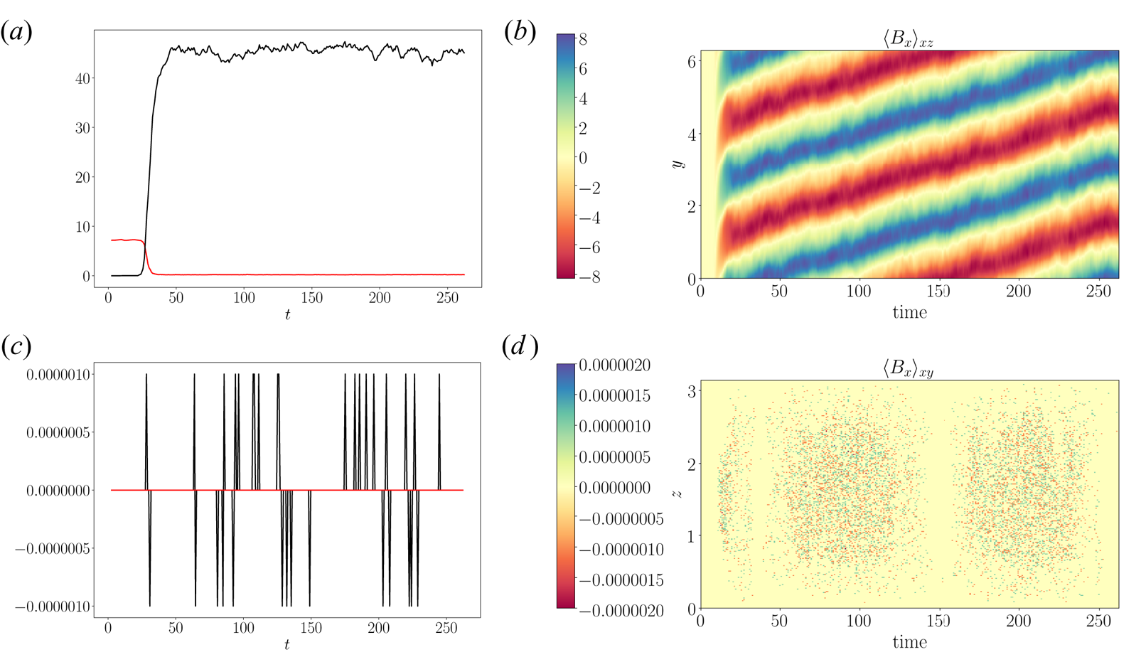
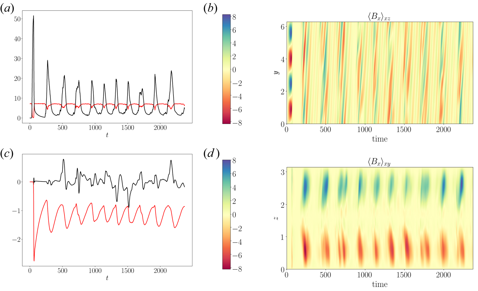
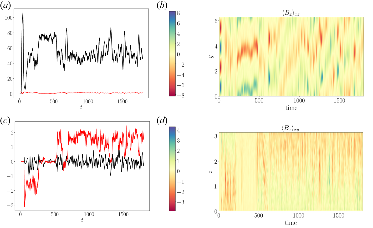
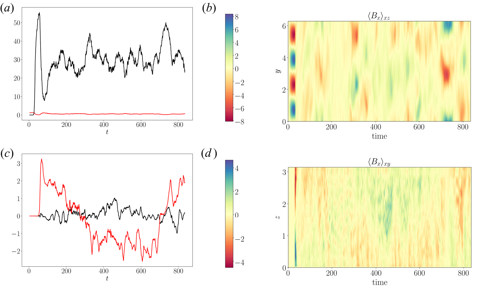
We illustrate some of the dynamo features of four representative solutions in figures 1–4, before examining in detail the role of magnetic helicity in § 3.2. These show the time histories of the kinetic and magnetic energies, and, in order to reveal possible large-scale organisation, the time histories of the volume averaged values of  $B_x$ and
 $B_y$. In addition, we give Hovmoller plots of
 $B_x$ volume averaged in
 $x$ and
 $z$, and
 $x$ and
 $y$, which are designed to show the form of the large-scale (averaged structures) in the toroidal field.
(a) Time histories of magnetic (black curve) and kinetic (red curve) energies; (c) time histories of the volume averaged values of  $B_x$ (black curve) and
 $B_y$ (red curve); (b) Hovmoller plot of
 $\langle B_x \rangle _{xz}(t,y)$; (d) Hovmoller plot of
 $\langle B_x \rangle _{xy}(t,z)$. The case is with
 $S=5$ and low
 $Rm=10$.

(a) Time histories of magnetic (black curve) and kinetic (red curve) energies; (c) time histories of the volume averaged values of  $B_x$ (black curve) and
 $B_y$ (red curve). The energy in the mean magnetic field is approximately
 $5 \%$ of the total magnetic energy; (b) Hovmoller plot of
 $\langle B_x \rangle _{xz}(t,y)$; (d) Hovmoller plot of
 $\langle B_x \rangle _{xy}(t,z)$. The case is with
 $S=5$ and moderate
 $Rm=20$.

(a) Time histories of magnetic (black curve) and kinetic (red curve) energies; (c) time histories of the volume averaged values of  $B_x$ (black curve) and
 $B_y$ (red curve). The energy in the mean magnetic field is approximately
 $3 \%$ of the total magnetic energy; (b) Hovmoller plot of
 $\langle B_x \rangle _{xz}(t,y)$; (d) Hovmoller plot of
 $\langle B_x \rangle _{xy}(t,z)$. The case is with
 $S=1$ and moderate
 $Rm=20$.

(a) Time histories of magnetic (black curve) and kinetic (red curve) energies; (c) time histories of the volume averaged values of  $B_x$ (black curve) and
 $B_y$ (red curve). The energy in the mean magnetic field is approximately
 $2 \%$ of the total magnetic energy; (b) Hovmoller plot of
 $\langle B_x \rangle _{xz}(t,y)$; (d) Hovmoller plot of
 $\langle B_x \rangle _{xy}(t,z)$. The case is with
 $S=1$ and high
 $Rm=40$.

The first case (figure 1) has  $S=5$ and high
 $\eta$ (low
 $Rm = 10$). The magnetic energy settles down into a statistically steady state with small variations about a well-defined mean value. The large-scale structure of the kinematic solution consists of a pair of
 $y$-propagating dynamo waves
 $(k_y=2)$, as shown in figure 1(b). By
 $t=25$ the kinematic state is seamlessly replaced by the nonlinear solution which also consists of a pair of nonlinear
 $y$ propagating waves, albeit with much lower phase speed; this can be seen by the change in slope of the bands in the Hovmoller plot. In this solution no mean field is generated (
 $\langle \boldsymbol {B} \rangle =0$ as shown in figure 1c). We shall return to the issue of the large change in frequency and the lack of mean field presently. Here,we note that this is the only case we have found in which the dominant
 $y$-wavenumber remains unchanged as the solution becomes nonlinear.
The second case (figure 2) has strong shear ( $S=5$) and moderate
 $\eta$ (
 $R_m = 20$). Again, the kinematic solution consists of a pair of
 $y$-propagating dynamo waves, however, this solution is quickly disrupted and replaced by a nonlinear state consisting of a travelling, pulsating wave with
 $k_y=1$, i.e. with a larger scale than the kinematic solution. Unlike in the previous case, here, the phase speed actually increases slightly as the solution becomes nonlinear, presumably owing to the change in wavenumber. The pulsations are most apparent in the magnetic energy time traces (figure 2a) as well as in the
 $x-y$ averaged Hovmoller plots in figure 2(d). The period of the pulsations is not directly related to the phase speed of the wave. The pulsations also correspond to a vigorous production of mean (over the whole domain)
 $B_y$ with no systematic corresponding production of
 $B_x$, we shall return to this in § 3.2.
The third case has weak shear ( $S=1$) and moderate
 $\eta$ –
 $R_m = 20$ – (figure 3). The kinematic solution consists of a non-propagating (or very slowly propagating) structure with
 $k_y=2$. Again, this is quickly disrupted and the system transitions to a series of nonlinear states with
 $k_y=1$. Both non-propagating
 $(t< 800)$ and propagating solutions
 $(t> 800)$ are apparent in the Hovmoller plot of figure 3(b). Interestingly, the propagation direction reverses around
 $t=1100$. Again, we note the pronounced production of mean
 $B_y$ with no corresponding production of mean
 $B_x$ (as shown in figure 3c).
Finally, the fourth case has (weak shear)  $S=1$ and low
 $\eta$ (high
 $Rm = 40$) and is shown in figure 4. Here the overall solution is similar to that of the previous case but with no episodes of propagation. As before, mean
 $B_y$ is readily produced with the occasional sign change, as shown in figure 4(c). We also note the following points from the cases not shown here: the solutions with no shear (i.e.
 $S=0$) resemble this last case, while decreasing
 $\eta$ (increasing
 $Rm$) for high shear
 $S=5$, results in a propagating, pulsating wave, much as in the case with moderate
 $\eta$. This wave at higher
 $Rm$ has a slightly lower phase speed and longer pulsation period.
3.2. Large-scale dynamo action: magnetic energy and helicity
Our main motivation is to examine the relationship between large-scale dynamo action and the creation and transport of magnetic helicity. This requires the clarification of what is meant by large-scale dynamo action so that such episodes can be identified. We note that, with our geometry and boundary conditions,  $\langle B_z \rangle$ is conserved but
 $\langle B_y \rangle$ and
 $\langle B_x \rangle$ are not. Thus, for instance we could identify ‘large-scale’ dynamo action exclusively with the net generation of magnetic flux in the
 $x$ or
 $y$ direction. This, however, may be too restrictive. There could be large-scale structures that should still be identified as evidence of large-scale dynamo action that do not give rise to substantial amounts of net flux, because, for instance, they are anti-symmetric with respect to the midplane. (We recall that large-scale dynamo action is universally acknowledged to be taking place in the Sun, though the net toroidal flux is antisymmetric about the equator.) Thus, here, we identify a large-scale dynamo with either the substantial generation of horizontal flux, or the presence of well defined propagating structures (i.e. those with spatio-temporal phase coherence; see Nigro et al. (Reference Nigro, Pongkitiwanichakul, Cattaneo and Tobias2017)). For the purpose of this discussion, a substantial amount of flux is one that substantially exceeds that which is compatible with a strong suppression of the
 $\alpha$-effect (Vainshtein & Cattaneo Reference Vainshtein and Cattaneo1992). With this definition in mind, we examine three representative cases, namely
 $S=1$, low
 $\eta$ (high
 $R_m = 40$),
 $S=5$ high
 $\eta$ (low
 $R_m = 10$ and
 $S=5$ moderate
 $\eta$ (
 $R_m = 20$).
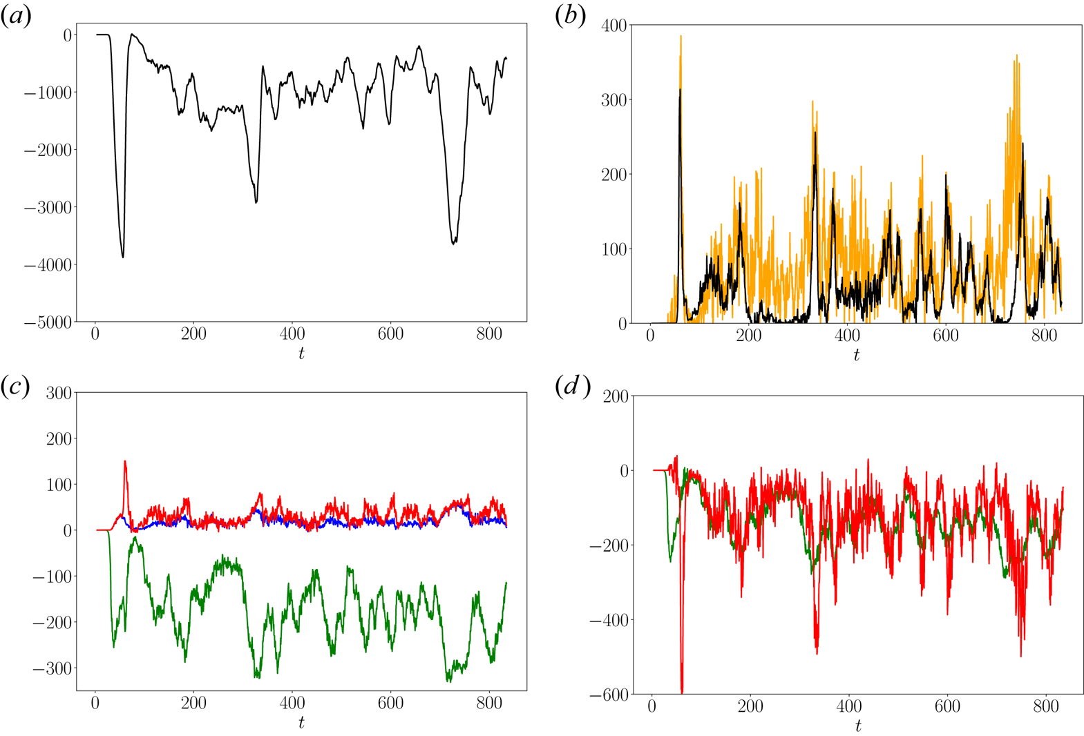
Figure 5 shows the time history of the total helicity as well as the time histories of all of the terms on the right-hand side of (2.18) for the first case with  $S=1$, low
 $\eta$ (high
 $Rm=40$). The total helicity for this case is negative and fluctuating, with three prominent peaks that roughly correspond to the three peaks in the magnetic energy. We note the following general features; the term that mostly drives the growth of helicity is the volumetric diffusive term
 $W_D$. The other two diffusive terms, both surface fluxes, only contribute after the volumetric terms has caused a substantial growth of (negative) helicity. The same is true for the ideal terms, both the volumetric and surface flux. A stationary state is reached because the helicity production by the
 $W_D$ term is approximately balanced by the sum of all the other terms. It is noteworthy that the three peaks in the helicity correspond to the epochs when both components of the mean horizontal field are small and therefore there is no contribution to the helicity destruction by the volumetric terms
 $W_H$.
(a) Time history of the helicity; (b) time histories of the ideal terms  $F_I$ (orange curve) and
 $W_H$ (black curve); (c) time histories of the diffusive terms
 $W_D$ (green curve),
 $F_D$ (red curve) and
 $F_G$ (blue curve); (d) time histories of the sum of all ideal terms (red curve) and of all diffusive terms (green curve). The case is with
 $S=1$ and high
 $Rm=40$.

The next case with  $S=5$ and high
 $\eta$ (
 $R_m =10$) yields
 $y$-propagating dynamo waves. As we mentioned above, the phase velocity decreases sharply in the transition between the kinematic and the nonlinear phases and no mean field is generated. Both of these features are related to spectral symmetries of the solution as follows. Let us begin by noting that there is a subset of the possible solutions in which the velocity's Fourier components have
 $y$-wavenumbers of the form
 $k_y=4(\,j-1)$,
 $j \in \mathbb {Z}^+$ and the magnetic field's components have wavenumbers of the form
 $k_y=4(\,j-1/2)$,
 $j \in \mathbb {Z}^+$. Clearly, the kinematic solutions in which the velocity is entirely
 $y$-independent and the magnetic field consists of a single ‘eigenmode’ with
 $k_y=2$ are all contained in this subset. These symmetries are preserved because of the nature of the nonlinearities of the induction and momentum equations. For large values of
 $\eta$ this invariant subset is stable, so that initial conditions in the subset remain in the subset. Thus there is no mean field generated; that would require the interaction between Fourier components of the velocity and magnetic field with the same wavenumbers. Moreover, in this case, the projection of the Lorentz force onto the
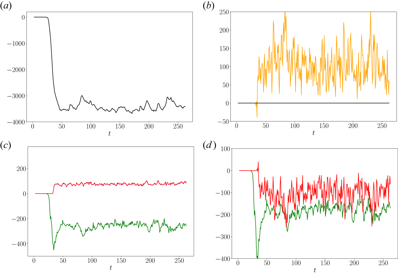
 $k_y=0$ subspace is such that it can efficiently reduce the shear. This leads to a corresponding reduction of the phase velocity of the dynamo waves, since the frequency of the dynamo waves is controlled inter alia by the strength of the shear. From figure 6 we see that, as for the previous case, the total helicity is negative, and its growth is driven by
 $W_D$, and eventually limited by the growth of the flux terms. We note that in cases like this one, in which the mean horizontal fields vanish identically,
 $W_H=0$. Moreover, the diffusive flux terms
 $F_D$ and
 $F_G$ are identical. Even though it may not be obvious from their definitions it is nevertheless true. In figure 6(c) both curves are plotted but only one is visible because they perfectly lie on top of each other.
(a) Time history of the helicity; (b) time histories of the ideal terms  $F_I$ (orange curve) and
 $W_H$ (black curve); (c) time histories of the diffusive terms
 $W_D$ (green curve),
 $F_D$ (red curve) and
 $F_G$ (blue curve); (d) time histories of the sum of all ideal terms (red curve) and of all diffusive terms (green curve). The case is with
 $S=5$ and low
 $Rm=10$.

Finally, we consider the case with  $S=5$ and moderate
 $\eta$ –
 $R_m = 20$ – (see figure 7). This case consists of pulsating travelling dynamo waves. Unlike in the previous case, here, the invariant manifold is now unstable and the kinematic solution is completely destroyed in the transition to the nonlinear phase. It is replaced by a pulsating travelling wave with
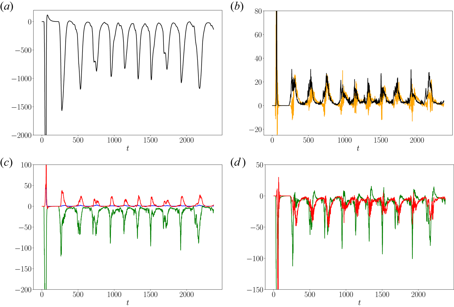
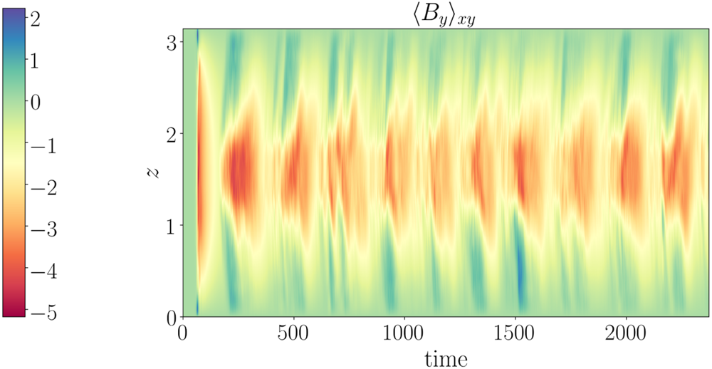
 $k_y=1$. Once the solution spreads outside the invariant manifold, it loses the ability to reduce the shear effectively and the resulting nonlinear phase speed remains close to the kinematic one. Pulsations are then superposed on these high speed travelling waves. Away from a pulsation, the magnetic energy is small and lower than the kinetic energy, and the total magnetic helicity is close to zero. During a pulsation the magnetic energy first rises quickly to a value several times the kinetic energy and then decreases again. There is a corresponding cycle in the growth of (negative) total magnetic helicity. During the pulsation the shear is slightly reduced with a corresponding reduction in the overall kinetic energy. Along with the increase in magnetic energy there is also a corresponding increase in the amplitude of a symmetric (with respect to the midplane)
 $\langle B_y \rangle _{xy}$, as shown in figure 8, and anti-symmetric
 $\langle B_x \rangle _{xy}$ as illustrated in figure 2(d).
(a) Time history of the helicity; (b) time histories of the ideal terms  $F_I$ (orange curve) and
 $W_H$ (black curve); (c) time histories of the diffusive terms
 $W_D$ (green curve),
 $F_D$ (red curve) and
 $F_G$ (blue curve); (d) time histories of the sum of all ideal terms (red curve) and of all diffusive terms (green curve). The case is with
 $S=5$ and moderate
 $Rm=20$.

Hovmoller plot of  $\langle B_y \rangle _{xy}(t,z)$ for case
 $S=5$ moderate
 $Rm=20$.

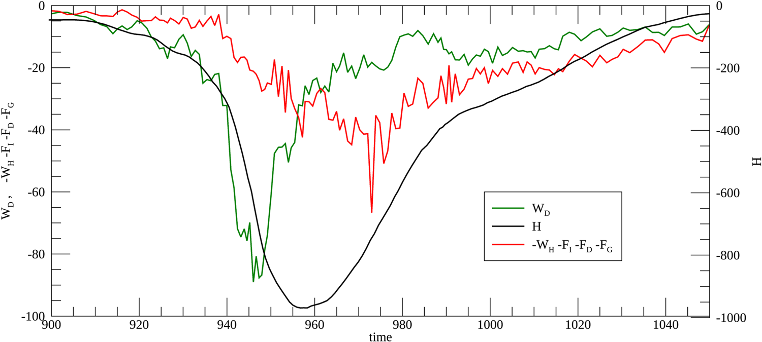
In order better to understand the terms that lead to the growth and eventual decay of the helicity it is useful to look in more details at a single pulsation. To this end we plot in figure 9 the time histories of the helicity,  $W_D$, and the sum of the rest of the terms in (2.18) over the pulse centred around
 $t=960$. As before, the increase in (negative) helicity is driven by the sharp rise in
 $W_D$. The subsequent decrease in helicity is caused by the rise in all the other terms, both volumetric and fluxes, and by the abrupt switching off of the production term shortly before the helicity reaches its peak
 $(t \sim 950)$. We note that the abrupt decrease in
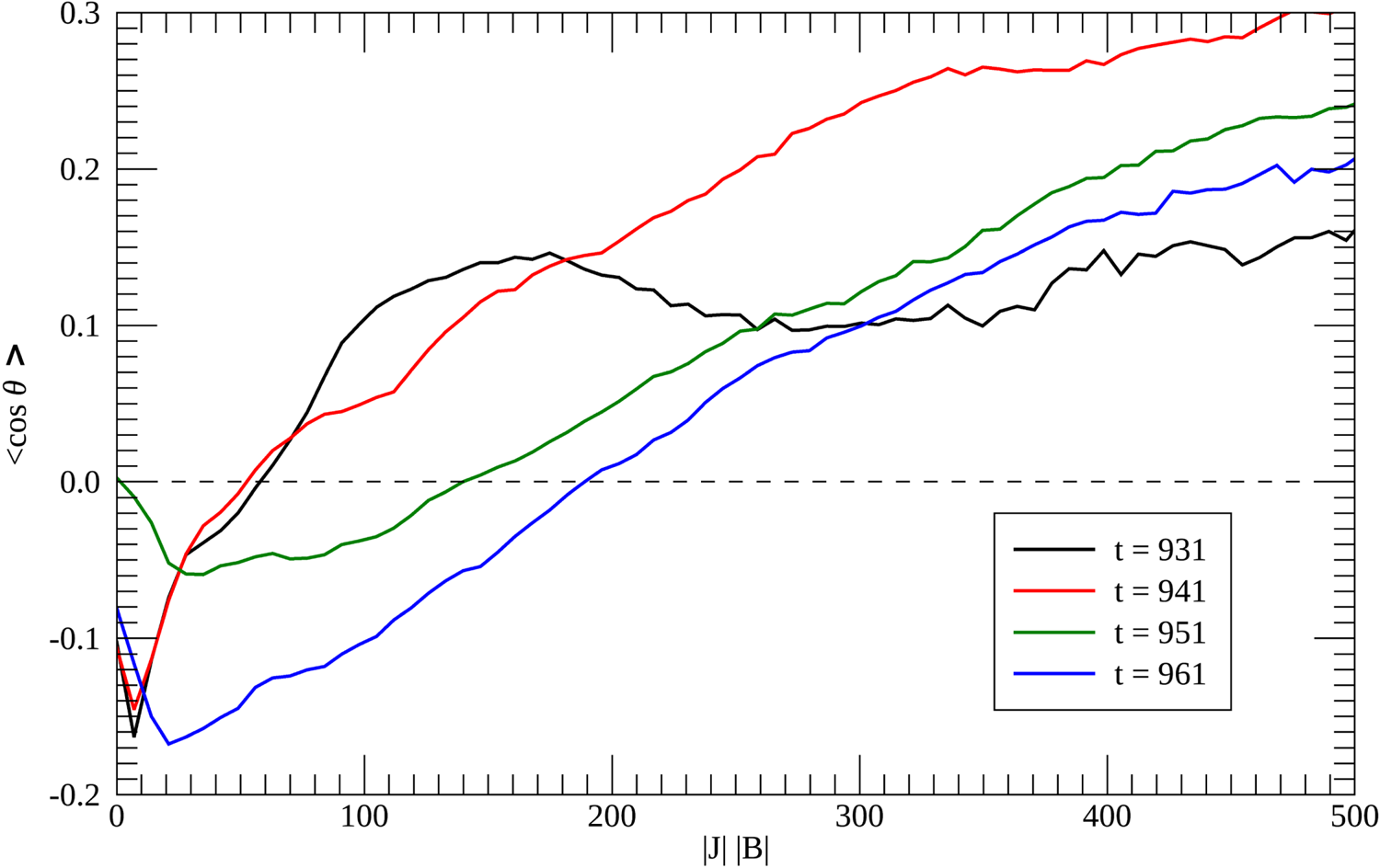
 $W_D$ is not driven by a corresponding abrupt decrease in either the current density or the magnetic field. These are both still near their peak values when the switching off takes place. Rather, the sudden decrease is brought about by a change in the alignment between fluctuations in
 $\boldsymbol {J}$ and
 $\boldsymbol {B}$. Figure 10 shows the average value of the cosine of the angle between
 $\boldsymbol {J}$ and
 $\boldsymbol {B}$ as a function of
 $|\boldsymbol {J}| |\boldsymbol {B}|$ at four different times: at the beginning of the pulse, just before the peak in
 $W_D$, just after the peak and after
 $W_D$ has decreased substantially. Keeping in mind that a large part of the contribution to
 $W_D$ comes from the small to moderate values of
 $|\boldsymbol {J}|$ and
 $|\boldsymbol {B}|$, we see that, even though overall the alignment is small, the rapid rise and rapid fall in
 $W_D$ is driven by first a slight increase in alignment followed by a slight increase in anti-alignment of these small to moderate values.
Plot of the helicity (black curve), of  $W_D$ (green curve) and of the sum of all the other terms on the right-hand side of (2.18) (red curve) as a function of time, for the pulse centred at
 $t=960$ The case is with
 $S=5$ moderate
 $Rm = 20$.

Average value of the cosine of the angle between  $\boldsymbol {J}$ and
 $\boldsymbol {B}$ as a function of
 $|\boldsymbol {J}| |\boldsymbol {B}|$ at four different times during the pulse centred at
 $t=960$, for the case with
 $S=5$ and moderate
 $Rm = 20$.

4. Conclusions
In this paper we have examined the effect of helicity flux on the generation of large-scale magnetic field for a model system at low Reynolds number and varying (low to moderate) magnetic Reynolds number. This approach has the advantage that, as  $Re$ is small, the flow is closely controlled by the imposed forcing. In particular, this means that the amount of helicity and the Lagrangian properties of the hydrodynamic flow can be selected relatively easily. However, the disadvantages include the fact that the flow is not really turbulent (although it may be chaotic) and so the dynamo dynamics may be constrained. This is not as limiting as one might expect. When the suppression of the turbulent alpha effect is discussed in the literature, the word turbulent refers to a lack of dependence on the diffusivity and not necessarily to a driving by a turbulent flow – a chaotic one will suffice. In this set-up, i.e. at low
 $Re$, a very strong field is produced with magnetic energy much larger than the kinetic energy (Brummell et al. Reference Brummell, Cattaneo and Tobias2001) and so large changes in the magnetic field are required to drive modest changes in the velocity. For this reason it is possible for the system to remain trapped in an invariant subspace (for example our high shear low
 $Rm$ case), with certain symmetry properties, where the dynamics may not be representative of more turbulent flows. Furthermore our choice of parameters mean that we are in the high
 $Pm$ regime.
For a dynamo system, conservation of helicity is not enforced. Indeed, breaking of helicity conservation is often crucial to the successful operation of the dynamo. For our system, a number of processes contribute to the evolution of magnetic helicity. Some involve diffusive processes (either volume terms or surface fluxes) and some remain even in the absence of diffusive terms. We find that the diffusive volume term ( $W_D$) always leads to the generation of helicity, whilst the rest of the terms, whether diffusive or ideal, (almost) always remove it. We find that two types of systematic field configurations may be generated, propagating dynamo waves and non-propagating mean fields. Our non-propagating cases have very little energy in the mean field components; open boundaries do not really help here.
An important result is that, for the case of strong shear we have investigated, the instantaneous diffusive volume term proportional to the current helicity decreases as  $Rm$ is increased. However, because the system undergoes oscillations, the time scale over which it acts is longer and so the integrated diffusive term remains similar. This is consistent with the diffusive term for magnetic helicity doing what is required to generate a large-scale field. However, the time scale needed for this term to operate effectively appears to scale with
 $Rm$. Hence it may take a diffusive time scale for the mean field to emerge if this is the only process of importance.
Clearly it will be necessary to extend these calculations to a much higher  $Rm$ to see which terms are asymptotically dominant. Previous calculations for dynamos where magnetic helicity is allowed to escape or enter the domain have produced results that are consistent with ours. These are interesting, though inconclusive. Dynamos in open domains do seem to produce fields with different characteristics to those in closed domains. For example, Hubbard & Brandenburg (Reference Hubbard and Brandenburg2010) found that, both the diffusive term and a helicity flux contribution to irreversibility decrease with increasing
 $Rm$. Linear extrapolation of their results indicates that the boundary term would dominate at sufficiently high
 $Rm$. Similar results have also been found by Sordo, Guerrero & Brandenburg (Reference Del Sordo, Guerrero and Brandenburg2013). In all cases examined, however, the ratio of mean field to fluctuating field continues to decrease with
 $Rm$ (Brandenburg Reference Brandenburg2018). For these models, as for ours, it is of significant interest to calculate the dynamics at higher
 $Rm$.
We conclude by stressing that, at least for these low and moderate values of  $Rm$, the large-scale dynamo does not seem to be constrained by helicity conservation, in the sense that there are plenty of terms that can effectively generate and remove helicity. Before embarking on extremely expensive calculations at high
 $Rm$ it may be appropriate to speculate on what to expect from such calculations. From the point of view of generation of large-scale flux the key property is that the turbulence should remain irreversible. In so far as irreversibility can be maintained the dynamo can continue to generate large-scale field. In a magnetised fluid irreversibility is associated either with reconnection, i.e. with the ability of the magnetic field to effectively change its topology, or with a flow of information out of the boundary. In principle, if the magnetofluid loses the ability to reconnect for dynamical reasons, it may still be able to maintain irreversibility through boundary terms. However, just because information could be lost through the boundary does not mean that it will. In this case open boundary conditions are a necessary though not sufficient condition for large-scale dynamo action. If, on the other hand, efficient reconnection can be maintained then open boundary conditions are not even necessary. Either way, the basic question is this: in a closed system, is it magnetic helicity conservation that drives the system towards reversibility by, say, removing the reconnection? Or is the conservation of helicity simply a manifestation of the loss of reconnection? We leave the reader with this thought. Magnetic helicity conservation in an ideal fluid follows from the induction equation alone and, as such, is a kinematic and not dynamical property. Loss of irreversibility is most likely associated with the dynamics and so we lean towards the latter possibility and not the former – but we keep an open mind.
Acknowledgements
S.M.T. is grateful to the Leverhulme Trust for the award of a Leverhulme Fellowship. G.B. acknowledges support from PRIN MIUR 2015 (grant no. 2015L5EE2Y).
Appendix A
In this appendix we describe how the vector function  $\boldsymbol {G}(x,z,t)$ used in the forcing is constructed.
 $\boldsymbol {G}(x,z,t)$ is the superposition of individual cellular forcings, i.e.
 \begin{equation} \boldsymbol{G}(x,z,t) = \sum_{\substack{{\boldsymbol k}\\6 \le k \le 8}} \boldsymbol{G}_{\boldsymbol{k}}(x,z,t), \end{equation}
where  $k=|{\boldsymbol k}|$ and each
 $\boldsymbol {G}_{\boldsymbol {k}}(x,z,t)$ is a cellular vector function on a scale
 $2 {\rm \pi} / k$. Each term in the sum,
 $\boldsymbol {G}_{\boldsymbol {k}}(x,z,t)$, is then computed from a single scalar function
 $\chi _{\boldsymbol {k}}$ so that
 ${g_{\boldsymbol {k}}}\boldsymbol {\cdot } \hat {\boldsymbol {x}}= -{\partial {\chi _{\boldsymbol {k}}}}/{\partial z}$ and
 ${g_{\boldsymbol {k}}} \boldsymbol {\cdot } \hat {\boldsymbol {z}} = {\partial \chi _{\boldsymbol {k}}}/{\partial x}$. To be clear what these functions look like we give the example for
 ${\boldsymbol k} =(5,0,6)$ then
 $\chi _{\boldsymbol {k}}$ has this form:
 \begin{equation} \chi_{\boldsymbol{k}} = A(\sqrt{61}) \exp \textrm{i} ( \theta_{\boldsymbol{k}}(t)+ 5 x) \sin 6z. \end{equation}
Clearly, if  $\chi _{\boldsymbol {k}}$ in phase space is given by a sine representation in
 $z$ then
 ${g_{\boldsymbol {k}}}\boldsymbol {\cdot }\hat {\boldsymbol {x}}$ and
 ${g_{\boldsymbol {k}}}\boldsymbol {\cdot }\hat {\boldsymbol {z}}$ satisfy the boundary conditions. With this choice, because
 $\chi _{\boldsymbol {k}}$ is independent of
 $y$,
 $\boldsymbol {G}_{\boldsymbol {k}}$ is automatically solenoidal. The construction of
 ${g_{\boldsymbol {k}}}\boldsymbol {\cdot } \hat {\boldsymbol {y}}$ requires a little care. In general, it is important to have a strongly helical forcing as this will (hopefully) engender a strongly helical flow. Ideally, that can be achieved by selecting
 ${g_{\boldsymbol {k}}} \boldsymbol {\cdot } \hat {\boldsymbol {y}} \sim k \chi _{\boldsymbol {k}}$, where
 $k$ is related to the wavenumber. However, this particular choice gives a
 ${g_{\boldsymbol {k}}} \boldsymbol {\cdot } \hat {\boldsymbol {y}}$ that does not satisfy the same boundary condition as
 $v$. This can be fixed by the following procedure. First the function
 $\chi _{\boldsymbol {k}}$ is transformed into configuration space using a sine transform. Then it is transformed back into phase space by a cosine transform. This generates a new function
 $\tilde {\chi }_{\boldsymbol {k}}$ that looks like the original function
 $\chi _{\boldsymbol {k}}$ except near the boundaries in
 $z$ where the derivative vanishes. In general, the cosine representation of a sine function contains a lot of high spatial frequencies which are mostly required to describe the very thin boundary layer over which the derivative goes to zero. For our purposes, we do not really require a thin boundary layer, and so we regularise
 $\tilde {\chi }_{\boldsymbol {k}}$ by only keeping the lowest
 $1/3$ of the wavenumbers. With this recipe the resulting forcing satisfies the boundary conditions and is close to being maximally helical.
In general we would like each  $\boldsymbol {G}_{\boldsymbol {k}}(t)$ to be a random function of time with a correlation time that can be adjusted to taste. This is achieved by the following method. The scalar function
 $\chi _{\boldsymbol {k}}$ is defined in phase space by a series of complex Fourier coefficients. The amplitude of these coefficients is only a function of
 $k$, while the phases are randomised by adding at every time step a small phase shift,
 $\delta ({\boldsymbol k})$, taken from a uniform distribution with
 $|\delta ({\boldsymbol k})| \le \delta _{\textrm {max}}({k})$ and
 $\delta _{\textrm {max}}({k})$ is chosen in such a way that in
 $N^2$ steps the phase will on average change by a fraction
 $c$ of
 $2 {\rm \pi}$. Here
 $N({k})$ is the number of time steps in a turnover time at scale
 $1/k$. Clearly
 $c=0$ corresponds to a steady flow, whilst
 $c \sim 1$ gives a forcing whose correlation time is similar to the turnover time.