1. Introduction
Efficient turbulent heat transfer enhancement with minimum momentum transfer enhancement is one of the outstanding problems to improve the performance of thermal devices, such as heat exchangers and cooling devices, with a small pumping power to drive the working fluid. However, dissimilar control of heat and momentum transfer is challenging because heat transfer enhancement is generally accompanied by momentum enhancement owing to the inherent similarity between the governing equations for the passive scalar and velocity fields. This was first noted by Reynolds (Reference Reynolds1874) and is known as the Reynolds analogy: the heat transfer rate is correlated with frictional resistance within the turbulent boundary layer for incompressible fluid. For smooth-wall-bounded turbulent flows, the similarity hypothesis also holds true for the mean velocity and temperature profiles (Kasagi, Tomita & Kuroda Reference Kasagi, Tomita and Kuroda1992; Pirozzoli, Bernardini & Orlandi Reference Pirozzoli, Bernardini and Orlandi2016), whereas dissimilarity appears in the higher-order moments of the fluctuation and derivative components (Abe & Antonia Reference Abe and Antonia2009, Reference Abe and Antonia2017; Takahashi et al. Reference Takahashi, Inagaki, Tsujimoto and Ando2025). This originates from the different natures of the velocity and temperature fields: velocity is a solenoidal vector field subject to the pressure gradient, whereas temperature is a scalar field. More importantly, flow manipulation potentially magnifies the effects of the different natures of the velocity and temperature fields, leading to the breakdown of the Reynolds analogy.
One of the most successful dissimilar heat transfer control techniques that achieves a favourable breakdown of the Reynolds analogy, that is, an increased heat transfer rate that is greater than the frictional resistance, is the travelling-wave-like local blowing/suction from the wall (Kong, Choi & Lee Reference Kong, Choi and Lee2001; Hasegawa & Kasagi Reference Hasegawa and Kasagi2011; Yamamoto, Hasegawa & Kasagi Reference Yamamoto, Hasegawa and Kasagi2013; Kaithakkal, Kametani & Hasegawa Reference Kaithakkal, Kametani and Hasegawa2020). These authors investigated the effects of local blowing/suction from the wall in a turbulent channel flow under specific thermal and flow conditions, which gives the same non-dimensional transport equations for the heat and momentum transfer. Kaithakkal et al. (Reference Kaithakkal, Kametani and Hasegawa2020) concluded that the modification of random components of the fluctuations by travelling-wave-like local blowing/suction increases the turbulent heat flux more than the Reynolds shear stress, resulting in considerable heat transfer rate enhancement relative to the increase in frictional resistance. Budget term analysis highlighted the important role of pressure fluctuations in the dissimilar transport mechanisms between the turbulent heat flux and Reynolds shear stress.
A favourable breakdown of the Reynolds analogy has also been achieved by wall manipulation techniques such as travelling-wave-like wall deformation (Uchino, Mamori & Fukagata Reference Uchino, Mamori and Fukagata2017) and spanwise wall oscillation (Guérin et al. Reference Guérin, Flageul, Cordier, Grieu and Agostini2024; Rouhi, Hultmark & Smits Reference Rouhi, Hultmark and Smits2025). Uchino et al. (Reference Uchino, Mamori and Fukagata2017) reported that a short-wavelength wall deformation with a large amplitude enhanced the heat transfer coefficient more than the skin friction coefficient by 13 %, whereas a somewhat smaller value of 6 % was achieved by wall oscillation (Guérin et al. Reference Guérin, Flageul, Cordier, Grieu and Agostini2024). Rouhi et al. (Reference Rouhi, Hultmark and Smits2025) reported that dissimilar reductions in the heat and momentum transfer could be achieved by spanwise wall oscillation, although the extent of the dissimilarity depends strongly on the forcing frequency and Prandtl number. Guérin et al. (Reference Guérin, Flageul, Cordier, Grieu and Agostini2024) attributed the favourable breakdown of the Reynolds analogy to the drag-increase phase of the wall oscillation, which led to a greater enhancement of the turbulent heat flux compared with the Reynolds shear stress. They also reported a stronger correlation between the wall-normal velocity and temperature fluctuations than that between the wall-normal and streamwise velocity fluctuations, and emphasized the importance of the pressure term in the streamwise momentum equation in achieving the favourable breakdown of the Reynolds analogy.
The introduction of the body force is another route for reproducing efficient turbulent heat transfer enhancement. Several theoretical studies by Alben (Reference Alben2017) and Motoki, Kawahara & Shimizu (Reference Motoki, Kawahara and Shimizu2018) demonstrated optimal heat transfer control that maximizes the heat transfer rate using the minimum power input, although the optimal field is driven by the artificial body force, which is not feasible for realistic flows. Another feasible body force approach for a favourable breakdown of the Reynolds analogy in engineering heat and mass transfer applications was reported by Matsubara & Alfredsson (Reference Matsubara and Alfredsson1996), Pirozzoli et al. (Reference Pirozzoli, Bernardini, Verzicco and Orlandi2017) and Brethouwer (Reference Brethouwer2021). Brethouwer (Reference Brethouwer2021) performed a direct numerical simulation (DNS) of plane Couette and Taylor–Couette flows with system rotation and found that the Coriolis force acts strongly to reduce momentum transfer by decreasing the streamwise/azimuthal velocity fluctuations while affecting the heat/mass transfer less. A favourably dissimilar enhancement of heat transfer can be achieved by the buoyancy force in turbulent channel flows with unstable thermal stratification, where the buoyancy force mixes heat more effectively than the momentum (Pirozzoli et al. Reference Pirozzoli, Bernardini, Verzicco and Orlandi2017).
An easier means of enhancing the heat transfer is to create roughness on the walls. This approach does not require any energy input and is categorized as passive control. The wall roughness leads to a considerable enhancement in the heat transfer rate but unfavourably breaks the similarity between the momentum and heat transfer. That is, the increase in frictional resistance is larger than that of the heat transfer rate. This is supported by experimental data (Dipprey & Sabersky Reference Dipprey and Sabersky1963; Kays & Crawford Reference Kays and Crawford1993; Bons Reference Bons2002), theoretical analyses (Katoh, Choi & Azuma Reference Katoh, Choi and Azuma2000) and DNS results (Forooghi et al. Reference Forooghi, Stripf and Frohnapfel2018a ; MacDonald, Hutchins & Chung Reference MacDonald, Hutchins and Chung2019; Kuwata Reference Kuwata2021, Reference Kuwata2022b ; Garg et al. Reference Garg, Sahut, Tuneskog, Nogenmyr and Fureby2024). The unfavourable breakdown of the Reynolds analogy is attributed to the pressure drag caused by the roughness obstruction, which directly increases the frictional resistance but not the heat transfer rate (MacDonald et al. Reference MacDonald, Hutchins and Chung2019; Kuwata Reference Kuwata2021). Hence, a streamwise-aligned roughness that does not offer a pressure drag alleviates the unfavourable breakdown of the Reynolds analogy (Stalio & Nobile Reference Stalio and Nobile2003; Stroh et al. Reference Stroh, Schäfer, Forooghi and Frohnapfel2020) or even breaks down the Reynolds analogy in a favourable manner (Choi & Orchard Reference Choi and Orchard1997; Rouhi et al. Reference Rouhi, Endrikat, Modesti, Sandberg, Oda, Tanimoto, Hutchins and Chung2022; Kuwata Reference Kuwata2022a ). In other words, the Reynolds analogy factor, which is defined as the ratio of the Stanton number to the skin friction coefficient, is much larger than that for smooth-wall turbulence. Kuwata (Reference Kuwata2022a ) studied the favourably dissimilar heat transfer enhancement over streamwise-aligned ribs by exploiting the fact that Kelvin–Helmholtz (K–H) instability-induced turbulence mixes scalars more efficiently than momentum (Ghisalberti & Nepf Reference Ghisalberti and Nepf2005; Nepf & Ghisalberti Reference Nepf and Ghisalberti2008). The streamwise-aligned slender rib arrays proposed by Kuwata (Reference Kuwata2022a ) allow the development of relatively large-scale turbulence associated with the K–H instability, resulting in a considerably favourable breakdown of the Reynolds analogy. Rouhi et al. (Reference Rouhi, Endrikat, Modesti, Sandberg, Oda, Tanimoto, Hutchins and Chung2022) also achieved the favourable breakdown of the Reynolds analogy by the riblet grooves. Rouhi et al. (Reference Rouhi, Endrikat, Modesti, Sandberg, Oda, Tanimoto, Hutchins and Chung2022) attributed this to the negative wall shear stress within the riblet grooves, which is induced by spanwise rollers associated with the K–H instability. Because there is no corresponding negative counterpart in the heat transfer coefficient, this effect reduces only the frictional resistance. Kuwata (Reference Kuwata2022a ) and Rouhi et al. (Reference Rouhi, Endrikat, Modesti, Sandberg, Oda, Tanimoto, Hutchins and Chung2022) concluded that turbulence plays a dominant role in the favourable breakdown of the Reynolds analogy, whereas secondary flows induced by the roughness act to diminish this effect.
Kuwata (Reference Kuwata2022a
) achieved a significant favourable breakdown of the Reynolds analogy: the enhancement of the heat transfer coefficient exceeded the increase in the skin friction coefficient by 40 %. However, Kuwata (Reference Kuwata2022a
) considered only a single friction Reynolds number of
 $\textit{Re}_\tau = 300$
, which makes it difficult to discuss the scaling of heat transfer characteristics. Moreover, their study primarily focused on the emergence of dissimilar heat transfer induced by the K–H instability and did not provide sufficient statistical evidence for the physical mechanisms underlying the favourable breakdown of the Reynolds analogy. In particular, the importance of pressure in the dissimilar heat transfer was suggested by Kuwata (Reference Kuwata2022a
) and Guérin et al. (Reference Guérin, Flageul, Cordier, Grieu and Agostini2024); however, the detailed processes by which pressure contributes to the favourable breakdown of the Reynolds analogy remain unclear. The present study extends the work of Kuwata (Reference Kuwata2022a
) by investigating both the Reynolds number effects and the physical mechanisms responsible for the breakdown of the Reynolds analogy. We consider heat transfer conditions identical to those in Kuwata (Reference Kuwata2022a
), while additionally performing simulations at lower and higher friction Reynolds numbers of
 $\textit{Re}_\tau = 180$
and
 $\textit{Re}_\tau = 500$
, respectively. We elucidate the scaling of the modifications in the mean velocity, mean temperature, Reynolds analogy factor and the characteristic wavelength and intensity of the K–H instability. In addition, we examine in detail the mechanisms responsible for the favourable breakdown of the Reynolds analogy from two perspectives: (i) instantaneous and local dissimilar heat transfer characteristics, and (ii) transport mechanisms of turbulent heat and momentum fluxes.
2. The DNS methodology
2.1. Flow conditions
Although the flow geometry was identical to that in our previous study (Kuwata Reference Kuwata2022a
), we briefly explain the flow conditions for the sake of completeness. We considered a turbulent open-channel flow over streamwise-aligned longitudinal slender rib arrays, as illustrated in figure 1. The computational domain lengths in the streamwise (
 $x$
) and spanwise (
 $z$
) directions were
 $L_x$
and
 $L_z$
, respectively, and
 $H$
was the channel height in the clear flow region (
 $y\gt 0$
). The streamwise-aligned longitudinal ribs were mounted regularly on the base wall, whereas slip boundary conditions were imposed on the top boundary face. As opposed to previous studies on longitudinal rib roughness (Orlandi, Leonardi & Antonia Reference Orlandi, Leonardi and Antonia2006; Stroh et al. Reference Stroh, Schäfer, Forooghi and Frohnapfel2020), the height of the current rib arrays
 $h$
was comparable to the channel height
 $H$
, that is,
 $h=H/1.5$
, which allowed turbulent fluctuations associated with K – H instability to develop (Kuwata Reference Kuwata2022a
). The flow was periodic in the
 $x$
- and
 $z$
-directions, and a pressure difference was prescribed in the
 $x$
-direction to drive the flow. The friction Reynolds number for the clear flow region (
 $0\lt y\lt H$
) was fixed at
 $\textit{Re}_\tau =u_\tau H/\nu =180$
and
 $500$
, where
 $u_\tau$
is the average friction velocity at the rib crest (
 $y=0$
) and
 $\nu$
is the kinematic viscosity. We include the DNS results at
 $\textit{Re}_\tau =300$
from Kuwata (Reference Kuwata2022a
) in the following discussion. We considered an incompressible fluid and a passive scalar with a molecular Prandtl number
 $\textit{Pr}=1$
. The buoyancy effects and temperature dependence of the physical properties were neglected. The top boundary face was adiabatic, whereas a constant temperature was specified at the surfaces of the ribs and base wall. The heat transfer was driven by the volumetric heat generation
 $q_v$
, which was cooled by the ribs and base wall. In this set of heat transfer and fluid flow conditions, the streamwise momentum and heat transport equations in a non-dimensional form are similar (Kasagi et al. Reference Kasagi, Hasegawa, Fukagata and Iwamoto2010; Hasegawa & Kasagi Reference Hasegawa and Kasagi2011),
 \begin{eqnarray} \frac {\partial u^+}{\partial t^+} + u^+_{\!j} \frac {\partial u^+}{\partial x_{\!j}^+} &=& 1 + \frac {\partial }{\partial x_{\!j}^+} \left ( \frac {\partial u^+}{\partial x_{\!j}^+}\right )-\frac {\partial p^{\prime^+}}{\partial x^+}, \end{eqnarray}
 \begin{eqnarray} \frac {\partial \theta ^+}{\partial t^+} + u^+_{\!j}\frac {\partial \theta ^+}{\partial x_{\!j}^+} &=& 1 + \frac {1}{\textit{Pr}}\frac {\partial }{\partial x_{\!j}^+} \left ( \frac {\partial \theta ^+}{\partial x_{\!j}^+}\right ), \end{eqnarray}
where
 $u$
is the streamwise velocity component,
 $\theta =T-T_w$
is the relative temperature and
 $p^\prime=p-\overline {p}$
is the pressure fluctuation. An overbar denotes averaging in the time and homogeneous directions, whereas a prime denotes its fluctuation. The inner-scaled quantities normalized by the friction velocity
 $u_\tau$
or friction temperature
 $\theta _\tau$
are marked with a superscript ‘+’. When
 $\textit{Pr}=1$
, the non-dimensional transport equations for
 $u$
and
 $\theta$
are similar except for the pressure fluctuation term on the right-hand side of (2.1).
Computational geometry of the longitudinal rib-roughened open-channel flows. Here,
 $H$
is the clear channel height,
 $h$
is the rib height,
 $s$
is the separation between the ribs and
 $w$
is the thickness of the rib. The streamwise and spanwise domain lengths are
 $L_x$
and
 $L_z$
, respectively.

The friction velocity
 $u_\tau$
is given by the wall shear stress
 $\tau _w$
, which is equivalent to the total shear stress at the rib crest position (
 $y=0$
) and is balanced by the mean pressure gradient in the clear flow region, as follows:
 \begin{equation} \tau _w/\rho = u_\tau ^2 = -\frac {1}{\rho } \frac {\partial \overline {p}}{\partial x}H, \end{equation}
where
 $\rho$
is the density. Analogously, the friction temperature
 $\theta _\tau$
is given by the wall heat flux
 $q_w$
, which is equivalent to the total heat flux at the rib crest and is balanced by the total amount of heat generation in the clear flow region (
 $0\lt y\lt H$
), as follows:
 \begin{equation} q_w = \rho c u_\tau \theta _\tau = q_vH, \end{equation}
where
 $c$
is the specific heat.
Parameters of the DNS and rib arrays: friction Reynolds number
 $\textit{Re}_\tau =u_\tau H/\nu$
, spanwise separation between the ribs
 $s$
, thickness of a rib
 $w$
, permeability of finite parallel rib arrays
 $K_\infty$
, permeability Reynolds number
 $\textit{Re}_K=\sqrt {K_\infty }/\ell _v$
and square root of the groove cross-section
 $\ell _g = \sqrt {sh}$
. The information for case 300 was obtained from Kuwata (Reference Kuwata2022a
).

2.2. Rib arrays
The geometry of the streamwise-aligned longitudinal rib arrays was identical to that in the previous study (Kuwata Reference Kuwata2022a
). The rib thickness was fixed at
 $w=0.05h$
, resulting in an aspect ratio of
 $h/w=20$
. In addition to the reference smooth-wall simulations, we considered five cases with different separations between the ribs:
 $s/h=0.05, 0.075, 0.2, 0.45$
and
 $1.2$
, which yielded a considerable variation in permeability within the rib array regions. The permeability
 $K_\infty$
quantifies the ease of flow within the rib array regions in
 $y\lt 0$
, which is defined by Darcy’s law (Whitaker Reference Whitaker1986),
 \begin{equation} U_d = -\frac {K_\infty }{\mu }\frac {\partial p}{\partial x}, \end{equation}
where
 $U_d$
is the Darcian velocity and
 $\mu$
is the fluid viscosity. The permeability
 $K_\infty$
of the current rib arrays can be analytically derived by assuming fully developed laminar flows bounded by two infinite parallel walls,
 \begin{equation} K_\infty = \frac {1}{12}\frac {s}{s+w}s^2. \end{equation}
The different separations between the ribs yielded variations in
 $K_\infty /H^2$
from
 $4.6 \times 10^{-4}$
to
 $5.1 \times 10^{-2}$
. The flow conditions and parameters related to the rib array geometry are listed in table 1. Each case is labelled R-P; the first letter ‘R’ indicates the nominal friction Reynolds number, and the latter one ‘P’ indicates a volume percentage of fluid phase within the rib region, i.e.
 $100\times \varphi$
[%], where the porosity is
 $\varphi =s/(s+w)$
. Table 1 shows the length scales of the rib arrays normalized by the inner length scale
 $\ell _v=\nu /u_\tau$
, such as the permeability Reynolds number
 $\textit{Re}_K=\sqrt {K_\infty }/\ell _v$
, spanwise separation between the ribs
 $s^+=s/\ell _v$
and rib height
 $h^+=h/\ell _v$
. Following the classification provided by Breugem, Boersma & Uittenbogaard (Reference Breugem, Boersma and Uittenbogaard2006) based on the permeability Reynolds number
 $\textit{Re}_K$
, the present simulations covered the partially permeable regime
 $\textit{Re}_K \simeq 1$
, where the permeability substantially affects turbulent flows and goes beyond the highly permeable regime
 $\textit{Re}_K\gt 10$
in which the viscous effects are of minor importance. Considering the criterion for drag-reducing riblet surfaces of
 $s^+\lt 30$
(Bechert et al. Reference Bechert, Bruse, Hage, Van der Hoeven and Hoppe1997), drag reduction is expected for the current rib arrays. However, this does not necessarily occur because the square root of the groove cross-section
 $\ell _g^+ = \sqrt {sh}^+$
is significantly larger than the threshold value for the drag-increasing riblet surfaces of
 $\ell ^+_g \simeq 11$
, above which spanwise roller vortices owing to K–H instability develop over the groove roughness (Garcia-Mayoral & Jiménez Reference Garcia-Mayoral and Jiménez2011; Endrikat et al. Reference Endrikat, Modesti, MacDonald, García-Mayoral, Hutchins and Chung2021b
).
2.3. Numerical set-up
For the numerical method, we used the double population distribution function lattice Boltzmann method (LBM), in which the time evolutions of the lattice Boltzmann equations for the particle density and energy distribution functions are solved for the velocity and temperature fields, respectively. There are several possible choices for the collision and discrete velocity models in the LBM. In this study, we selected the 27-velocity multiple-relaxation-time LBM (Suga et al. Reference Suga, Kuwata, Takashima and Chikasue2015) for the velocity fields and 19-velocity regularized LBM (Suga, Chikasue & Kuwata Reference Suga, Chikasue and Kuwata2017a
) for the temperature fields. The validity of the LBM–DNS for turbulent flows was established by comparing the experimental data for a duct with partially filled rod arrays (Kuwata, Tsuda & Suga Reference Kuwata, Tsuda and Suga2020), the DNS results for sinusoidal roughness (Kuwata, Yagasaki & Suga Reference Kuwata, Yagasaki and Suga2024) and turbulent channel, pipe and duct flows (Suga et al. Reference Suga, Kuwata, Takashima and Chikasue2015). The LBM employs an evenly spaced regular grid system. The grid resolution adheres to the well-established guidelines in Suga et al. (Reference Suga, Kuwata, Takashima and Chikasue2015) that the near-wall grid spacing for the LBM–DNS should be approximately
 $\varDelta ^+ \simeq 1.8$
, where
 $\varDelta ^+$
denotes the grid spacing in the wall unit. For the current DNS, to circumvent the high cost of simulating an entire domain using a single-resolution mesh, we used the two-level hierarchical grid refinement method of Kuwata & Suga (Reference Kuwata and Suga2016), with which we allocated twice coarser grid away from the rib roughness at
 $y^+\simeq 60$
(case 180) and
 $y^+\simeq 90$
(case 500). The size of the computational domain was comparable to that in the previous DNS case (case 300) from Kuwata (Reference Kuwata2022a
). However, the domain lengths of the current DNS cases (cases 180 and 500) were slightly extended in the streamwise and spanwise directions. The spanwise domain length was
 $L_z=5H$
and the streamwise domain lengths were
 $L_x=8H$
for case 180 and
 $L_x=6H$
for case 500. In the presence of the K–H instability within the computational domain, the domain size should be sufficiently large to accommodate the streamwise perturbations associated with the K–H instability. A viscous scaling has been proposed for the characteristic streamwise length scale of the K–H instability over drag-increasing riblets (Garcia-Mayoral & Jiménez Reference Garcia-Mayoral and Jiménez2011; Endrikat et al. Reference Endrikat, Modesti, García-Mayoral, Hutchins and Chung2021a
). These studies found approximate values of
 $\lambda _x^+ \simeq 150$
for blade riblets (Garcia-Mayoral & Jiménez Reference Garcia-Mayoral and Jiménez2011) and
 $\lambda _x^+ \simeq 180$
for triangular and blade-shaped riblets (Endrikat et al. Reference Endrikat, Modesti, García-Mayoral, Hutchins and Chung2021a
). In contrast, the experiments over a wide range of Reynolds numbers and permeabilities conducted by Suga et al. (Reference Suga, Nakagawa and Kaneda2017b
) showed that the length scale was several times larger than the boundary layer thickness,
 $3.4\lt \lambda _x/\delta \lt 5.5$
, where
 $\delta$
denotes the boundary-layer thickness. This scaling was further supported by the results of a DNS of a high-porosity foam matrix (
 $3\lt \lambda _x/\delta \lt 5$
) performed by Kuwata & Suga (Reference Kuwata and Suga2024). Although the scaling of the spatial extent of the K–H instability is discussed in § 3.2, it can be inferred that the present streamwise domain length (
 $L_x/H=8$
,
 $L_x^+=1430$
at
 $\textit{Re}_\tau =180$
;
 $L_x/H=6$
,
 $L_x^+=2680$
at
 $\textit{Re}_\tau =500$
) is sufficiently larger than the characteristic length scale of the K–H-induced streamwise perturbation from both the viscous-scaling (
 $150 \lesssim \lambda _x^+ \lesssim 180$
; Garcia-Mayoral & Jiménez (Reference Garcia-Mayoral and Jiménez2011) and Endrikat et al. (Reference Endrikat, Modesti, García-Mayoral, Hutchins and Chung2021a
)) and outer-scaling perspectives (
 $3 \lesssim \lambda _x/H \lesssim 5.5$
; Suga et al. (Reference Suga, Nakagawa and Kaneda2017b
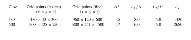
) and Kuwata & Suga (Reference Kuwata and Suga2024)). Further discussion on the characteristic wavelength is provided in § 3.2 and validation results verifying the grid resolution and domain size are provided in Appendix A. The parameters related to the numerical set up are shown in table 2.
Regarding the vertical extent of the computational domain, slip boundary conditions were imposed on the top boundary, following the author’s previous study (Kuwata Reference Kuwata2022a ). The non-penetration constraint at the boundary may affect the development of turbulence structures associated with the K–H instability when their length scale is of the same order as the channel height. Other possible flow configurations include a channel bounded by two porous/rough walls (Sharma Reference Sharma and García-Mayoral2020; Rouhi et al. Reference Rouhi, Endrikat, Modesti, Sandberg, Oda, Tanimoto, Hutchins and Chung2022), and a channel with one porous/rough wall and one smooth wall (Breugem et al. Reference Breugem, Boersma and Uittenbogaard2006; Suga et al. Reference Suga, Matsumura, Ashitaka, Tominaga and Kaneda2010). However, it remains unclear how these different flow configurations influence the large-scale motions associated with the K–H instability. Therefore, for simplicity, an open-channel flow configuration was adopted in the present study, following the author’s previous study (Kuwata Reference Kuwata2022a ).
2.4. Averaging procedure
As in flows over porous/rough walls, where the time mean velocity is not homogeneous in the
 $x{-}z$
plane, we discuss the mean profiles averaged over time and space (
 $x{-}z$
plane). The time-averaged value of a variable
 $\phi$
is denoted by
 $\overline {\phi }$
, and
 $\phi ^\prime$
denotes the fluctuation from the Reynolds-averaged value:
 $\phi ^\prime = \phi -\overline {\phi }$
. In addition, the superficial spatial averaging of the variable
 $\phi$
in the
 $x{-}z$
plane is introduced as follows:
 \begin{equation} {\langle \phi \rangle }(y,t) = \frac {1}{L_xL_z}\int _{x_{\!f}} \int _{z_{\!f}} \phi (x,y,z,t) {\rm d}x{\rm d}z, \end{equation}
where
 $x_{\!f}$
and
 $z_{\!f}$
denote the positions in the fluid phase. The deviation from the fluid phase spatial averaging,
 ${\langle \phi \rangle }/\varphi$
, is defined as a dispersion:
 $\tilde {\phi } = \phi -{\langle \phi \rangle }/\varphi$
, where
 $\varphi$
is the
 $x{-}z$
plane porosity. Note that the order of the spatial and Reynolds averaging operators are interchangeable (Pedras & de Lemos Reference Pedras and de Lemos2000). For Reynolds averaging, the statistics were accumulated over approximately
 $100H/u_\tau$
for the cases at
 $\textit{Re}_\tau =180$
and
 $50H/u_\tau$
for the cases at
 $\textit{Re}_\tau =500$
.
Parameters related to the numerical set-up. Here,
 $\varDelta ^+=\varDelta /\ell _v$
is the inner-scaled grid spacing for the fine grid block,
 $L_x$
is the streamwise domain length and
 $L_z$
is the spanwise domain length.

3. Results and discussion
3.1. Mean profiles
Figure 2 shows the inner-scaled mean velocity
 $U^+={\langle \overline {u}\rangle }^+$
and temperature
 $\varTheta ^+={\langle \overline {\theta }\rangle }^+$
profiles. As expected, the mean velocity and temperature within the rib array region (
 $y\lt 0$
) increase with the volume fraction
 $\varphi$
of the fluid phase below the rib crest. This is a direct result of an increase in the permeability
 $K_{\infty }$
with
 $\varphi$
. However, the modifications of
 $U^+$
and
 $\varTheta ^+$
in the clear flow region (
 $y\gt 0$
) are not monotonic:
 $U^+$
and
 $\varTheta ^+$
decrease with
 $\varphi$
from 0.5 to 0.8, whereas a further increase in
 $\varphi$
increases them. The reduction in the
 $U^+$
and
 $\varTheta ^+$
profiles in the clear flow region exhibits a strong
 $\textit{Re}_\tau$
dependency for the case with
 $\varphi =0.5$
. Specifically, for the dense rib array with
 $\varphi =0.5$
, the
 $U^+$
and
 $\varTheta ^+$
profiles at
 $\textit{Re}_\tau =180$
(case 180-0.5) in figure 2(a) are almost unaffected by the rib array, whereas the dense rib array at
 $\textit{Re}_\tau =500$
(case 500-0.5) in figure 2(d) exhibits a notable reduction in the
 $U^+$
and
 $\varTheta ^+$
profiles. Another notable observation is that the effects of the rib array on
 $U^+$
and
 $\varTheta ^+$
differ significantly. Because the Reynolds analogy holds for the smooth-wall case at
 $\textit{Pr}=1$
, the
 $U^+$
and
 $\varTheta ^+$
profiles collapse onto one another at
 $\textit{Re}_\tau =180$
and
 $500$
. In contrast, the rib arrays decrease the
 $\varTheta ^+$
profiles more than the
 $U^+$
profiles. This trend is particularly pronounced in the clear flow region and is a sign of the breakdown of the Reynolds analogy by the rib arrays. This is consistent with the results at
 $\textit{Re}_\tau =300$
obtained from Kuwata (Reference Kuwata2022a
).
Inner-scaled mean velocity
 $U^+={\langle \overline {u}\rangle }^+$
and temperature
 $\varTheta ^+={\langle \overline {\theta }\rangle }^+$
profiles: (a,b,c)
 $\textit{Re}_\tau =180$
and (d,e, f)
 $\textit{Re}_\tau =500$
. The rib spacing, i.e. volume fraction
 $\varphi$
within the rib region, increases from left to right. The rib crest and base wall positions are
 $y/H=0$
and
 $y/H=-2/3$
, respectively. The solid and dashed lines indicate the temperature
 $\varTheta ^+$
and velocity
 $U^+$
, respectively.

Inner-scaled mean velocity
 $U^+$
profiles with (a,b) log–linear format and (c,d) defect form: (a,c)
 $\textit{Re}_\tau =180$
and (b,d)
 $\textit{Re}_\tau =500$
. The smooth-wall results from Kim, Moin & Moser (Reference Kim, Moin and Moser1987) at
 $\textit{Re}_\tau =180$
and from Lluesma-Rodríguez et al. (Reference Lluesma-Rodríguez, Hoyas and Perez-Quiles2018) at
 $\textit{Re}_\tau =500$
are included for comparison.

The profiles of
 $U^+$
are shown in a log–linear format in figure 3(a,b) and in defect form in figure 3(c,d). For comparison, the smooth-wall results from Kim et al. (Reference Kim, Moin and Moser1987) and Lluesma-Rodríguez et al. (Reference Lluesma-Rodríguez, Hoyas and Perez-Quiles2018) are included as a reference. As shown in figure 3(a,b), the current smooth-wall results are in excellent agreement with the reference DNS data. The minor difference between the current and reference DNS results may be attributed to differences in the flow configurations. The current DNS is for open-channel flows, whereas the reference DNS was for full-channel flows bounded by two parallel walls. As shown in figure 3(a,b), the slopes of the
 $U^+$
profiles away from the rib arrays are not significantly different from the smooth-wall results, despite the significant increase in
 $U^+$
near the rib arrays for cases with
 $\varphi =0.9$
and
 $0.96$
. The similarity in the slopes of the
 $U^+$
profiles is evident in the defect forms shown in figure 3(c,d). The similarity in terms of
 $U^+$
is almost perfect at
 $\textit{Re}_\tau =180$
, except for case 180-0.8 (figure 3
c), but becomes marginally worse at
 $\textit{Re}_\tau =500$
(figure 3
d). Although the results are not shown here, a similarity away from the rib arrays is observed for the
 $\varTheta ^+$
profiles. A more detailed description of the similarity can be found in Appendix B.
(a,c) Velocity roughness functions
 $\Delta U^+$
and (b,d) temperature roughness function
 $\Delta \varTheta ^+$
: (a,b) against the permeability Reynolds number
 $\textit{Re}_K=\sqrt {K_\infty }^+$
and (c,d) against the Darcy number
 $\sqrt {Da}=\sqrt {K_\infty }/H$
. The thin lines in the figure are the approximate lines that indicate the trend of
 $\Delta U^+$
or
 $\Delta \varTheta ^+$
. The results at
 $\textit{Re}_\tau =300$
were obtained from Kuwata (Reference Kuwata2022a
).

The persistent similarity in
 $U^+$
and
 $\varTheta ^+$
away from the rib arrays allows us to define the velocity and temperature roughness functions
 $\Delta U^+$
and
 $\Delta \varTheta ^+$
, respectively. The roughness functions
 $\Delta U^+$
and
 $\Delta \varTheta ^+$
were defined as the downward shift values in
 $U^+$
and
 $\varTheta ^+$
with respect to the corresponding smooth-wall profiles, which were evaluated at
 $y^+\simeq 90$
(
 $\textit{Re}_\tau =180$
) and
 $y^+\simeq 250$
(
 $\textit{Re}_\tau =500$
) in this study. See Appendix B for the uncertainty in the evaluation for the roughness function. The concept of
 $\Delta U^+$
originates from an experimental study on rough-wall turbulence (Schlichting Reference Schlichting1937) and is commonly used in the context of rough-wall turbulence to quantify the increase in momentum transfer owing to wall roughness. In this study, we used
 $\Delta U^+$
and
 $\Delta \varTheta ^+$
to measure the effects of the rib arrays on the
 $U^+$
and
 $\varTheta ^+$
profiles, respectively. Note that the imperfect similarity in the
 $U^+$
profiles in the logarithmic region may cause uncertainty in estimating
 $\Delta U^+$
. However, we confirmed that the uncertainty of
 $\Delta U^+$
arising from the different evaluation locations was small (less than 3.1 % at
 $\textit{Re}_\tau =500$
; see Appendix B).
Figure 4 plots the roughness functions against the permeability Reynolds number
 $\textit{Re}_K$
in figure 4(a,b) and Darcy number
 $\sqrt {Da}=\sqrt {K_\infty }/H$
in figure 4(c,d). Note that the square root of the permeability is expressed as
 $\sqrt {K_\infty }=\sqrt {\varphi /12} \ s$
from the definition of
 $K_\infty$
in (2.6). Hence,
 $\textit{Re}_K=\sqrt {\varphi /12} \ s^+$
and
 $\sqrt {Da}=\sqrt {\varphi /12} \ s/H$
are related to the inner- and outer-scaled separation between the ribs, respectively. We observe from figure 4(a,b) that the roughness functions increase with
 $\textit{Re}_K$
up to
 $\textit{Re}_K \simeq 20$
, although a further increase in
 $\textit{Re}_K$
decreases the roughness functions. In the decreasing region, the roughness functions are not expressed as functions of
 $\textit{Re}_K$
but could be scaled by the Darcy number
 $\sqrt {Da}$
, as shown in figure 4(c,d). Notably, the trend of
 $\Delta U^+$
is significantly different from that observed in rough- or porous-wall turbulence, where
 $\Delta U^+$
increases progressively with the inner-scaled roughness length in the fully rough regime (Schlichting Reference Schlichting1937; Flack & Schultz Reference Flack and Schultz2010; Okazaki et al. Reference Okazaki, Shimizu, Kuwata and Suga2020). This is because of the absence of pressure drag in streamwise-aligned rib arrays because the pressure drag plays a dominant role in increasing the wall resistance in the fully rough regime (Scaggs, Taylor & Coleman Reference Scaggs, Taylor and Coleman1988). However, the importance of
 $\textit{Re}_K$
in the earlier stages of the emergence of rib array effects in
 $\textit{Re}_K\lt 10$
is consistent with the observation of porous-wall turbulence by Suga et al. (Reference Suga, Matsumura, Ashitaka, Tominaga and Kaneda2010), who showed that
 $\textit{Re}_K$
is a good measure of the effects of wall permeability on turbulence for a moderate
 $\textit{Re}_K$
regime of
 $\textit{Re}_K \lt 3$
. Another important observation is that
 $\Delta \varTheta ^+$
generally exceeds
 $\Delta U^+$
, suggesting that the effect of the rib arrays on
 $\varTheta ^+$
is greater than that on
 $U^+$
.
Further implications from figure 4 can be obtained by considering that the roughness functions are related to the skin friction coefficient
 $C_{\!f}=2/(U_b^+)^2$
and Stanton number
 $S_t=1/(U_b^+ \varTheta _a^+)$
using the following relations (Aupoix Reference Aupoix2015):
 \begin{equation} \Delta U^+ = \sqrt {\frac {1}{0.5C_{\!f0}}}-\sqrt {\frac {1}{0.5C_{\!f}}}, \qquad \Delta \varTheta ^+=\frac {\sqrt {0.5C_{\!f0}}}{S_{t0}}-\frac {\sqrt {0.5C_{\!f}}}{S_{t}}, \end{equation}
where
 $C_{\!f0}$
and
 $S_{t0}$
are the corresponding values for smooth-wall turbulence at the same
 $\textit{Re}_\tau$
,
 $U_b$
is the bulk mean velocity and
 $\varTheta _a$
is the arithmetic mean temperature. Hence, the increasing trend of
 $\Delta U^+$
in figure 4(a) indicates an increase in
 $C_{\!f}$
with
 $\textit{Re}_K$
. In contrast, the
 $\textit{Re}_K$
independent value of
 $\Delta U^+$
for the sparse rib array cases with
 $\varphi =0.9$
and
 $0.96$
implies that the effect of
 $\textit{Re}_\tau$
on
 $C_{\!f}$
is similar to that for smooth-wall turbulence. A plausible explanation for this trend is that in the sufficiently large
 $\textit{Re}_K$
regime, a turbulent boundary layer is developed over each rib wall, where the frictional resistance exhibits a similar
 $\textit{Re}_\tau$
dependence to that of smooth-wall turbulence.
Augmentation of the Stanton number
 $S_t/S_{t0}$
against that of the skin friction coefficient
 $C_{\!f}/C_{\!f0}$
from smooth-wall turbulence at the same
 $\textit{Re}_\tau$
. The thin line is
 $S_t/S_{t0}=C_{\!f}/C_{\!f0}$
, which means that the Reynolds analogy factor
 $\textit{RA}$
is the same as that for the smooth-wall turbulence
 $\textit{RA}_0$
. The dashed line is the approximate line for the current results,
 $S_t/S_{t0} = (C_{\!f}/C_{\!f0})^{1.28}$
. The results at
 $\textit{Re}_\tau =300$
are from Kuwata (Reference Kuwata2022a
).

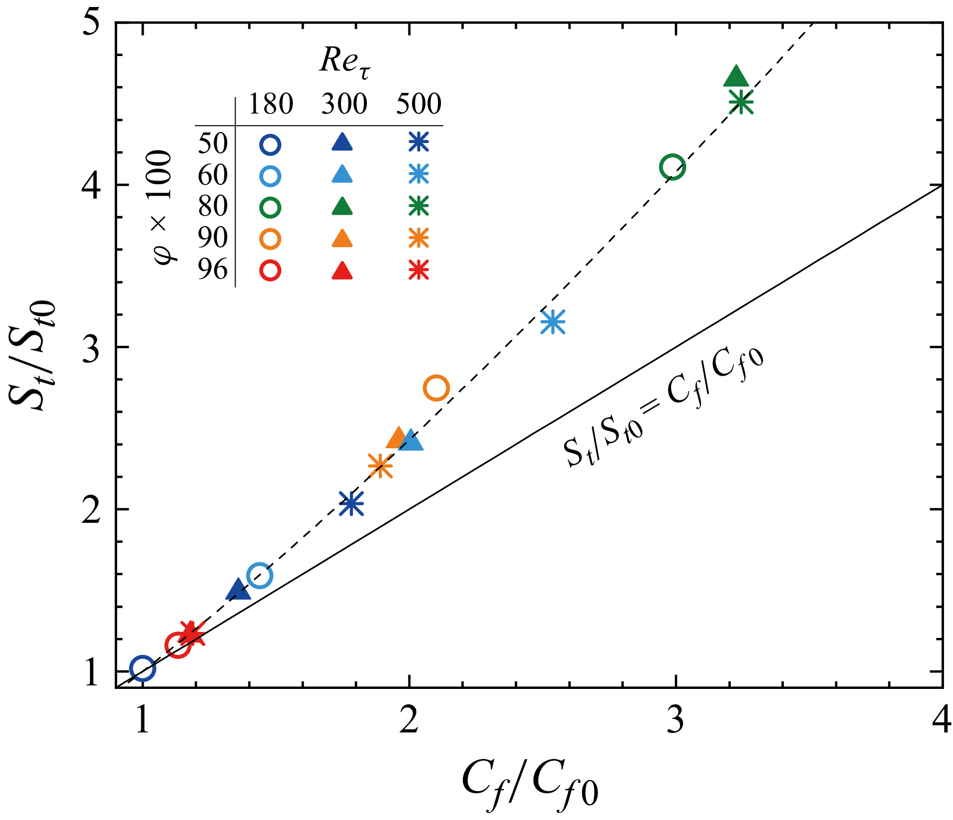
Figure 5 plots the augmentations of
 $C_{\!f}$
and
 $S_t$
owing to the rib arrays. The figure shows that the drag increase, that is,
 $C_{\!f}/C_{\!f0}\gt 1$
occurs for all current rib arrays despite the fact that some cases are within the drag reduction regime judging from the criteria based on
 $s^+$
(Bechert et al. Reference Bechert, Bruse, Hage, Van der Hoeven and Hoppe1997). This inconsistency is attributed to the significantly deep grooves of the current rib arrays, because the depth of the grooves is an important factor that affects the frictional drag (Garcia-Mayoral & Jiménez Reference Garcia-Mayoral and Jiménez2011). In the limit of dense rib arrays, where the rib arrays almost behave as a hydraulically smooth wall, that is,
 $C_{\!f}/C_{\!f0}\simeq 1$
, the results are asymptotic to the diagonal line
 $C_{\!f}/C_{\!f0} = S_t/S_{t0}$
. This indicates that the Reynolds analogy factor
 $\textit{RA}=2S_t/C_{\!f}$
is asymptotically close to the values for the smooth-wall turbulence
 $\textit{RA}_0=2S_{t0}/C_{\!f0}$
. However, the results start to deviate from the diagonal line as the augmentations of
 $C_{\!f}$
and
 $S_t$
became more significant. Interestingly, the results almost follow a single curve of
 $S_t/S_{t0} = (C_{\!f}/C_{\!f0})^{1.28}$
despite significant variations in
 $\textit{Re}_\tau$
and
 $\varphi$
. That is, the normalized Reynolds analogy factor
 $\textit{RA}/\textit{RA}_0$
increases with
 $C_{\!f}/C_{\!f0}$
, as follows:
 $\textit{RA}/\textit{RA}_0=(C_{\!f}/C_{\!f0})^{0.28}$
. Note that the trend of the current results is completely different from the trend of the rough-wall turbulent heat transfer, where the Reynolds analogy factor decreases with increasing roughness effects (Kays & Crawford Reference Kays and Crawford1993; Forooghi et al. Reference Forooghi, Stripf and Frohnapfel2018a
; MacDonald et al. Reference MacDonald, Hutchins and Chung2019). It should be noted that we evaluated the Reynolds analogy factor above the rib crest; however, the Reynolds analogy factor RA was almost unaffected by the choice of evaluation location, ensuring a favourable breakdown of the Reynolds analogy (see Appendix C).
Modification of the Reynolds analogy factor
 $\textit{RA}=2S_t/C_{\!f}$
from the smooth-wall value
 $\textit{RA}_0=2S_{t0}/C_{\!f0}$
. The results are plotted against the inner-scaled permeability
 $\textit{Re}_K$
in (a), against the outer-scaled permeability
 $\sqrt {Da}$
in (b) and against the slip-to-bulk velocity ratio
 $U_s/U_b$
in (c). The results at
 $\textit{Re}_\tau =300$
are from Kuwata (Reference Kuwata2022a
).

We also investigated another possible scaling for
 $\textit{RA}/\textit{RA}_0$
using the permeability as shown in figure 6(a,b) where the normalized Reynolds analogy factor,
 $\textit{RA}/\textit{RA}_0$
, is plotted against the permeability Reynolds number,
 $\textit{Re}_K$
, in figure 6(a) and square root of the Darcy number,
 $\sqrt {Da}$
, in figure 6(b). The overall trend for the change in
 $\textit{RA}/\textit{RA}_0$
with
 $\textit{Re}_K$
in figure 6(a) is similar to that for
 $\Delta U^+$
in figure 4(a):
 $\textit{RA}/\textit{RA}_0$
first increases with
 $\textit{Re}_K$
up to
 $\textit{Re}_K \simeq 10$
, and then decreases as
 $\textit{Re}_K$
increases further. However, a closer inspection reveals that the correlation between
 $\textit{RA}/\textit{RA}_0$
and
 $\textit{Re}_K$
up to
 $\textit{Re}_K \simeq 10$
is weaker than that of
 $\Delta U^+$
in figure 4(a). Similarly, the scaling of
 $\textit{RA}/\textit{RA}_0$
with
 $\sqrt {Da}$
is less effective for
 $\sqrt {Da}\gt 0.04$
, compared with the corresponding
 $\Delta U^+$
trend in figure 4(b). This suggests that the physical mechanism responsible for the breakdown of the Reynolds analogy differs from that governing the increase in
 $\Delta U^+$
or
 $\Delta \varTheta ^+$
.
As an alternative to the geometrical parameter of permeability, scaling with the flow parameter based on the slip velocity,
 $U_s/U_b$
, is shown in figure 6(c), where
 $U_s$
denotes the superficial
 $x-z$
plane–averaged slip velocity at the rib crest (
 $y=0$
), i.e.
 $U_s={\langle \overline {u}\rangle }$
. This figure demonstrates that slip-to-bulk velocity ratio
 $U_s/U_b$
provides a better scaling for
 $\textit{RA}/\textit{RA}_0$
: it first increases with
 $U_s/U_b$
up to a threshold value of
 $U_s/U_b \simeq 0.3$
, and then decreases beyond this threshold. Within the limits of small and large
 $U_s/U_b$
values,
 $\textit{RA}/\textit{RA}_0$
asymptotically approaches unity, indicating that
 $\textit{RA}$
becomes nearly identical to the smooth-wall value,
 $\textit{RA}_0$
, within these limits. A maximum value for
 $\textit{RA}/\textit{RA}_0$
is attained at a moderate value of
 $U_s/U_b \approx 0.3$
, where a substantial enhancement of the heat transfer rate is achieved relative to the increase in frictional resistance. A plausible explanation for the successful scaling of
 $\textit{RA}/\textit{RA}_0$
with
 $U_s/U_b$
is that the modification of
 $\textit{RA}/\textit{RA}_0$
primarily arises from the K–H instability (Kuwata Reference Kuwata2022a
), and the intensity of the K–H instability-induced turbulence fluctuations is closely related to
 $U_s/U_b$
. A further discussion of this mechanism is provided in § 3.2.
The local dissimilarity of the heat transfer can be examined using the skin friction coefficient at position
 $y$
,
 $C_{\!fy}(y)$
and the Stanton number
 $S_{ty}(y)$
, which are given by the time-averaged local wall shear stress
 $\tau _w(x,y,z)$
and wall heat flux
 $q_w(x,y,z)$
, respectively as follows:
 \begin{equation} C_{\!fy}(y) = \frac {1}{0.5\rho U_b^2 L_x} \int _L \tau _w(x,y,z) {\rm d}\ell , \quad S_{ty}(y) = \frac {1}{\rho c U_b \varTheta _a L_x} \int _L q_w(x,y,z) {\rm d}\ell , \end{equation}
where
 $L$
represents the obstacle perimeter of a single rib within an
 $x$
–
 $z$
plane,
 $\ell$
denotes the circumferential length along the obstacle surface. The corresponding global quantities are related to these local values as follows:
 \begin{eqnarray} C_{\!f} = C \frac {1}{s+w} \int _{-h}^0 C_{\!fy}(y) {\rm d}y, \quad S_t = C \frac {1}{s+w} \int _{-h}^0 S_{ty}(y) {\rm d}y, \end{eqnarray}
where
 $C=H/(H+\varphi h)$
is a geometry-dependent coefficient derived from the total flux balances (Kuwata Reference Kuwata2022a
). Figure 7 presents the distributions of
 $C_{\!fy}$
and
 $2S_{ty}$
for the cases with
 $\varphi =0.5$
,
 $0.8$
and
 $0.96$
at
 $\textit{Re}_\tau =500$
. Both
 $C_{\!fy}$
and
 $S_{ty}$
attain their maximum values at the rib crest and decrease towards the base wall. This trend is particularly evident for the dense rib array (case 500-50), as shown in figure 7(a), where the rib crest is subjected to a strong mean velocity gradient due to the increased rib array drag. As the rib spacing increases from
 $\varphi =0.5$
to
 $0.96$
, the flow rate within the rib array region increases. Consequently,
 $C_{\!fy}$
and
 $S_{ty}$
at the side and base walls tend to be larger for the sparsest rib array of case 500-96, as shown in figure 7(c). More importantly, the favourable breakdown of the Reynolds analogy,
 $2S_{ty} \gt C_{\!fy}$
, occurs globally along the sidewalls for cases 500-50 and 500-80, as seen in figure 7(a,b).
Skin friction coefficient
 $C_{\!fy}$
and doubled Stanton number
 $2S_{ty}$
evaluated at position
 $y$
for
 $\textit{Re}_\tau =500$
: (a) case 500-50, (b) case 500-80 and (c) case 500-96. The values at the rib crest (
 $y=0$
) and base wall (
 $y/H=-2/3$
) are denoted by squares.

The JPDF of spatiotemporally fluctuating skin friction coefficient
 $C^\prime_{\!f}$
and Stanton number
 $S^\prime_{t}$
on the rib crest at
 $y=0$
and vertical rib walls (
 $-2/3\lt y/H\lt 0$
) for case 500-80. The lines for spatiotemporal Reynolds analogy
 $\textit{RA}^\prime = 2S^\prime_{t}/C^\prime_{\!f} = 1$
, favourable breakdown
 $\textit{RA}^\prime = 1.4$
and unfavourable breakdown
 $\textit{RA}^\prime = 0.4$
are included. The vertical and horizontal lines indicate
 $\textit{RA}^\prime = \infty$
(
 $C^\prime_{\!f}=0$
) and
 $\textit{RA}^\prime = 0$
(
 $S^\prime_{t}=0$
), respectively.

We further investigated spatiotemporally fluctuating skin friction coefficient
 $C^\prime_{\!f}=\tau ^\prime_{w}(x,y,z,t)/(0.5\rho U_b^2)$
and Stanton number
 $S^\prime_{t}=q^\prime_{w}(x,y,z,t)/(\rho c U_b \varTheta _a)$
, where
 $\tau ^\prime_{w}(x,y,z,t)$
and
 $q^\prime_{w}(x,y,z,t)$
denote the spatiotemporally fluctuating wall shear stress and heat flux, respectively. Figure 8 plots the joint probability density function (JPDF) of
 $C^\prime_{\!f}$
and
 $S^\prime_{t}$
on the rib surfaces in
 $-2/3\lt y/H\leqslant 0$
including the rib crest at
 $y=0$
and sidewalls (
 $-2/3\lt y/H\lt 0$
) for case 500-80, in which the global Reynolds analogy factor reaches
 $\textit{RA} \simeq 1.4$
. The first notable observation is that the instantaneous momentum and heat transfer exhibit both unfavourable and favourable breakdowns of the Reynolds analogy. The probability density function (PDF) for the unfavourable breakdown region (
 $\textit{RA}^\prime = 2S^\prime_{t}/C^\prime_{\!f} \lt 1$
) is bounded by a line at approximately
 $\textit{RA}^\prime \simeq 0.4$
, whereas the instantaneous heat and momentum transfers occasionally exhibit significant favourable breakdowns, for which
 $\textit{RA}^\prime$
asymptotically approaches infinity. This pronounced favourable breakdown arises from the inherent difference between the velocity and temperature fields as reported by Rouhi et al. (Reference Rouhi, Endrikat, Modesti, Sandberg, Oda, Tanimoto, Hutchins and Chung2022): the velocity can take negative or zero values, leading to negative or zero values for
 $C^\prime_{\!f}$
, while the relative temperature fluctuation is always positive for the current condition, resulting in consistently positive values for
 $S^\prime_{t}$
. Consequently, the PDF is not symmetric with respect to the Reynolds analogy line,
 $\textit{RA}^\prime = 1$
, and the favourable breakdown region (
 $\textit{RA}^\prime \gt 1$
) occurs more frequently. Rouhi et al. (Reference Rouhi, Endrikat, Modesti, Sandberg, Oda, Tanimoto, Hutchins and Chung2022) attributed the favourable breakdown of the Reynolds analogy to K–H rollers, which create reversal flows within the riblet grooves, leading to negative wall shear stress. They also reported the formation of an isothermal layer within the riblet grooves in the presence of K–H rollers, where the heat transfer coefficient is nearly zero. This finding is supported by the present PDF, which exhibits a second peak at approximately
 $S^\prime_t \simeq C^\prime_{\!f} \simeq 0$
. However, the favourable breakdown of the Reynolds analogy is much more pronounced for the present deep grooves than in the results reported by Rouhi et al. (Reference Rouhi, Endrikat, Modesti, Sandberg, Oda, Tanimoto, Hutchins and Chung2022). It is conceivable that the increased vertical permeability of the present deep grooves compared with that of shallow riblets enhances the K–H instability over the rib arrays, which significantly amplifies the streamwise velocity fluctuations within the rib array region. Remarkably, at the midheight of the rib array (
 $y = -h/2$
) and near the base wall (
 $y = -0.9h$
), the root-mean-square of the streamwise velocity fluctuations normalized by the mean velocity,
 $u^\prime_{\textit{rms}}/U$
, reaches 59 % and 115 %, respectively. The intensified streamwise velocity fluctuations within the rib array due to the K–H instability are further discussed in §§ 3.3 and 3.5.
3.2. Turbulence structures
We next focus on the effects of
 $\textit{Re}_\tau$
and
 $\varphi$
on the occurrence and characteristics of K–H instability-induced turbulence because the turbulent flows over streamwise-aligned rib arrays are sometimes dominated by the turbulence structure associated with the K–H instability, and K–H instability-induced turbulence is the root cause of the favourable breakdown of the Reynolds analogy (Kuwata Reference Kuwata2022a
).
Snapshots of streamwise velocity fluctuations above the rib crest at
 $y^+\simeq 10$
: (a) case 180-50, (b) case 500-50, (c) case 180-60, (d) case 500-60, (e) case 180-80, (f) case 500-80, (g) case 180-90, (h) case 500-90, (i) case 180-96 and (j) case 500-96. Panels (a,c,e,g,i) and (b,d, f,h, j) show the results at
 $\textit{Re}_\tau =180$
and
 $\textit{Re}_\tau =500$
, respectively. The porosity
 $\varphi$
increases from (a) to (j), and the position of the ribs is also shown.

Figure 9 presents snapshots of the streamwise velocity fluctuations above the rib crest at
 $y^+\simeq 10$
. We observe from figure 9(a) that the turbulence structure for case 180-50 is organized into streaks with alternating low- and high-momentum regions. The spanwise spacing between neighbouring low- and high-momentum regions appears to be approximately
 $100$
wall units, which is similar to the value reported by Kline et al. (Reference Kline, Reynolds, Schraub and Runstadler1967) for smooth-wall turbulence. The streamwise-elongated structures are disrupted into disorganized motions when the rib array becomes sparser for case 180-60 in figure 9(c). When the rib array becomes even sparser (case 180-80 in figure 9
e), the turbulence is characterized by a spanwise-oriented structure. This unique turbulence structure is owing to the emergence of the K–H instability originating from the inflectional mean velocity profiles above the rib crest (Kuwata Reference Kuwata2022a
). A similar turbulence structure has been observed for turbulent flows over permeable walls (Jiménez et al. Reference Jiménez, Uhlmann, Pinelli and Kawahara2001; Breugem et al. Reference Breugem, Boersma and Uittenbogaard2006; Suga et al. Reference Suga, Okazaki, Ho and Kuwata2018), vegetation canopies (Raupach, Finnigan & Brunet Reference Raupach, Finnigan and Brunet1996; Finnigan Reference Finnigan2000; Ghisalberti & Nepf Reference Ghisalberti and Nepf2002; White & Nepf Reference White and Nepf2007; Sharma Reference Sharma and García-Mayoral2020) and riblets (Garcia-Mayoral & Jiménez Reference Garcia-Mayoral and Jiménez2011; Endrikat et al. Reference Endrikat, Modesti, García-Mayoral, Hutchins and Chung2021a
; Rouhi et al. Reference Rouhi, Endrikat, Modesti, Sandberg, Oda, Tanimoto, Hutchins and Chung2022). However, the footprints of the K–H instability are less distinct for case 180-90 in figure 9(g). The spanwise-oriented structure is completely absent for the sparsest rib arrays for case 180-96, as shown in figure 9(i), although a streamwise-elongated turbulent structure develops along the streamwise-aligned rib walls. We observe finescale structures for higher
 $\textit{Re}_\tau$
cases; still, spanwise-oriented perturbations due to K–H instability apparently develop for higher
 $\textit{Re}_\tau$
cases. Notably, as the rib arrays become sparser in cases 500-50 to 500-80, the streamwise and spanwise extents of the K–H-induced turbulence structure become larger. From the sparsest rib case 500-96 in figure 9(j), we observe that turbulent vortices appear to develop from the rib walls, indicating the development of turbulent boundary layers over the rib walls. This finding supports the previous hypothesis on
 $\Delta U^+$
from figure 4 in § 3.1 that the similar
 $\textit{Re}_\tau$
dependence of the friction resistance to that of smooth-wall turbulence is attributed to the turbulent boundary layers over the rib walls.
To better understand the characteristics of the K–H instability-induced turbulent structures, we investigated the characteristic streamwise wavelength,
 $\lambda _{\textit{KH}}$
, and intensity,
 $I_{\textit{KH}}$
, of the K–H instability-induced turbulence. In this study,
 $\lambda _{\textit{KH}}$
and
 $I_{\textit{KH}}$
were quantified from the streamwise one-dimensional energy spectrum of the vertical velocity fluctuations,
 $E_{vv,x}$
, near the rib crest at
 $y^+ \simeq 10$
. The wavelength corresponding to the most dominant spectral component of
 $E_{vv,x}$
was defined as
 $\lambda _{\textit{KH}}$
, and the corresponding wavenumber-multiplied spectrum was used to represent the intensity,
 $I_{\textit{KH}}=\kappa _{\textit{KH}}E_{vv,x}$
. Because not all the cases sustain the K–H instability, it was necessary to distinguish the presence of the K–H instability-induced turbulence in each case before assessing
 $\lambda _{\textit{KH}}$
and
 $I_{\textit{KH}}$
. In this study, the presence of the K–H instability was identified by the presence of a streamwise-alternating pattern of velocity fluctuations with strong spanwise coherence, which was detected by the two-point correlation of the spanwise-averaged velocity fluctuations (Suga et al. Reference Suga, Okazaki, Ho and Kuwata2018; Motoki et al. Reference Motoki, Tsugawa, Shimizu and Kawahara2022; Kuwata et al. Reference Kuwata, Yagasaki and Suga2024). This is defined as
 \begin{equation} \hat {R}_{vv} (\Delta x)= \frac {\overline {{\langle v^\prime(x)\rangle }_z{\langle v^\prime(x+\Delta x)\rangle }_z}}{\overline {{\langle v^\prime(x)\rangle }_z{\langle v^\prime(x)\rangle }_z}}, \end{equation}
where
 ${\langle v^\prime(x)\rangle }_z$
denotes the spanwise-averaged vertical velocity fluctuation over a range of
 $z=0$
to
 $z=L_z/2(=2.5H)$
, as follows:
 \begin{equation} {\langle v^\prime(x)\rangle }_z = \frac {1}{L_z/2}\int _{0}^{L_z/2}v^\prime(x,z)\,{\rm d}z. \end{equation}
The spanwise averaging effectively attenuates the small-scale velocity fluctuations, while retaining the spanwise-oriented structures with streamwise-alternating high- and low-speed regions associated with the K–H instability. The development of the K–H instability-induced turbulence can thus be identified by the appearance of a local minimum in
 $\hat {R}_{vv}$
, which is an indication of the streamwise alternating high- and low-speed patterns. A preliminary two-point correlation analysis revealed that the K–H instability did not develop for the densest case (case 180-050) and for the sparsest cases with
 $\varphi =0.96$
. The absence of the K–H instability in these cases was attributed to two competing effects of the drag force (White & Nepf Reference White and Nepf2007; de Lima & Izumi Reference de Lima and Izumi2014; Sharma Reference Sharma and García-Mayoral2020). The large drag by the densest rib arrays generates a strong velocity shear that enhances the instability, while simultaneously acting to stabilize the K–H instability by suppressing vertical velocity fluctuations. In contrast, the stabilizing effect is small for the sparsest rib arrays, but the drag force is insufficient to produce a velocity shear strong enough to sustain the shear instability. Hereafter, we exclude those cases from the discussions on
 $\lambda _{\textit{KH}}$
and
 $I_{\textit{KH}}$
. In the present study, we selected an evaluation location based on the inner-scaled vertical distance at
 $y^+ \simeq 10$
to compute
 $I_{\textit{KH}}$
and
 $\lambda _{\textit{KH}}$
. We confirmed that the wavelength was insensitive to the vertical distance from the wall, which is consistent with observations for drag-increasing riblets (Endrikat et al. Reference Endrikat, Modesti, MacDonald, García-Mayoral, Hutchins and Chung2021b
). In contrast, the intensity was found to depend on the vertical distance from the rib arrays. However, we verified that the conclusions drawn in the following discussions remained unchanged even when alternative evaluation location was used, such as the location of the global maximum of the spectrum across all vertical positions.
Characteristic wavelength of the K–H instability scaled in viscous units,
 $\lambda _{\textit{KH}}^+$
, in (a) and (b), and in outer units,
 $\lambda _{\textit{KH}}/H$
, in (c): (a)
 $\lambda _{\textit{KH}}^+$
plotted against
 $\textit{Re}_K$
, (b)
 $\lambda _{\textit{KH}}^+$
plotted against
 $\ell _s^+$
and (c)
 $\lambda _{\textit{KH}}/H$
plotted against
 $\sqrt {Da}$
. The results for the densest case (180-050) and sparsest cases with
 $\varphi =0.96$
are excluded because no K–H-instability-induced turbulence was detected in these cases. The data at
 $\textit{Re}_\tau = 300$
were obtained from the snapshot database of Kuwata (Reference Kuwata2022a
).

Figure 10 displays the characteristic wavelength scaled in viscous units,
 $\lambda _{\textit{KH}}^+$
, in figure 10(a,b), and in outer units,
 $\lambda _{\textit{KH}}/H$
, in figure 10(c). As seen in figure 10(a),
 $\lambda _{\textit{KH}}^+$
generally increases with inner-scaled permeability
 $\textit{Re}_K$
, indicating that the spatial scale is smaller at the onset of the K–H instability but generally increases with a decrease in the drag exerted by the rib array. However, as is evident in figure 10(a),
 $\textit{Re}_K$
does not serve as a good scaling parameter for
 $\lambda _{\textit{KH}}^+$
. Alternatively, as shown in figure 10(b), a better collapse is obtained when scaled by the shear length,
 $\ell _s^+=U ( {\rm d}U/{\rm d}y^+ )^{-1}$
, evaluated at
 $y^+\simeq 5$
, when
 $\ell _s^+\lesssim 10$
. The successful scaling of
 $\lambda _{\textit{KH}}^+$
using
 $\ell _s^+$
or the alternative momentum thickness has also been reported for canopy flows (Finnigan Reference Finnigan2000; Ghisalberti & Nepf Reference Ghisalberti and Nepf2002; Sharma Reference Sharma and García-Mayoral2020). The flow over dense vegetation canopies is typically analogous to a plane mixing layer, where spanwise roller vortices associated with the K–H instability develop (Raupach et al. Reference Raupach, Finnigan and Brunet1996; White & Nepf Reference White and Nepf2007). However, figure 10(b) also shows that the scaling of
 $\lambda _{\textit{KH}}^+$
by
 $\ell _s^+$
fails when
 $\ell _s^+\gtrsim 10$
. This can be attributed to confinement by either the base wall at
 $y=-h$
or upper boundary at half-channel height
 $y=H$
. Restrictions on the growth of the K–H instability due to limited water depth have been reported for aquatic vegetation (Nepf & Vivoni Reference Nepf and Vivoni2000) and gravel bed flows (Shvidchenko & Pender Reference Shvidchenko and Pender2001). Similar confinement effects are caused by a canopy base wall (Sharma Reference Sharma and García-Mayoral2020) or wall parallel to the mixing layer (Healey Reference Healey2009). In particular, for channel flow configurations, Suga et al. (Reference Suga, Okazaki, Ho and Kuwata2018) reported that the size of the turbulent structures is limited to several times the boundary layer thickness, with
 $3.4\lt \lambda _{\textit{KH}}/\delta \lt 5.5$
for ceramic-foam porous media and layered perforated panels (Suga et al. Reference Suga, Okazaki, Ho and Kuwata2018), and
 $3\lt \lambda _x/\delta \lt 4$
for a highly permeable Kelvin-cell matrix (Kuwata & Suga Reference Kuwata and Suga2024), rectangular frame structures (Kuwata & Suga Reference Kuwata and Suga2017) and perforated plates (Kuwata & Suga Reference Kuwata and Suga2019). The large-scale structures associated with the K–H instability over modelled permeable walls (Jiménez et al. Reference Jiménez, Uhlmann, Pinelli and Kawahara2001; Breugem et al. Reference Breugem, Boersma and Uittenbogaard2006) also fall within the ranges reported by Suga et al. (Reference Suga, Okazaki, Ho and Kuwata2018). On the other hand, the outer-scaled wavelength,
 $\lambda _{\textit{KH}}/H$
, in figure 10(c) shows little dependence on the Reynolds number but varies mainly with the Darcy number,
 $Da$
. The results for sparse rib arrays (
 $\varphi =0.8$
and
 $0.96$
) fall within
 $2.5\lt \lambda _{\textit{KH}}/H\lt 3.6$
, which is comparable to the above reported ranges when assuming
 $H\simeq \delta$
. Somewhat smaller values of
 $\lambda _{\textit{KH}}/H$
compared with the reported ranges may be attributed to confinement by the no-penetration boundary at the half-channel height, because in full channel flows, K–H waves over a one-side porous wall often extend beyond the half-channel height (Kuwata & Suga Reference Kuwata and Suga2024).
In summary, the present results support the scaling of
 $\lambda _{\textit{KH}}^+$
with
 $\ell ^+_s$
for the dense rib arrays shown in figure 10(b), and the scaling of
 $\lambda _{\textit{KH}}/H$
when
 $\lambda _{\textit{KH}}$
becomes sufficiently large to be affected by geometrical confinement, as shown in figure 10(c). The spatial scale of the K–H instability-induced turbulence over dense rib arrays is sufficiently small that confinement by the channel wall can be neglected, and the flow is analogous to that over dense vegetation canopies. As wall permeability increases, the K–H instability-induced turbulent structures grow in size with the shear length scale. However, the development of the K–H instability is inhibited by the base wall at
 $y=-h$
as well as the upper boundary at
 $y=H$
, restricting the K–H wavelength to several times
 $H$
, similar to that of turbulent channel flows over permeable walls. Still, the present results are inconsistent with the viscous scaling observed for drag increasing riblets (Garcia-Mayoral & Jiménez Reference Garcia-Mayoral and Jiménez2011; Endrikat et al. Reference Endrikat, Modesti, García-Mayoral, Hutchins and Chung2021a
) or dense rod-like canopies (Sharma Reference Sharma and García-Mayoral2020), where a constant viscous-scaled wavelength,
 $\lambda _{\textit{KH}}^+$
, which was almost independent of the Reynolds number was reported. A possible reason for the discrepancy is the considerable variation in
 $s^+$
among the present simulation cases. Garcia-Mayoral & Jiménez (Reference Garcia-Mayoral and Jiménez2011), Endrikat et al. (Reference Endrikat, Modesti, García-Mayoral, Hutchins and Chung2021a
) reported values of the viscous-scaled wavelength close to
 $\lambda _x^+ \simeq 150$
. However, a systematic study on the effects of the rod spacing, rod height and Reynolds number by Sharma (Reference Sharma and García-Mayoral2020) showed that
 $\lambda _{\textit{KH}}^+$
is insensitive to the Reynolds number, provided that the viscous-scaled canopy size remains unchanged, which strongly supports the viscous scaling of the wavelength. In contrast, an increase in the viscous-scaled canopy size with a self-similar canopy geometry leads to a progressive increase in
 $\lambda _{\textit{KH}}^+$
, which may support the present finding that
 $\lambda _{\textit{KH}}^+$
for cases with a fixed
 $s/h$
increases with
 $\textit{Re}_\tau$
. Further investigation of the scaling of
 $\lambda _{\textit{KH}}$
by systematically varying
 $s^+$
,
 $s/w$
and
 $\textit{Re}_\tau$
is necessary to establish universal scaling laws.
Intensity of the K–H instability-induced turbulence scaled in viscous units,
 $I_{\textit{KH}}^+$
, in panels (a) and (b), and in outer units,
 $I_{\textit{KH}}/U_b^2$
, in (c): (a)
 $I_{\textit{KH}}^+$
plotted against
 $\textit{Re}_K$
, (b)
 $I_{\textit{KH}}^+$
plotted against
 $\ell _s^+$
and (c)
 $I_{\textit{KH}}/U_b^2$
plotted against
 $\sqrt {Da}$
. The results for the densest case (180-050) and sparsest cases with
 $\varphi = 0.96$
are excluded because no K–H-instability-induced turbulence was detected in these cases. The data at
 $\textit{Re}_\tau = 300$
were obtained from the snapshot database of Kuwata (Reference Kuwata2022a
).

Here we plot
 $\textit{RA}/\textit{RA}_0$
against the intensity of the K–H instability-induced turbulence,
 $I_{\textit{KH}}/U_b^2$
. Intensity
 $I_{\textit{KH}}/U_b^2$
is assumed to be zero for the densest case (180-050) and sparsest cases with
 $\varphi =0.96$
, where the K–H instability-induced turbulence is not detected. The results at
 $\textit{Re}_\tau =300$
were obtained from Kuwata (Reference Kuwata2022a
).

We next discuss the intensity of the K–H instability-induced turbulence. Figure 11 shows the intensity of the K–H instability-induced turbulence, scaled in viscous units,
 $I_{\textit{KH}}^+$
, in figure 11(a,b), and outer units,
 $I_{\textit{KH}}/U_b^2$
, in figure 11(c). It can be seen immediately from figure 11 that the overall trend of
 $I_{\textit{KH}}$
differs substantially from that of
 $\lambda _{\textit{KH}}$
, as shown in figure 10. Figure 11(c) confirms that the dependence of
 $I_{\textit{KH}}/U_b^2$
on
 $\sqrt {Da}$
is non-monotonic, unlike the characteristic wavelength
 $\lambda _{\textit{KH}}/H$
in figure 10(c):
 $I_{\textit{KH}}/U_b^2$
first increases with
 $\sqrt {Da}$
up to
 $\sqrt {Da}\simeq 3.4\times 10^{-2}$
, beyond which it decreases with further increases in
 $\sqrt {Da}$
. This behaviour likely reflects the competing effects of the drag force exerted by the rib arrays. The increase in
 $I_{\textit{KH}}/U_b^2$
with
 $\sqrt {Da}$
corresponds to the enhancement of the K–H instability due to the relaxation of wall-blocking effects, whereas a further increase in
 $\sqrt {Da}$
weakens the velocity shear, thereby attenuating the K–H instability. Notably, figure 11(c) shows that
 $I_{\textit{KH}}/U_b^2$
exhibits a strong Reynolds number dependence, particularly for sparse rib arrays with
 $\varphi =0.8$
and
 $0.9$
. This Reynolds number effect is also apparent in the values of
 $I_{\textit{KH}}^+$
shown in figure 11(a): the
 $I_{\textit{KH}}^+$
values for dense rib arrays (
 $\varphi =0.5$
and
 $0.6$
) are unaffected by
 $\textit{Re}_K$
, while those for sparse rib arrays (
 $\varphi =0.8$
and
 $0.9$
) vary with
 $\textit{Re}_K$
. Notably, despite the successful scaling of
 $\lambda _{\textit{KH}}^+$
with
 $\ell _s^+$
as shown in figure 10(b), no consistent trend for
 $I_{\textit{KH}}^+$
in relation to
 $\ell _s^+$
is observed in figure 11(b). However, it is noteworthy that there is a similarity between the trends for
 $\textit{RA}/\textit{RA}_0$
in figure 6(b) and
 $I_{\textit{KH}}/U_b^2$
in figure 11(c). This similarity is corroborated by figure 12, which plots
 $\textit{RA}/\textit{RA}_0$
as a function of
 $I_{\textit{KH}}/U_b^2$
. These results provide evidence that the intensified K–H instability plays a key role in the favourable breakdown of the Reynolds analogy. It is noteworthy that the shear length scale
 $\ell _s^+ = U \langle {\rm d}U/{\rm d}y^+ \rangle ^{-1}$
at
 $y^+ \simeq 5$
provides a somewhat better collapse of
 $\textit{RA}/\textit{RA}_0$
, as a result of the correlation between
 $\ell _s^+$
and
 $U_s/U_b$
(results not shown), both of which depend strongly on the streamwise mean velocity profile near the rib crest. However, as argued above, the breakdown of the Reynolds analogy is related to the intensity of the K–H instability, which is not appropriately scaled by the inner length scale
 $\ell _s^+$
, as shown in figure 10(b), partly due to geometrical constraints on the development of the K–H instability. Since these geometrical constraints can be accounted for using an outer length scale, the slip-to-bulk velocity ratio, which is a parameter that combines inner- and outer-scale quantities, may serve as a better scaling parameter for
 $I_{\textit{KH}}/U_b^2$
than
 $\ell _s^+$
. This may explain why
 $U_s/U_b$
provides a better collapse of
 $I_{\textit{KH}}/U_b^2$
and
 $\textit{RA}/\textit{RA}_0$
than
 $\ell _s^+$
(results not shown).
3.3. Turbulence statistics
This subsection provides a discussion on the dissimilarity in terms of velocity and temperature fluctuations for the significant favourable breakdown case of 500-0.8. First, we explore the effects of the rib arrays on the turbulence intensities in figure 13. Figure 13(a) presents the streamwise
 $u_{\textit{rms}}=\sqrt {R_{11}}$
, vertical
 $v_{\textit{rms}}=\sqrt {R_{22}}$
and spanwise
 $w_{\textit{rms}}=\sqrt {R_{33}}$
turbulence intensities, where
 $R_{\textit{ij}}={\langle \overline {u_i^\prime u_{\!j}^\prime}\rangle }$
is the plane-averaged Reynolds stress. As shown in figure 13(a), the rib array for case 500-0.8 leads to a reduction in
 $u^+_{\textit{rms}}$
just above the rib crest. This is possibly due to the absence of near-wall streaks, as shown in figure 9(f). The vertical and spanwise turbulence components are contrary enhanced above the rib crest, whereas the turbulence intensities away from the rib array (
 $y/H\gt 0.2$
) remain unchanged from the smooth-wall results. The modifications of the turbulence intensity components are the same as those for the rough wall turbulence (Krogstadt & Antonia Reference Krogstadt and Antonia1999; Busse & Sandham Reference Busse and Sandham2012) or permeable wall turbulence (Breugem et al. Reference Breugem, Boersma and Uittenbogaard2006; Suga et al. Reference Suga, Matsumura, Ashitaka, Tominaga and Kaneda2010).
(a) Turbulence intensities of streamwise
 $u^+_{\textit{rms}}$
, vertical
 $v^+_{\textit{rms}}$
and spanwise
 $w^+_{\textit{rms}}$
components and (b)
 $u^+_{\textit{rms}}$
and temperature variance
 $\theta ^+_{\textit{rms}}$
. The rib crest and base wall positions are
 $y/H=0$
and
 $y/H=-2/3$
, respectively. The results for the significant favourable breakdown case of 500-0.8 are shown.

Another notable observation is that the turbulence within the rib array region tends to approach a two-component state as the rib spacing decreases. The turbulence beneath the rib crest at
 $y/H = -0.1$
is characterized by an enhanced
 $v_{\textit{rms}}$
and attenuated
 $w_{\textit{rms}}$
, i.e.
 $u_{\textit{rms}} \simeq v_{\textit{rms}} \gt w_{\textit{rms}}$
, in contrast to smooth-wall-bounded turbulence, where
 $u_{\textit{rms}} \gt w_{\textit{rms}} \gt v_{\textit{rms}}$
. The reduction in the spanwise component is most pronounced for the densest rib case (case 500-0.5, not shown here), in which the turbulence asymptotically approaches a two-component state (
 $u_{\textit{rms}} \simeq v_{\textit{rms}},\ w_{\textit{rms}} \simeq 0.005\,u_{\textit{rms}}$
at
 $y/H = -0.1$
). The relatively attenuated spanwise component in figure 13(a) is attributed to the fact that the spanwise opening (
 $s^+ \simeq 68$
for case 500-0.8) is insufficient to fully accommodate three-dimensional vortices, whereas a further reduction in the spanwise opening (
 $s^+ \simeq 16.6$
for case 500-0.5) is too small to sustain a three-dimensional turbulent state. This may help sustain the quasi two-dimensional vortical motions of the K–H rollers by inhibiting three-dimensional motion within the rib arrays.
The modification of the temperature variance shown in figure 13(b) resembles that of the streamwise velocity component. The presence of the rib array leads to a reduction in the maximum peak value of
 $\theta ^+_{\textit{rms}}$
compared with that in the smooth-wall case. A notable difference between
 $u^+_{\textit{rms}}$
and
 $\theta _{\textit{rms}}^+$
is observed near the base wall at
 $-2/3 \lt y/H \lt -0.3$
, where intense streamwise velocity fluctuations persist, whereas temperature fluctuations progressively decrease towards the wall. The coexistence of intense streamwise velocity fluctuations and reduced mean velocity near the base wall results in instantaneous reversal flows, thereby contributing to the reduction of
 $C_{\!f}$
through negative wall shear stress, as shown in figure 8. The intensified
 $u^{+}_{\textit{rms}}$
near the base wall is considered to be driven by the active momentum exchange across the fluid/rib array interface through the continuity constraint. The conditional averaged field presented in § 3.5 helps us gain physical insight into the intensified
 $u^{+}_{\textit{rms}}$
.
(a) Turbulent momentum and heat fluxes (Reynolds shear stress
 $R^+_{12}$
and vertical turbulent heat flux
 $H^+_{2}$
) and (b) dispersion momentum and heat fluxes (dispersion shear stress
 $\mathcal{T}^+_{12}$
and vertical dispersion heat flux
 ${\mathcal{H}}_{2}$
). The rib crest and base wall positions are
 $y/H=0$
and
 $y/H=-2/3$
, respectively. The results for case 500-0.8 are shown.

Next, we discuss the second moments that directly contribute to augmentation of
 $C_{\!f}$
and
 $S_t$
. Figure 14 shows the Reynolds shear stress
 $R_{12}={\langle \overline {u^\prime v^\prime}\rangle }$
, dispersion shear stress
 $\mathcal{T}_{12}={\langle \tilde {\overline {u}} \ \tilde {\overline {v}}\rangle }$
, vertical turbulent heat flux
 $H_2={\langle \overline {v^\prime\theta ^\prime}\rangle }$
and vertical dispersion heat flux
 ${\mathcal{H}}_{2}={\langle \tilde {\overline {v}} \ \overline {\theta }\rangle }$
. Only the profile of
 $-R^+_{12}$
is shown for the smooth-wall case because an almost identical distribution is observed for the profile of
 $-H^+_2$
. The dispersion fluxes of
 $\mathcal{T}^+_{12}$
and
 ${\mathcal{H}}^+_{2}$
are zero for the smooth-wall case and are not shown here. The figure confirms the disparity between
 $-R_{12}^+$
and
 $-H_2^+$
within the rib array region, where the quasi-two-component (streamwise–vertical) turbulence associated with the K–H rollers is reinforced. This may lead to an enhancement of
 $2S_t$
beyond
 $C_{\!f}$
because of the increased vertical heat transfer relative to the momentum transfer. Conversely, the dispersive momentum flux,
 $-\mathcal{T}^+_{12}$
, exceeds the dispersive heat flux,
 $-{\mathcal{H}}^+_{2}$
, suggesting that the mean velocity dispersion tends to diminish the favourable breakdown of the Reynolds analogy. This trend is consistent with previous observations for streamwise-aligned longitudinal roughness (Kuwata Reference Kuwata2022a
; Rouhi et al. Reference Rouhi, Endrikat, Modesti, Sandberg, Oda, Tanimoto, Hutchins and Chung2022). However, the separation between the dispersive momentum and heat fluxes is confined to the region just below the rib crest (
 $-0.2 \lt y/H \lt 0$
), and the difference between them remains marginal.
Correlation coefficients for temperature–streamwise velocity
 $r_{1\theta }$
, temperature–vertical velocity
 $r_{2\theta }$
, and streamwise and vertical velocities
 $r_{12}$
for case 500-80.

The correlation between the velocity and temperature fluctuations is another important aspect when discussing the similarity in the instantaneous velocity and temperature fields. Figure 15 presents the correlation coefficients
 $r_{1\theta }={\langle \overline {u^\prime\theta ^\prime}\rangle }/(u_{\textit{rms}} \theta _{\textit{rms}})$
,
 $r_{12}={\langle \overline {u^\prime v^\prime}\rangle }/(u_{\textit{rms}} v_{\textit{rms}})$
and
 $r_{2\theta }={\langle \overline {v^\prime\theta ^\prime}\rangle }/(v_{\textit{rms}} \theta _{\textit{rms}})$
. We observe that
 $r_{1\theta }$
decreases from the smooth-wall results above the rib array, whereas the correlation coefficients with the vertical velocity,
 $r_{12}$
and
 $r_{2\theta }$
, increase at the rib crest. Importantly, an increase in the correlation
 $r_{12}$
towards the rib crest is in line with earlier findings of turbulent flows over the canopy (Raupach et al. Reference Raupach, Finnigan and Brunet1996) or the porous wall (Kuwata et al. Reference Kuwata, Yagasaki and Suga2024). Kuwata et al. (Reference Kuwata, Yagasaki and Suga2024) concluded that the relatively large-scale motions associated with the K–H instability strengthen the coherence between
 $u^\prime$
and
 $v^\prime$
, which contributes to the enhancement of the Reynolds shear stress above the highly permeable porous wall. Within the rib array region shown in figure 15,
 $r_{1\theta }$
decreases and becomes negative, while
 $r_{12}$
and
 $r_{2\theta }$
diverge from each other and decrease in magnitude towards the base wall. This indicates a pronounced dissimilarity between the streamwise velocity (
 $u^\prime$
) and temperature (
 $\theta ^\prime$
) fluctuations within the rib array region. In particular,
 $u^\prime$
and
 $\theta ^\prime$
are negatively correlated near the base wall, i.e.
 $r_{1\theta }\lt 0$
in
 $-2/3 \lt y/H \lt -0.3$
, where the streamwise velocity fluctuations exhibit a greater intensity than the temperature fluctuations, as shown in figure 13(b). Interestingly, the larger magnitude of
 $r_{2\theta }$
compared with that of
 $r_{12}$
within the rib array region suggests that the vertical velocity fluctuations (
 $v^\prime$
) tend to correlate with
 $\theta ^\prime$
more strongly than
 $u^\prime$
. These trends are attributable to the velocity fluctuations associated with the K–H instability, and the results of the conditional averaging analysis presented in § 3.5 will assist in providing a physical interpretation of these behaviours.
Another indicator of the dissimilarity between the momentum and heat transfer is the turbulent Prandtl number
 $\textit{Pr}_{t}$
, which represents the ratio of the eddy viscosity
 $\nu _t$
to the thermal eddy diffusivity
 $\alpha _t$
:
 \begin{equation} \textit{Pr}_t= \frac {\nu _t}{\alpha _t}, \quad \nu _t=-R_{12} \left ( \frac {{\rm d} U}{{\rm d}y}\right )^{-1}, \quad \alpha _t=-H_{2} \left ( \frac {{\rm d} \varTheta }{{\rm d}y}\right )^{-1}. \end{equation}
However, as argued earlier, the velocity dispersion makes a non-negligible contribution to heat transfer. Hence, we introduced the effective Prandtl number
 $\textit{Pr}_{\textit{eff}}$
to account for the combined effects of the turbulence and dispersion (Kuwata Reference Kuwata2021), which is defined as follows:
 \begin{equation} \textit{Pr}_{\textit{eff}}= \frac {\nu _{\textit{eff}}}{\alpha _{\textit{eff}}}, \quad \nu _{\textit{eff}}=-(R_{12}+\mathcal{T}_{12}) \left ( \frac {{\rm d} U}{{\rm d}y}\right )^{-1}, \quad \alpha _{\textit{eff}}=-(H_{2}+{\mathcal{H}}_{2})\left ( \frac {{\rm d} \varTheta }{{\rm d}y}\right )^{-1}. \end{equation}
Figure 16 presents the turbulent Prandtl number
 $\textit{Pr}_{t}$
and effective Prandtl number
 $\textit{Pr}_{\textit{eff}}$
. The figure shows that
 $\textit{Pr}_{t}$
for the smooth-wall case is approximately
 $0.8$
away from the wall but increases towards the wall. This is consistent with previous studies (Pirozzoli et al. Reference Pirozzoli, Bernardini and Orlandi2016; Abe & Antonia Reference Abe and Antonia2017), except for a sharp decrease in
 $\textit{Pr}_{t}$
near the boundary at
 $y/H=1$
. What we can see immediately is that the rib array leads to a significant reduction in
 $\textit{Pr}_{t}$
near the rib crest. Surprisingly,
 $\textit{Pr}_{t}$
exhibits a local minimum of
 $\textit{Pr}_{t} \simeq 0.35$
within the rib array region at
 $y/H \simeq -0.3$
, which means that the heat is mixed by turbulence approximately 2.9 times more rapidly than the momentum at this region. The significant reduction in
 $\textit{Pr}_{t}$
is analogous to the reduction in the turbulent Schmidt number for vegetation canopy flows (Ghisalberti & Nepf Reference Ghisalberti and Nepf2005; Nepf & Ghisalberti Reference Nepf and Ghisalberti2008) and plane mixing layers (Raupach et al. Reference Raupach, Finnigan and Brunet1996), but is inconsistent with the results for rough-wall turbulent boundary layers (Peeters & Sandham Reference Peeters and Sandham2019; Kuwata Reference Kuwata2021). Given that the K–H wave dominates the turbulence in plane mixing layers and vegetation canopy flows, but not in rough-wall turbulent boundary layers, the reduction in
 $\textit{Pr}_{t}$
near the rib arrays is supposedly linked to the K–H instability. The effective Prandtl number
 $\textit{Pr}_{\textit{eff}}$
marginally increases with respect to
 $\textit{Pr}_{t}$
because the heat is less mixed by the velocity dispersion compared with the momentum, as shown in figure 14.
Turbulent Prandtl number
 $\textit{Pr}_t=\nu _t/\alpha _t$
in (3.6) and effective Prandtl number
 $\textit{Pr}_{\textit{eff}}$
in (3.7) for case 500-80. Note that computations of
 $\textit{Pr}_t$
and
 $\textit{Pr}_{\textit{eff}}$
are restricted to the region where the turbulent fluxes have a meaningful value
 $-R_{12}^+\gt 0.01$
and
 $-H_{2}^+\gt 0.01$
.

3.4. Quadrant analysis
To gain better insight into the dissimilarity of the turbulent heat and momentum fluxes in terms of organized turbulent motion, we performed a quadrant analysis of the
 $u^\prime-v^\prime$
and
 $\theta ^\prime-v^\prime$
spaces for case 500-80, for which a considerably favourable breakdown of the Reynolds analogy is achieved. In this analysis, following a previous study by Antonia & Browne (Reference Antonia and Browne1987), the instantaneous heat fluid motions were classified into four quadrants according to the signs of the fluctuations of
 $u^\prime$
,
 $v^\prime$
and
 $\theta ^\prime$
, as follows:
-
(i) quadrant 1 (Q1), outward interaction (
 $u^\prime\gt 0$
,
$v^\prime\gt 0$
or
$\theta ^\prime\gt 0$
,
$v^\prime\gt 0$
);
-
(ii) quadrant 2 (Q2), ejection (
$u^\prime\lt 0$
,
$v^\prime\gt 0$
or
$\theta ^\prime\lt 0$
,
$v^\prime\gt 0$
); -
(iii) quadrant 3 (Q3), inward interaction (
$u^\prime\lt 0$
,
$v^\prime\lt 0$
or
$\theta ^\prime\lt 0$
,
$v^\prime\lt 0$
); -
(iv) quadrant 4 (Q4), sweep (
$u^\prime\gt 0$
,
$v^\prime\lt 0$
or
$\theta ^\prime\gt 0$
,
$v^\prime\lt 0$
).


The use of the wall coordinate system for the current rib-roughened walls was impractical because the wall coordinates vary depending on the location. Hence, we defined the quadrants based on the global coordinate system of
 $x$
and
 $y$
, as in the quadrant analysis for rough-wall turbulence (Singh, Sandham & Williams Reference Singh, Sandham and Williams2007; Peeters & Sandham Reference Peeters and Sandham2019). In the current definition, ejection (Q2) represents vertically upward flow motion accompanied by a low-momentum (or temperature) fluid, whereas sweep (Q4) represents downward flow motion with a high-momentum (or temperature) fluid throughout the domain, both of which contribute to the production of turbulent fluxes. We compare the JPDF for the
 $u^\prime-v^\prime$
space
 $P_{uv}$
and
 $\theta ^\prime-v^\prime$
space
 $P_{v\theta }$
to obtain detailed information on the contribution of each quadrant. In addition, we discuss the covariance integrand (weighted JPDF by fluctuations), i.e.
 $Pw_{uv}=u^\prime v^\prime P_{uv}$
and
 $Pw_{v\theta }=\theta ^\prime v^\prime P_{v\theta }$
, which are related to the total turbulent fluxes as follows:
 \begin{eqnarray} R_{12} =\int _{-\infty }^{\infty } \int _{-\infty }^{\infty } Pw_{uv}{\rm d}u^\prime {\rm d}v^\prime, \quad H_{2} =\int _{-\infty }^{\infty } \int _{-\infty }^{\infty } Pw_{v\theta } {\rm d}\theta ^\prime {\rm d}v^\prime. \end{eqnarray}
The JPDF within the rib array region at
 $y/H=-0.1$
for case 500-80: (a) JPDF for
 $u^\prime-v^\prime$
space
 $P_{uv}$
, (b) JPDF for
 $\theta ^\prime-v^\prime$
space
 $P_{v\theta }$
, (c) contour lines of
 $P_{uv}$
and
 $P_{v\theta }$
with an interval of 0.02, (d) weighted JPDF for
 $u^\prime-v^\prime$
space
 $Pw_{uv}$
, (e) weighted JPDF for
 $\theta ^\prime-v^\prime$
space
 $Pw_{v\theta }$
and (f) contour lines of
 $Pw_{uv}$
and
 $Pw_{v\theta }$
with an interval of 0.06.

Figure 17 displays the JPDFs and weighted JPDFs within the rib array at
 $y/H=-0.1$
. To facilitate a comparison of the heat and momentum flux contributions, figure 17(c) shows the contour lines of the JPDFs, while figure 17(f) presents those of the weighted JPDFs. The first notable observation is that
 $P_{v\theta }$
in figure 17(b) is considerably skewed towards Q2 and heavily tailed in Q4. The weighted JPDF in figure 17(e) highlights a more pronounced peak associated with Q2 events compared with that associated with Q4 events. In addition, Q2 events are accompanied by weak negative temperature fluctuations (
 $\theta ^{\prime^+} \simeq -1.2$
), whereas Q4 events are accompanied by stronger positive temperature fluctuations (
 $\theta ^{\prime^+} \simeq 1.7$
). This suggests that the vertical turbulent heat flux is contributed by frequently occurring weak ejection events and less frequent but more energetic sweep events. In contrast, the contour map of
 $P_{uv}$
in figure 17(a) appears more circular, as can be clearly seen from the comparison of the contour lines in figure 17(c). The nearly circular shape of
 $P_{uv}$
arises from the small mean shear within the rib array region, where the downward (upward) fluid motion does not necessarily accompany a high- (low-)momentum fluid. The difference between
 $P_{uv}$
and
 $P_{v\theta }$
is reflected in the weaker correlation coefficient,
 $r_{12}$
(between
 $u^\prime$
and
 $v^\prime$
), compared with
 $r_{2\theta }$
(between
 $v^\prime$
and
 $\theta ^\prime$
) within the rib array region, as shown in figure 15(b). Accordingly, a side-by-side comparison of the weighted JPDF in figure 17(d,e) confirms that the contour map of
 $Pw_{uv}$
is more flattened in Q2 and its Q4 tail is shorter. Another noticeable feature for
 $Pw_{uv}$
is that the inward (Q3) interaction in the
 $u^\prime-v^\prime$
space is more tailed compared with their
 $\theta ^\prime-v^\prime$
counterparts. This acts to decrease
 $-R_{12}^+$
more than
 $-H_2^+$
.
In summary, the trend of a larger
 $-H_2^+$
compared with
 $-R_{12}^+$
at
 $y/H=-0.1$
can be attributed to the frequent occurrence of weak ejection events, as well as energetic sweeps in the
 $v^\prime-\theta ^\prime$
space. In addition, the weaker negative correlation between
 $u^\prime$
and
 $v^\prime$
compared with that between
 $v^\prime$
and
 $\theta ^\prime$
slightly accentuates this trend by reducing
 $-R_{12}^+$
owing to the role of intense inward (Q3) interaction for
 $u^\prime-v^\prime$
space. The present results show substantially dissimilar modifications of the JPDFs for the
 $\theta ^\prime-v^\prime$
and
 $u^\prime-v^\prime$
spaces, in contrast to the results for the favourably dissimilar heat transfer enhancement by spanwise wall oscillation (Guérin et al. Reference Guérin, Flageul, Cordier, Grieu and Agostini2024), which showed that the JPDFs of the velocity and temperature fields did not exhibit any clear signs of dissimilarity. This represents a striking difference between heat transfer control by wall oscillation and that by exploiting the K–H instability, although the present flow shares similarities with wall-oscillation-controlled flows, such as a greater enhancement of the vertical heat flux than the Reynolds shear stress and a stronger correlation between
 $\theta ^\prime$
and
 $v^\prime$
than between
 $u^\prime$
and
 $v^\prime$
.
3.5. Conditional averaging
The quadrant analysis highlights the dissimilar generation mechanisms of the heat and momentum turbulent fluxes. The relatively weak ejection events play a more important role in the generation of the turbulent heat flux above and within the rib arrays, whereas the penetration of intense sweep within the rib array is another major contributor to the generation of turbulent heat flux. A more in-depth physical interpretation of these dissimilarities can be provided by analysing the conditionally averaged velocity and temperature fluctuations in figure 18. In this study, we accumulated snapshots of negative
 $v^\prime$
around the point within the rib array at
 $y/H=-0.1$
and applied the ensemble average to the accumulated snapshots.
Figure 18 presents the conditionally averaged fields, along with the cross-sectional conditional velocity vectors. Here, a variable with
 $[\boldsymbol{\cdot }]$
stands for the conditionally averaged variable. In figure 18(a), the conditionally averaged field is characterized by a large-scale counter-rotating spanwise vortex pair. Although not shown here, the conditional averages obtained at different reference points exhibited similar flow patterns, indicating the dominance of large-scale motions in the domain. The upward and downward flows associated with the spanwise vortex pairs produce streamwise-alternating high- and low-speed regions, as shown in figure 9(f). Such streamwise-alternating patterns in the
 $x{-}z$
plane have also been observed in turbulent canopy flows (Watanabe Reference Watanabe2004; White & Nepf Reference White and Nepf2007; Finnigan, Shaw & Patton Reference Finnigan, Shaw and Patton2009) and can be interpreted in terms of the conceptual model of vortex formation due to the K–H instability proposed by Finnigan et al. (Reference Finnigan, Shaw and Patton2009). Indeed, the streamwise spacing between the vortex cores is approximately
 $1.5H$
, which corresponds to half of the characteristic wavelength,
 $\lambda _{\textit{KH}}/2 \simeq 1.4H$
, for case 180-80. Evidently, the large-scale vortical motion is constrained by both the top boundary at
 $y=H$
and base wall at
 $y=-2/3H$
, supporting the argument of the outer-scaling for the characteristic wavelength of the K–H instability-induced turbulence under the geometrical constraints.
Conditionally averaged fields around the downward flow events within the rib array at
 $y/H=-0.1$
in the
 $x{-}z$
plane along with the cross-sectional conditional average fluctuating velocity vectors for case 500-80: (a) streamwise velocity
 $[u^\prime]$
, (b) temperature
 $[\theta ^\prime]$
, (c) vertical velocity
 $[v^\prime]$
and (d) pressure
 $[p^\prime]$
. The reference point is located at a centre
 $x-y$
plane between the neighbouring ribs and at
 $x^\prime = x-L_x/2=0$
.

We observe from figure 18(a) that the counter-rotating vortex pair accompanies the downstream (Q2) and upstream (Q1) events around the sweep (Q4) events shown, although the Q2 event appears more energetic than the Q1 event. In other words, the downward flow events of Q4 supply fluid into the rib region, mainly inducing an upward seepage flow of low-momentum fluid, i.e. the ejection (Q2). When comparing
 $[u^\prime]^+$
and
 $[\theta ^\prime]^+$
in figures 18(a) and 18(b), we immediately notice completely different trends for the velocity and temperature fields. For
 $[\theta ^\prime]^+$
in figure 18(b), the streamwise-alternating high- and low-temperature regions are positively inclined along the diagonal direction at
 $x\gt 0$
and
 $y\gt 0$
(or
 $x\lt 0$
and
 $y\lt 0$
), possibly as a result of the elongation caused by the mean velocity shear. In contrast, for
 $[u^\prime]^+$
in figure 18(a), the high- and low-momentum regions exhibit opposite inclination angles, and the intense high- and low-momentum regions are more submerged within the rib array region. The intensified
 $[u^\prime]^+$
along the base wall is indirectly induced by the active mass exchange between the rib array and clear flow regions under the continuity constraint. This mechanism may explain the more intense
 $u_{\textit{rms}}^+$
compared with
 $\theta _{\textit{rms}}^+$
near the base wall, as shown in figure 13(b). Notably, the linear stability analysis by Garcia-Mayoral & Jiménez (Reference Garcia-Mayoral and Jiménez2011) relied on the continuity constraint, which plays an important role in linking the transpiration velocity from the riblet grooves to the geometry-dependent parameters of the riblets. Their analysis successfully reproduces the convective velocity of the K–H rollers and corroborates the viscous scaling of their wavelength.
Another important observation is that the opposite inclination angles of
 $[u^\prime]^+$
and
 $[\theta ^\prime]^+$
account for the anticorrelation between
 $u^\prime$
and
 $\theta ^\prime$
within the rib array region, as observed in figure 15. Specifically, the positive
 $[\theta ^\prime]^+$
region extends over
 $-1 \lt x^\prime/H \lt 0$
, most of which corresponds to the negative
 $[u^\prime]^+$
region. Interestingly, the conditionally averaged vertical velocity in figure 18(c) and pressure in figure 18(d) do not exhibit inclined contour patterns, unlike those of
 $[u^\prime]^+$
and
 $[\theta ^\prime]^+$
. More importantly, the negative
 $[v^\prime]^+$
region within the rib array (
 $-0.5 \lt x^\prime/H \lt 0.5$
) generally coincides with the positive
 $[\theta ^\prime]^+$
region, while it overlaps with both the positive
 $[u^\prime]^+$
region (
 $0 \lt x^\prime/H \lt 0.5$
) and the negative
 $[u^\prime]^+$
region (
 $-0.5 \lt x^\prime/H \lt 0$
). As a result, the negative correlation between
 $v^\prime$
and
 $\theta ^\prime$
becomes stronger than that between
 $v^\prime$
and
 $u^\prime$
, as seen in figures 17 and 15, thereby enhancing the vertical turbulent heat flux via the turbulent diffusion term. Regarding the pressure field in figure 18(d), we observe that the high- and low-pressure regions correspond to the anticlockwise and clockwise vortices, respectively. Of particular importance is a phase difference in the streamwise-alternating
 $[p^\prime]^+$
and
 $[v^\prime]^+$
patterns:
 $[v^\prime]^+$
attains its maximum at
 $x^\prime=0$
, whereas
 $[p^\prime]^+$
has a small magnitude there.
Conditionally averaged perturbations of the streamwise velocity, vertical velocity, pressure and temperature along the streamwise direction for case 500-80: (a) above the rib array at
 $y/H=0.2$
and (b) within the rib array at
 $y/H=-0.2$
.

The phase relationships among the pressure, velocity components and temperature are illustrated in figure 19, which shows the
 $[p^\prime]$
,
 $[u^\prime]$
,
 $[v^\prime]$
and
 $[\theta ^\prime]$
values along the streamwise direction
 $x^\prime$
at
 $y/H = 0.2$
and
 $-0.2$
. For simplicity, these perturbations are assumed to be single sinusoidal waves to discuss the phases of the most energetic perturbation modes. To focus on their phase relationships, all quantities are normalized by their respective root-mean-square values. We first focus on the correlations among
 $[u^\prime]$
,
 $[v^\prime]$
and
 $[\theta ^\prime]$
. Above the rib array region at
 $y/H = 0.2$
as shown in figure 19(a),
 $[\theta ^\prime]$
is nearly in phase with
 $[u^\prime]$
, enhancing their correlation. Within the rib array region at
 $y/H = -0.2$
in figure 19(b),
 $[v^\prime]$
is nearly out of phase (phase shift of
 $180^\circ$
) with
 $[\theta ^\prime]$
, whereas it exhibits a meaningful phase shift relative to
 $[u^\prime]$
, resulting in a stronger negative correlation between
 $[v^\prime]$
and
 $[\theta ^\prime]$
than between
 $[v^\prime]$
and
 $[u^\prime]$
. These observations are consistent with the correlation coefficients among
 $u^\prime$
,
 $v^\prime$
and
 $\theta ^\prime$
shown in figure 15.
As for the correlation with pressure,
 $[p^\prime]$
and
 $[u^\prime]$
are nearly in phase both within and above the rib array region. In contrast,
 $[p^\prime]$
and
 $[\theta ^\prime]$
are nearly in phase above the rib array region, whereas they exhibit a phase difference within the rib array region. This phase difference between
 $[p^\prime]$
and
 $[\theta ^\prime]$
within the rib array region contributes to the dissimilar transport of turbulent heat and momentum fluxes via the pressure diffusion term. These transport mechanisms are discussed further in the next section. It is also noteworthy that
 $[v^\prime]$
exhibits a phase shift of approximately
 $90^\circ$
relative to
 $[p^\prime]$
both above and below the rib array region. This behaviour is inconsistent with the widely used assumption at porous walls, where the transpiration velocity is proportional to the negative pressure fluctuation, implying a
 $180^\circ$
phase difference between them (Jiménez et al. Reference Jiménez, Uhlmann, Pinelli and Kawahara2001). Such a boundary condition can generate spanwise roller vortices with a significant drag increase (Motoki et al. Reference Motoki, Tsugawa, Shimizu and Kawahara2022; Toedtli, Leonard & McKeon Reference Toedtli, Leonard and McKeon2025). Camobreco et al. (Reference Camobreco, Endrikat, García-Mayoral, Luhar and Chung2025) showed that this condition (i.e. a
 $180^\circ$
phase difference between
 $v^\prime$
and
 $p^\prime$
) can be derived under the assumption of a balance between the pressure and viscous diffusion within the riblet, whereas a
 $90^\circ$
phase difference between
 $v^\prime$
and
 $p^\prime$
can also be derived when the pressure is balanced by unsteady inertia within the riblet under the continuity constraint. The latter is in qualitative agreement with the present flow, where strong flow penetration (transpiration) dominates across the rib array–clear flow interface, disrupting the original viscous layers near the rib arrays.
3.6. Budget term analysis
In the previous section, we observed that the turbulent flow for case 500-0.8 was characterized by relatively large-scale counter-rotating vortex pairs with significant upward/downward flows across the rib array/clear flow regions. The associated temperature and streamwise velocity fluctuations exhibited different behaviours: the vertical velocity showed a stronger negative correlation with temperature than with the streamwise velocity, and a phase difference existed between the streamwise-alternating pressure and vertical velocity perturbation patterns. In this subsection, we examine the implications of these trends in terms of the transport mechanisms of the vertical turbulent heat flux
 $H_2={\langle \overline {v^\prime \theta ^\prime}\rangle }^{+}$
and the Reynolds shear stress
 $R_{12}={\langle \overline {u^\prime v^\prime}\rangle }^{+}$
.
The transport equations of the plane-averaged Reynolds stress
 ${\langle \overline {u^\prime_iu^\prime_{\!j}}\rangle }^+$
can be written in a non-dimensional form as follows:
 \begin{eqnarray} 0=&&-\underbrace {\left \langle \overline {u_k} \frac {\partial \overline {u^\prime_iu^\prime_{\!j}}}{\partial x_k} \right \rangle ^+}_{C^+_{\textit{ij}}} \underbrace {-\left \langle \overline {u^\prime_iu^\prime_k} \frac {\partial \overline {u_{\!j}}}{\partial x_k} + \overline {u^\prime_{\!j}u^\prime_k} \frac {\partial \overline {u_i}}{\partial x_k} \right \rangle ^+}_{P^+_{\textit{ij}}} \underbrace {-\left \langle \overline {u^\prime_i\frac {\partial p^\prime}{\partial x_{\!j}}} + \overline {u^\prime_{\!j}\frac {\partial p^\prime}{\partial x_i} } \right \rangle ^+}_{\varPi ^+_{\textit{ij}}} \nonumber \\&& \underbrace {-\frac {\partial }{\partial x^+_k} \left \langle \overline {u^\prime_iu^\prime_{\!j}u^\prime_k} \right \rangle ^+ }_{D^{t+}_{\textit{ij}}} \underbrace {-\frac {\partial }{\partial x_k}\left \langle \frac {\partial \overline {u^\prime_iu^\prime_{\!j}}}{\partial x_k} \right \rangle ^+}_{D^{\nu +}_{\textit{ij}}} \underbrace {-2\left \langle \overline {\frac {\partial u_i^\prime}{\partial x_k} \frac {\partial u_{\!j}^\prime}{\partial x_k} } \right \rangle ^+}_{\varepsilon ^+_{\textit{ij}}}, \end{eqnarray}
where
 $C^+_{\textit{ij}}$
is the convection,
 $P^+_{\textit{ij}}$
is the production,
 $\varPi ^+_{\textit{ij}}$
is the pressure–velocity correlation and
 $\varepsilon ^+_{\textit{ij}}$
is the dissipation term. The diffusion processes involve the turbulence diffusion
 $D^{t+}_{\textit{ij}}$
and viscous diffusion
 $D^{\nu +}_{\textit{ij}}$
. The pressure–velocity correlation
 $\varPi ^+_{\textit{ij}}$
can be further divided into redistribution and pressure diffusion terms. Further decomposition or regrouping can be possible by splitting the quantities into spatial average values and dispersions (Pedras & de Lemos Reference Pedras and de Lemos2000; Kuwata & Suga Reference Kuwata and Suga2013). However, we avoid further decomposition here because it produces too many correlations, which hinders the physical understanding. Similarly, the transport equations for the plane-averaged turbulent heat flux
 ${\langle \overline {u_i^\prime \theta ^\prime}\rangle }^+$
are expressed as follows:
 \begin{eqnarray} 0 = &&-\underbrace {\left \langle \overline {u_k} \frac {\partial \overline {u^\prime_i \theta ^\prime}}{\partial x_k} \right \rangle ^+}_{C^{\theta +}_{i}} \underbrace {-\left \langle \overline {u^\prime_k \theta ^\prime} \frac {\partial \overline {u_i}}{\partial x_k} + \overline {u^\prime_i u^\prime_k} \frac {\partial \overline {\theta }}{\partial x_k} \right \rangle ^+}_{P^{\theta +}_{i}} -\underbrace {\left \langle \overline {\theta ^\prime \frac {\partial p^\prime}{\partial x_i} } \right \rangle ^+}_{\varPi ^{\theta +}_{i}} \underbrace {-\frac {\partial }{\partial x^+_k}\left \langle \overline { \theta ^\prime u^\prime_i u^\prime_k} \right \rangle ^+ }_{D^{\theta t+}_{i}} \nonumber \\&& \underbrace {-\frac {\partial }{\partial x^+_k} \left ( \frac {1}{\textit{Pr}} \overline {u^{\prime^+}_i\frac {\partial \theta ^{\prime^+}}{\partial x^+_k} } + \overline {\theta ^{\prime^+}\frac {\partial u^{\prime^+}_i}{\partial x^+_k} }\right )}_{D^{\theta \nu +}_{i}} \underbrace {-\left ( 1+\frac {1}{\textit{Pr}}\right )\left \langle \overline {\frac {\partial u_i^\prime}{\partial x_k} \frac {\partial \theta ^\prime}{\partial x_k} } \right \rangle ^+}_{\varepsilon ^{\theta +}_{i}}, \end{eqnarray}
where
 $C^{\theta +}_i$
,
 $P^{\theta }_i$
,
 $D^{\theta t+}_i$
,
 $D^{\theta \nu +}_i$
and
 $\varepsilon ^{\theta +}_i$
are the convection, production, turbulence diffusion, molecular diffusion and dissipation terms, respectively.
Figure 20 compares the corresponding budget terms for
 $R_{12}^+$
in (3.9) and
 $H_2^+$
in (3.10). For comparison, we include the DNS results for the vertical turbulent heat flux budget from Alcántara-Ávila & Hoyas (Reference Alcántara-Ávila and Hoyas2021) in figure 20(a). Only the major contribution terms, namely the production, pressure correlation and turbulent diffusion terms, are shown for the rib array case in figures 20(b) and 20(c) to facilitate clear inspection. As shown in figure 20(a), the smooth-wall results for the vertical turbulent heat flux budgets show close qualitative agreement with the reference DNS results from Alcántara-Ávila & Hoyas (Reference Alcántara-Ávila and Hoyas2021) and exhibit strong similarity with the Reynolds shear stress budgets. However, this is not the case for the rib array shown in figures 20(b) and 20(c). A smaller mean temperature gradient than the mean velocity gradient above the rib array results in smaller production of vertical turbulent heat flux
 $P^{\theta +}_{2}$
, compared with that of the Reynolds shear stress
 $P^{+}_{12}$
. Accordingly, the major sink term of the pressure–temperature correlation
 $\varPi ^{\theta +}_{2}$
is smaller than that of the pressure–velocity correlation
 $\varPi ^+_{12}$
. Nevertheless, turbulent diffusion terms
 $D^{\theta t+}_{2}$
and
 $D^{t+}_{12}$
, which transfer energy within the rib array region (
 $y/H\lt 0.05$
), appear to have the same magnitude. Given that turbulent diffusion transfers energy from the rib crest region towards the rib array region (
 $y/H \lt 0.05$
), acting to generate
 $R_{12}$
and
 $H_2$
within the rib array, the larger magnitude of
 $D^{\theta t}_{2}/P^{\theta }_{2}$
compared with that of
 $D^{t}_{12}/P_{12}$
suggests that the generation of
 $H_2^+$
by
 $D^{\theta t+}_{2}$
is more significant than that of
 $R^+_{12}$
by
 $D^{t+}_{12}$
within the rib array region, manifesting different relative importance of turbulent diffusion in the transport processes. The enhanced relative importance of
 $D^{\theta t+}_{2}$
can be attributed to the stronger correlation between
 $v^\prime$
and
 $\theta ^\prime$
compared with that between
 $v^\prime$
and
 $u^\prime$
: as seen in figure 18, the conditional average
 $[v^\prime]$
within the rib array region is negatively correlated with
 $[\theta ^\prime]$
, whereas the oppositely inclined region of positive
 $[u^\prime]$
exhibits a weaker correspondence with the negative
 $[v^\prime]$
region. This likely strengthens the peak value of the triple moment
 ${\langle \overline {\theta ^\prime v^\prime v^\prime}\rangle }^+$
just below the rib crest, compared with
 ${\langle \overline {u^\prime v^\prime v^\prime}\rangle }^+$
, thereby increasing
 $D^{\theta t+}_2$
deep within the rib array region.
Comparison of the budget terms for
 $R_{12}^+$
and
 $H_2^+$
at
 $\textit{Re}_\tau =500$
: (a) smooth-wall case, (b) rib array case 500-80 and (c) close-up view within the rib array for case 500-80. For comparison, the reference DNS results for the smooth-wall case at
 $\textit{Pr}=1$
and
 $\textit{Re}_\tau =500$
from Alcántara-Ávila & Hoyas (Reference Alcántara-Ávila and Hoyas2021) are included as the open symbols in (a).

It is worth discussing the role of the pressure from the perspective of the transport mechanisms of
 $H_2^+$
and
 $R_{12}^+$
. The pressure–temperature correlation,
 $\varPi ^{\theta +}_{2}$
, and pressure–velocity correlation,
 $\varPi ^+_{12}$
, can be divided into the divergence part representing the pressure diffusion and the remaining part, as follows:
 \begin{eqnarray} -\underbrace {\left \langle \overline {\theta ^\prime\frac {\partial p^\prime}{\partial y} } \right \rangle ^+ }_{\varPi ^{\theta +}_{2}} &=& -\underbrace {\frac {\partial \left \langle \overline {p^\prime\theta ^\prime} \right \rangle ^+}{\partial y^+}}_{D^{p \theta +}_{2}} + \underbrace {\left \langle \overline {p^\prime \frac {\partial \theta ^\prime}{\partial y} } \right \rangle ^+ }_{\varPhi ^{\theta +}_{2}}, \end{eqnarray}
 \begin{eqnarray} \underbrace {-\left \langle \overline {u^\prime \frac {\partial p^\prime}{\partial y}} + \overline {v^\prime \frac {\partial p^\prime}{\partial x} } \right \rangle ^+}_{\varPi ^+_{12}} &=& -\underbrace {\frac {\partial \left \langle \overline {p^\prime u^\prime} \right \rangle ^+}{\partial y^+} }_{D^{p+}_{12}} + \underbrace {\left \langle \overline {p^\prime \left ( \frac {\partial u^\prime}{\partial y} + \frac {\partial v^\prime}{\partial x} \right ) } \right \rangle ^+}_{\varPhi ^{+}_{12}}, \end{eqnarray}
where
 $D^{p \theta +}_{2}$
and
 $D^{p+}_{12}$
are the pressure diffusion terms for
 $H_2^+$
and
 $R_{12}^+$
, respectively. The remaining part of
 $\varPhi ^{\theta +}_{2}$
represents the pressure–scrambling and
 $\varPhi ^{+}_{12}$
is the pressure–strain term.
Comparison of the pressure–correlation terms in the transport equations of
 $R_{12}^+$
and
 $H_2^+$
: (a) pressure–strain term
 $\varPhi ^{+}_{12}$
, pressure diffusion term
 $D^{p+}_{12}$
and total contribution
 $\varPi _{12}^+=\varPhi ^+_{12}+D^{p+}_{12}$
and (b) pressure scrambling term
 $\varPhi ^{\theta +}_{2}$
, pressure diffusion term
 $D^{p \theta +}_2$
and
 $\varPi ^{\theta +}_2=\varPhi ^{\theta +}_{2} + D^{p \theta +}_2$
.

Figure 21 displays the pressure correlation terms in the transport equations of
 $R_{12}^+$
in figure 21(a) and
 $H_2^+$
in figure 21(b). In figure 21(a), the negative
 $D^{p+}_{12}$
acts to augment
 $-R_{12}^+$
below the rib crest (
 $-0.1\lt y/H\lt 0$
), whereas it changes sign above
 $y/H = 0.05$
. This indicates that the pressure transfers
 $-R_{12}$
from the clear flow region towards the rib array region. However, the positive pressure–strain term
 $\varPhi ^{+}_{12}$
overwhelms
 $D^{p+}_{12}$
, resulting in a positive value of the total contribution,
 $\varPi ^+_{12}=\varPhi ^{+}_{12}+D^{p+}_{12}$
. The cancelling effect between
 $D^{p+}_{12}$
and
 $\varPhi ^{+}_{12}$
is similar to that observed in smooth-wall turbulence (Hoyas & Jiménez Reference Hoyas and Jiménez2008). A generally similar trend persists for the corresponding terms of the turbulent heat flux in figure 21(b), although
 $D^{p\theta +}_{2}$
and
 $\varPhi ^{\theta +}_{2}$
are significantly larger than the corresponding
 $D^{p+}_{12}$
and
 $\varPhi ^{+}_{12}$
terms. More noticeable is the substantially enhanced negative
 $D^{p\theta +}_{2}$
values compared with the positive
 $\varPhi ^{\theta +}_{2}$
values, which consequently decrease the total contribution,
 $\varPi ^{\theta +}_{2}$
. That is, the pressure-diffusion process plays a vital role in dissimilarly enhancing
 $H_2^+$
near the rib array region.
To gain a better understanding of the underlying physics, figure 22 shows the profiles of the pressure–temperature correlation,
 $\langle \overline {p^\prime\theta ^\prime} \rangle ^+$
, and the pressure–velocity correlation,
 $\langle \overline {p^\prime u_i^\prime} \rangle ^+$
. As seen in the figure,
 $\langle \overline {p^\prime\theta ^\prime} \rangle ^+$
exhibits an abrupt reduction towards the rib array region, whereas
 $\langle \overline {p^\prime u^\prime} \rangle ^+$
remains nearly constant, except near the base wall. This behaviour accounts for the enhanced
 $D^{p\theta +}_{2}$
values near the rib crest compared with those of
 $D^{p+}_{12}$
. Interestingly, the markedly different trends observed for
 $\langle \overline {p^\prime\theta ^\prime} \rangle ^+$
and
 $\langle \overline {p^\prime u^\prime} \rangle ^+$
towards the rib array region can be interpreted based on the conditional averaged fields shown in figures 18 and 19, which reveal the phase differences among the pressure, velocity components and temperature fluctuations induced by the K–H instability. Specifically, above the rib crest, the perturbations in pressure
 $[p^\prime]$
, streamwise velocity
 $[u^\prime]$
, temperature
 $[\theta ^\prime]$
are nearly in phase, whereas a clear phase difference exists only between
 $[p^\prime]$
and
 $[\theta ^\prime]$
within the rib array region. As a result, the product of
 $p^\prime$
and
 $\theta ^\prime$
undergoes a marked reduction towards the rib array region, which, in turn, leads to a dissimilar enhancement of the vertical turbulent heat flux via the pressure diffusion term. Notably,
 $[p^\prime]$
and
 $[v^\prime]$
exhibit a phase difference of approximately
 $90^\circ$
both above and within the rib array region, resulting in
 $\langle \overline {p^\prime v^\prime} \rangle ^+ \simeq 0$
. Since
 $\langle \overline {p^\prime v^\prime} \rangle ^+$
is related to the pressure diffusion term in the transport equation for the streamwise velocity fluctuations, it is conjectured that the pressure diffusion plays a minor role in the transport of the streamwise Reynolds normal stress (results not shown).
Comparison of the pressure–velocity
 ${\langle \overline {p^\prime u_i^\prime}\rangle }^+$
and pressure–temperature
 ${\langle \overline {p^\prime\theta ^\prime}\rangle }^+$
correlation terms for case 500-80.

4. Conclusions
We performed DNS of the turbulent heat transfer through an open channel with streamwise-aligned longitudinal rib arrays. The principal purpose of this study was to elucidate the underlying physics responsible for the favourable breakdown of the Reynolds analogy. In addition, we explored the scaling of the dissimilar heat transfer enhancement and characteristics of the K–H instability-induced turbulence structure. We considered two friction Reynolds numbers at
 $180$
and
 $500$
and assumed the temperature to be a passive scalar with a Prandtl number of unity. For the rib array configuration, we varied the separation between neighbouring ribs while the rib height and thickness were fixed, yielding a porosity in the rib array region
 $\varphi$
ranging from
 $0.5$
to
 $0.96$
. The thermal and flow boundary conditions were prescribed such that the non-dimensional streamwise momentum and energy equations were similar, except for the pressure fluctuation term in the momentum equation.
We discussed the velocity and temperature roughness functions to quantify the modifications in the inner-scaled mean velocity and temperature with respect to the corresponding smooth-wall results. The roughness functions in the earlier stage of the emergence of rib array effects increase with the permeability Reynolds number
 $\textit{Re}_K$
, which is attributed to turbulence enhancement due to the weakened wall-blocking effects. However, the square root of the Darcy number
 $\sqrt {K_\infty }/H$
can be an alternative key factor for scaling the roughness functions in a sufficiently large
 $\textit{Re}_K$
regime in which the roughness functions decrease with
 $\sqrt {K_\infty }/H$
. In contrast, neither the inner- nor outer-scaled permeability, but rather the slip-to-bulk velocity ratio, provides a reasonable scaling for the Reynolds analogy factor. The Reynolds analogy factor exceeds unity for all
 $\textit{Re}_\tau$
and
 $\varphi$
cases, indicating that the rib arrays enhance the heat transfer rate more than the skin friction. Moreover, a strong correlation is confirmed between the Reynolds analogy factor and the intensity of the K–H instability, demonstrating that the intensified K–H instability plays a key role in the favourable breakdown of the Reynolds analogy. The Reynolds analogy is asymptotically recovered in the limits of dense and sparse rib arrays, where the slip-to-bulk velocity ratio approaches zero and unity, respectively.
The large drag produced by the densest rib arrays generates a strong velocity shear that increases the instability, but simultaneously stabilizes the K–H instability by suppressing vertical velocity fluctuations. On the other hand, sparse rib arrays weaken the stabilizing effect of the drag force but do not produce sufficient shear to trigger the K–H instability. Consequently, rib arrays with a moderate slip velocity significantly intensify the K–H instability, leading to a pronounced breakdown of the Reynolds analogy. Regarding the characteristic wavelength of the K–H instability, K–H instability-induced turbulent structures exhibit a small streamwise wavelength in the early stages of the emergence of the K–H instability. In this regime, the flow is conceivably analogous to vegetation canopy flows, and the shear length scale provides a reasonable scaling for the characteristic wavelength of the K–H instability. As the wall permeability increases, the K–H instability-induced turbulent structures grow in size with the shear length scale. However, the size of these structures is limited to several times the half-channel height owing to the confinement by the base wall and upper boundary.
We conducted a more in-depth investigation into how the K–H instability-induced turbulence causes a favourable breakdown of the Reynolds analogy. The dissimilarity between the streamwise velocity and temperature is particularly pronounced near and within the rib array region, where a considerable reduction in the turbulent Prandtl number occurs. In other words, heat is mixed by turbulence more efficiently than momentum in this region. Moreover, this favourable breakdown also arises from the inherent difference between the streamwise velocity and temperature fields supporting the findings from Rouhi et al. (Reference Rouhi, Endrikat, Modesti, Sandberg, Oda, Tanimoto, Hutchins and Chung2022): the velocity can take negative or zero values, leading to negative or zero local wall shear stress values, while the relative temperature fluctuation is always positive for the current condition, resulting in a consistently positive local heat transfer rate. An analysis of the conditionally averaged fields clarifies the presence of a counter-rotating vortex pair accompanied by streamwise-alternating turbulent fluctuations. The streamwise-alternating high- and low-temperature regions are inclined diagonally as a result of the elongation induced by the mean velocity shear, whereas the corresponding high- and low-momentum regions exhibit an opposite inclination and are intensified near the base wall. The associated streamwise-alternating perturbations of the pressure, velocity and temperature exhibit phase differences, resulting in a stronger negative correlation between the vertical velocity and temperature fluctuations than between the wall-normal and streamwise velocity fluctuations. This contributes to a favourable breakdown of the Reynolds analogy through a more pronounced enhancement of the vertical turbulent heat flux compared with the Reynolds shear stress. Another consequence of the phase difference relative to the pressure perturbation is the dissimilar modification of the pressure correlation terms in the transport equations for the turbulent heat and momentum fluxes. The pressure perturbation is nearly in phase with the streamwise velocity perturbation both within and above the rib array region, whereas it exhibits a phase difference with the temperature perturbation within the rib array region. This markedly reduces the product of the pressure and temperature fluctuations within the rib array region while maintaining the product of the pressure and streamwise velocity fluctuations. This leads to a significant enhancement of the pressure diffusion term in the transport equation for the vertical turbulent heat flux, which acts to augment the vertical turbulent heat flux more than the Reynolds shear stress within the rib array region.
In this study, we considered only streamwise-aligned rib arrays with fixed rib heights and thicknesses, although several possible rib configurations can generate K–H instability-induced turbulence (Endrikat et al. Reference Endrikat, Modesti, García-Mayoral, Hutchins and Chung2021a ; Rouhi et al. Reference Rouhi, Endrikat, Modesti, Sandberg, Oda, Tanimoto, Hutchins and Chung2022). Thus, there may be room for improvement in the heat transfer performance in the geometric configuration of the ribs. Another future focus will be on the feasibility of realistic flows in practical engineering systems, which are possibly affected by buoyancy effects, Prandtl number effects and thermal boundary conditions in the solid material.
Acknowledgements
The authors express their gratitude to their colleague Dr M. Kaneda for his support. This study was partly funded by a research grant (no. 21H01266) from JSPS, Japan.
Declaration of interests
The authors declare no conflict of interest.
Appendix A. Grid and domain sensitivity test
The current numerical set-up was essentially the same as that in a previous study (Kuwata Reference Kuwata2022a
), although we performed a grid resolution and domain size sensitivity study to ensure the independence of the solutions from the numerical conditions. At
 $\textit{Re}_\tau =180$
, we performed two additional DNS. One is the DNS with larger domain (
 $L_x/H=12$
and
 $L_z/H=7.5$
), and the other is that with finer grid (
 $\varDelta ^+\simeq 1.2$
). Further refinement at
 $\textit{Re}_\tau =500$
was not possible owing to the limitations of computational resources. Hence, we performed a DNS with a coarser mesh (
 $\varDelta ^+\simeq 2.2$
) to assess the grid sensitivity at
 $\textit{Re}_\tau =500$
. The domain size sensitivity was assessed by performing a DNS with a larger domain (
 $L_x/H=8.7$
and
 $L_z/H=7.2$
) but with a coarser mesh. We selected a rib array with
 $\varphi =0.8$
, which yielded the highest frictional resistance and heat transfer rate. Table 3 summarizes the simulation cases.
Parameters related to the numerical set-up. Here,
 $\varDelta ^+$
is the grid spacing in the wall unit,
 $L_x$
is the streamwise domain length and
 $L_z$
is the spanwise domain length. The grid is refined by 20 % for the fine case (180-80). The domain lengths are extended by 50 % in the
 $x$
- and
 $z$
-directions for the large case (180-80). For the higher
 $\textit{Re}_\tau$
cases at
 $\textit{Re}_\tau =500$
, the grid dependency is tested by a simulation with a 30 % coarse grid for the coarse case (500-80). The streamwise and spanwise domain lengths are extended by 45 % from the baseline case for the coarse and large case (500-80).

Grid and domain sensitivity test results: (a) mean velocity for case 180-80, (b) turbulence intensities for case 180-80, (c) mean velocity for case 500-80 and (d) turbulence intensities for case 500-80. See table 3 for the parameters of the simulations.

Two-dimensional premultiplied spectra for vertical velocity fluctuations
 $(E_{vv}\kappa _x \kappa _z)^+$
for case 500-80 at
 $y^+ \simeq 10$
where
 $\kappa _x$
and
 $\kappa _z$
denote the streamwise and spanwise wavenumbers, respectively. The colour contour map with solid isolines denotes the results for case coarse and large (500-80) with the larger domain case (
 $L_x/H=8.7$
and
 $L_z/H=7.2$
) and dashed isolines are for case coarse (500-80) with the baseline domain (
 $L_x/H=6$
and
 $L_z/H=5$
). The vertical (horizontal) axis is the inner- or outer-scaled spanwise wavelength
 $\lambda _z^+$
(
 $\lambda _x^+$
) or
 $\lambda _z/H$
(
 $\lambda _x/H$
), respectively. See table 3 for the parameters of the simulations.

Figure 23 compares the standard turbulence statistics, namely the mean velocity
 $U$
, mean temperature
 $\varTheta$
and turbulence intensities for cases 180-80 and 500-80. At
 $\textit{Re}_\tau =180$
shown in figure 23(a,b), the turbulence statistics predicted by the finer grid and larger domain perfectly overlap with the baseline results, ensuring that the numerical solutions are independent of the numerical conditions in terms of the grid resolution and domain size. Almost identical profiles are obtained by the DNS with different numerical conditions at
 $\textit{Re}_\tau =500$
, as shown in figure 23(c,d). However, a minor difference is detectable in the mean velocity profiles near the top boundary. The minor deviation is owing to insufficient grid resolution. The baseline DNS yields a slightly larger skin friction coefficient (2.8 %) than the DNS with a coarser grid. Nevertheless, the difference is so trivial that the conclusions of the current study are unaffected by the numerical conditions.
Additionally, to verify the size of the computation domain, figure 24 presents comparisons of the two-dimensional premultiplied energy spectra of vertical velocity fluctuations at
 $y^+ \simeq 10$
. The results for the baseline domain case (
 $L_x/H=6$
and
 $L_z/H=5$
) and larger domain case (
 $L_x/H=8.7$
and
 $L_z/H=7.2$
) are shown. The spectra display a prominent peak around
 $\lambda _z^+ \simeq 80$
, which approximately corresponds to the spanwise separation between the neighbouring ribs,
 $s^+ \simeq 68$
. Hence, this may be the footprints of the roughness texture. Another important observation is that the spectra are amplified at a large spanwise wavelength and
 $1000 \lesssim \lambda _x^+ \lesssim 2000$
. This streamwise wavelength approximately agrees with the characteristic wavelength of the K–H instability,
 $\lambda _{\textit{KH}}^+ \simeq 1600$
, detected by the one-dimensional spectra, suggesting that the amplified spectra in the region are due to the K–H instability. The amplified fluctuations at a large spanwise wavelength are consistent with the cospectra for riblets (Garcia-Mayoral & Jiménez Reference Garcia-Mayoral and Jiménez2011; Endrikat et al. Reference Endrikat, Modesti, García-Mayoral, Hutchins and Chung2021a
) or a highly permeable Kelvin-cell matrix (Kuwata & Suga Reference Kuwata and Suga2024), although the corresponding streamwise wavelength differs from that reported for riblet flows. Regarding the size of the domain size effect, we confirm that the streamwise domain size is sufficient to accommodate the K–H instability-induced turbulence, whereas a larger spanwise domain length may be required to fully capture the turbulence structures. Nevertheless, there is no energy piling at the large spanwise wavelength region for the baseline domain case, and the overall agreement with the extended domain case is satisfactory. Hence, we confirmed the truncation of the domain to
 $L_x/H=6$
and
 $L_z/H=5$
is a practical choice to examine the K–H instability-induced turbulence for different rib spacing cases with the available computing power.
Diagnostic function based on
 $y$
: (a)
 $\textit{Re}_\tau =180$
and (b)
 $\textit{Re}_\tau =500$
.

Appendix B. Similarity in the mean velocity profiles
In this section, we discuss the similarity of the mean velocity profiles away from the rib arrays, which is a prerequisite for defining
 $\Delta U^+$
. The similarity of the profiles was examined using the diagnostic function
 $y {\rm d}U^+/{\rm d}y$
, as shown in figure 25, where the results at
 $\textit{Re}_\tau =180$
and
 $500$
are presented. In figure 25(a), we observe almost perfect agreement with the smooth-wall results for cases 180-50 and 180-60. In the upper middle region of the clear flow (
 $y\gt H/2$
), the diagnostic function for cases 180-80 and 180-90 falls below the smooth-wall result, whereas that for the sparsest rib case of 180-96 exceeds it. A deviation from the smooth-wall result indicates imperfect similarity in the mean velocity profile. The imperfect similarity in the logarithmic region may be attributed to the large roughness relative to the boundary layer thickness (Jiménez Reference Jiménez2004) or to the presence of relatively large-scale turbulent structures associated with the K–H instability, which could modify the von Kármán constant of the mean profile (Breugem et al. Reference Breugem, Boersma and Uittenbogaard2006; Suga et al. Reference Suga, Matsumura, Ashitaka, Tominaga and Kaneda2010; Kuwata et al. Reference Kuwata, Yagasaki and Suga2024). However, modification of the von Kármán constant in permeable-wall turbulence remains controversial (Efstathiou & Luhar Reference Efstathiou and Luhar2018; Endrikat et al. Reference Endrikat, Newton, Modesti, García-Mayoral, Hutchins and Chung2022; Esteban et al. Reference Esteban, Rodríguez-López, Ferreira and Ganapathisubramani2022; Chen & García-Mayoral Reference Chen and García-Mayoral2023; Kuwata et al. Reference Kuwata, Yagasaki and Suga2024) and is beyond the scope of the present paper. At
 $\textit{Re}_\tau =500$
, as shown in figure 25(b), the agreement for the dense rib cases of 500-50 and 500-60 becomes slightly worse compared with the corresponding cases at
 $\textit{Re}_\tau =180$
, although the overall agreement with the smooth-wall result remains almost unchanged from that at the lower Reynolds number.
Another important issue that affects the similarity of the mean velocity profiles is the definition of the friction velocity and origin of the vertical coordinate. There are several possible definitions for the friction velocity (Pokrajac et al. Reference Pokrajac2006). We employed the total shear stress at the rib crest position, which is consistent with the definitions used in studies of turbulent flows over rough walls (Coceal et al. Reference Coceal, Dobre, Thomas and Belcher2007; MacDonald et al. Reference MacDonald, Ooi, García-Mayoral, Hutchins and Chung2018), permeable walls (Suga et al. Reference Suga, Matsumura, Ashitaka, Tominaga and Kaneda2010; Manes, Poggi & Ridol Reference Manes, Poggi and Ridol2011) and vegetation canopies (Poggi et al. Reference Poggi, Porporato, Ridolfi, Albertson and Katul2004; Pokrajac et al. Reference Pokrajac2006).
Regarding the origin of the vertical coordinate for turbulent flows over rough or porous walls, several alternative definitions have been proposed, including the zero-plane displacement based on the mean roughness height (Chan et al. Reference Chan, MacDonald, Chung, Hutchins and Ooi2015; Kuwata & Kawaguchi Reference Kuwata and Kawaguchi2019) and centroid of the momentum absorption (Thom Reference Thom1971; Jackson Reference Jackson1981). Other definitions include the location where the Reynolds shear stress vanishes (Nikora et al. Reference Nikora, Goring, McEwan and Griffiths2001; MacDonald et al. Reference MacDonald, Ooi, García-Mayoral, Hutchins and Chung2018) and the location that provides the best collapse of the mean velocity profiles onto the logarithmic law, i.e. the smooth-wall profile (Suga et al. Reference Suga, Matsumura, Ashitaka, Tominaga and Kaneda2010; Forooghi et al. Reference Forooghi, Stroh, Schlatter and Frohnapfel2018b ). However, setting the virtual origin to the mean rib height is not appropriate, particularly for the current dense rib cases. Even if the mean rib height definition assumes a significantly submerged origin within the rib arrays, dense rib arrays allow little flow to penetrate within the rib array regions. Moreover, the approach based on the Reynolds shear profile cannot be applied to sparse rib array cases, in which the Reynolds shear stress remains within the rib array regions and does not decay to zero. The remaining possible choices for the virtual origin are the method based on the centroid of the momentum absorption or that based on the similarity in the mean profiles away from the rib arrays. Although the similarity in the profiles holds to some extent, as can be seen in figure 3(c,d), the presence of a logarithmic region is questionable for the current flows owing to the effects of the large-scale motions and low Reynolds number. Hence, we did not choose an approach that relies on the existence of the logarithmic region (Breugem et al. Reference Breugem, Boersma and Uittenbogaard2006; Suga et al. Reference Suga, Matsumura, Ashitaka, Tominaga and Kaneda2010).
The remaining candidates are thus setting the origin at the centroid of the momentum absorption (Jackson Reference Jackson1981) or the location that provides the best similarity to the smooth-wall mean velocity profile away from the rib arrays. The effectiveness of these wall offsets at
 $\textit{Re}_\tau =500$
is shown in figure 26. Figure 26(a) shows the diagnostic function with zero-plane displacement
 $d_J^+$
, which is defined as the centroid of the momentum absorption and is known as the Jackson model (Jackson Reference Jackson1981). Note that, because the Jackson model was originally proposed for zero pressure gradient turbulent boundary layers, the extended version for pressure-driven flows (Breugem et al. Reference Breugem, Boersma and Uittenbogaard2006) is used here. Figure 26(b) shows the diagnostic function with a wall offset,
 $d_S^+$
, that yields the best collapse of the mean profile onto the smooth-wall profile away from the rib arrays. The values for
 $d_J/H$
and
 $d_S/H$
are presented in figure 26(c). As shown in figure 26(c), for the dense rib array cases, the zero-plane displacement
 $d_J^+$
is small, and the virtual origin approaches the crest position, whereas it tends to be larger for sparse rib arrays, where the flow penetration into the rib array region is more pronounced. This trend is consistent with the results for the spanwise-aligned bars (MacDonald et al. Reference MacDonald, Ooi, García-Mayoral, Hutchins and Chung2018), although the modified diagnostic function in figure 26(a) deteriorates the collapse onto the smooth-wall results, indicating a reduced similarity of
 $U^+$
away from the rib arrays. As expected, as shown in figure 26(b), the similarity in
 $300\lt y^+\lt 450$
is slightly improved by offsetting the wall location by
 $d_S^+$
; however,
 $d_S/H$
is considerably small (in figure 26
c) and the resulting improvement in the similarity is marginal. The remaining discrepancy suggests the breakdown of outer layer similarity due to the presence of the large-scale motions associated with the K–H instability, as reported by Kuwata & Suga (Reference Kuwata and Suga2024). Since there are not sufficient benefits to justify adopting the wall offsets, we set the origin at the rib crest position, which provides reasonable similarity in terms of
 $U^+$
. For instance, introducing
 $d_S^+$
to evaluate
 $\Delta U^+$
for case 500-80 results in a difference of only 4 %. Further in-depth discussions could be presented for higher
 $\textit{Re}_\tau$
flows, where the mean velocity may exhibit a logarithmic region, although this is beyond the scope of the present study.
(a) Diagnostic function based on
 $y+d_J$
, (b) diagnostic function based on
 $y+d_S$
and (c) zero-plane displacements
 $d_J/H$
and
 $d_S/H$
. The zero-plane displacement
 $d_J$
was obtained using the extended Jackson model for a pressure-driven flow (Breugem et al. Reference Breugem, Boersma and Uittenbogaard2006), whereas
 $d_S$
was determined to ensure a better collapse of the diagnostic function onto the smooth-wall case within
 $300\lt y^+\lt 400$
. Vertical lines indicate the intermediate line in the clear flow region at
 $y^+=\textit{Re}_\tau /2$
. The results at
 $\textit{Re}_\tau =500$
are shown.

Velocity difference with respect to the smooth-wall profile,
 $U^+_{d}=U^+_{\textit{smooth}}-U^+_{\textit{rib}}$
, where
 $U^+_{\textit{smooth}}$
and
 $U^+_{\textit{rib}}$
are the values for the smooth-wall and rib array cases at the same
 $\textit{Re}_\tau$
: (a)
 $\textit{Re}_\tau =180$
and (b)
 $\textit{Re}_\tau =500$
. The lower and upper limits of
 $U^+_{d}$
estimated in the range
 $\textit{Re}_\tau /2\lt y^+\lt \textit{Re}_\tau$
are denoted by dashed lines. Vertical lines indicate the intermediate line in the clear flow region at
 $y^+=\textit{Re}_\tau /2$
.

Finally, we investigate how the imperfect similarity observed in figure 27(a,b) affects
 $\Delta U^+$
. Figure 27 shows the mean velocity difference with respect to the smooth-wall results, defined as
 $U^+_{d}=U^+_{\textit{smooth}}-U^+_{\textit{rib}}$
, where
 $U^+_{\textit{smooth}}$
and
 $U^+_{\textit{rib}}$
correspond to the
 $U^+$
values for the smooth-wall and rib array cases at the same
 $\textit{Re}_\tau$
, respectively. The figure confirms that
 $U^+_{d}$
exhibits an almost constant plateau above the upper middle region of the clear flow (
 $y^+\gt \textit{Re}_\tau /2$
), although the imperfect similarity causes small fluctuations with respect to the mean value. To assess the uncertainty in evaluating
 $\Delta U^+$
, the lower and upper limits of
 $U^+_{d}$
are estimated in the range
 $\textit{Re}_\tau /2\lt y^+\lt \textit{Re}_\tau$
. The relative difference between these limits is found to be within 2.8 % at
 $\textit{Re}_\tau =180$
and 3.1 % at
 $\textit{Re}_\tau =500$
. These results indicate that the uncertainty in
 $U^+$
due to the imperfect similarity of
 $U^+$
away from the rib array is negligibly small.
Appendix C. Evaluation of the Reynolds analogy factor
This study evaluated the Reynolds analogy factor based on skin friction coefficient
 $C_{\!f}$
and Stanton number
 $S_t$
at the rib crest. This definition is comparable to that for a smooth wall bounded flow within the limits of a dense rib array because a dense rib array effectively behaves as a smooth wall at the rib crest. However, it may not be suitable within the limits of a sparse rib array where significant skin friction and heat transfer takes place at the base wall (
 $y=-h$
) but not by the rib crest. As discussed in Appendix B, there are several candidates for the definition of the virtual origin and evaluation location of the wall shear stress and wall heat flux, thereby modifying the skin friction coefficient, Stanton number and friction Reynolds number. As also discussed in Appendix B, a universally accepted definition is not straightforward; however, this section demonstrates that the favourable breakdown of the Reynolds analogy preserved irrespective of the origin of the vertical coordinate. In this section, we introduce an
 $x{-}z$
plane-averaged Reynolds analogy factor,
 $\textit{RA}_y(y)=2S_{t}(y)/C_{\!f}(y)$
, where
 $C_{\!f}(y)$
and
 $S_{t}(y)$
are defined as the total shear stress and heat flux at an arbitrary location within the rib array,
 $-h\lt y\lt 0$
, respectively, as follows:
 \begin{equation} C_{\!f}(y) = \frac {\tau (y)}{0.5\rho U_{b}(y)^2}, \quad S_{t}(y) = \frac {q(y)}{\rho c U_{b}(y) \varTheta _{a}(y)}, \end{equation}
where
 $\tau (y)$
and
 $q(y)$
are the
 $x{-}z$
plane averaged total shear stress and heat flux at position
 $y$
, respectively. The corresponding bulk mean velocity,
 $U_{b}(y)$
, and arithmetic mean temperature,
 $\varTheta _{a}(y)$
, are given as follows:
 \begin{equation} U_{b}(y) = \frac {1}{H-y} \int _y^H{\langle \overline {u}\rangle }{\rm d}y, \qquad \varTheta _{a}(y) = \frac {1}{H-y} \int _y^H{\langle \overline {\theta }\rangle }{\rm d}y. \end{equation}
The modification of the Reynolds analogy can be defined as
 $\textit{RA}_y(y)/\textit{RA}_0$
. As the Reynolds analogy holds for the smooth-wall case at
 $\textit{Pr}=1$
, the corresponding smooth-wall value,
 $\textit{RA}_0$
, is independent of the Reynolds number; that is,
 $\textit{RA}_0 \simeq 1$
. Hence, we discuss
 $\textit{RA}_y(y)$
in this subsection.
Figure 28 plots the
 $x{-}z$
plane-averaged Reynolds analogy factor,
 $\textit{RA}_y(y)$
, as a function of
 $y$
in the range of
 $-h\lt y\lt 0$
. Note that
 $\textit{RA}_y(0)$
is the same as the
 $\textit{RA}$
value evaluated at the rib crest, while
 $\textit{RA}_y(-h)$
is a value evaluated in the entire domain, including the rib array region. We observe from figure 28 that
 $\textit{RA}_y(y)$
is almost unchanged or decreases slightly towards the base wall at
 $y=-h$
. More importantly,
 $\textit{RA}_y(y)\gt 1$
at any location
 $y$
for all cases, suggesting that the favourable breakdown of the Reynolds analogy is not an artefact of a specific definition of
 $\textit{RA}$
, but inevitably occurs regardless of the origin of the vertical coordinate.
The
 $x{-}z$
plane-averaged Reynolds analogy factor
 $\textit{RA}(y)=2S_{t}(y)/C_{\!f}(y)$
: (a)
 $\textit{Re}_\tau =180$
and (b)
 $\textit{Re}_\tau =500$
.