1 Introduction
In the past 15 years, there has been considerable progress in our understanding of the mechanisms that may cause the generation of extreme (ocean) wave events. In the early days, these extreme sea states were discussed in the context of linear wave theory (Draper Reference Draper1965; Dean Reference Dean, Torum and Gudmestad1990) for which the corresponding probability density function is the Rayleigh distribution (Cartwright & Longuet-Higgins Reference Cartwright and Longuet-Higgins1956), and extreme events were very unlikely. Recently, it has been made plausible that nonlinear effects related to the presence of bound waves and non-resonant four wave interactions give rise to a (nonlinear) focusing of wave energy and therefore have a profound impact on the statistics of extreme events, increasing the probability of extreme events by two orders of magnitude (Osborne, Onorato & Serio Reference Osborne, Onorato and Serio2000; Mori et al. Reference Mori, Onorato, Janssen, Osborne and Serio2007; Onorato et al. Reference Onorato, Waseda, Toffoli, Cavaleri, Gramstad, Janssen, Kinoshita, Monbaliu, Mori, Osborne, Serio, Stansberg, Tamura and Trulsen2009; Cavaleri et al. Reference Cavaleri, Barbariol, Benetazzo, Bertotti, Bidlot, Janssen and Wedi2016).
We study in this paper the most simple example of nonlinear focusing by investigating the properties of the evolution of a weakly nonlinear, narrow-band wave train. For deep-water ocean waves, Zakharov (Reference Zakharov1968) found that the envelope of such a narrow-band wave train obeys the focusing nonlinear Schrödinger (NLS) equation, an equation which is found in many other branches of physics as well, e.g. in nonlinear optics and plasma physics. Because of this common mathematical description a rapid development in the field of ‘rogue’ or ‘freak’ waves followed. For a recent introduction into this field the reader is referred to Onorato, Residori & Baronio (Reference Onorato, Residori and Baronio2016). Assuming that the probability distribution of the waves is close to a Gaussian, Janssen (Reference Janssen2003) derived an expression for a measure of the deviation from Gaussian statistics, namely the excess kurtosis. When the dynamics of the wave train leads to focussing, resulting in extreme events, which are called freak waves or rogue waves, the excess kurtosis becomes positive. Thus excess kurtosis is a good indicator for extreme events.
The main question now is under what circumstances one finds focusing of wave energy. For one-dimensional propagation it has been shown (Janssen Reference Janssen2004) that for weakly nonlinear waves the answer to this question is closely related to the conditions for which the narrow-band wave train is modulationally unstable or not (Janssen Reference Janssen2004). In the fields of nonlinear optics and fluid dynamics, the modulational instability, also called the side band instability or the Benjamin–Feir instability, is a phenomenon whereby deviations from the periodic waveform are reinforced by nonlinearity, leading to the generation of spectral sidebands and the eventual break up of the wave form in a train of pulses or envelope solitons, which is similar to the formation of extreme events.
For one-dimensional propagation, ocean waves are modulationally unstable, as discovered experimentally by Benjamin and Feir in 1967. Envelope cnoidal waves (Yuen & Lake Reference Yuen and Lake1982), Akhmediev breathers (Akhmediev, Eleonskii & Kulagin Reference Akhmediev, Eleonskii and Kulagin1987) and the Peregrine solution (Peregrine Reference Peregrine1983), for example, may be formed because the sign of the nonlinear term in the NLS equation is such that there exist a balance between nonlinearity and the linear dispersion of the waves. For an ensemble of ocean waves, it can then be shown that the excess kurtosis evolves towards a steady positive value (Janssen Reference Janssen2003). For two-dimensional propagation, however, there exists no balance between nonlinear focusing and the linear dispersion by waves. Consequently, for large times envelope cnoidal waves are most likely not present, because they are unstable (see e.g. the work of Zakharov & Rubenchik (Reference Zakharov and Rubenchik1974) on the instability of envelope solitons in two dimensions, and Yuen & Lake (Reference Yuen and Lake1982) for cnoidal waves) and excess kurtosis does not evolve towards a steady finite value. According to numerical computations and an exact result by Fedele (Reference Fedele2015), for two-dimensional propagation the formation of extreme events is a transient phenomenon. Although the early evolution of excess kurtosis is identical to the one-dimensional case, for later times a maximum in excess kurtosis is found followed by a decay towards zero, hence returning to a Gaussian sea state.
In this paper we present additional analytical results on the evolution of excess kurtosis for the one- and two-dimensional cases. We consider the excess kurtosis as a function of dimensionless short-crestedness
 $R$
and dimensionless time
 $\unicode[STIX]{x1D70F}$
, where the one-dimensional case corresponds to
 $R=0$
while the two-dimensional case yields finite positive
 $R$
. We give two mathematical proofs that the excess kurtosis vanishes as
 $\unicode[STIX]{x1D70F}$
tends to infinity. In Fedele (Reference Fedele2015), it is shown that the excess kurtosis has a limit as
 $\unicode[STIX]{x1D70F}$
tends to infinity, but it is not obvious that this limit equals 0. Secondly, we give the large-time asymptotics of the excess kurtosis as a function of
 $R$
and we assess validity range and accuracy of this asymptotics. Thirdly, we investigate the behaviour of the time maximum of the excess kurtosis near
 $R=0$
and
 $R=1$
in considerably more detail than was done in Fedele (Reference Fedele2015). This allows us to develop a compromise fit for the exact value of the maximum kurtosis as a function of
 $R$
that outperforms existing fits considerably. Finally, we give a new classification of the integral form of the maximum excess kurtosis in terms of the Jacobian elliptic integral of the first kind.
2 Evolution equation for excess kurtosis
Extreme (ocean) wave events are a very intriguing phenomenon and considerable effort has been devoted to try to understand their generation mechanism. Two strands may then be distinguished.
In the first approach researchers have studied the deterministic evolution equations for water waves, and found interesting properties such as the modulational instability of a Stokes wave train (Lighthill Reference Lighthill1965; Benjamin & Feir Reference Benjamin and Feir1967; Whitham Reference Whitham1974), and the connection of this instability to Fermi–Pasta–Ulam recurrence (Lake et al. Reference Lake, Yuen, Rungaldier and Ferguson1977). The experimental results presented by Lake et al. (Reference Lake, Yuen, Rungaldier and Ferguson1977) show an evolution of a uniform wave train towards a heavily modulated wave train, resulting in large amplitude individual waves which may be regarded as an example of the generation of an extreme wave event in periodic fashion. Also, for narrow-band wave trains a number of special solutions have been found, e.g. the Peregrine soliton, Akhmediev breathers and cnoidal waves whose shape seems to be related to observed extreme events. In the limit of a narrow-band wave train the envelope of the wave train satisfies the so-called NLS equation (Zakharov Reference Zakharov1968).
The second approach is concerned with a statistical description of the sea state, because in practice information about the phase information of the waves is not available. This is a common approach in operational wave forecasting. Starting point are the deterministic evolution equations and using appropriate assumptions such as the random phase approximation, an evolution equation for the average wave spectrum is derived, and also information on the deviation from Gaussian statistics is obtained which is vital to make statements on the probability of extreme events. We will concentrate on the statistical approach, but we will first briefly discuss the deterministic evolution equations and some of their properties.
For ocean waves a key variable is the surface elevation
 $\unicode[STIX]{x1D702}(\boldsymbol{x},t)$
which is obtained by means of the Fourier transform of the action variable
 $a(\boldsymbol{k},t)$
, i.e.
 $$\begin{eqnarray}\displaystyle \unicode[STIX]{x1D702}=\int _{-\infty }^{\infty }\text{d}\boldsymbol{k}\left(\frac{\unicode[STIX]{x1D714}}{2g}\right)^{1/2}[a(\boldsymbol{k})+a^{\ast }(-\boldsymbol{k})]\text{e}^{\text{i}\boldsymbol{k}\boldsymbol{\cdot }\boldsymbol{x}}, & & \displaystyle\end{eqnarray}$$
where coordinates have been chosen in such a way that the undisturbed surface of the fluid coincides with the
 $x$
–
 $y$
plane,
 $\boldsymbol{k}$
is the wavenumber vector,
 $k$
its absolute value and
 $\unicode[STIX]{x1D714}(k)$
denotes the dispersion relation which, restricting ourselves to the case of deep-water waves, reads
 $\unicode[STIX]{x1D714}^{2}=gk$
, with
 $g$
acceleration of gravity.
For potential flow, Zakharov (Reference Zakharov1968) has shown that ocean waves are a Hamiltonian system and a systematic small amplitude expansion gives a deterministic evolution equation for the action variable
 $a$
,
 $$\begin{eqnarray}\displaystyle \frac{\unicode[STIX]{x2202}a_{1}}{\unicode[STIX]{x2202}t}+\text{i}\unicode[STIX]{x1D714}_{1}a_{1}=-\text{i}\int \text{d}\boldsymbol{k}_{2,3,4}T_{1,2,3,4}a_{2}^{\ast }a_{3}a_{4}\unicode[STIX]{x1D6FF}_{1+2-3-4}, & & \displaystyle\end{eqnarray}$$
which is called the Zakharov equation. Here, a simplified notation has been adopted, e.g.
 $a_{1}=a(\boldsymbol{k}_{1})$
,
 $\text{d}\boldsymbol{k}_{2,3,4}=\text{d}\boldsymbol{k}_{2}\text{d}\boldsymbol{k}_{3}\text{d}\boldsymbol{k}_{4}$
,
 $\unicode[STIX]{x1D6FF}_{1+2-3-4}=\unicode[STIX]{x1D6FF}(\boldsymbol{k}_{1}+\boldsymbol{k}_{2}-\boldsymbol{k}_{3}-\boldsymbol{k}_{4})$
, etc. Furthermore, the interaction coefficient
 $T_{1,2,3,4}$
is given by Krasitskii (Reference Krasitskii1994) and enjoys a number of symmetry conditions of which the most important one is
 $T_{1,2,3,4}=T_{3,4,1,2}$
because this reflects the property that surface gravity waves are a Hamiltonian system. Finally, as reflected by the Dirac
 $\unicode[STIX]{x1D6FF}$
-function, only those quartets give rise to change that satisfy the resonance condition
 $\boldsymbol{k}_{1}+\boldsymbol{k}_{2}=\boldsymbol{k}_{3}+\boldsymbol{k}_{4}$
.
The properties of the Zakharov equation have been studied in great detail by, for example, Crawford et al. (Reference Crawford, Lake, Saffman and Yuen1981) (for an overview see Yuen & Lake (Reference Yuen and Lake1982)). Thus the nonlinear dispersion relation, first obtained by Stokes (Reference Stokes1847), follows from (2.2), and also the instability of a weakly nonlinear, uniform wave train (Benjamin & Feir Reference Benjamin and Feir1967) is described well by the Zakharov equation; the results on growth rates, for example, are qualitatively in good agreement with the results of Longuet-Higgins (Reference Longuet-Higgins1978) who numerically solved the exact potential flow equations.
In this paper, we will concentrate on the narrow-band approximation to the Zakharov equation, because the main impact of the Benjamin–Feir instability is thought to be near the spectral peak. This approximate evolution equation is obtained by means of a Taylor expansion of angular frequency
 $\unicode[STIX]{x1D714}$
and the interaction coefficient
 $T$
around the carrier wavenumber
 $\boldsymbol{k}_{0}$
(Zakharov Reference Zakharov1968). The NLS equation is then obtained by using only the lowest approximation to the interaction coefficient
 $T$
, given by
 $T_{0}=k_{0}^{3}$
, and angular frequency
 $\unicode[STIX]{x1D714}$
is expanded to second order in the modulation wavenumber
 $\boldsymbol{p}=\boldsymbol{k}-\boldsymbol{k}_{0}$
. After an inverse Fourier transform to return to ordinary space, one finds for deep-water waves in two spatial dimensions
 $$\begin{eqnarray}\displaystyle \text{i}\left(\frac{\unicode[STIX]{x2202}}{\unicode[STIX]{x2202}t}+v_{g}\frac{\unicode[STIX]{x2202}}{\unicode[STIX]{x2202}x}\right)\unicode[STIX]{x1D70C}+\frac{1}{2}\left(\frac{\unicode[STIX]{x2202}^{2}\unicode[STIX]{x1D714}}{\unicode[STIX]{x2202}k_{x}^{2}}\frac{\unicode[STIX]{x2202}^{2}}{\unicode[STIX]{x2202}x^{2}}+\frac{\unicode[STIX]{x2202}^{2}\unicode[STIX]{x1D714}}{\unicode[STIX]{x2202}k_{y}^{2}}\frac{\unicode[STIX]{x2202}^{2}}{\unicode[STIX]{x2202}y^{2}}\right)\unicode[STIX]{x1D70C}-\frac{1}{2}c_{0}T_{0}|\unicode[STIX]{x1D70C}|^{2}\unicode[STIX]{x1D70C}=0, & & \displaystyle\end{eqnarray}$$
which is the evolution equation for the envelope
 $\unicode[STIX]{x1D70C}$
of a wave train with carrier wavenumber
 $\boldsymbol{k}=(k_{0},0)$
and phase speed
 $c_{0}=\unicode[STIX]{x1D714}_{0}/k_{0}$
. The relation of the surface elevation
 $\unicode[STIX]{x1D702}(x,y,t)$
to the envelope
 $\unicode[STIX]{x1D70C}(x,y,t)$
is given by
 $\unicode[STIX]{x1D702}=(\unicode[STIX]{x1D70C}/2)\exp (\text{i}(k_{0}x-\unicode[STIX]{x1D714}_{0}t))+\text{c.c}$
. The group velocity is given by the first derivative of angular frequency, i.e.
 $v_{g}=\unicode[STIX]{x2202}\unicode[STIX]{x1D714}/\unicode[STIX]{x2202}k_{x}$
evaluated at the carrier wavenumber. The second derivatives of angular frequency are given by
 $\unicode[STIX]{x2202}^{2}\unicode[STIX]{x1D714}/\unicode[STIX]{x2202}k_{x}^{2}=-\unicode[STIX]{x1D714}_{0}/4k_{0}^{2}$
while
 $\unicode[STIX]{x2202}^{2}\unicode[STIX]{x1D714}/\unicode[STIX]{x2202}k_{y}^{2}=\unicode[STIX]{x1D714}_{0}/2k_{0}^{2}$
, hence for ocean waves the signs of the two dispersive terms are opposite. This makes the equation hyperbolic in the spatial derivatives rather than elliptic as it happens to be the case for other physical systems such as in nonlinear optics or for gravity–capillary waves when surface tension becomes important. The implication of this difference will be seen in what follows and is the main subject of this paper.
For completeness we briefly discuss results of the stability of a plane wave solution. In one spatial dimension, moving in a frame with the group velocity
 $v_{g}$
, it is seen that there are only two parameters in the problem, namely the coefficient in front of the second spatial derivative
 $\unicode[STIX]{x2202}^{2}\unicode[STIX]{x1D714}/\unicode[STIX]{x2202}k_{x}^{2}$
and the strength of the nonlinear term
 $c_{0}T_{0}/2$
. A necessary condition for modulational instability of a plane wave is then given by (see Whitham Reference Whitham1974)
 $$\begin{eqnarray}\displaystyle T_{0}\frac{\unicode[STIX]{x2202}^{2}\unicode[STIX]{x1D714}}{\unicode[STIX]{x2202}k_{x}^{2}}<0. & & \displaystyle\end{eqnarray}$$
Equation (2.4) shows an important result for nonlinear wave trains as there is only modulational instability provided that linear dispersion and nonlinearity counteract each other. When there is a balance between nonlinearity and linear dispersion, solutions of permanent shape are possible, e.g. envelope solitary waves for the case of vanishing boundary conditions. These solutions play an important role in the large-time behaviour of the exact solution to the one-dimensional NLS equation (Zakharov & Shabat Reference Zakharov and Shabat1972). In the case of two spatial dimensions, there is also instability of a plane wave, and a complete discussion of this case is given by Crawford et al. (Reference Crawford, Lake, Saffman and Yuen1981). However, qualitative agreement of the stability results with the results from the Zakharov equation are not as favourable as in the one-dimensional case. For example, according to the two-dimensional version of the Zakharov equation the instability region is of finite extent, while according to the NLS equation the instability region extends to infinity in modulation wavenumber space so that energy leakage to high-modulation wavenumbers is possible. In addition, since the work of Zakharov & Rubenchik (Reference Zakharov and Rubenchik1974) it is known that envelope solitary waves and cnoidal waves (Yuen & Lake Reference Yuen and Lake1982) are unstable to transverse perturbations so it is unlikely that in two dimensions these entities play an important role in the representation of a wave field.
The main advantages of the use of the NLS equation is that many properties of this equation are known and that it can be solved numerically in an efficient way, and it illustrates some interesting aspects of extreme wave generation. The drawback, however, is that it overestimates the growth rates of the Benjamin–Feir instability (Crawford et al. Reference Crawford, Lake, Saffman and Yuen1981), gives, in two dimensions, rise to energy leakage towards the small scales and the nonlinear energy transfer is symmetrical with respect to the carrier wavenumber (Janssen Reference Janssen2003).
2.1 Kinetic equation
In the field of ocean-wave forecasting one tries to predict a number of key properties of the sea state in a domain which is much larger then the typical wavelength of the sea state in a point of interest. The domain may be as large as the whole globe. Ideally one would like to predict the surface elevation
 $\unicode[STIX]{x1D702}(\boldsymbol{x},t)$
but the prediction of the phases of individual waves is a hopeless venture, because (i) there are no observations of the initial phases of the waves while (ii) long-time integrations of the Zakharov equation exhibit features of chaotic behaviour (Annenkov & Shrira Reference Annenkov and Shrira2001), i.e. the phases have a sensitive dependence on the initial conditions and are therefore in practice not predictable. This is the main reason that in ocean-wave forecasting one tries to predict the two-dimensional wave variance spectrum
 $F(\boldsymbol{k},\boldsymbol{x},t)$
which is a function of the wavenumber vector
 $\boldsymbol{k}$
and a slowly varying function of the spatial coordinates
 $\boldsymbol{x}$
and time
 $t$
. The wave spectrum represents the ensemble average of the wave variance as function of wavenumber and the main challenge now is whether it is possible to incorporate aspects of the deviations from the ensemble mean sea state so that statements on the probability of extreme events can be made.
It turns out that this is possible by following the statistical approach to nonlinear interactions which was studied extensively in the 1960s and 1970s and the key developments have been described by Hasselmann (Reference Hasselmann1962) and Davidson (Reference Davidson1972). The application of this approach to water waves for slowly varying spectra is extensively discussed in Janssen (Reference Janssen2003), and in chapter 4 of Janssen (Reference Janssen2004). For a similar approach in nonlinear optics see Suret, Picozzi & Randoux (Reference Suret, Picozzi and Randoux2011). Annenkov & Shrira (Reference Annenkov and Shrira2006) have extended this approach by including effects of rapid variations in the wave spectrum, but we will not need to use their result because we concentrate on the statistical properties of a stationary spectrum.
Because the phase of the waves is not predictable, one can hope at best to predict quantities that remove the phase dependence as much as possible. An example is the second moment
 $\langle a_{1}a_{2}^{\ast }\rangle$
, where the angle brackets denote an ensemble average. Assuming a zero mean value of the amplitude
 $a_{1}$
, i.e.
 $\langle a_{1}\rangle =0$
one can obtain the rate of change in time of the second moment from the Zakharov equation. However, because of nonlinearity, the evolution of the second moment is determined by the fourth moment and so on, resulting in an infinite hierarchy of equations (see e.g. Davidson Reference Davidson1972). A meaningful closure of this hierarchy of equations is obtained by making two assumptions, namely (i) that the ensemble of waves is spatially homogeneous and stationary, hence the second moment satisfies
 $$\begin{eqnarray}\displaystyle \langle a_{1}a_{2}^{\ast }\rangle =N_{1}\unicode[STIX]{x1D6FF}(\boldsymbol{k}_{1}-\boldsymbol{k}_{2}), & & \displaystyle\end{eqnarray}$$
where
 $N_{1}$
is the spectral action density, and (ii) the probability distribution for the complex amplitude of the waves
 $a_{1}$
is close to a Gaussian (random phase approximation), which implicitly implies that the ocean waves are weakly nonlinear. It also has implications for the wave spectrum, which should be sufficiently broad. Using these assumptions one may determine then the rate of change of the action density owing to the four-wave interactions and also the rate of change of the fourth moment, so that one finds an expression for a measure for the deviations from the Gaussian distribution, namely excess kurtosis (cf. Janssen Reference Janssen2003, Reference Janssen2004). Assuming that the action density varies slowly in time the evolution equation for the action density becomes
 $$\begin{eqnarray}\displaystyle \frac{\unicode[STIX]{x2202}}{\unicode[STIX]{x2202}t}N_{1}=4\int \text{d}\boldsymbol{k}_{2,3,4}|T_{1,2,3,4}|^{2}\unicode[STIX]{x1D6FF}_{1+2-3-4}G_{i}(\unicode[STIX]{x0394}\unicode[STIX]{x1D714},t)[N_{3}N_{4}(N_{1}+N_{2})-N_{1}N_{2}(N_{3}+N_{4})],\quad & & \displaystyle\end{eqnarray}$$
where
 $\unicode[STIX]{x0394}\unicode[STIX]{x1D714}=\unicode[STIX]{x1D714}_{1}+\unicode[STIX]{x1D714}_{2}-\unicode[STIX]{x1D714}_{3}-\unicode[STIX]{x1D714}_{4}$
measures the distance to the resonant surface, which is given by the resonance condition
 $\unicode[STIX]{x0394}\unicode[STIX]{x1D714}=0$
and
 $\boldsymbol{k}_{1}+\boldsymbol{k}_{2}=\boldsymbol{k}_{3}+\boldsymbol{k}_{4}$
. A key role in this problem is played by the complex resonance function
 $G$
defined as
 $$\begin{eqnarray}\displaystyle G(\unicode[STIX]{x0394}\unicode[STIX]{x1D714},t)=\frac{1-\exp (-\text{i}\unicode[STIX]{x0394}\unicode[STIX]{x1D714}t)}{\unicode[STIX]{x0394}\unicode[STIX]{x1D714}} & & \displaystyle\end{eqnarray}$$
because the real part will determine the deviations from Gaussian statistics while the imaginary part determines the rate of change of the action density. Thus,
 $G_{i}=\text{Im}(G)$
is given by
 $$\begin{eqnarray}\displaystyle G_{i}(\unicode[STIX]{x0394}\unicode[STIX]{x1D714},t)=\frac{\sin (\unicode[STIX]{x0394}\unicode[STIX]{x1D714}t)}{\unicode[STIX]{x0394}\unicode[STIX]{x1D714}} & & \displaystyle\end{eqnarray}$$
which is time dependent and selects the quartets that contribute to the rate of change of the action spectrum. It is stressed that the action density changes due to non-resonant and resonant transfer. This follows from two limits of
 $G_{i}$
. For small times we have
 $$\begin{eqnarray}\displaystyle G_{i}(\unicode[STIX]{x0394}\unicode[STIX]{x1D714},t)\approx t & & \displaystyle\end{eqnarray}$$
while for large times we have
 $$\begin{eqnarray}\displaystyle \lim _{t\rightarrow \infty }G_{i}(\unicode[STIX]{x0394}\unicode[STIX]{x1D714},t)=\unicode[STIX]{x03C0}\unicode[STIX]{x1D6FF}(\unicode[STIX]{x0394}\unicode[STIX]{x1D714}). & & \displaystyle\end{eqnarray}$$
Hence, according to (2.6), for short times the evolution of the action density
 $N$
is caused by both resonant and non-resonant four-wave interactions, while for large times, when the resonance function evolves towards a
 $\unicode[STIX]{x1D6FF}$
-function, only resonant interactions contribute to spectral change. Note, that in the standard treatment of resonant wave–wave interactions (cf. for example Hasselmann Reference Hasselmann1962 and Davidson Reference Davidson1972) it is argued that the resonance function
 $G_{i}(\unicode[STIX]{x0394}\unicode[STIX]{x1D714},t)$
may be replaced by its time-asymptotic value (2.10), because the action density spectrum is assumed to be a slowly varying function of time. However, the time required for the resonance function to evolve towards a delta function may be so large that, in the meantime, considerable changes in the statistics of ocean waves have occurred. For this reason the full expression for the resonance function is kept.
At the same time it is emphasized that non-resonant interactions typically occur on a much shorter time scale than the resonant interactions. With
 $\unicode[STIX]{x1D716}$
a typical wave steepness and
 $\unicode[STIX]{x1D714}_{0}$
a typical angular frequency of the wave field, one finds from the kinetic equation (2.6) that for non-resonant interactions, corresponding to the short-time limit (2.9),
 $\unicode[STIX]{x1D70F}_{NL}=O(1/\unicode[STIX]{x1D716}^{2}\unicode[STIX]{x1D714}_{0})$
, while for resonant interactions
 $\unicode[STIX]{x1D70F}_{NL}=O(1/\unicode[STIX]{x1D716}^{4}\unicode[STIX]{x1D714}_{0})$
. Therefore, since the non-resonant interactions occur on such a short time scale they determine the transient behaviour of action density and wave statistics.
Connected to this, it is remarked that the random phase approximation has implications for spectral shape. In order for it to be valid the autocorrelation time
 $\unicode[STIX]{x1D70F}_{ac}=1/\unicode[STIX]{x1D70E}_{\unicode[STIX]{x1D714}}$
(here
 $\unicode[STIX]{x1D70E}_{\unicode[STIX]{x1D714}}$
is the width of the frequency spectrum) should be much shorter than the nonlinear evolution time scale of the non-resonant interactions
 $\unicode[STIX]{x1D70F}_{NL}=1/\unicode[STIX]{x1D716}^{2}\unicode[STIX]{x1D714}_{0}$
. As a consequence, one finds that
 $\unicode[STIX]{x1D70E}_{\unicode[STIX]{x1D714}}/\unicode[STIX]{x1D714}_{0}\gg \unicode[STIX]{x1D716}^{2}$
hence wave spectra should be sufficiently broad.
It is also important to note the following difference between the one-dimensional (1-D) and the 2-D kinetic equations. In one dimension only non-resonant interactions give rise to nonlinear transfer (Dyachenko & Zakharov Reference Dyachenko and Zakharov1994). Now, the resonance function
 $G_{i}$
becomes progressively narrower in the course of time to such an extent that, for large times only, resonant wave–wave interactions are selected. In that event in one dimension there is no change of the wave spectrum possible anymore so that for large times a steady state is achieved. And, according to the numerical simulations and statistical theory also excess kurtosis evolves towards a finite value. In sharp contrast, for the case of two-dimensional propagation, resonant wave–wave interactions do contribute to spectral change, and no steady state solution is achieved. It is therefore of interest to study the time evolution of excess kurtosis in the two-dimensional case.
Finally, it is remarked that the spectral action density
 $N$
is equivalent to a number density because
 $\unicode[STIX]{x1D714}N/g$
is the spectral energy density, while
 $\boldsymbol{k}N/g$
is the spectral momentum density. The kinetic equation (2.6) admits, just as the deterministic Zakharov equation, conservation of total action, wave momentum and energy. In wave forecasting the key parameter of interest is, however, not the spectral action density, but it is the wave variance spectrum
 $F(\boldsymbol{k})$
(for a thorough discussion of this see Janssen (Reference Janssen2004), which also quotes a number of historical references). It is defined as
 $$\begin{eqnarray}\displaystyle F(\boldsymbol{k})=\frac{\unicode[STIX]{x1D714}N(\boldsymbol{k})}{g}, & & \displaystyle\end{eqnarray}$$
and it is normalized in such a way that the integral of
 $F$
over wavenumber space equals the variance
 $\langle \unicode[STIX]{x1D702}^{2}\rangle$
of the sea surface. Alternatively, one uses the two-dimensional frequency-directional spectrum. Using the wavenumber spectrum
 $F$
it is defined as
 $$\begin{eqnarray}\displaystyle E(\unicode[STIX]{x1D714},\unicode[STIX]{x1D703})\,\text{d}\unicode[STIX]{x1D714}\,\text{d}\unicode[STIX]{x1D703}=F(\boldsymbol{k})\,\text{d}\boldsymbol{k}, & & \displaystyle\end{eqnarray}$$
where the direction
 $\unicode[STIX]{x1D703}$
is implicitly defined through the wave vector
 $\boldsymbol{k}:k_{x}=k\cos \unicode[STIX]{x1D703},k_{y}=k\sin \unicode[STIX]{x1D703}$
.
2.2 Deviations from normality
In the past most attention has been devoted to understanding the evolution of the wave spectrum caused by four-wave interactions. However, if there is interest in extreme events it may also be relevant to obtain information regarding the deviations from the Gaussian distribution as caused by the weakly nonlinear four-wave interactions. Because of the symmetries of the Zakharov equation, the first moment of interest is then the fourth moment and the related excess kurtosis
 $C_{4}$
, defined as
 $$\begin{eqnarray}\displaystyle C_{4}=\frac{\langle \unicode[STIX]{x1D702}^{4}\rangle }{3\langle \unicode[STIX]{x1D702}^{2}\rangle ^{2}}-1, & & \displaystyle\end{eqnarray}$$
with
 $\unicode[STIX]{x1D702}$
the surface elevation. It turns out that excess kurtosis is an important measure for the probability of extreme sea states. Since the fourth moment is known it is then straightforward to determine excess kurtosis with the result (Janssen Reference Janssen2003)
 $$\begin{eqnarray}\displaystyle C_{4}=\frac{4}{g^{2}\langle \unicode[STIX]{x1D702}^{2}\rangle }\int \text{d}\boldsymbol{k}_{1,2,3,4}T_{1,2,3,4}\unicode[STIX]{x1D6FF}_{1+2-3-4}(\unicode[STIX]{x1D714}_{1}\unicode[STIX]{x1D714}_{2}\unicode[STIX]{x1D714}_{3}\unicode[STIX]{x1D714}_{4})^{1/2}\times G_{r}(\unicode[STIX]{x0394}\unicode[STIX]{x1D714},t)N_{1}N_{2}N_{3}, & & \displaystyle\end{eqnarray}$$
with
 $G_{r}$
the real part of the resonance function
 $G$
, or
 $$\begin{eqnarray}\displaystyle G_{r}(\unicode[STIX]{x0394}\unicode[STIX]{x1D714},t)=\frac{1-\cos (\unicode[STIX]{x0394}\unicode[STIX]{x1D714}t)}{\unicode[STIX]{x0394}\unicode[STIX]{x1D714}}. & & \displaystyle\end{eqnarray}$$
Note that for large times
 $G_{r}\rightarrow P/\unicode[STIX]{x0394}\unicode[STIX]{x1D714}$
(with
 $P$
denoting the principle value) and therefore, unlike the evolution of the action density, the kurtosis does not involve a Dirac
 $\unicode[STIX]{x1D6FF}$
-function. Therefore the kurtosis is determined by both the resonant and non-resonant interactions.
It is instructive to apply (2.14) to the case of a narrow-band wave spectrum in one dimension, because this allows us to make a connection with the necessary condition for instability, discussed in the previous section (see (2.6)). Hence, performing the usual Taylor expansion around the carrier wavenumber
 $k_{0}$
to lowest significant order, one finds for large times (Janssen Reference Janssen2003)
 $$\begin{eqnarray}\displaystyle C_{4}=\frac{8\unicode[STIX]{x1D714}_{0}^{2}}{g^{2}\langle \unicode[STIX]{x1D702}^{2}\rangle }\frac{T_{0}}{\unicode[STIX]{x1D714}_{0}^{\prime \prime }}\int \text{d}p_{1,2,3,4}\frac{\unicode[STIX]{x1D6FF}_{1+2-3-4}}{p_{1}^{2}+p_{2}^{2}-p_{3}^{2}-p_{4}^{2}}N_{1}N_{2}N_{3}, & & \displaystyle\end{eqnarray}$$
where
 $p=k-k_{0}$
is the wavenumber with respect to the carrier and
 $\unicode[STIX]{x1D714}_{0}^{\prime \prime }$
is the second derivative of angular frequency with respect to wavenumber. It is seen that the sign of the kurtosis is determined by the ratio
 $T_{0}/\unicode[STIX]{x1D714}_{0}^{\prime \prime }$
, which is the same parameter that determines whether a wave train is stable or not to sideband perturbations. It should be remarked that, numerically, the integral is found to be negative, at least for bell-shaped spectra. Hence, from (2.16) it is immediately evident that for an unstable wave system which has negative
 $T_{0}/\unicode[STIX]{x1D714}_{0}^{\prime \prime }$
the kurtosis will be positive and thus will result in an increased probability of extreme events, because of the presence of heavy tails. On the other hand, for a stable wave system a reduction in the probability of extreme events is expected, because excess kurtosis is negative.
These findings have been confirmed by means of numerical simulations of an ensemble of waves of the one-dimensional NLS equation for the focusing case (positive
 $T_{0}$
) and the defocussing case (negative
 $T_{0}$
), where the initial probability distribution function is a Gaussian (Janssen Reference Janssen2003). Observational and further numerical evidence of the generation of a heavy tail in the probability distribution was found for ocean waves by Onorato et al. (Reference Onorato, Osborne, Serio, Cavaleri, Brandini and Stansberg2004) and in nonlinear optics by Walczak, Randoux & Suret (Reference Walczak, Randoux and Suret2015) and by Suret et al. (Reference Suret, El Koussaifi, Tikan, Evain, Randoux, Szwaj and Bielawski2016). In fact, a quantitative experimental comparison between hydrodynamics and optics which focusses on the emergence of heavy tails has been recently presented by El Koussaifi et al. (Reference El Koussaifi, Tikan, Toffoli, Randoux, Suret and Onorato2018). Evidence for a reduced tail in the probability distribution for the defocusing NLS equation has been found by Randoux et al. (Reference Randoux, Walczak, Onorato and Suret2014).
The initial conditions in these experiments assume a finite bandwidth spectrum, and give, under stationary conditions, rise to significant deviations from normality. Agafontsev & Zakharov (Reference Agafontsev and Zakharov2015) have reached a different conclusion when, as initial condition, a plane wave is chosen, which is a stationary solution of the NLS equation. For this reason they perturbed the plane wave with a small amount of random noise, so that the initial wave spectrum is almost a Dirac-delta function, hence very narrow. It turns out that the stationary statistics for large time become Gaussian. This is quite a surprise because the numerical results show that the system is fairly nonlinear as the nonlinear part of the Hamiltonian is of the same order of magnitude as the linear part. It remains an open question at the moment why there is such an apparent sensitive dependence on the initial condition. Note that in the context of the present statistical approach this question cannot be answered because the autocorrelation scales of the initial condition used by Agafontsev & Zakharov (Reference Agafontsev and Zakharov2015) are very large and most likely violate the condition that the spectrum should be sufficiently broad.
It is also possible to obtain the narrow-band approximation for the case of two-dimensional propagation. This derivation is, however, quite involved and details may be found in Janssen & Bidlot (Reference Janssen and Bidlot2009) which are summarized in Mori, Onorato & Janssen (Reference Mori, Onorato and Janssen2011) and in Fedele (Reference Fedele2015). As already mentioned, wave forecasting is about predicting the angular frequency-directional spectrum. For this reason, the two-dimensional, narrow-band version of the excess kurtosis is expressed in terms of
 $E$
, defined in (2.12). Excess kurtosis is then given as function of dimensionless short crestedness
 $R$
and dimensionless time
 $\unicode[STIX]{x1D70F}$
in terms of a six-dimensional integral
 $$\begin{eqnarray}\displaystyle C_{4}=J(R,\unicode[STIX]{x1D70F})BFI^{2}, & & \displaystyle\end{eqnarray}$$
where the coefficient
 $J(R,\unicode[STIX]{x1D70F})$
has a cubic dependence on the wave spectrum
 $E$
, i.e.
 $$\begin{eqnarray}\displaystyle J(R,\unicode[STIX]{x1D70F})=2\int \text{d}\unicode[STIX]{x1D708}_{1,2,3}\,\text{d}\unicode[STIX]{x1D719}_{1,2,3}\hat{E}_{1}\hat{E}_{2}\hat{E}_{3}G_{r}(\unicode[STIX]{x0394}\unicode[STIX]{x1D714},\unicode[STIX]{x1D70F}). & & \displaystyle\end{eqnarray}$$
Here, the wave spectrum has been normalized with the wave variance, i.e.
 $\hat{E}_{1}(\unicode[STIX]{x1D708}_{1},\unicode[STIX]{x1D719}_{1})=E/\langle \unicode[STIX]{x1D702}^{2}\rangle$
.
Note that the narrow-band approximation is basically an expansion of the interaction coefficients and the dispersion relation
 $\unicode[STIX]{x1D714}=\unicode[STIX]{x1D714}(k)$
around the peak angular frequency
 $\unicode[STIX]{x1D714}_{0}=\unicode[STIX]{x1D714}(k_{0})$
and dominant wave direction
 $\unicode[STIX]{x1D703}_{0}$
of the two-dimensional frequency spectrum, having a frequency width
 $\unicode[STIX]{x1D6FF}_{\unicode[STIX]{x1D714}}$
and a directional width
 $\unicode[STIX]{x1D6FF}_{\unicode[STIX]{x1D703}}$
. Here, the dimensionless frequency
 $\unicode[STIX]{x1D708}$
and the scaled direction
 $\unicode[STIX]{x1D719}$
are defined through
 $$\begin{eqnarray}\displaystyle \unicode[STIX]{x1D714}=\unicode[STIX]{x1D714}_{0}(1+\unicode[STIX]{x1D6FF}_{\unicode[STIX]{x1D714}}\unicode[STIX]{x1D708}),\quad \unicode[STIX]{x1D703}=\unicode[STIX]{x1D703}_{0}+\unicode[STIX]{x1D6FF}_{\unicode[STIX]{x1D703}}\unicode[STIX]{x1D719}. & & \displaystyle\end{eqnarray}$$
Furthermore,
 $$\begin{eqnarray}\displaystyle \unicode[STIX]{x1D70F}=\unicode[STIX]{x1D6FF}_{\unicode[STIX]{x1D714}}^{2}\unicode[STIX]{x1D714}_{0}t & & \displaystyle\end{eqnarray}$$
is dimensionless time, and
 $$\begin{eqnarray}\displaystyle \unicode[STIX]{x0394}\unicode[STIX]{x1D714}=(\unicode[STIX]{x1D708}_{3}-\unicode[STIX]{x1D708}_{1})(\unicode[STIX]{x1D708}_{3}-\unicode[STIX]{x1D708}_{2})-R(\unicode[STIX]{x1D719}_{3}-\unicode[STIX]{x1D719}_{1})(\unicode[STIX]{x1D719}_{3}-\unicode[STIX]{x1D719}_{2}) & & \displaystyle\end{eqnarray}$$
is the frequency mismatch, where the short crestedness
 $R$
, defined as
 $$\begin{eqnarray}\displaystyle R={\textstyle \frac{1}{2}}\unicode[STIX]{x1D6FF}_{\unicode[STIX]{x1D703}}^{2}/\unicode[STIX]{x1D6FF}_{\unicode[STIX]{x1D714}}^{2}, & & \displaystyle\end{eqnarray}$$
measures the importance of directional aspects of the wave spectrum with respect to the frequency aspects. In particular, for vanishing
 $R$
, corresponding to the case of infinitely long crests, the envelope wave dynamics is determined by the balance between nonlinearity and the linear dispersion of the waves, while for finite
 $R$
such a balance does not exist. Finally,
 $BFI$
is the Benjamin–Feir index given by
 $BFI=\unicode[STIX]{x1D716}\sqrt{2}/\unicode[STIX]{x1D6FF}_{\unicode[STIX]{x1D714}}$
with
 $\unicode[STIX]{x1D716}=k_{0}m_{0}^{1/2}$
the wave steepness, which is the product of the peak wavenumber
 $k_{0}$
and the variance of the surface elevation
 $m_{0}$
.
Not much progress has been made with this general expression for excess kurtosis for narrow-band waves. The only general result found thus far assumes that the spectrum has the same form in frequency and direction, i.e.
 $E(\unicode[STIX]{x1D708},\unicode[STIX]{x1D719})=E(\unicode[STIX]{x1D719},\unicode[STIX]{x1D708})$
. Under this condition it can be shown, by means of interchanging integration variables, that the following relation holds for
 $C_{4}$
:
 $$\begin{eqnarray}\displaystyle C_{4}(R,\unicode[STIX]{x1D70F})=-\frac{1}{R}C_{4}\left(\frac{1}{R},R\unicode[STIX]{x1D70F}\right). & & \displaystyle\end{eqnarray}$$
This is a straightforward extension of a result found in Janssen & Bidlot (Reference Janssen and Bidlot2009), who obtained a relation for infinite time
 $\unicode[STIX]{x1D70F}$
. This is a powerful relation because once one knows
 $C_{4}$
for
 $R<1$
, equation (2.23) immediately gives the kurtosis for
 $R>1$
. Thus, in the remainder of this paper we will restrict our attention to the range
 $0<R<1$
. From this relation it is also clear that
 $R=1$
plays a special role. Substituting
 $R=1$
into (2.23) one finds at once that
 $C_{4}$
vanishes for all time,
 $$\begin{eqnarray}\displaystyle C_{4}(1,\unicode[STIX]{x1D70F})=0. & & \displaystyle\end{eqnarray}$$
It turns out that
 $R=1$
is the demarcation line between nonlinear focusing (for
 $R<1$
) and nonlinear defocusing for
 $R>1$
.
Note that (2.17) and (2.18) give the evolution in time of the excess kurtosis subject to the initial condition that kurtosis vanishes, i.e. that initially the probability density function of surface elevation is normally distributed. Therefore, although initially the ocean waves follow the normal law, the nonlinear interactions force the system out of the normal state, and the question is of interest how far the system is forced out of the normal state and how long this condition lasts. In addition, it will turn out that the answer to this question depends in a sensitive manner on the role of the directional distribution, i.e. on the value of the parameter
 $R$
. For finite
 $R$
it will be found that for large times the probability distribution evolves towards a Gaussian. The exception is the limit of vanishing
 $R$
, corresponding to the case of the one-dimensional NLS equation. This equation is integrable, because it can be solved by means of the inverse scattering transform, its kinetic equation only allows non-resonant interactions and for large times excess kurtosis is found to evolve towards a non-zero value.
The first part of this question, regarding how far the system is forced out of the normal state, has been extensively studied in the laboratory by Onorato et al. (Reference Onorato, Waseda, Toffoli, Cavaleri, Gramstad, Janssen, Kinoshita, Monbaliu, Mori, Osborne, Serio, Stansberg, Tamura and Trulsen2009) who recorded the maximum value of excess kurtosis as a function of the directional width of the spectrum. Additional information on the dependence of excess kurtosis on the directional width follows from Mori et al. (Reference Mori, Onorato and Janssen2011) who performed numerical simulations for an ensemble of waves using the two-dimensional NLS equation. Time evolution and the maximum of excess kurtosis were studied in some detail.
In order to further analyse this complicated problem, consider the special case of a Gaussian spectrum, which is symmetrical with respect to the origin,
 $$\begin{eqnarray}\displaystyle \hat{E}_{1}=\frac{1}{2\unicode[STIX]{x03C0}}\text{e}^{-(1/2)(\unicode[STIX]{x1D708}_{1}^{2}+\unicode[STIX]{x1D719}_{1}^{2})}, & & \displaystyle\end{eqnarray}$$
and
 $J(R,\unicode[STIX]{x1D70F})$
becomes
 $$\begin{eqnarray}\displaystyle J(R,\unicode[STIX]{x1D70F})=\frac{2}{(2\unicode[STIX]{x03C0})^{3}}\int _{-\infty }^{\infty }\text{d}\unicode[STIX]{x1D708}_{1,2,3}\,\text{d}\unicode[STIX]{x1D719}_{1,2,3}\text{e}^{-(1/2)(\unicode[STIX]{x1D708}_{1}^{2}+\unicode[STIX]{x1D719}_{1}^{2}+\unicode[STIX]{x1D708}_{2}^{2}+\unicode[STIX]{x1D719}_{2}^{2}+\unicode[STIX]{x1D708}_{3}^{2}+\unicode[STIX]{x1D719}_{3}^{2})}G_{r}(\unicode[STIX]{x0394}\unicode[STIX]{x1D714},\unicode[STIX]{x1D70F}). & & \displaystyle\end{eqnarray}$$
The time behaviour of excess kurtosis is now determined by (2.17) and (2.26). Numerical evaluation of the integral in (2.26) is possible for relatively short times, but convergence problems, caused by the rapidly varying resonance function
 $G_{r}$
, are evident for large times. Therefore, an analytical approach was clearly desirable. The first author realized that, based on the work of Fedele et al. (Reference Fedele, Cherneva, Tayfun and Guedes Soares2010), this type of integral may perhaps be evaluated for arbitrary time, and he requested Francesco Fedele to investigate this possibility. This was indeed feasible (see Fedele Reference Fedele2015), and he was able to express the evolution in time of the excess kurtosis in terms of a complex one-dimensional integral. The main result found was that for
 $0<R<1$
the function
 $J$
will reach a maximum at
 $\unicode[STIX]{x1D70F}_{max}=1/\sqrt{3R}$
after which it decays for large times to zero. For
 $R>1$
the function will reach a minimum before it decays to zero.
In this paper, we show by analytical means some further interesting properties of the analytical result. However, first, a concise derivation of Fedele’s elegant integral expression for the evolution in time of the excess kurtosis is given.
3 Analytical solution
Before we start with the derivation, it should be noted that the expression (2.26) for
 $J$
can still be simplified because the form of
 $\unicode[STIX]{x0394}\unicode[STIX]{x1D714}$
depends on the difference variables
 $\unicode[STIX]{x1D708}_{3}-\unicode[STIX]{x1D708}_{1}$
,
 $\unicode[STIX]{x1D708}_{3}-\unicode[STIX]{x1D708}_{2}$
,
 $\unicode[STIX]{x1D719}_{3}-\unicode[STIX]{x1D719}_{1}$
, and
 $\unicode[STIX]{x1D719}_{3}-\unicode[STIX]{x1D719}_{2}$
only. Therefore introduce in (2.26) new variables according to
 $$\begin{eqnarray}\displaystyle x_{1}=\frac{\unicode[STIX]{x1D708}_{1}-\unicode[STIX]{x1D708}_{3}}{\sqrt{3}},\quad x_{2}=\frac{\unicode[STIX]{x1D708}_{2}-\unicode[STIX]{x1D708}_{3}}{\sqrt{3}},\quad \unicode[STIX]{x1D708}_{3}, & & \displaystyle\end{eqnarray}$$
 $$\begin{eqnarray}\displaystyle x_{3}=\frac{\unicode[STIX]{x1D719}_{1}-\unicode[STIX]{x1D719}_{3}}{\sqrt{3}},\quad x_{4}=\frac{\unicode[STIX]{x1D719}_{2}-\unicode[STIX]{x1D719}_{3}}{\sqrt{3}},\quad \unicode[STIX]{x1D719}_{3}, & & \displaystyle\end{eqnarray}$$
and the integration over the variables
 $\unicode[STIX]{x1D708}_{3}$
and
 $\unicode[STIX]{x1D719}_{3}$
can be performed immediately. The eventual result is
 $$\begin{eqnarray}\displaystyle J(R,\unicode[STIX]{x1D70F})=\frac{6}{(2\unicode[STIX]{x03C0})^{2}}\int _{-\infty }^{\infty }\text{d}x_{1,2,3,4}\text{e}^{-(x_{1}^{2}+x_{2}^{2}-x_{1}x_{2})-(x_{3}^{2}+x_{4}^{2}-x_{3}x_{4})}G_{r}(\unicode[STIX]{x0394}\unicode[STIX]{x1D714},\unicode[STIX]{x1D70F}), & & \displaystyle\end{eqnarray}$$
and the angular frequency difference assumes the simple form
 $\unicode[STIX]{x0394}\unicode[STIX]{x1D714}=3[x_{1}x_{2}-Rx_{3}x_{4}]$
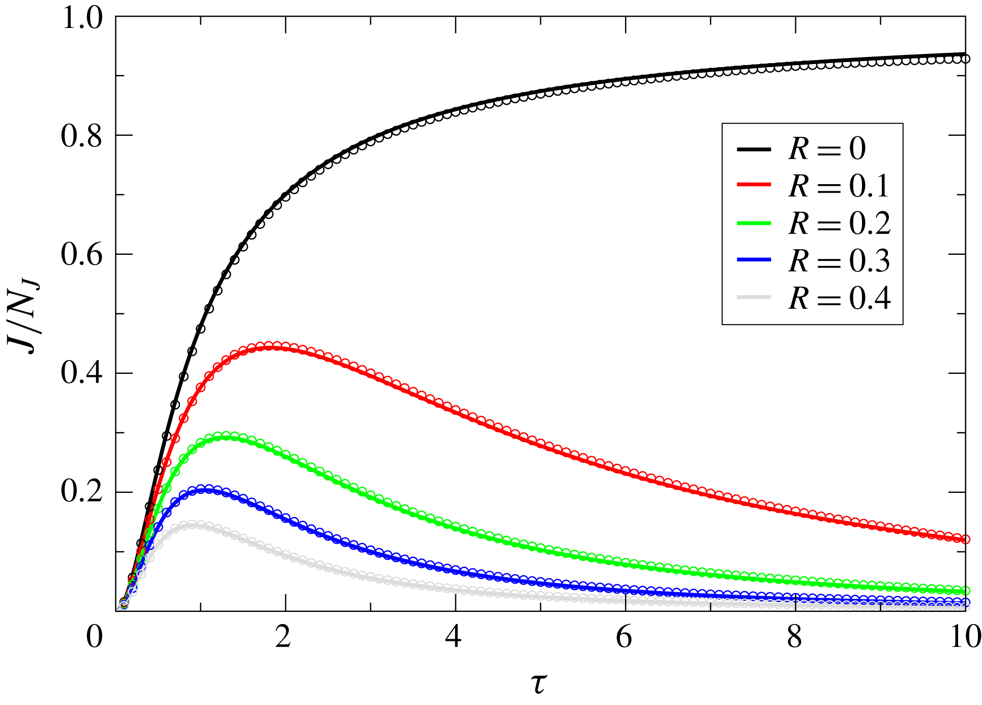
. Hence, this involves only a four-dimensional integral which becomes more amenable to numerical integration. The result of this will be shown in figure 1 which will be compared with Fedele’s result.
Evolution of normalized kurtosis versus time for different values of
 $R$
. Results using the expensive brute force method are shown as open circles.

Although (3.3) looks simpler, it still involves a singularity at
 $\unicode[STIX]{x0394}\unicode[STIX]{x1D714}=0$
. Now, Fedele et al. (Reference Fedele, Cherneva, Tayfun and Guedes Soares2010) suggest that this singularity can be removed by differentiating
 $J$
with respect to time, and afterwards the final result will be obtained by means of an integration in time. Indeed, with c.c. shorthand for complex conjugate, one finds
 $$\begin{eqnarray}\displaystyle \frac{\unicode[STIX]{x2202}J(R,\unicode[STIX]{x1D70F})}{\unicode[STIX]{x2202}\unicode[STIX]{x1D70F}}=-\text{i}\frac{3}{(2\unicode[STIX]{x03C0})^{2}}\int _{-\infty }^{\infty }\text{d}x_{1,2,3,4}\text{e}^{-(x_{1}^{2}+x_{2}^{2}-x_{1}x_{2})-(x_{3}^{2}+x_{4}^{2}-x_{3}x_{4})+\text{i}\unicode[STIX]{x0394}\unicode[STIX]{x1D714}\unicode[STIX]{x1D70F}}+\text{c.c.} & & \displaystyle\end{eqnarray}$$
These integrals have the form of Gaussian integrals, which can be integrated immediately as
 $$\begin{eqnarray}\displaystyle \int \text{d}\boldsymbol{x}\text{e}^{-\boldsymbol{x}^{\text{T}}\unicode[STIX]{x1D63C}\boldsymbol{x}}=\sqrt{\frac{\unicode[STIX]{x03C0}^{n}}{\text{Det}(\unicode[STIX]{x1D63C})}}, & & \displaystyle\end{eqnarray}$$
where
 $n$
is the size of the square matrix
 $\unicode[STIX]{x1D63C}$
. In the present case things are really straightforward, as in (3.5) there is no coupling between the pairs
 $(x_{1},x_{2})$
and
 $(x_{3},x_{4})$
so only the determinants of
 $2\times 2$
-matrices, called
 $\unicode[STIX]{x1D63D}$
and
 $\unicode[STIX]{x1D63E}$
, have to be obtained. Here the relevant matrix elements are
 $$\begin{eqnarray}\displaystyle & \displaystyle \unicode[STIX]{x1D609}_{11}=1,\unicode[STIX]{x1D609}_{12}=-(1+3\text{i}\unicode[STIX]{x1D70F})/2, & \displaystyle\end{eqnarray}$$
 $$\begin{eqnarray}\displaystyle & \displaystyle \unicode[STIX]{x1D609}_{21}=-(1+3\text{i}\unicode[STIX]{x1D70F})/2,\unicode[STIX]{x1D609}_{22}=1, & \displaystyle\end{eqnarray}$$
while
 $$\begin{eqnarray}\displaystyle & \displaystyle \unicode[STIX]{x1D60A}_{11}=1,\unicode[STIX]{x1D60A}_{12}=-(1-3\text{i}R\unicode[STIX]{x1D70F})/2, & \displaystyle\end{eqnarray}$$
 $$\begin{eqnarray}\displaystyle & \displaystyle \unicode[STIX]{x1D60A}_{21}=-(1-3\text{i}R\unicode[STIX]{x1D70F})/2,\unicode[STIX]{x1D60A}_{22}=1. & \displaystyle\end{eqnarray}$$
The corresponding determinants then become
 $\text{Det}(\unicode[STIX]{x1D63D})=(1-(1+3\text{i}\unicode[STIX]{x1D70F})^{2}/4)$
and
 $\text{Det}(\unicode[STIX]{x1D63E})=(1-(1-3\text{i}R\unicode[STIX]{x1D70F})^{2}/4)$
. Combining all this, the eventual result for the time derivative of
 $J$
is
 $$\begin{eqnarray}\displaystyle \frac{\unicode[STIX]{x2202}J(R,\unicode[STIX]{x1D70F})}{\unicode[STIX]{x2202}\unicode[STIX]{x1D70F}}=\frac{-\text{i}}{\{(1-2\text{i}\unicode[STIX]{x1D70F}+3\unicode[STIX]{x1D70F}^{2})(1+2\text{i}R\unicode[STIX]{x1D70F}+3R^{2}\unicode[STIX]{x1D70F}^{2})\}^{1/2}}+\text{c.c.}, & & \displaystyle\end{eqnarray}$$
so that
 $$\begin{eqnarray}\displaystyle J(R,\unicode[STIX]{x1D70F})=-\text{i}\int _{0}^{\unicode[STIX]{x1D70F}}\frac{\text{d}z}{\{(1-2\text{i}z+3z^{2})(1+2\text{i}Rz+3R^{2}z^{2})\}^{1/2}}+\text{c.c.} & & \displaystyle\end{eqnarray}$$
Here,
 $z$
is a complex variable,
 $z=x+\text{i}y$
, but for the moment it is assumed that the integration is along the real axis so that
 $z=x$
is real. For the purposes of numerical evaluation a bit more work is required since (3.11) is a complex integral and it involves branch points. The factor
 $1-2\text{i}z+3z^{2}$
gives two zeroes, namely at
 $z=\text{i}$
and at
 $z=-\text{i}/3$
while similarly the factor
 $1+2\text{i}Rz+3R^{2}z^{2}$
has zeroes at
 $Rz=\text{i}/3$
and at
 $Rz=-\text{i}$
. Thus, (3.11) becomes
 $$\begin{eqnarray}\displaystyle J(R,\unicode[STIX]{x1D70F})=-\frac{1}{3}\text{i}\int _{0}^{\unicode[STIX]{x1D70F}}\frac{\text{d}z}{(z-\text{i})^{1/2}(z+\frac{1}{3}\text{i})^{1/2}(Rz+\text{i})^{1/2}(Rz-\frac{1}{3}\text{i})^{1/2}}+\text{c.c.} & & \displaystyle\end{eqnarray}$$
It is now straightforward to do a numerical evaluation using for real
 $z$
 $$\begin{eqnarray}\displaystyle (z-\text{i}a)^{1/2}=\{z^{2}+a^{2}\}^{1/4}\text{e}^{\text{i}\unicode[STIX]{x1D703}/2},\quad \unicode[STIX]{x1D703}=\arctan (-a/z), & & \displaystyle\end{eqnarray}$$
so that
 $$\begin{eqnarray}\displaystyle J(R,\unicode[STIX]{x1D70F})=-\frac{2}{3}\int _{0}^{\unicode[STIX]{x1D70F}}\text{d}z\frac{\sin \frac{1}{2}(\unicode[STIX]{x1D703}_{1}+\unicode[STIX]{x1D703}_{2}+\unicode[STIX]{x1D703}_{3}+\unicode[STIX]{x1D703}_{4})}{\{(z^{2}+1)(z^{2}+\frac{1}{9})((Rz)^{2}+1)((Rz)^{2}+\frac{1}{9})\}^{1/4}}, & & \displaystyle\end{eqnarray}$$
with
 $\unicode[STIX]{x1D703}_{1}=-\arctan (1/z)$
,
 $\unicode[STIX]{x1D703}_{2}=\arctan (1/3z)$
,
 $\unicode[STIX]{x1D703}_{3}=\arctan (1/Rz)$
, and
 $\unicode[STIX]{x1D703}_{4}=-\arctan (1/3Rz)$
. By means of
 $\arctan (x)+\arctan (y)=\arctan (x+y/1-xy),xy<1$
, the angles can be ‘added’ so that
 $$\begin{eqnarray}\displaystyle \unicode[STIX]{x1D703}_{1}+\unicode[STIX]{x1D703}_{2}+\unicode[STIX]{x1D703}_{3}+\unicode[STIX]{x1D703}_{4}=\arctan \left\{\frac{2z(R-1)(1-3Rz^{2})}{9R^{2}z^{4}+z^{2}(3+3R^{2}+4R)+1}\right\}. & & \displaystyle\end{eqnarray}$$
It should be clear that the sine function in (3.14) plays an important role since the denominator in the integrand is positive. Thus from (3.15), we see immediately that for
 $R=1$
the sum of the angles always vanishes, hence there is no time evolution in that case. Also, the function
 $J(R,\unicode[STIX]{x1D70F})$
increases strictly for
 $0<\unicode[STIX]{x1D70F}<1/(3R)^{1/2}$
and decreases strictly for
 $\unicode[STIX]{x1D70F}>1/(3R)^{1/2}$
. Therefore,
 $J(R,\unicode[STIX]{x1D70F})$
has a unique maximum at
 $\unicode[STIX]{x1D70F}=1/(3R)^{1/2}$
. Likewise, for
 $R>1$
it can be shown that
 $J(R,\unicode[STIX]{x1D70F})$
has a unique minimum.
Equations (3.14) and (3.15) were implemented on the computer, and runs were made for different values of
 $R$
. It is remarked that Mori & Janssen (Reference Mori and Janssen2006) have studied the special case of the 1-D NLS equation, i.e.
 $R=0$
and it was found that for
 $BFI=1$
kurtosis evolves towards the constant
 $N_{J}=\unicode[STIX]{x03C0}/3\sqrt{3}$
. The evolution of
 $J=C_{4}/BFI^{2}$
, normalized with the factor
 $N_{J}$
, is shown in figure 1. This figure is essentially from Fedele (Reference Fedele2015) and we have reproduced it for the reader’s convenience. In perfect agreement with the results by Fedele (Reference Fedele2015), it shows that except for
 $R=0$
,
 $J$
has a maximum at finite time
 $=1/(3R)^{1/2}$
after which
 $J$
decays to zero for large times.
The present analytical result was validated by means of an expensive brute force method. The integral in (3.3) was discretized in each direction on a linear grid with a relative resolution of 0.1 and a range of
 $\pm 2.5$
. The results are given in figure 1 by means of the circles and a good agreement with (3.14)–(3.15) is noted. However, the term involving
 $\cos \unicode[STIX]{x0394}\unicode[STIX]{x1D714}\unicode[STIX]{x1D70F}/\unicode[STIX]{x0394}\unicode[STIX]{x1D714}$
is rapidly varying for large time
 $\unicode[STIX]{x1D70F}$
and therefore the brute force method fails, giving erratic results, beyond
 $\unicode[STIX]{x1D70F}\sim 15{-}20$
.
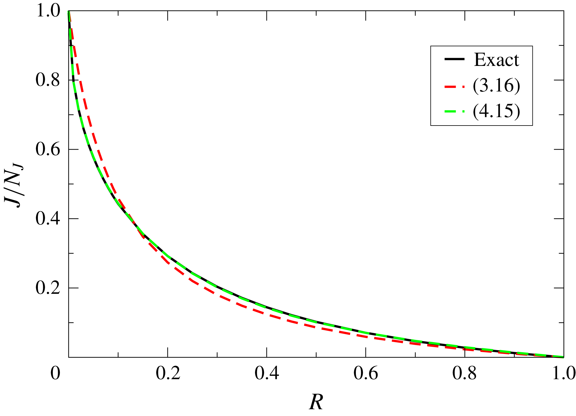
Finally, the dependence of the maximum value of
 $J$
over
 $\unicode[STIX]{x1D70F}>0$
, denoted by
 $J_{max}$
, on the relative width parameter
 $R$
was determined. This is shown in figure 2. A reasonable fit was found using
 $$\begin{eqnarray}\displaystyle \frac{J_{max}}{N_{J}}=\frac{R_{0}(1-R)}{R+R_{0}},\quad N_{J}=\frac{\unicode[STIX]{x03C0}}{3\sqrt{3}}, & & \displaystyle\end{eqnarray}$$
with
 $R_{0}=7.44\sqrt{3}/4\unicode[STIX]{x03C0}^{3}$
, which was found by trial and error. Observe that the right-hand side of (3.16) equals 1 at
 $R=0$
, while it vanishes for
 $R=1$
. This fit agrees with what is given in Fedele (Reference Fedele2015), except that there is a misprint in the definition of
 $R_{0}$
which seems to miss a factor
 $(2\unicode[STIX]{x03C0})^{2}$
. In the sequel, we shall find several analytical results for
 $J_{max}$
that are used to develop the compromise fit, also shown in figure 2.


4 Some analytical results on
 $J(R,\unicode[STIX]{x1D70F})$

4.1 Proof that for
$R>0$
the integral
$J$
vanishes for
$\unicode[STIX]{x1D70F}\rightarrow \infty$


It is important to prove that for large
 $\unicode[STIX]{x1D70F}$
the integral
 $J$
vanishes,
 $J(R,\unicode[STIX]{x1D70F}=\infty )=0$
. At least two proofs of this are known to us. The argument used in Fedele (Reference Fedele2015), p. 28, to prove this gives that
 $\lim _{\unicode[STIX]{x1D70F}\infty }J(R,\unicode[STIX]{x1D70F})$
indeed exists, but it is not obvious that this limit indeed equals 0; also see the discussion on this matter below.
The first proof starts from (3.12) which is regarded for now as an integral along the real axis. We have seen that the integral
 $J$
has a maximum at
 $\unicode[STIX]{x1D70F}=1/\sqrt{3R}$
and we regard this as a special point along the integration path. Therefore, we write
 $$\begin{eqnarray}\displaystyle J(R,\unicode[STIX]{x1D70F}=\infty )={\textstyle \frac{2}{3}}\text{Im}[I_{1}+I_{2}], & & \displaystyle\end{eqnarray}$$
where
 $$\begin{eqnarray}\displaystyle I_{1}=\int _{0}^{1/\sqrt{3R}}\frac{\text{d}z}{N(z)},\quad I_{2}=\int _{1/\sqrt{3R}}^{\infty }\frac{\text{d}z}{N(z)}, & & \displaystyle\end{eqnarray}$$
with
 $N(z)=(z-\text{i})^{1/2}(z+(1/3)\text{i})^{1/2}(Rz+\text{i})^{1/2}(Rz-(1/3)\text{i})^{1/2}$
. The next step is to introduce a transformation of variables in the second integral in such a way that the integration range becomes identical to the integration range of the first integral. The transformation
 $$\begin{eqnarray}\displaystyle z=\frac{1}{3Rw}, & & \displaystyle\end{eqnarray}$$
with Jacobian
 $=-1/3Rw^{2}$
, hence
 $\text{d}z=-\text{d}w/3Rw^{2}$
, indeed changes the integration range from
 $[1/\sqrt{3R},\infty ]$
to
 $[0,1/\sqrt{3R}]$
. Now, the important point to note is that under this transformation the function
 $N(z)$
is invariant in the sense that, apart from the Jacobian of the transformation, it equals the complex conjugate of
 $N(w)$
, i.e.
 $$\begin{eqnarray}\displaystyle N(z)=\frac{1}{3Rw^{2}}N^{\ast }(w). & & \displaystyle\end{eqnarray}$$
Therefore, using the transformation (4.3) in the integral
 $I_{2}$
, we find that
 $I_{2}=I_{1}^{\ast }$
so that
 $$\begin{eqnarray}\displaystyle J(R,\unicode[STIX]{x1D70F}=\infty )={\textstyle \frac{2}{3}}\text{Im}[I_{1}+I_{1}^{\ast }]=0, & & \displaystyle\end{eqnarray}$$
i.e. the integral
 $J$
vanishes for large times. The restriction to this result is that it only holds for finite
 $R$
since for vanishing
 $R$
there is no maximum of
 $J$
for finite time.
It is emphasized that the vanishing of the integral
 $J$
, and hence kurtosis for large time, is not a property for arbitrary spectral shape. We think that this property is closely connected to the ‘invariance’ property (4.4) of the denominator
 $N(z)$
which in the end is determined by our choice of a Gaussian spectrum (2.25). Numerical computations for spectra that are not symmetrical with respect the peak frequency do give a non-zero value of kurtosis for large time.
The second proof is rather involved, but in the end it utilizes the same invariance property for
 $N(z)$
to show the vanishing of
 $J$
. This proof regards the integral in (3.12) as an integral in the complex domain, and one applies the theorem that if there are no singularities inside the domain of a closed contour then the resulting integral vanishes. The contour was chosen to be (a)
 $0<x<\infty$
, (b) the circle with large radius
 $\unicode[STIX]{x1D70C}$
and phase
 $\unicode[STIX]{x1D703}$
with
 $0<\unicode[STIX]{x1D703}<\unicode[STIX]{x03C0}/2$
, and then back to the origin from
 $y=+\text{i}\infty$
to
 $y=0$
. Now, because of the branch points in (3.12), branch cuts need to be introduced, and basically this is done along the imaginary axis from the largest positive branch point to the smallest negative branch point. The phases of all relevant functions are then well defined. In addition, for
 $R>0$
one can show that the integral along the circle with large radius vanishes as
 $\unicode[STIX]{x1D70C}\rightarrow \infty$
, and therefore the integral along the real axis can be expressed in terms of the integral along the imaginary axis. The advantage is, namely, that the integral along the imaginary axis is much simpler. In fact, one finds for
 $R<1/3$
 $$\begin{eqnarray}\displaystyle J(R,\infty )=\frac{1}{3}\left\{\int _{0}^{1}\frac{\text{d}y}{N}-\int _{1/3R}^{\infty }\frac{\text{d}y}{N}\right\}, & & \displaystyle\end{eqnarray}$$
where
 $N=\{|y-1||y+1/3||Ry+1||Ry-1/3|\}^{1/2}$
. For
 $R>1/3$
a similar result is found. In the final step it can be shown that the two integrals cancel each other, therefore
 $J(\unicode[STIX]{x1D70F}\rightarrow \infty )$
vanishes. The easiest way to show this is by means of a transformation of the integration variable in the second integral, i.e.
 $y=1/3Rx$
, which is identical to the transformation (4.3)! For completeness details of this calculation are given in appendix A.
The contour integration approach, as employed in the second proof, can be used to establish further analytic results. This is done in all detail in appendix C, where the behaviour of
 $\max _{\unicode[STIX]{x1D70F}}J(R,\unicode[STIX]{x1D70F})$
near
 $R=0$
is obtained. The proof technique in appendix C can, furthermore, be used to obtain an expression of
 $J(R,1/\sqrt{3R})$
in terms of the incomplete elliptic integral of the first kind.


4.2 Decay of
$J(R,\unicode[STIX]{x1D70F})$
as
$\unicode[STIX]{x1D70F}\rightarrow \infty$


Having established that the integral
 $J$
of (3.12) vanishes for large dimensionless time
 $\unicode[STIX]{x1D70F}$
, we now study how
 $J$
approaches this limit. Starting from (3.12) we have
 $$\begin{eqnarray}\displaystyle J(R,\unicode[STIX]{x1D70F})=\frac{2}{3}\text{Im}\int _{0}^{\unicode[STIX]{x1D70F}}\frac{\text{d}z}{N(z)}=-\frac{2}{3}\text{Im}\int _{\unicode[STIX]{x1D70F}}^{\infty }\frac{\text{d}z}{N(z)}, & & \displaystyle\end{eqnarray}$$
where again
 $N(z)=(z-\text{i})^{1/2}(z+(1/3)\text{i})^{1/2}(Rz+\text{i})^{1/2}(Rz-(1/3)\text{i})^{1/2}$
. The large time behaviour of
 $J$
is now found by expanding the integrand of the second integral of (4.7) into powers of
 $1/z$
and integrating the expansion. The details of this calculation are given in appendix B, and the final result is
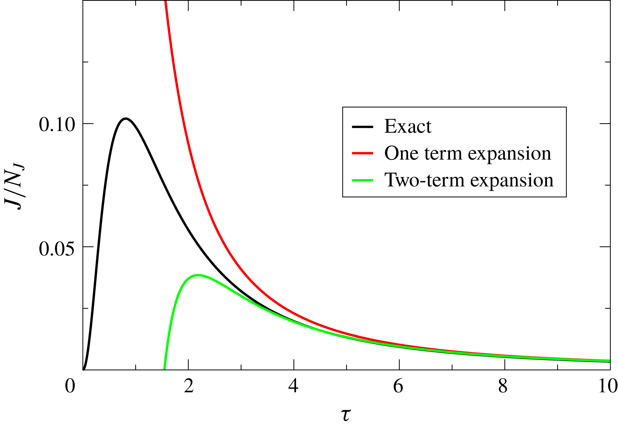
 $$\begin{eqnarray}\displaystyle J(R,\unicode[STIX]{x1D70F})=\frac{1}{R}\left(\frac{1}{R}-1\right)\left[\frac{1}{9\unicode[STIX]{x1D70F}^{2}}-\left(\frac{7}{R^{2}}+\frac{4}{R}+7\right)\frac{1}{162\unicode[STIX]{x1D70F}^{4}}+\cdots \!\right], & & \displaystyle\end{eqnarray}$$
an expansion which is valid for
 $\unicode[STIX]{x1D70F}>1/R$
, as is verified in figure 3, which compares the exact result for
 $R=0.5$
with the above asymptotic expansion. The first term in (4.8) agrees with what can be obtained from Fedele (Reference Fedele2015), (3.5). The second-order term has a surprisingly large impact for moderate values of dimensionless time
 $\unicode[STIX]{x1D70F}$
.


4.3 Behaviour of
$\max _{\unicode[STIX]{x1D70F}}J(R,\unicode[STIX]{x1D70F})$
as
$R\downarrow 0$


It is important to have an estimate of the severity of the sea state during extreme events. Such an indicator may be provided by the maximum of the excess kurtosis as a function of time. It is therefore of interest to get an estimate of the maximum of the integral
 $J$
, which occurs at time
 $\unicode[STIX]{x1D70F}=1/\sqrt{3R}$
. For
 $0<R<1$
we have
 $$\begin{eqnarray}\displaystyle \max _{\unicode[STIX]{x1D70F}\geqslant 0}J(R,\unicode[STIX]{x1D70F})=J\left(R,\frac{1}{\sqrt{3R}}\right), & & \displaystyle\end{eqnarray}$$
where
 $J(R,\unicode[STIX]{x1D70F})$
is given by the last expression in (4.7). The detailed analysis is given in appendix C. Taylor expansion around
 $R=0$
then gives the eventual result
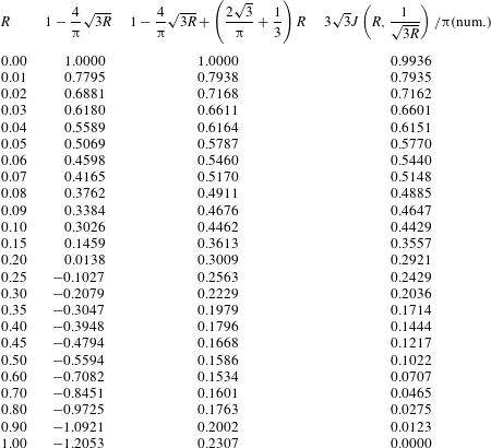
 $$\begin{eqnarray}\displaystyle J\left(R,\frac{1}{\sqrt{3R}}\right)=\frac{\unicode[STIX]{x03C0}}{3\sqrt{3}}\left(1-\frac{4}{\unicode[STIX]{x03C0}}\sqrt{3R}+\left(\frac{2\sqrt{3}}{\unicode[STIX]{x03C0}}+\frac{1}{3}\right)R+O(R^{3/2})\right). & & \displaystyle\end{eqnarray}$$
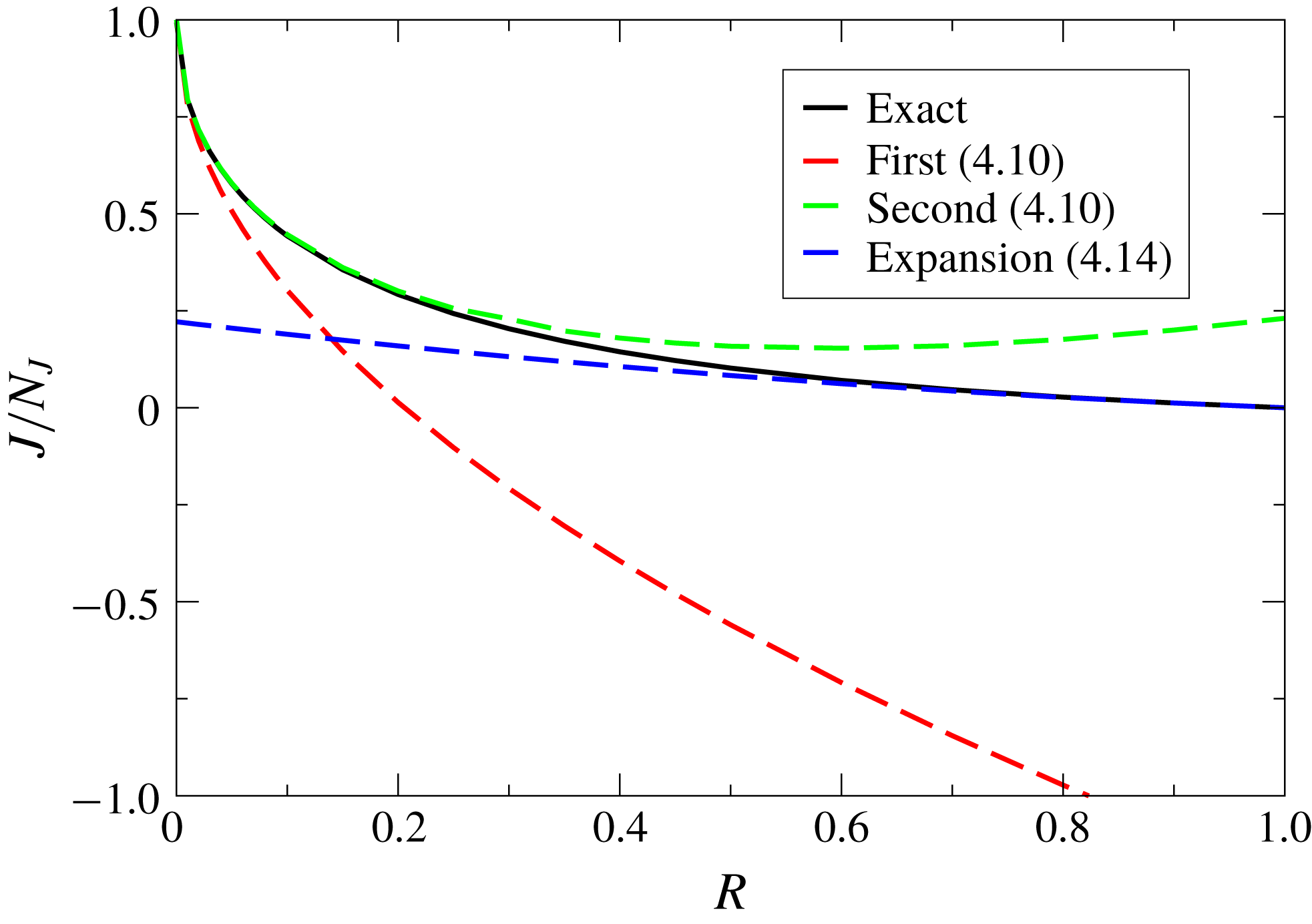
The first term of this Taylor expansion agrees with what can be found from Fedele (Reference Fedele2015), (4.3), (4.5). In order to assess the accuracy of the approximation (4.10), we compare in figure 4 the values of the first-order approximation and the second-order approximation with the numerically computed value of
 $J(R,1/\sqrt{3R})$
, normalized with
 $\unicode[STIX]{x03C0}/3\sqrt{3}$
. Although the first-order approximation deviates quite quickly from the ‘exact’ result, it is rewarding to see how much the second-order term improves the agreement with ‘exact’ up to values of
 $R=0.4$
. This is surprising as the expansion in (4.10) has a radius of convergence of only
 $1/3$
.
Here it is mentioned that once more, we use complex analysis and Cauchy’s theorem to simplify the integral. The contour integration approach can be used to classify the integral
 $J(R,1/\sqrt{3R})$
in terms of the incomplete elliptic integral of the first kind that is available in many mathematical packages. This result is also instrumental for checking numerical work. It can then be shown that
 $$\begin{eqnarray}\displaystyle J\left(R,\frac{1}{\sqrt{3R}}\right)=\left\{\begin{array}{@{}l@{}}\displaystyle \frac{k}{\sqrt{R}}(F(x_{1},k)-F(x_{2},k)),\quad 0\leqslant R<\frac{1}{3},\\ \displaystyle \frac{1}{\sqrt{R}}(F(x_{1}^{-1},k^{-1})-F(x_{2}^{-1},k^{-1})),\quad \frac{1}{3}<R\leqslant 1,\end{array}\right. & & \displaystyle\end{eqnarray}$$
where
 $$\begin{eqnarray}\displaystyle k=\frac{4\sqrt{3R}}{3(1+R)},\quad x_{1}=\frac{1}{2}\sqrt{3(1+R)},\quad x_{2}=\frac{(3+\sqrt{3R})\sqrt{R+\frac{1}{3}}-(1-\sqrt{3R})\sqrt{R+3}}{\sqrt{32R}}, & & \displaystyle \nonumber\\ \displaystyle & & \displaystyle\end{eqnarray}$$
and, for
 $0\leqslant x<1$
,
 $0\leqslant k\leqslant 1$
,
 $$\begin{eqnarray}\displaystyle F(x,k)=\int _{0}^{x}\frac{\text{d}t}{\sqrt{(1-t^{2})(1-k^{2}t^{2})}}, & & \displaystyle\end{eqnarray}$$
the incomplete elliptic integral of the first kind. The proof of this result is quite involved, and we omit it. Using the Keisan Online Calculator we found perfect agreement with the numerical results for
 $J(R,1/\sqrt{3R})$
in table 1 of appendix C.
4.4 Behaviour of
$\max _{\unicode[STIX]{x1D70F}}J(R,\unicode[STIX]{x1D70F})$
as
$R\rightarrow 1$


In appendix D the behaviour of
 $\max _{\unicode[STIX]{x1D70F}}J(R,\unicode[STIX]{x1D70F})=J(R,1/\sqrt{3R})$
is obtained as
 $R\rightarrow 1$
. The result is
 $$\begin{eqnarray}\displaystyle J(R,1/\sqrt{3R})=({\textstyle \frac{1}{2}}-{\textstyle \frac{1}{4}}\sqrt{3})\{(1-R)+(1-R)^{2}\}+O((1-R)^{3}). & & \displaystyle\end{eqnarray}$$
This result is derived in a straightforward manner from the expression (3.12) for
 $J(R,\unicode[STIX]{x1D70F}=1/\sqrt{3R})$
by differentiation. Observe that the coefficients of
 $(1-R)$
and
 $(1-R)^{2}$
in (4.14) are identical. The expansion (4.14), without the term
 $O((1-R)^{3})$
, is shown in figure 4, and shows good agreement with the numerical result in the range
 $0.6<R<1$
.
4.5 Approximating
$\max _{\unicode[STIX]{x1D70F}}J(R,\unicode[STIX]{x1D70F})$
on the range
$0<R<1$


We wonder whether it would be possible to use the approximation (4.10) and (4.14) in a compromise fit so as to get a reasonable approximation over the whole range
 $0<R<1$
. Due to the highly different nature, as a function of
 $R$
, of
 $J(R,1/\sqrt{3R})$
near
 $R=0$
and
 $R=1$
, a simple convex combination of (4.10) and (4.14) fails to give such an approximation. Instead we propose the approximation
 $$\begin{eqnarray}\displaystyle J\left(R,\frac{1}{\sqrt{3R}}\right)\approx \frac{\unicode[STIX]{x03C0}}{3\sqrt{3}}(1-\unicode[STIX]{x1D6FC}\sqrt{R}+\unicode[STIX]{x1D6FD}R+\unicode[STIX]{x1D6FF}R^{2}),\quad 0<R<1, & & \displaystyle\end{eqnarray}$$
where
 $\unicode[STIX]{x1D6FC}=4\sqrt{3}/\unicode[STIX]{x03C0}$
and
 $\unicode[STIX]{x1D6FD}=(1/3+2\sqrt{3}/\unicode[STIX]{x03C0})$
, see (4.10), and
 $\unicode[STIX]{x1D6FF}$
to be chosen such that both sides of (4.15) agree at
 $R=1$
. This gives the condition
 $1-\unicode[STIX]{x1D6FC}+\unicode[STIX]{x1D6FD}+\unicode[STIX]{x1D6FF}=0$
from which
 $\unicode[STIX]{x1D6FF}=2\sqrt{3}/\unicode[STIX]{x03C0}-4/3=-0.2307$
. The compromise fit (4.15) is compared with the simple fit (3.16) and with the exact result obtained numerically in figure 2. The compromise fit achieves a maximum absolute error in (4.15) of the order
 $10^{-3}$
, and thus outperforms fit (3.16) by far. Furthermore, the values of the derivatives of both sides in (4.15) at
 $R=1$
are
 $-0.0670$
and
 $-0.0774$
, respectively.
We also tried a compromise fit of the form
 $$\begin{eqnarray}\displaystyle J\left(R,\frac{1}{\sqrt{3R}}\right)\approx \frac{\unicode[STIX]{x03C0}}{3\sqrt{3}}(1-\unicode[STIX]{x1D6FC}\sqrt{R}+\unicode[STIX]{x1D6FD}R++\unicode[STIX]{x1D6FE}R^{3/2}+\unicode[STIX]{x1D6FF}R^{2}),\quad 0<R<1, & & \displaystyle\end{eqnarray}$$
with
 $\unicode[STIX]{x1D6FC}$
and
 $\unicode[STIX]{x1D6FD}$
as in (4.15) and
 $\unicode[STIX]{x1D6FE}$
and
 $\unicode[STIX]{x1D6FF}$
such that (i) both sides of (4.16) and their derivatives agree at
 $R=1$
, or, (ii) both sides of (4.16) agree at
 $R=1$
and
 $R=1/3$
. It was found that these fits do not improve the fit (4.15), with fit (i) systematically too small and fit (ii) systematically too large on a large part of the range
 $0<R<1$
. The average of the fits (i) and (ii) performs about as good as fit (4.15), with parameter values
 $\unicode[STIX]{x1D6FE}=-0.0070$
,
 $\unicode[STIX]{x1D6FF}=-0.2237$
that are remarkably close to the parameter values
 $\unicode[STIX]{x1D6FE}=0.0000,\unicode[STIX]{x1D6FF}=-0.2307$
pertaining to fit (4.15).
5 Conclusions
In this paper we emphasize that extreme events such as freak waves are a transient phenomenon as soon as the wave propagation is not purely unidirectional. This follows immediately from figure 1 which shows the evolution of excess kurtosis versus time. A general evolution equation for excess kurtosis was obtained by Janssen (Reference Janssen2003) and the figure 1 shows the special case of a weakly nonlinear, narrow-band wave train, the dynamics of which is governed by the NLS equation. The wave spectrum is chosen to be a Gaussian which is symmetric with respect to the peak frequency. For this special case it is straightforward to find the conditions for which extreme events are generated. Clearly, for surface gravity waves in one dimension wave energy is focused, even for large times. As soon as two-dimensional effects are introduced the formation of extreme events shows transient behaviour. A maximum in kurtosis will be reached provided the wave spectra are sufficiently narrow in direction, i.e.
 $R<1$
. For Gaussian spectra the extremum in excess kurtosis is reached for dimensionless time
 $\unicode[STIX]{x1D70F}=1/\sqrt{3R}$
, after which kurtosis will decaytowards zero for large times. From operational ECMWF wave spectra one may gain insight into the order of magnitude of the dimensionless directional width
 $R$
. Values of
 $R$
then range from 0.25 to 4 indicating that in the field there is a finite number of cases where
 $R<1$
, i.e. there is nonlinear focusing of wave energy.
It is of interest to give an estimate of time scales in terms of commonly reported values of parameters involved. However, it should be realized that the NLS equation is a poor approximation to the case of ocean waves because their spectra are too broad for the NLS equation to be valid. Also, Gaussian spectra are not the norm in nature. We therefore use as an example laboratory experiments (Onorato et al.
Reference Onorato, Waseda, Toffoli, Cavaleri, Gramstad, Janssen, Kinoshita, Monbaliu, Mori, Osborne, Serio, Stansberg, Tamura and Trulsen2009) where spectra are generated by a programmable wave maker. With a relative frequency width
 $\unicode[STIX]{x1D6FF}_{\unicode[STIX]{x1D714}}$
of 0.1 and a
 $5^{\circ }$
angular width, hence
 $\unicode[STIX]{x1D6FF}_{\unicode[STIX]{x1D703}}=0.087$
, one then finds that
 $R=0.38$
so that
 $\unicode[STIX]{x1D70F}_{max}=1/\sqrt{3R}\approx 1$
. In real terms this means that
 $t_{max}=1/\unicode[STIX]{x1D6FF}_{\unicode[STIX]{x1D714}}^{2}\unicode[STIX]{x1D714}_{0}=T_{0}/2\unicode[STIX]{x03C0}\unicode[STIX]{x1D6FF}_{\unicode[STIX]{x1D714}}^{2}\approx 16T_{0}$
, where
 $T_{0}$
is the peak period. From figure 1 it is seen that the decay phase is two to three times longer than the growth phase of the extreme event so that according to this example an extreme event lasts about 50 wave periods. Translating this to the field (but noting the caveats above), and taking as a typical period of the waves 10 s, then such an event will last approximately 10 min, which is much shorter than the typical duration of a storm, which lasts 6 h or more. Although qualitatively correct, the NLS equation is a poor approximation to the case of ocean waves. Nevertheless, starting from computations of the complete expressions for skewness and kurtosis using realistic ocean wave spectra it is possible, guided by the narrow-band expressions for the wave statistics, to obtain parametrizations for skewness and kurtosis. This is still work in progress which is reported in Janssen (Reference Janssen2017). Based on these parametrizations one gets time scales for extreme events which are somewhat longer than obtained from the NLS equation, namely 30 min rather than 10 min. However, this is still shorter than the typical duration of a storm. In addition, using operational ECMWF wave spectra, one may get insight into the order of magnitude of the kurtosis and it is found for some special cases, such as the Draupner event or the Andrea storm, that exceedance probabilities for maximum wave height increase by a factor of two to three.
In this paper we have given some intriguing analytic properties of the exact solution of the simplified problem, resulting in a new, accurate parametrization of the maximum of excess kurtosis as function of the Benjamin–Feir index and the dimensionless directional width
 $R$
. This parametrization will be shortly implemented in ECMWF’s freak wave warning system.
Acknowledgements
The authors much appreciate the comments of the reviewers which improved the present paper considerably.
Appendix A. Alternative proof that
$J(R,\unicode[STIX]{x1D70F}=\infty )=0$
(
$0<R<1$
)


Consider the integral
 $$\begin{eqnarray}\displaystyle J(R,\unicode[STIX]{x1D70F})=-\frac{\text{i}}{3}\int _{\unicode[STIX]{x1D6E4}}\frac{\text{d}z}{\displaystyle (z-\text{i})^{1/2}\left(z+\frac{\text{i}}{3}\right)^{1/2}(Rz+\text{i})^{1/2}\left(Rz-\frac{\text{i}}{3}\right)^{1/2}}+\text{c.c.}, & & \displaystyle\end{eqnarray}$$
with complex
 $z=x+\text{i}y$
and
 $\unicode[STIX]{x1D6E4}$
a conveniently defined contour in the complex
 $z$
plane. Thus far the integration contour was taken along the real axis, but as seen from (3.14) the resulting integral is rather complicated, involving a sine function with a complicated argument so that it is not so straightforward to take the limit for large
 $\unicode[STIX]{x1D70F}$
. Here, we use Cauchy’s residue theorem together with Jordan’s lemma to explore alternative ways of evaluating the integral
 $J$
.
From the form of the integrand it is evident that there are branch points in this problem at
 $z=\text{i},z=-\text{i}/3,z=-\text{i}/R,$
and
 $z=\text{i}/3R$
, and branch cuts need to be introduced because when one loops around such a branch point jumps in the phase occur. Here, a branch cut is introduced from
 $-\text{i}/R$
to
 $\text{i}$
along the imaginary axis. For real
 $a$
one may write
 $$\begin{eqnarray}\displaystyle (z-\text{i}a)^{1/2}=\unicode[STIX]{x1D70C}^{1/2}\text{e}^{\text{i}\unicode[STIX]{x1D703}/2}, & & \displaystyle\end{eqnarray}$$
with
 $\unicode[STIX]{x1D70C}=\sqrt{x^{2}+(y-a)^{2}}$
, and
 $\unicode[STIX]{x1D703}=\arctan [(y-a)/x]$
. In general, the integral
 $J$
may therefore be written as
 $$\begin{eqnarray}\displaystyle J(R,\unicode[STIX]{x1D70F})=-\frac{\text{i}}{3R}\int _{\unicode[STIX]{x1D6E4}}\text{d}z\frac{\text{e}^{-\text{i}(\unicode[STIX]{x1D703}_{1}+\unicode[STIX]{x1D703}_{2}+\unicode[STIX]{x1D703}_{3}+\unicode[STIX]{x1D703}_{4})/2}}{(\unicode[STIX]{x1D70C}_{1}\unicode[STIX]{x1D70C}_{2}\unicode[STIX]{x1D70C}_{3}\unicode[STIX]{x1D70C}_{4})^{1/2}}+\text{c.c.}, & & \displaystyle\end{eqnarray}$$
where the index ‘1’ corresponds to
 $(0,1)$
in the complex domain, ‘2’ to
 $(0,1/3)$
, ‘3’ to
 $(0,-1/R)$
and ‘4’ to
 $(0,1/3R)$
.
Let us now apply (A 3) for a particular contour
 $\unicode[STIX]{x1D6E4}$
given by three segments:
 $\unicode[STIX]{x1D6E4}_{R}$
,
 $x=+0\rightarrow \unicode[STIX]{x1D70C}$
,
 $y=0$
;
 $\unicode[STIX]{x1D6E4}_{C}$
, circle with radius
 $\unicode[STIX]{x1D70C}$
and
 $\unicode[STIX]{x1D703}$
from
 $0\rightarrow \unicode[STIX]{x03C0}/2$
;
 $\unicode[STIX]{x1D6E4}_{I}$
along the imaginary axis from
 $z=\text{i}\unicode[STIX]{x1D70C}$
to
 $z=0$
to the right of the branch cut.
Since there are no singularities inside the domain bordered by
 $\unicode[STIX]{x1D6E4}$
we have
 $$\begin{eqnarray}\displaystyle \int _{\unicode[STIX]{x1D6E4}_{R}}+\int _{\unicode[STIX]{x1D6E4}_{C}}+\int _{\unicode[STIX]{x1D6E4}_{I}}=0. & & \displaystyle\end{eqnarray}$$
We have already derived the integral along the real axis in (3.14), but, as already noted, from this expression it is hard to determine the large time behaviour of
 $J$
. Let us therefore consider the integral along the segments
 $\unicode[STIX]{x1D6E4}_{C}$
and
 $\unicode[STIX]{x1D6E4}_{I}$
.
A.1 The contour
$\unicode[STIX]{x1D6E4}_{C}$

Let us consider now the contour
 $\unicode[STIX]{x1D6E4}_{C}$
for large radius
 $\unicode[STIX]{x1D70C}$
. Then
 $$\begin{eqnarray}\displaystyle \unicode[STIX]{x1D70C}_{1}\unicode[STIX]{x1D70C}_{2}\unicode[STIX]{x1D70C}_{3}\unicode[STIX]{x1D70C}_{4}\rightarrow \unicode[STIX]{x1D70C}^{4}, & & \displaystyle\end{eqnarray}$$
so that
 $$\begin{eqnarray}\displaystyle J_{C}\rightarrow \frac{1}{3R\unicode[STIX]{x1D70C}}\int _{0}^{\unicode[STIX]{x03C0}/2}\text{d}\unicode[STIX]{x1D703}\text{e}^{-2\text{i}\unicode[STIX]{x1D703}}+\text{c.c.}, & & \displaystyle\end{eqnarray}$$
hence if
 $R\neq 0$
then
 $$\begin{eqnarray}\displaystyle \lim _{\unicode[STIX]{x1D70C}\rightarrow \infty }J_{C}\rightarrow 0. & & \displaystyle\end{eqnarray}$$
A.2 The contour
$\unicode[STIX]{x1D6E4}_{I}$

Consider now the contour
 $\unicode[STIX]{x1D6E4}_{I}$
. Two cases need to be distinguished, namely
 $R<1/3$
and
 $R>1/3$
. Consider first
 $R<1/3$
. Then for
 $y>1/3R$
we have (with
 $x\rightarrow +0$
):
 $$\begin{eqnarray}\displaystyle \unicode[STIX]{x1D703}_{1}=\unicode[STIX]{x03C0}/2,\quad \unicode[STIX]{x1D703}_{2}=\unicode[STIX]{x03C0}/2,\quad \unicode[STIX]{x1D703}_{3}=\unicode[STIX]{x03C0}/2,\quad \unicode[STIX]{x1D703}_{4}=\unicode[STIX]{x03C0}/2, & & \displaystyle\end{eqnarray}$$
while for
 $1<y<1/3R$
we have
 $$\begin{eqnarray}\displaystyle \unicode[STIX]{x1D703}_{1}=\unicode[STIX]{x03C0}/2,\quad \unicode[STIX]{x1D703}_{2}=\unicode[STIX]{x03C0}/2,\quad \unicode[STIX]{x1D703}_{3}=\unicode[STIX]{x03C0}/2,\quad \unicode[STIX]{x1D703}_{4}=-\unicode[STIX]{x03C0}/2, & & \displaystyle\end{eqnarray}$$
while, finally, for
 $0<y<1$
we have
 $$\begin{eqnarray}\displaystyle \unicode[STIX]{x1D703}_{1}=-\unicode[STIX]{x03C0}/2,\quad \unicode[STIX]{x1D703}_{2}=\unicode[STIX]{x03C0}/2,\quad \unicode[STIX]{x1D703}_{3}=\unicode[STIX]{x03C0}/2,\quad \unicode[STIX]{x1D703}_{4}=-\unicode[STIX]{x03C0}/2. & & \displaystyle\end{eqnarray}$$
In other words, every time one passes a branch point the phase of the corresponding factor in the integrand jumps by
 $-\unicode[STIX]{x03C0}$
. As a consequence
 $J_{I}$
becomes
 $$\begin{eqnarray}\displaystyle J_{I}=\frac{1}{3}\left[\int _{\infty }^{1/3R}\text{d}y\frac{\text{e}^{-\unicode[STIX]{x03C0}\text{i}}}{N}+\int _{1/3R}^{1}\text{d}y\frac{\text{e}^{-\unicode[STIX]{x03C0}\text{i}/2}}{N}+\int _{1}^{0}\text{d}y\frac{\text{e}^{0}}{N}\right]+\text{c.c.}, & & \displaystyle\end{eqnarray}$$
with
 $N=\{|y-1||y+1/3||Ry+1||Ry-1/3|\}^{1/2}$
.
Now apply (A 4) then, as the integral over the quarter circle vanishes, we have
 $$\begin{eqnarray}\displaystyle \int _{\unicode[STIX]{x1D6E4}_{R}}=-\int _{\unicode[STIX]{x1D6E4}_{I}}, & & \displaystyle\end{eqnarray}$$
and the kurtosis becomes
 $$\begin{eqnarray}\displaystyle J=-\int _{\unicode[STIX]{x1D6E4}_{I}}+\,\text{c.c.}, & & \displaystyle\end{eqnarray}$$
or, for
 $R<1/3$
,
 $$\begin{eqnarray}\displaystyle J=\frac{2}{3}\left[\int _{0}^{1}\frac{\text{d}y}{N}-\int _{1/3R}^{\infty }\frac{\text{d}y}{N}\right], & & \displaystyle\end{eqnarray}$$
while in a similar fashion one finds for
 $R>1/3$
 $$\begin{eqnarray}\displaystyle J=\frac{2}{3}\left[\int _{0}^{1/3R}\frac{\text{d}y}{N}-\int _{1}^{\infty }\frac{\text{d}y}{N}\right], & & \displaystyle\end{eqnarray}$$
In the final step, it needs to be shown that the two integrals cancel each other, therefore that
 $J(\unicode[STIX]{x1D70F}\rightarrow \infty )$
vanishes. In order to show this, consider the case
 $R<1/3$
and define
 $$\begin{eqnarray}\displaystyle {\mathcal{A}}=\int _{1/3R}^{\infty }\frac{\text{d}y}{N},\quad {\mathcal{B}}=\int _{0}^{1}\frac{\text{d}y}{N}. & & \displaystyle\end{eqnarray}$$
Introduce as integration variable
 $x=1/3Ry$
then
 $$\begin{eqnarray}\displaystyle {\mathcal{A}}=\frac{1}{3R}\int _{0}^{1}\,\text{d}x\left\{\left|\frac{1}{3R}-x\right|\left|\frac{1}{3R}+\frac{x}{3}\right|\left|\frac{1}{3}+x\right|\left|\frac{1}{3}-\frac{x}{3}\right|\right\}^{-1/2}, & & \displaystyle\end{eqnarray}$$
and this equals
 ${\mathcal{B}}$
as is easily found after some algebra. Therefore, it has been shown that
 $J$
vanishes for
 $\unicode[STIX]{x1D70F}\rightarrow \infty$
for
 $R\neq 0$
.
A.3 The case
$R=0$

The case
 $R=0$
is an exception. First of all, the phase is then zero and the integral along the real part can be evaluated immediately. Secondly, it turns out now that the integral along the quarter circle does not vanish, but amounts to a value of
 $\unicode[STIX]{x03C0}\sqrt{3}/3$
, while also the integral along the imaginary axis gives a contribution in such a way that the sum
 $-\unicode[STIX]{x1D6E4}_{C}-\unicode[STIX]{x1D6E4}_{I}$
equals
 $\unicode[STIX]{x03C0}/3\sqrt{3}$
, which is the usual result for kurtosis in the one-dimensional case for large time.
Appendix B. Decay of
$J(R,\unicode[STIX]{x1D70F})$
as
$\unicode[STIX]{x1D70F}\rightarrow \infty$


We have by the main result in § 3 and
 $J(R,\infty )=0$
that for
 $0<R<1$
 $$\begin{eqnarray}\displaystyle J(R,\unicode[STIX]{x1D70F}) & = & \displaystyle \frac{2}{3}\text{Im}\left[\int _{0}^{\unicode[STIX]{x1D70F}}\frac{\text{d}z}{(z-\text{i})^{1/2}(z+\frac{1}{3}\text{i})^{1/2}(Rz+\text{i})^{1/2}(Rz-\frac{1}{3}\text{i})^{1/2}}\right]\nonumber\\ \displaystyle & = & \displaystyle -\frac{2}{3}\text{Im}\left[\int _{\unicode[STIX]{x1D70F}}^{\infty }\frac{\text{d}z}{(z-\text{i})^{1/2}(z+\frac{1}{3}\text{i})^{1/2}(Rz+\text{i})^{1/2}(Rz-\frac{1}{3}\text{i})^{1/2}}\right].\end{eqnarray}$$
We develop the integrand in (B 1) in powers of
 $1/z$
. Thus
 $$\begin{eqnarray}\displaystyle & & \displaystyle (z-\text{i})^{-1/2}\left(z+\frac{1}{3}\text{i}\right)^{-1/2}(Rz+\text{i})^{-1/2}\left(Rz-\frac{1}{3}\text{i}\right)^{-1/2}\nonumber\\ \displaystyle & & \displaystyle \quad =\frac{1}{Rz^{2}}\left((1-v)\left(1+\frac{1}{3}v\right)\right)^{-1/2}\left((1-w)\left(1+\frac{1}{3}w\right)\right)^{-1/2},\end{eqnarray}$$
where we have written
 $v=\text{i}/z$
,
 $w=-\text{i}/Rz$
. Now
 $$\begin{eqnarray}\displaystyle ((1-u)(1+{\textstyle \frac{1}{3}}u))^{-1/2}=1+{\textstyle \frac{1}{3}}u+{\textstyle \frac{1}{3}}u^{2}+{\textstyle \frac{7}{27}}u^{3}+\cdots \,. & & \displaystyle\end{eqnarray}$$
Using this in (B 2), we get
 $$\begin{eqnarray}\displaystyle & & \displaystyle (z-\text{i})^{-1/2}\left(z+\frac{1}{3}\text{i}\right)^{-1/2}(Rz+\text{i})^{-1/2}\left(Rz-\frac{1}{3}\text{i}\right)^{-1/2}\nonumber\\ \displaystyle & & \displaystyle \quad =\frac{1}{Rz^{2}}\left[1+\left(\frac{1}{3}w+\frac{1}{3}v\right)+\left(\frac{1}{3}w^{2}+\frac{1}{9}wv+\frac{1}{3}v^{2}\right)\right.\nonumber\\ \displaystyle & & \displaystyle \qquad +\left.\left(\frac{7}{27}w^{3}+\frac{1}{9}w^{2}v+\frac{1}{9}wv^{2}+\frac{7}{27}w^{3}\right)+\cdots \!\right].\end{eqnarray}$$
When we take the imaginary part in (B 4), recalling that
 $v=\text{i}/z$
,
 $w=-\text{i}/Rz$
with
 $z>0$
, only the terms
 $w^{k}v^{l}$
with
 $k+l$
odd remain, and we get
 $$\begin{eqnarray}\displaystyle & & \displaystyle \text{Im}\left[(z-\text{i})^{-1/2}\left(z+\frac{1}{3}\text{i}\right)^{-1/2}(Rz+\text{i})^{-1/2}\left(Rz-\frac{1}{3}\text{i}\right)^{-1/2}\right]\nonumber\\ \displaystyle & & \displaystyle \quad =\frac{1}{Rz^{2}}\left[-\frac{1}{3z}\left(\frac{1}{R}-1\right)+\frac{1}{27z^{3}}\left(\frac{7}{R^{3}}-\frac{3}{R^{2}}+\frac{3}{R}-7\right)+\cdots \!\right].\end{eqnarray}$$
Inserting (B 5) into (B 1) and performing the integration over
 $z$
, we then obtain (4.8) where we also have used that
 $7x^{3}-3x^{2}+3x-7=(x-1)(7x^{2}+4x+7)$
. Evidently, due to the factor
 $(1+\text{i}/Rz)^{-1/2}$
in the second line of (B 2) with
 $0<R<1$
, the validity range of the expansion is
 $\unicode[STIX]{x1D70F}>1/R$
.
The ratio between the second and first term in the expansion in (4.8) gives an indication of the relative accuracy
 $RA$
of the first term as an approximation of
 $J(R,\unicode[STIX]{x1D70F})$
. We thus find
 $$\begin{eqnarray}\displaystyle RA\approx \left(\frac{7}{R^{2}}+\frac{4}{R}+7\right)\frac{1}{18\unicode[STIX]{x1D70F}^{2}}. & & \displaystyle\end{eqnarray}$$
Appendix C. Behaviour of
$\max _{\unicode[STIX]{x1D70F}}J(R,\unicode[STIX]{x1D70F})$
as
$R\downarrow 0$


We have for
 $0<R<1$
that
 $$\begin{eqnarray}\displaystyle \max _{\unicode[STIX]{x1D70F}\geqslant 0}J(R,\unicode[STIX]{x1D70F})=J\left(R,\frac{1}{\sqrt{3R}}\right), & & \displaystyle\end{eqnarray}$$
where
 $J(R,\unicode[STIX]{x1D70F})$
is given by the second line of (B 1).
We proceed as in appendix A, where we assume that
 $0<R<1/3$
so that
 $$\begin{eqnarray}\displaystyle 1<\frac{1}{\sqrt{3R}}<\frac{1}{3R}. & & \displaystyle\end{eqnarray}$$
Thus, we have by Cauchy’s theorem
 $$\begin{eqnarray}\displaystyle J\left(R,\frac{1}{\sqrt{3R}}\right) & = & \displaystyle \frac{2}{3}\text{Im}\left[\int _{i\cdot \infty }^{\text{i}/\sqrt{3R}}\frac{\text{d}z}{(z-\text{i})^{1/2}(z+\frac{1}{3}\text{i})^{1/2}(Rz+\text{i})^{1/2}(Rz-\frac{1}{3}\text{i})^{1/2}}\right]\nonumber\\ \displaystyle & & \displaystyle +\frac{2}{3}\text{Im}\left[\int _{\text{i}/\sqrt{3R}}^{1/\sqrt{3R}}\frac{\text{d}z}{(z-\text{i})^{1/2}(z+\frac{1}{3}\text{i})^{1/2}(Rz+\text{i})^{1/2}(Rz-\frac{1}{3}\text{i})^{1/2}}\right]\nonumber\\ \displaystyle & =: & \displaystyle J_{1}+J_{2},\end{eqnarray}$$
where the first integral is along a portion of the positive imaginary axis and the second integral is along the quarter circle in the first quadrant with centre 0 and radius
 $1/\sqrt{3R}$
.
We evaluate
 $J_{1}$
in (C 3) as in appendix A, where we observe that there is no contribution
 $\int _{1}^{0}$
by (C 2) and that the contribution
 $\int _{\text{i}/3R}^{\text{i}/\sqrt{3R}}$
vanishes upon taking imaginary parts. Thus we get
 $$\begin{eqnarray}\displaystyle J_{1} & = & \displaystyle \frac{2}{3}\int _{1/3R}^{\infty }\frac{\text{d}y}{(y-1)^{1/2}(y+\frac{1}{3})^{1/2}(Ry+1)^{1/2}(Ry-\frac{1}{3})^{1/2}}\nonumber\\ \displaystyle & = & \displaystyle \frac{2}{3}\int _{1/3}^{\infty }\frac{\text{d}t}{(t-R)^{1/2}(t+\frac{1}{3}R)^{1/2}(t+1)^{1/2}(t-\frac{1}{3})^{1/2}},\end{eqnarray}$$
where we have substituted
 $t=Ry$
. We expand
 $$\begin{eqnarray}\displaystyle \frac{1}{(t-R)^{1/2}(t+\frac{1}{3}R)^{1/2}}=\frac{1}{t}+\frac{R}{3t^{2}}+O\left(\frac{R^{2}}{t^{3}}\right). & & \displaystyle\end{eqnarray}$$
We evaluate, using the substitutions
 $v=1/t$
,
 $w=(v-1)/2$
,
 $$\begin{eqnarray}\displaystyle \int _{1/3}^{\infty }\frac{1}{t}\frac{\text{d}t}{(t+1)^{1/2}(t-\frac{1}{3})^{1/2}} & = & \displaystyle \int _{0}^{3}\frac{\text{d}v}{\sqrt{(1+v)(1-\frac{1}{3}v)}}\nonumber\\ \displaystyle & = & \displaystyle \sqrt{3}\int _{-1/2}^{1}\frac{\text{d}w}{\sqrt{1-w^{2}}}=\frac{2}{3}\unicode[STIX]{x03C0}\sqrt{3},\end{eqnarray}$$
and similarly
 $$\begin{eqnarray}\displaystyle \int _{1/3}^{\infty }\frac{1}{t^{2}}\frac{\text{d}t}{(t+1)^{1/2}(t-\frac{1}{3})^{1/2}}=3+\frac{2}{3}\unicode[STIX]{x03C0}\sqrt{3}. & & \displaystyle\end{eqnarray}$$
Inserting (C 5), (C 6) and (C 7) into (C 4), we then get
 $$\begin{eqnarray}\displaystyle J_{1}={\textstyle \frac{4}{9}}\unicode[STIX]{x03C0}\sqrt{3}+{\textstyle \frac{2}{9}}(3+{\textstyle \frac{2}{3}}\unicode[STIX]{x03C0}\sqrt{3})R+O(R^{2}). & & \displaystyle\end{eqnarray}$$
We next consider
 $J_{2}$
in (C 3). By the substitution
 $$\begin{eqnarray}\displaystyle z=\frac{\text{e}^{\text{i}\unicode[STIX]{x1D711}}}{\sqrt{3R}},\quad \unicode[STIX]{x1D711}:\frac{\unicode[STIX]{x03C0}}{2}\rightarrow 0,\quad \text{d}z=\frac{\text{i}\text{e}^{\text{i}\unicode[STIX]{x1D711}}}{\sqrt{3R}}, & & \displaystyle\end{eqnarray}$$
we get
 $$\begin{eqnarray}\displaystyle J_{2}=\frac{2}{3}\text{Im}\left[\int _{\unicode[STIX]{x03C0}/2}^{0}I(\unicode[STIX]{x1D711};R)\,\text{d}\unicode[STIX]{x1D711}\right], & & \displaystyle\end{eqnarray}$$
where
 $$\begin{eqnarray}\displaystyle I(\unicode[STIX]{x1D711};R)=\frac{\text{i}\text{e}^{\text{i}\unicode[STIX]{x1D711}}/\sqrt{3R}}{(\text{e}^{\text{i}\unicode[STIX]{x1D711}}/\sqrt{3R}-\text{i})^{1/2}(\text{e}^{\text{i}\unicode[STIX]{x1D711}}/\sqrt{3R}+\frac{1}{3}\text{i})^{1/2}(\frac{1}{3}\sqrt{3R}\text{e}^{\text{i}\unicode[STIX]{x1D711}}+\text{i})^{1/2}(\frac{1}{3}\sqrt{3R}\text{e}^{\text{i}\unicode[STIX]{x1D711}}-\frac{1}{3}\text{i})^{1/2}}.\qquad & & \displaystyle\end{eqnarray}$$
We have
 $$\begin{eqnarray}\displaystyle & \displaystyle (\text{e}^{\text{i}\unicode[STIX]{x1D711}}/\sqrt{3R}-\text{i})^{-1/2}=(3R)^{1/4}\text{e}^{-1/2\text{i}\unicode[STIX]{x1D711}}(1-\text{i}\text{e}^{-\text{i}\unicode[STIX]{x1D711}}\sqrt{3R})^{-1/2}, & \displaystyle\end{eqnarray}$$
 $$\begin{eqnarray}\displaystyle & \displaystyle (\text{e}^{\text{i}\unicode[STIX]{x1D711}}/\sqrt{3R}+{\textstyle \frac{1}{3}}\text{i})^{-1/2}=(3R)^{1/4}\text{e}^{-1/2\text{i}\unicode[STIX]{x1D711}}(1+{\textstyle \frac{1}{3}}\text{i}\text{e}^{-\text{i}\unicode[STIX]{x1D711}}\sqrt{3R})^{-1/2}, & \displaystyle\end{eqnarray}$$
 $$\begin{eqnarray}\displaystyle & \displaystyle ({\textstyle \frac{1}{3}}\sqrt{3R}\text{e}^{\text{i}\unicode[STIX]{x1D711}}+\text{i})^{-1/2}=\text{i}^{-1/2}(1-{\textstyle \frac{1}{3}}\text{i}\text{e}^{\text{i}\unicode[STIX]{x1D711}}\sqrt{3R})^{-1/2}, & \displaystyle\end{eqnarray}$$
 $$\begin{eqnarray}\displaystyle & \displaystyle ({\textstyle \frac{1}{3}}\sqrt{3R}\text{e}^{\text{i}\unicode[STIX]{x1D711}}-{\textstyle \frac{1}{3}}\text{i})^{-1/2}=(-{\textstyle \frac{1}{3}}\text{i})^{-1/2}(1+\text{i}\text{e}^{\text{i}\unicode[STIX]{x1D711}}\sqrt{3R})^{-1/2}. & \displaystyle\end{eqnarray}$$
Inserting (C 12–C 15) into (C 11), we get
 $$\begin{eqnarray}\displaystyle I(\unicode[STIX]{x1D711};R)=\frac{\text{i}\sqrt{3}}{|1+\text{i}\text{e}^{\text{i}\unicode[STIX]{x1D711}}\sqrt{3R}||1+\frac{1}{3}\text{i}\text{e}^{-\text{i}\unicode[STIX]{x1D711}}\sqrt{3R}|}, & & \displaystyle\end{eqnarray}$$
where we have combined twice 2 factors that appear as conjugate pairs. Using (C 16) in (C 10), we get
 $$\begin{eqnarray}\displaystyle J_{2}=-\frac{2}{3}\sqrt{3}\int _{0}^{\unicode[STIX]{x03C0}/2}\frac{\text{d}\unicode[STIX]{x1D711}}{|1+\text{i}\text{e}^{\text{i}\unicode[STIX]{x1D711}}\sqrt{3R}||1+\frac{1}{3}\text{i}\text{e}^{-\text{i}\unicode[STIX]{x1D711}}\sqrt{3R}|}. & & \displaystyle\end{eqnarray}$$
We next develop
 $$\begin{eqnarray}\displaystyle |1+\text{i}\text{e}^{\text{i}\unicode[STIX]{x1D711}}\sqrt{3R}|^{-1} & = & \displaystyle (1-2\sqrt{3R}\sin \unicode[STIX]{x1D711}+3R)^{-1/2}\nonumber\\ \displaystyle & = & \displaystyle 1+\sqrt{3R}\sin \unicode[STIX]{x1D711}-{\textstyle \frac{3}{2}}R+{\textstyle \frac{9}{2}}R\sin ^{2}\unicode[STIX]{x1D711}+O(R^{3/2}),\end{eqnarray}$$
and
 $$\begin{eqnarray}\displaystyle |1+{\textstyle \frac{1}{3}}\text{i}\text{e}^{-\text{i}\unicode[STIX]{x1D711}}\sqrt{3R}|^{-1}=1-{\textstyle \frac{1}{3}}\sqrt{3R}\sin \unicode[STIX]{x1D711}-{\textstyle \frac{1}{6}}R+{\textstyle \frac{1}{2}}R\sin ^{2}\unicode[STIX]{x1D711}+O(R^{3/2}). & & \displaystyle\end{eqnarray}$$
By combining (C 18) and (C 19), we then get
 $$\begin{eqnarray}\displaystyle & & \displaystyle |1+\text{i}\text{e}^{\text{i}\unicode[STIX]{x1D711}}\sqrt{3R}|^{-1}|1+{\textstyle \frac{1}{3}}\text{i}\text{e}^{-\text{i}\unicode[STIX]{x1D711}}\sqrt{3R}|^{-1}\nonumber\\ \displaystyle & & \displaystyle \quad =1+{\textstyle \frac{2}{3}}\sqrt{3R}\sin \unicode[STIX]{x1D711}-{\textstyle \frac{5}{3}}R+4R\sin ^{2}\unicode[STIX]{x1D711}+O(R^{3/2}).\end{eqnarray}$$
Therefore, using (C 20) in (C 17), we find
 $$\begin{eqnarray}\displaystyle J_{2}=-{\textstyle \frac{1}{3}}\unicode[STIX]{x03C0}\sqrt{3}-{\textstyle \frac{4}{3}}\sqrt{R}-{\textstyle \frac{1}{9}}\unicode[STIX]{x03C0}R\sqrt{3}+O(R^{3/2}). & & \displaystyle\end{eqnarray}$$
Finally, returning to (C 3) and (C 21), we get (4.10), i.e.
 $$\begin{eqnarray}\displaystyle J\left(R,\frac{1}{\sqrt{3R}}\right)=\frac{\unicode[STIX]{x03C0}}{3\sqrt{3}}\left(1-\frac{4}{\unicode[STIX]{x03C0}}\sqrt{3R}+\left(\frac{2\sqrt{3}}{\unicode[STIX]{x03C0}}+\frac{1}{3}\right)R+O(R^{3/2})\right), & & \displaystyle\end{eqnarray}$$
where the factor
 $\unicode[STIX]{x03C0}/3\sqrt{3}$
on the last line of (C 22) has been taken out for normalization purposes as in figures 1 and 2.
To assess the accuracy of the approximations following from (C 22), we compare in table 1 the values of
 $$\begin{eqnarray}\displaystyle 1-\frac{4}{\unicode[STIX]{x03C0}}\sqrt{3R},\quad 1-\frac{4}{\unicode[STIX]{x03C0}}\sqrt{3R}+\left(\frac{2\sqrt{3}}{\unicode[STIX]{x03C0}}+\frac{1}{3}\right)R & & \displaystyle\end{eqnarray}$$
for
 $0\leqslant R\leqslant 1$
to the numerically computed value of
 $3\sqrt{3}J(R,1/\sqrt{3R})/\unicode[STIX]{x03C0}$
. It is remarkable that the second approximation in (C 23) is reasonably accurate on the whole
 $R$
-range
 $0<R<1/3$
to which we have restricted ourselves.
Comparison of the normalized approximations in (C 23) to the normalized values (numerically) of
 $J(R,1/\sqrt{3R})$
for
 $0\leqslant R\leqslant 1$
.

Including a few more terms into the approximations does give more accuracy for small values of
 $R$
(say,
 $R\leqslant 0.01$
), but fails to do so for larger
 $R$
(say,
 $R\geqslant 0.05$
). This is due to the fact that the expansion of
 $J_{1}$
in (C 5) into powers
 $R^{k}$
has a radius of convergence of only
 $1/3$
so that the power series coefficients grow like
 $3^{k}$
, This makes the accuracy of the second approximation in (C 23) even more remarkable.
Appendix D. Behaviour of
$\max _{\unicode[STIX]{x1D70F}}J(R,\unicode[STIX]{x1D70F})$
as
$R\rightarrow 1$


We have
 $$\begin{eqnarray}\displaystyle J(R,\unicode[STIX]{x1D70F})=\frac{2}{3}\text{Im}\left[\int _{0}^{\unicode[STIX]{x1D70F}}\frac{\text{d}z}{(z-\text{i})^{1/2}(z+\frac{1}{3}\text{i})^{1/2}(Rz+\text{i})^{1/2}(Rz-\frac{1}{3}\text{i})^{1/2}}\right]. & & \displaystyle\end{eqnarray}$$
From § 2 we know that
 $\max _{\unicode[STIX]{x1D70F}\geqslant 0}J(R,\unicode[STIX]{x1D70F})$
is assumed at
 $\unicode[STIX]{x1D70F}=1/\sqrt{3R}$
, and that
 $$\begin{eqnarray}\displaystyle \text{Im}\left[\frac{1}{(z-\text{i})^{1/2}(z+\frac{1}{3}\text{i})^{1/2}(Rz+\text{i})^{1/2}(Rz-\frac{1}{3}\text{i})^{1/2}}\right]_{z=1/\sqrt{3R}}=0. & & \displaystyle\end{eqnarray}$$
From the integral result
 $$\begin{eqnarray}\displaystyle \frac{\text{d}}{\text{d}R}\left[\int _{0}^{\unicode[STIX]{x1D70F}(R)}f(R,z)\,\text{d}z\right]=\unicode[STIX]{x1D70F}^{\prime }(R)f(R,\unicode[STIX]{x1D70F}(R))+\int _{0}^{\unicode[STIX]{x1D70F}(R)}\frac{\unicode[STIX]{x2202}f}{\unicode[STIX]{x2202}R}(R,z)\,\text{d}z & & \displaystyle\end{eqnarray}$$
and (D 2) we get
 $$\begin{eqnarray}\displaystyle & & \displaystyle \frac{\text{d}}{\text{d}R}[\max _{\unicode[STIX]{x1D70F}\geqslant 0}J(R,\unicode[STIX]{x1D70F})]=\frac{\text{d}}{\text{d}R}\left[J\left(R,\frac{1}{\sqrt{3R}}\right)\right]\nonumber\\ \displaystyle & & \displaystyle \quad =\frac{2}{3}\int _{0}^{1/\sqrt{3R}}\text{Im}\left[\!\frac{\unicode[STIX]{x2202}}{\unicode[STIX]{x2202}R}\left(\!\frac{1}{(z-\text{i})^{1/2}(z+\frac{1}{3}\text{i})^{1/2}(Rz+\text{i})^{1/2}(Rz-\frac{1}{3}\text{i})^{1/2}}\!\right)\right]\,\text{d}z.\end{eqnarray}$$
We compute
 $$\begin{eqnarray}\displaystyle & & \displaystyle \frac{\unicode[STIX]{x2202}}{\unicode[STIX]{x2202}R}\left[\frac{1}{(Rz+\text{i})^{1/2}(Rz-\frac{1}{3}\text{i})^{1/2}}\right]_{R=1}=\frac{\unicode[STIX]{x2202}}{\unicode[STIX]{x2202}R}\left[\frac{1}{(R^{2}z^{2}+\frac{2}{3}\text{i}Rz+\frac{1}{3})^{1/2}}\right]_{R=1}\nonumber\\ \displaystyle & & \displaystyle \quad =-\frac{z^{2}+\frac{1}{3}\text{i}z}{(z+\text{i})^{3/2}(z-\frac{1}{3}\text{i})^{3/2}}.\end{eqnarray}$$
Hence,
 $$\begin{eqnarray}\displaystyle & & \displaystyle \text{Im}\left[\frac{\unicode[STIX]{x2202}}{\unicode[STIX]{x2202}R}\left(\frac{1}{(z-\text{i})^{1/2}(z+\frac{1}{3}\text{i})^{1/2}(Rz+\text{i})^{1/2}(Rz-\frac{1}{3}\text{i})^{1/2}}\right)\right]_{R=1}\nonumber\\ \displaystyle & & \displaystyle \quad =-\text{Im}\left[\frac{z^{2}+\frac{1}{3}\text{i}z}{(z-\text{i})^{1/2}(z+\frac{1}{3}\text{i})^{1/2}(z+\text{i})^{3/2}(z-\frac{1}{3}\text{i})^{3/2}}\right]\nonumber\\ \displaystyle & & \displaystyle \quad =\frac{\frac{1}{3}z(z^{2}-\frac{1}{3})}{(z^{2}+1)^{3/2}(z^{2}+\frac{1}{9})^{3/2}}.\end{eqnarray}$$
Using this in (D 4) for
 $R=1$
, we then get
 $$\begin{eqnarray}\displaystyle \frac{\text{d}}{\text{d}R}[\max _{\unicode[STIX]{x1D70F}\geqslant 0}J(R,\unicode[STIX]{x1D70F})]_{R=1}=\frac{2}{9}\int _{0}^{\sqrt{1/3}}\frac{z(z^{2}-\frac{1}{3})\,\text{d}z}{(z^{2}+1)^{3/2}(z^{2}+\frac{1}{9})^{3/2}}. & & \displaystyle\end{eqnarray}$$
The remaining integrals can be evaluated using basic calculus, and we obtain
 $$\begin{eqnarray}\displaystyle & & \displaystyle \frac{\text{d}}{\text{d}R}[\max _{\unicode[STIX]{x1D70F}\geqslant 0}J(R,\unicode[STIX]{x1D70F})]_{R=1}=\frac{1}{4}\sqrt{3}-\frac{1}{2}.\end{eqnarray}$$
For the normalized quantity
 $J/N_{J}$
,
 $N_{J}=\unicode[STIX]{x03C0}/3\sqrt{3}$
, we then get
 $$\begin{eqnarray}\displaystyle \frac{\text{d}}{\text{d}R}\left[\max _{\unicode[STIX]{x1D70F}\geqslant 0}\frac{3\sqrt{3}}{\unicode[STIX]{x03C0}}J(R,\unicode[STIX]{x1D70F})\right]=\frac{1}{\unicode[STIX]{x03C0}}\left(\frac{9}{4}-\frac{3}{2}\sqrt{3}\right)=-0.110796099, & & \displaystyle\end{eqnarray}$$
and this matches quite well with the numerical values of
 $J/N_{J}$
in table 1.
A similar, but considerably more complicated, calculation shows that
 $$\begin{eqnarray}\displaystyle \left.\frac{\text{d}^{2}}{\text{d}R^{2}}J\left(R,\frac{1}{\sqrt{3R}}\right)\right|_{R=1}=1-\frac{1}{2}\sqrt{3}, & & \displaystyle\end{eqnarray}$$
giving the remarkable result that the second derivative is minus twice the first derivative. As a curiosity, we mention that
 $\text{d}^{3}/\text{d}R^{3}J(R,1/\sqrt{3R})|_{R=1}=117/64\sqrt{3}-7/2=-0.333594617$
.