


1. Introduction
Wall-bounded turbulence at high Reynolds numbers has received considerable attention due to its scientific significance and engineering applications. The long meandering high- and low-speed regions in the logarithmic layers and above, known as the large-scale motions (LSMs) and very large-scale motions (VLSMs) or superstructures (Rao, Narasimha & Narayanan Reference Rao, Narasimha and Narayanan1971; Brown & Thomas Reference Brown and Thomas1977; Bandyopadhyay & Hussain Reference Bandyopadhyay and Hussain1984), have been widely investigated experimentally and numerically (Kim & Adrian Reference Kim and Adrian1999; Toh & Itano Reference Toh and Itano2005; Hutchins & Marusic Reference Hutchins and Marusic2007a; Monty et al. Reference Monty, Hutchins, Ng, Marusic and Chong2009; Hwang et al. Reference Hwang, Lee, Sung and Zaki2016). It has been revealed that these large-scale structures can penetrate deep into the near-wall region and imprint on near-wall turbulence as ‘footprints’, also known as ‘superposition effects’ (Abe, Kawamura & Choi Reference Abe, Kawamura and Choi2004; Hoyas & Jiménez Reference Hoyas and Jiménez2006; Hutchins & Marusic Reference Hutchins and Marusic2007a; Smits, McKeon & Marusic Reference Smits, McKeon and Marusic2011; Jiménez Reference Jiménez2013; Lee & Moser Reference Lee and Moser2015), resulting in the increment of the near-wall fluctuation intensities (Guala, Hommema & Adrian Reference Guala, Hommema and Adrian2006; Hoyas & Jiménez Reference Hoyas and Jiménez2006; Marusic, Baars & Hutchins Reference Marusic, Baars and Hutchins2017). The existence of the LSMs and VLSMs has also been confirmed in supersonic turbulent boundary layers (for instance, Ganapathisubramani, Clemens & Dolling (Reference Ganapathisubramani, Clemens and Dolling2006) and Ringuette, Wu & Pino (Reference Ringuette, Wu and Pino2008)), although it is debatable whether the statistical properties of these structures are Mach number independent (Ganapathisubramani et al. Reference Ganapathisubramani, Clemens and Dolling2006; Pirozzoli & Bernardini Reference Pirozzoli and Bernardini2011, Reference Pirozzoli and Bernardini2013; Bross, Scharnowski & Kãďhler Reference Bross, Scharnowski and Kãďhler2021).
Besides the superposition effects, Hutchins & Marusic (Reference Hutchins and Marusic2007b) noticed that the small-scale turbulent fluctuations in the near-wall region are modulated by the outer LSMs. It is found that the local small-scale streamwise velocity fluctuations are intensified or weakened by the imprinted high- or low-speed LSMs, as evidenced by the strong correlation between the large-scale, and the envelope of the small-scale, streamwise velocity fluctuations (Mathis, Hutchins & Marusic Reference Mathis, Hutchins and Marusic2009a). Mathis et al. (Reference Mathis, Monty, Hutchins and Marusic2009b) further proved that the amplitude modulation differs slightly for turbulent flows in channels, pipes and boundary layers, despite the disparity in LSMs. With the conditional average, Ganapathisubramani et al. (Reference Ganapathisubramani, Hutchins, Monty, Chung and Marusic2012) showed that the fluctuations are more intensified with the stronger large-scale velocity. Talluru et al. (Reference Talluru, Baidya, Hutchins and Marusic2014) explored the amplitude modulation effects on the other two velocity components and Reynolds stress, and found that they are modulated by the outer LSMs in a similar way to the streamwise velocity component. Agostini, Leschziner & Gaitonde (Reference Agostini, Leschziner and Gaitonde2016) revealed the difference in amplitude modulation on the positive and negative envelopes, and ascribed this asymmetrical modulation to the effects of splatting. A recent study by Yao, Huang & Xu (Reference Yao, Huang and Xu2018) linked the amplitude modulation with the rare backflow events, as indicated by the extended tail in the probability density distribution of the near-wall velocity.
Based on the observed inner–outer interactions, Marusic, Mathis & Hutchins (Reference Marusic, Mathis and Hutchins2010) proposed a predictive model for the near-wall fluctuations of the streamwise velocity component, hereinafter referred to as the ‘MMH model’. This model involves a universal signal that is independent of Reynolds number, a superposition coefficient and a modulation coefficient. The superposition coefficient is determined by the correlation coefficient between the large-scale fluctuations in outer and inner regions. The modulation coefficient is obtained by an iterative demodulating procedure. It is proved that the single-point statistical moments of near-wall streamwise velocity fluctuations up to sixth order can all be well predicted by the MMH model (Mathis, Hutchins & Marusic Reference Mathis, Hutchins and Marusic2011). A modification of the model was proposed by Baars, Hutchins & Marusic (Reference Baars, Hutchins and Marusic2016), in which the LSMs were obtained by the spectral linear stochastic estimations (sLSE), and the ‘phase shift’ between modulation and superposition was involved (Baars et al. Reference Baars, Talluru, Hutchins and Marusic2015).
Concerning the significant difference in temporal and spatial scales between outer LSMs and near-wall small-scale fluctuations at high Reynolds numbers, Chernyshenko, Marusic & Mathis (Reference Chernyshenko, Marusic and Mathis2012) and Zhang & Chernyshenko (Reference Zhang and Chernyshenko2016) proposed the quasi-steady quasi-homogeneous (QSQH) universality hypothesis, in which the small-scale fluctuations are believed to be universal when normalized by the local large-scale friction velocity. Agostini & Leschziner (Reference Agostini and Leschziner2016a, Reference Agostini and Leschziner2019) further validated and discussed the QSQH hypothesis and found that the fluctuation variances of the streamwise velocity component in extreme LSMs conforms well up to  $y^+ = 80$ when scaled by the local friction velocity, while the other two components only conform within the viscous sublayer and buffer layer. Based on the QSQH hypothesis, a predictive model for near-wall fluctuations is proposed by Agostini & Leschziner (Reference Agostini and Leschziner2016b) (hereinafter referred to as the ‘AL model’), which not only involves the superposition and modulation effects, but also the splatting-induced distortions of small-scale motions by the sweeps and ejections (Agostini & Leschziner Reference Agostini and Leschziner2014), which are considered by the different modulation effects on the positive and negative small-scale fluctuations. The AL model correctly predicts the fluctuation intensity of all the three velocity components and the joint probability density functions (p.d.f.s) of
 $(u',v')$ and
 $(u',w')$. Recently, Yin, Huang & Xu (Reference Yin, Huang and Xu2017, Reference Yin, Huang and Xu2018) found turbulent fluctuations in minimal flow units (known as MFUs) are consistent with the universal signals extracted from the full-sized channel, and proposed a refinement of the predictive model for three velocity components based the minimal flow units data. This predictive model considered the previously mentioned superposition, modulation, the splatting-induced distortions and the phase shift between the modulation and superposition of the LSMs (Bandyopadhyay & Hussain Reference Bandyopadhyay and Hussain1984; Ganapathisubramani et al. Reference Ganapathisubramani, Hutchins, Monty, Chung and Marusic2012; Baars et al. Reference Baars, Talluru, Hutchins and Marusic2015), giving accurate predictions for the turbulent fluctuation intensities and the joint p.d.f. distributions.
To the best of our knowledge, the predictive models of near-wall turbulence have primarily been developed for and applied to incompressible flows. For compressible wall-bounded turbulent flows, only Helm & Martin (Reference Helm and Martin2013, Reference Helm and Martin2014) attempted to extend the MMH model to supersonic and hypersonic turbulent boundary layers. The temperature and density fluctuations were predicted using the strong Reynolds analogy (SRA) (Helm & Martin Reference Helm and Martin2013) and an empirical formula similar to that of the streamwise velocity (Helm & Martin Reference Helm and Martin2014). The model has been proved to be valid in predicting velocity and temperature fluctuation intensities. However, in this model, the mean density variation is only considered in the universal signal, while the large-scale signals remain unchanged. The predictive models for wall-normal and spanwise velocity components are not involved. The empirical predictive model for temperature lacks the direct relation with the SRA. Besides, although the original MMH model has been largely improved by the subsequent studies, the corresponding applications to compressible turbulence are still lacking. To resolve these issues, in the present study, the improved predictive models for velocity and temperature fluctuations are proposed and validated by the direct numerical simulation (DNS) data of compressible turbulent channel flow at bulk Mach number  $M_b=2.88$ and friction Reynolds number
 $Re_\tau \approx 1170$. During the procedure of parameter calibration, we propose a novel method for obtaining the modulation coefficients and universal signals by solving an algebraic equation.
The remainder of this paper is organized as follows. In § 2, the physical model and numerical tools are described. In § 3, we present the basic statistics of DNS and discuss the superposition and modulation effects of LSMs on near-wall turbulence. In § 4, the predictive models are proposed for near-wall velocity and temperature fluctuations. The calibration of model parameters and the extraction of the universal signals are given in § 5, and the validation of the predictive models is presented in § 6. Concluding remarks are given in § 7.
2. Physical model and numerical implements
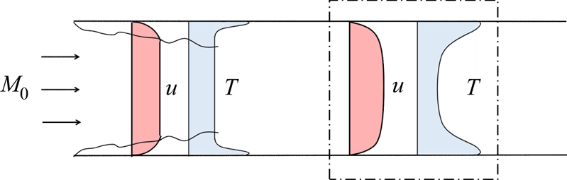
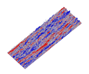
In the present study, the compressible turbulent channel flow with constant total mass, mass flux and heat flux is considered, as in Yu, Xu & Pirozzoli (Reference Yu, Xu and Pirozzoli2019). This physical model is designed to replicate the flow coming from a long wind tunnel at a nominal Mach number  $M_0$ as depicted in figure 1. The region of fully developed flow (highlighted by a dash–dotted box) is simulated. The mass and the mass flux are kept the same as the nominal inflow. The wall temperature is equal to the recovery temperature in the upstream flow. The uniformly distributed heat sink is added to balance the heat due to viscous friction. The governing equations for the compressible ideal Newtonian gas in a Cartesian coordinate system (
 $x_i$,
 $i=1$, 2, 3, also referred to as
 $x$,
 $y$,
 $z$ in the following) are written as
 $$\begin{gather} \frac{\partial{\rho}}{\partial{t}} + \frac{\partial{\rho u_j}} {\partial{ x_j}}=0 , \end{gather}$$
 $$\begin{gather}\frac{\partial {\rho u_i}} {\partial {t}} + \frac{\partial {\rho u_i u_j}} {\partial {x_j}} = - \frac{\partial {p}} {\partial {x_i}}+ \frac{\partial{\tau_{ij}}} {\partial {x_j}} + f_1 \delta_{i1}, \end{gather}$$
 $$\begin{gather}\frac{\partial{\rho E}}{\partial{t}}+\frac{\partial{\rho u_j E}}{\partial{x_j}} = -\frac{\partial{p u_j}}{\partial{x_j}}+ \frac{\partial{u_i \tau_{ij}}} {\partial {x_j}} - \frac{\partial{q_j}} {\partial{x_j}} +f_1 u_1 - \phi \end{gather}$$
with
 \begin{equation} p=\rho R T,\quad \tau_{ij}=2\mu S_{ij}-\frac{2}{3}\mu S_{kk} \delta_{ij}, \quad q_j= - \lambda \frac{\partial{T}}{\partial{x_j}}, \quad E = C_v T + \frac{1}{2}u_iu_i ,\end{equation}
where  $R$ is the gas constant,
 $C_v$ is the constant-volume specific heat,
 $\mu$ and
 $\lambda$ are the dynamic viscosity and the heat conduction coefficients, respectively, whose variation with temperature is considered by Sutherland's law. The body force
 $f_1$ is added in the streamwise momentum equation to ensure a constant mass flux. The heat source
 $\phi$ in the energy equation balances the viscous heating to maintain a constant bulk temperature as
 $T_b=0.25 T_0 + 0.75 T_r$, where
 $T_0$ and
 $T_r$ are the free stream temperature and the estimated recovery temperature in the upstream boundary layer. Periodic conditions are applied in the streamwise (
 $x$) and spanwise (
 $z$) directions. At the upper and lower walls, the no-slip and no-penetration conditions are applied for velocity, and the isothermal condition for temperature. By setting the wall temperature as the nominal recovery value
 $T_r$, the wall heat flux can be kept small enough to ensure its influence on near-wall dynamics is negligible (Yu et al. Reference Yu, Xu and Pirozzoli2019). The bulk Reynolds number is defined as
 $Re_b=\rho _b U_b h / \mu _{w}$ and the bulk Mach number as
 $M_b=U_b/\sqrt {\gamma R T_b}$, where the subscripts ’
 $b$’ and ’
 $w$’ denote the bulk and wall values, respectively.
Sketch of computational domain.

The ensemble average of a flow quantity  $\varphi$ is represented as
 $\bar \varphi$, and the corresponding fluctuations as
 $\varphi '$. The Favre average,
 $\overline {\rho \varphi } / \bar \rho$, is denoted as
 $\tilde \varphi$, and the corresponding fluctuation as
 $\varphi ''$. As in incompressible flow, the friction velocity
 $u_\tau$ is defined by the mean wall shear stress
 $\tau _w$, as
 \begin{equation} u_\tau=\sqrt{\frac{\tau_w} {\bar \rho_w} }, \quad \left.\tau_w= \mu_w \frac{\mathrm{d}\bar u}{\mathrm{d} y} \right|_w, \end{equation}
hence
 \begin{equation} Re_\tau = \frac{ \bar \rho_w u_\tau h}{\mu_w}, \quad u^+ = \frac{\bar u }{u_\tau}, \quad y^+ = \frac{y}{h} Re_\tau.\end{equation}
The open-source code Hoam-OpenCFD developed by Li, Fu & Ma (Reference Li, Fu and Ma2010) is employed to perform the DNS. The governing equations are numerically solved by the finite-difference method. The convective terms are discretized by the seventh-order upwind scheme and the viscous terms by the eighth-order central scheme. A third-order total variation diminishing Runge–Kutta scheme is used for time advancement. The physical parameters and numerical settings are listed in table 1. The recovery temperature relates to the upstream temperature as  $T_r=(1+(\gamma -1)rM^2_0/2)T_0$, with
 $r$ the recovery coefficient and
 $M_0$ the nominal Mach number. The friction Reynolds number under consideration is moderate, with the value of
 $Re_\tau =1170$. The size of the computational domain is large enough to contain VLSMs (Bernardini, Pirozzoli & Orlandi Reference Bernardini, Pirozzoli and Orlandi2014). The grids in streamwise and spanwise directions are uniformly distributed, and stretched by hyperbolic tangent function in the wall-normal direction. The mesh intervals are fine enough to resolve small-scale fluctuations for DNS. The simulation has been run for more than
 $1000h/U_b$ for statistical convergence.
Physical and computational parameter settings. Here  $Re_b$ and
 $Re_\tau$ are the bulk and friction Reynolds numbers;
 $M_0$,
 $M_b$ and
 $M_C$ are the upstream nominal, bulk and centreline Mach numbers;
 $T_w$ and
 $T_r$ are the wall and recovery temperatures;
 $L_{x_i}$,
 $N_{x_i}$ and
 $\Delta x_i$ denote the domain length, grid numbers and grid interval along the
 $x_i$ direction.

3. Superposition and modulation effects
3.1. Mean and variance of velocity and temperature
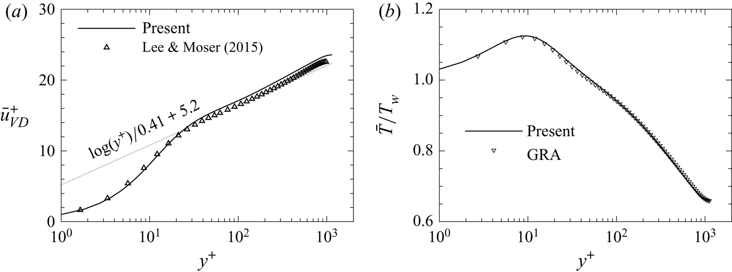
The mean velocity and temperature distributions are shown in figure 2. The Van Driest transformed mean velocity (Van Driest Reference Van Driest1951) is compared with that of the incompressible flow at a similar friction Reynolds number around  $Re_\tau \approx 1000$ (Lee & Moser Reference Lee and Moser2015) in figure 2(a). The profiles collapse well below the buffer layer. In the logarithmic layer the slopes are identical, whilst the intercept for the present compressible flow is slightly higher than the standard log-law and the incompressible flow. This is caused by the slight mean property gradient in the near-wall region (Modesti & Pirozzoli Reference Modesti and Pirozzoli2016; Trettel & Larsson Reference Trettel and Larsson2016), and has been illustrated in our previous study (Yu et al. Reference Yu, Xu and Pirozzoli2019). As shown in figure 2(b), the mean temperature distribution normalized by the wall temperature collapses well with the generalized Reynolds analogy proposed by Zhang et al. (Reference Zhang, Bi, Hussain and She2014) as
 \begin{equation} \frac{\bar T}{T_w} = 1 +\left(\left.\frac{\bar u_C}{T_w} \frac{\partial{\bar T }}{\partial{\bar u}}\right|_w \right) \frac{\bar u}{\bar u_C} + \left( \left.\frac{\bar T_C - T_w}{T_w} -\bar u_C \frac{\partial{\bar T}}{\partial{\bar u}}\right|_w \right) \frac{{\bar u}^2}{{\bar u_C}^2},\end{equation}
where the subscript  $C$ denotes the value at the channel centreline. This suggests that the extra heat source introduced in the energy equation does not invalidate the generalized Reynolds analogy in (3.1). The mean temperature profile first increases slightly with
 $y^+$ below the buffer layer, reaches maxima at
 $y^+ \approx 10$, then decreases above this location.
Distributions of mean velocity and temperature. (a) Mean velocity with Van Driest transformation, compared with the result by Lee & Moser (Reference Lee and Moser2015) at  $Re_\tau \approx 1000$ for incompressible flows, (b) mean temperature normalized by wall temperature, compared with the result of generalized Reynolds analogy given by equation (3.1).

The variances of velocity and temperature fluctuation normalized, respectively, by the friction velocity and wall temperature,
 \begin{equation} R^*_{u_i u_i}=\frac{\bar \rho \widetilde{ u''_i u''_i}}{\bar \rho_w u^2_\tau}, \quad R^+_{TT}=\frac{\overline{T'^2}}{T^2_w},\end{equation}
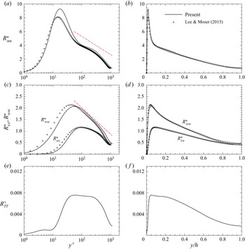
are shown in figure 3 in wall and global coordinates, respectively. For velocity fluctuations, the minor difference between the present and reference results in the inner region is attributed to the compressibility effects, which are only evident near the wall. In the outer region, the present results agree well with those of the incompressible flows. Specifically, figures 3(a) and 3(b) show the variance of the streamwise velocity fluctuation,  $R^*_{uu}$, plotted against the inner and outer scales, respectively. For the present compressible flow, the peak value is slightly higher than the referenced incompressible flow with the peak location farther away from the wall. In the logarithmic region adjacent to
 $y^+ \approx 100$, a logarithmic decay with approximately the same slope as those reported by Jimenez & Hoyas (Reference Jimenez and Hoyas2008) for incompressible flow is observed. The distribution of the present
 $R^*_{uu}$ agrees well with the incompressible flow above
 $y \approx 0.1h$, indicating that the compressibility effect on velocity variances is negligible in the outer region. As presented in figure 3(c,d), the variances of
 $v''$ and
 $w''$, namely
 $R^*_{vv}$ and
 $R^*_{ww}$, are lower than those of the incompressible flow in the near-wall region, while they collapse above
 $y \approx 0.1h$. The logarithmic decay of
 $R^*_{ww}$ adjacent to
 $y^+ \approx 100$ is similar to incompressible flows, and more prominent compared with
 $u''$. As for temperature, its variance
 $R^+_{TT}$ remains at a low level below
 $y^+ \approx 10$, then rapidly increases and reaches a peak around
 $y^+ \approx 40$. It remains nearly constant from
 $y^+ \approx 50$ to
 $y^+ \approx 300$, and gradually decreases in the outer region above
 $y \approx 0.3h$.
Distribution of velocity and temperature fluctuations variances with (a,c,e,g)  $y^+$ and (b,d, f,h)
 $y/h$; with (a,b)
 $R^*_{uu}$, (c,d)
 $R^*_{vv}$ and
 $R^*_{ww}$, (e, f)
 $R^+_{TT}$. Red dashed lines in (a) denote
 $R^*_{uu} = -1.15 \log (y/h)+2.5$ and in (c)
 $R^*_{ww} = -0.5 \log (y/h)+0.8$, respectively.

3.2. Superposition and modulation of LSMs on near-wall turbulence
Considering the peak positions of  $R^*_{uu}$ and
 $R^+_{TT}$, the instantaneous distribution of
 $u''$ at
 $y^+=15$ and
 $T'$ at
 $y^+=30$ in the near-wall region as well as those at
 $y=0.2h$ in the logarithmic region are shown in figure 4. The colour bands for temperature are reversed from those for velocity, considering the negative correlation between
 $T'$ and
 $u''$. The
 $u''$ at
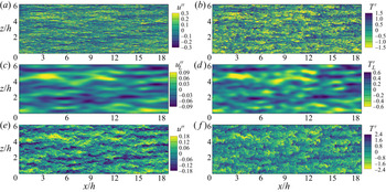
 $y^+=15$ shown in figure 4(a) are dominated by small-scale low-speed streaks caused by the ‘sweep’ and ‘ejection’ in the near-wall cycles (Jiménez & Moin Reference Jiménez and Moin1991; Hamilton, Kim & Waleffe Reference Hamilton, Kim and Waleffe1995; Jiménez & Pinelli Reference Jiménez and Pinelli1999; Duan Reference Duan2011; Lagha et al. Reference Lagha, Kim, Eldredge and Zhong2011). Moreover, large-scale streaky patterns are also looming. By applying spectral filtering at the cutoff wavelength of
 $\lambda _x=2h$ and
 $\lambda _z=0.5 h$, the large-scale portion of
 $u''$,
 $u''_L$, is obtained and shown in figure 4(c). The distribution of
 $u''_L$ at
 $y^+=15$ bears a remarkable resemblance to that at
 $y=0.2h$ shown in figure 4(e), where the large-scale streaky patterns with streamwise and spanwise scales of approximate
 $8h$ and
 $h$ are dominant. This indicates that the LSMs at
 $y=0.2h$ penetrate into the near-wall region and superposes on the near-wall small-scale fluctuations, leaving ‘footprints’ at
 $y^+=15$, as widely reported in incompressible (Hutchins & Marusic Reference Hutchins and Marusic2007a; Illingworth, Monty & Marusic Reference Illingworth, Monty and Marusic2018) and supersonic flows (Ganapathisubramani et al. Reference Ganapathisubramani, Clemens and Dolling2006; Pirozzoli & Bernardini Reference Pirozzoli and Bernardini2011, Reference Pirozzoli and Bernardini2013) at moderate and high Reynolds numbers.
Instantaneous distributions of (a)  $u''$ at
 $y^+=15$, (b)
 $T'$ at
 $y^+=30$, (c,d) the large-scale portion of fluctuations in (a,b) obtained by spectral filtering with the cutoff wavelength at
 $\lambda _x=2 h$ and
 $\lambda _z=0.5 h$, (e, f)
 $u''$ and
 $T'$ at
 $y=0.2h$.

The temperature fluctuation  $T'$ at
 $y^+=30$ shown in figure 4(b) also forms small-scale streaky patterns. Compared with those of
 $u''$, the
 $T'$ structures are less organized. The high-temperature regions are strongly correlated with the low-speed streaks, indicating a negative correlation between them (Duan Reference Duan2011; Pirozzoli & Bernardini Reference Pirozzoli and Bernardini2011). The corresponding large-scale portion
 $T'_L$, shown in figure 4(d), resembles those of the large-scale velocity
 $u''_L$ in figure 4(c), and can also be discerned in the temperature fluctuation
 $T'$ at
 $y=0.2h$. This confirms the close relation between the large-scale temperature and velocity fluctuations, as well as the existence of the superposition effect in the temperature field.
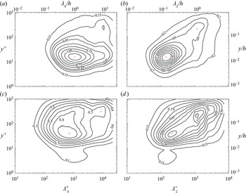
For a quantitative description of the superposition effect, we display in figure 5 the premultiplied streamwise and spanwise spectra of  $u''$ and
 $T'$ defined as
 \begin{equation} E^*_{uu}=\overline{\hat u^* \hat u^{*c}},\quad E^+_{TT}=\overline{\hat T^+ \hat T^{+c}}, \end{equation}
where  $\hat \cdot$ denotes the spectral coefficient, the superscript
 $c$ denotes its complex conjugate and
 \begin{equation} u^*=\frac{\sqrt{\rho} u''}{\sqrt{\rho_w} u_\tau},\quad T^+{=}\frac{T'}{T_w}.\end{equation}
The inner peaks of the velocity spectra lie at  $y^+ \approx 15$ with
 $\lambda _x^+ \approx 1000$ and
 $\lambda _z^+ \approx 120$, which are the typical length scales of the near-wall low-speed streaks (Jiménez et al. Reference Jiménez, Kawahara, Simens, Nagata and Shiba2005; Hwang Reference Hwang2013). Above
 $y^+=100$, there is an obvious trend for the appearance of another peak at
 $y \approx 0.2h$ with
 $\lambda _x \approx 8h$ and
 $\lambda _z \approx h$, consistent with those of the VLSMs (Kim & Adrian Reference Kim and Adrian1999; Hutchins & Marusic Reference Hutchins and Marusic2007a). These peaks will be more obvious with the increment of the Reynolds number, as reported by Smits et al. (Reference Smits, McKeon and Marusic2011) and Lee & Moser (Reference Lee and Moser2015). Notably, the peak at
 $\lambda _x = 8h$ and
 $\lambda _z = h$ penetrate downwards into the near-wall region until the viscous sublayer, which is the evidence of the imprinted ‘footprints’ of the VLSMs in the near-wall region. The distribution of temperature spectra differs from those of the velocity. The intensities of
 $T^+$ are low below
 $y^+=10$ resulting from the small mean-temperature gradient due to the quasi-adiabatic boundary condition. The inner peaks of the spectra lie at
 $y^+ \approx 40$ in the near-wall region with the streamwise and spanwise scales of
 $\lambda _x^+ \approx 1000$ and
 $\lambda _z^+ \approx 200$, respectively. The large-scale fluctuations of temperature are more prominent than those of velocity with an obvious peak at
 $y \approx 0.2h$ and
 $\lambda _z \approx h$ in the spanwise spectra. In the streamwise spectra, the peak in the outer layer is also more obvious than that of the velocity, and spectral intensity around
 $\lambda _x \approx 8h$ remains nearly constant from
 $y \approx 0.6h$ to
 $y \approx 0.03h$, or
 $y^+ \approx 600$ to
 $y^+ \approx 30$ in the viscous scale. This indicates that the superposition effects of the large-scale temperature fluctuations are significantly different from those of the velocity.
Premultiplied streamwise and spanwise spectra for  $u^*$ and
 $T^+$, (a)
 $k_x E^*_{uu}(k_x)$, (b)
 $k_z E^*_{uu}(k_z)$, (c)
 $k_x E^+_{TT}(k_x)$, (d)
 $k_z E^+_{TT}(k_z)$. The inner and outer peaks are marked with the purple crossings.

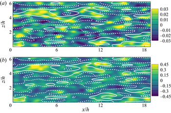
Besides the superposition effects, the LSM also interacts with the near-wall turbulence nonlinearly by increasing/decreasing its local fluctuation intensity (Hutchins & Marusic Reference Hutchins and Marusic2007b; Mathis et al. Reference Mathis, Hutchins and Marusic2009a,Reference Mathis, Monty, Hutchins and Marusicb). To visually display this amplitude modulation effect, the envelopes of the density-weighted small-scale velocity fluctuation  $u^*_s=u^*-u^*_L$ at
 $y^+=15$ and temperature fluctuation
 $T^+_s=T^+-T^+_L$ at
 $y^+=30$ are presented in figure 6 along with the large-scale velocity
 $u^*_L$. The envelopes of
 $u^*_s$ and
 $T^+_s$,
 $E(u^*_s)$ and
 $E(T^+_s)$, are obtained by Hilbert transformation as in Mathis et al. (Reference Mathis, Hutchins and Marusic2009a), with the mean values removed. By low-pass filtering the envelopes
 $E(u^*_s)$ and
 $E(T^+_s)$ at the same cutoff scales as those in
 $u^*$, the large-scale envelopes of
 $u^*_s$ and
 $T^+_s$ are obtained, denoted as
 $E_L(u^*_s)$ and
 $E_L(T^+_s)$, respectively. It is apparent that the regions of
 $E_L(u^*_s)>0$ and
 $E_L(T^+_s)>0$ align well with those of
 $u^*_L>0$, and vice versa. This confirms that the small-scale signals
 $u^*_s$ and
 $T^+_s$ are intensified/abated by the large-scale velocity
 $u^*_L$. The correlation coefficient between
 $u^*_L$ and
 $E_L(u^*_s)$ at
 $y^+=15$ is approximately
 $0.43$, and that between
 $u^*_L$ and
 $E_L(T^+_s)$ at
 $y^+=30$ is around
 $0.65$, indicating that the temperature fluctuations suffer stronger modulation than velocity by LSMs in the outer region.
Contours of (a)  $E'_L(u^*_s)$ at
 $y^+=15$ and (b)
 $E'_L(T^+_s)$ at
 $y^+=30$, white solid and dashed lines are
 $u^*_L=0.6$ and
 $-0.6$, respectively.

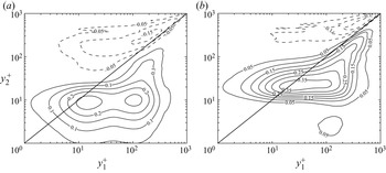
To quantitatively evaluate this modulation effect, the two-point correlation of  $u^*_L$ and
 $E_L(u^*_s)$ or
 $E_L(T^+_s)$ is employed: (Bernardini & Pirozzoli Reference Bernardini and Pirozzoli2011)
 $$\begin{gather} C^{uu}_{AM} (y^+_1, y^+_2) = \overline{u^*_L(y^+_1)E_L(u^*_s(y^+_2))}, \end{gather}$$
 $$\begin{gather}C^{uT}_{AM} (y^+_1, y^+_2) = \overline{u^*_L(y^+_1)E_L(T^*_s(y^+_2))}. \end{gather}$$
The results are presented in figure 7. For velocity, a peak at  $y^+_1 \approx 100$ and
 $y^+_2 \approx 10$ can be observed in figure 7(a), indicating that the large-scale velocity
 $u^*_L$ at
 $y^+_1 \approx 100$ has the strongest modulation effects on the near-wall small-scale motions at
 $y^+_2 \approx 10$. This map of two-point correlation resembles that reported in Bernardini & Pirozzoli (Reference Bernardini and Pirozzoli2011) for a supersonic turbulent boundary layer at
 $Re_\tau = 1000$ and
 $M=2$. The modulation effects on the other two velocity components are similar to the streamwise component (Talluru et al. Reference Talluru, Baidya, Hutchins and Marusic2014; Yao et al. Reference Yao, Huang and Xu2018), therefore they are not reported here. For temperature, high correlation appears around
 $y^+_1 = 10 \sim 100$ and
 $y^+_2 \approx 20$. Due to the quasi-adiabatic thermal boundary condition in the present study, the large-scale temperature fluctuation neither penetrates much deeper into the viscous sublayer as stated above (Pirozzoli & Bernardini Reference Pirozzoli and Bernardini2011), nor significantly modulates the small-scale motions there.
Distribution of (a)  $C^{uu}_{AM}$ and (b)
 $C^{uT}_{AM}$.

The above analysis reveals that the LSMs in compressible flow influence the near-wall turbulence via superposition and modulation as in incompressible flows. In the next section, the predictive model for compressible near-wall turbulence will be developed based on the MMH model (Mathis et al. Reference Mathis, Hutchins and Marusic2011) for velocity, and the SRA for temperature.
4. Predictive models
4.1. Predictive models for velocity fluctuation
The original MMH model (Marusic et al. Reference Marusic, Mathis and Hutchins2010; Mathis et al. Reference Mathis, Hutchins and Marusic2011) and its modified version by Baars et al. (Reference Baars, Hutchins and Marusic2016) can be written in a unified form, as follows:
 \begin{align} u^+_p(x^+,y^+,z^+)=u^+_u(x^+,y^+,z^+)(1+\varGamma_{uu}u^+_L(x^+ - \Delta x^+_{\varGamma_{uu}}, y^+, z^+))+u^+_L(x^+,y^+,z^+),\end{align}
with the subscript ‘ $p$’ denoting the predicted and ‘
 $u$’ the universal signal. In the original model proposed by Marusic et al. (Reference Marusic, Mathis and Hutchins2010), the
 $u^+_L$ was obtained from the large-scale signal at the centre of the logarithmic region
 $y^+_{O}=3.9\sqrt {Re_\tau }$ as
 \begin{equation} u^+_L(x^+,y^+,z^+)=\alpha_u u^+_L(x^+ + \Delta x^+, y^+_O,z^+).\end{equation}
The superposition coefficient  $\alpha _u$ and the phase shift
 $\Delta x^+$ are obtained a priori from the correlation of
 $u^+_L$ at
 $y^+$ and
 $y^+_O$. The modulation effect is taken into account by the modulation coefficient
 $\beta _u$, related to
 $\varGamma _{uu}$ by
 $\varGamma _{uu}=\beta _u / \alpha _u$. It is obtained by an iterative procedure to achieve a zero (trivial) value of
 $C_{AM} (u^+_L, E_L(u^+_u))$ (Mathis et al. Reference Mathis, Hutchins and Marusic2011). The ‘detrended’ and demodulated turbulent fluctuations are reckoned as the universal signal
 $u^+_u$. Note that the phase shift between the superposition and modulation was not considered by this model, i.e.
 $\Delta x^+_{\varGamma _{uu}}=0$. Baars et al. (Reference Baars, Hutchins and Marusic2016) revised the MMH model by using the sLSE to determine the superposed large-scale velocity
 $u^+_L$,
 \begin{equation} u^+_L(x^+,y^+,z^+)=\mathscr{F}^{-1}_x \{ \hat H_{uu}(\lambda_x^+,y^+) \mathscr{F}_x \{ u^+_L(x^+,y^+_O,z^+)\}\},\end{equation}
with  $\mathscr {F}_x$ and
 $\mathscr {F}^{-1}_x$ denoting the operators of Fourier and inverse Fourier transformation in the streamwise direction.
 $\hat H_{uu}$ is the complex-valued kernel function at streamwise wavelength
 $\lambda ^+_x$ and wall-normal direction
 $y^+$, obtained as
 \begin{equation} \hat H_{uu}(\lambda_x^+,y^+) = \frac{\overline{\hat u(\lambda_x^+,y^+) \hat u^c(\lambda_x^+,y^+_O)}} {\overline{\hat u(\lambda_x^+,y^+_O) \hat u^c(\lambda_x^+,y^+_O)}}. \end{equation}
Moreover, the phase shift between the superposition and modulation was considered using the results reported in Baars et al. (Reference Baars, Talluru, Hutchins and Marusic2015).
The predictive model proposed by Agostini & Leschziner (Reference Agostini and Leschziner2016b) (AL model), covers all the three velocity components. The superposition coefficients  $\alpha _{u_i}$ are obtained by the ratio between the fluctuation intensity of the large-scale signals at
 $y^+$ and
 $y^+_O$ with near-wall modification, i.e.
 \begin{equation} \alpha_{u_i}=\psi \frac{\sqrt{\overline{u'^2_{iL}}}(y^+)}{\sqrt{\overline{u'^2_{iL}}}(y^+_O)}, \end{equation}
where  $\psi =y^+/13.5$ when
 $y^+ \le 13.5$ and
 $\psi =1$ otherwise. The splatting-induced distortion is also considered in the modulation (Agostini et al. Reference Agostini, Leschziner and Gaitonde2016) by separately determining the modulation effects on the upper and lower envelopes of the small-scale fluctuations.
The predictive models proposed by Yin et al. (Reference Yin, Huang and Xu2018) utilized the turbulent fluctuations in the minimal flow units as the universal signal. This model combined the advantages of the MMH model and the AL model, involving all the three velocity components and the splatting distortion in the prediction of the streamwise velocity. Herein, we start off from this model to develop the predictive model for the present compressible velocity fluctuations. Considering that the compressibility effects on velocity fluctuations can be greatly reduced when weighted by density as in (3.2a,b) (Duan Reference Duan2011), the density variation should be taken into account for achieving Mach number independence. In the predictive model by Helm & Martin (Reference Helm and Martin2013), the local mean density is only involved in the universal signal, while the large-scale portion is unaffected. In the present model, we adopt an alternative strategy in which the density-weighted velocity fluctuation  $u^*_i(=\sqrt { \rho / \rho _w} u^+_i)$ is predicted instead of
 $u^+_i(=u''_i/u_\tau )$. This is based on the observation that the fluctuation variances and spectra collapse better at different Mach numbers for the density-weighted velocity fluctuations. In so doing, the models are expected to be less Mach number dependent (refer to the Appendix for validation). According to Yin et al. (Reference Yin, Huang and Xu2018), the predictive models for
 $u^*_i$ are thus expressed as
 \begin{align}& u^*_{p}(x^+,y^+,z^+)\nonumber\\ & = \left\{\begin{array}{@{}ll} u^*_u(x^+,y^+,z^+)
(1+\varGamma_{uu^+}(y^+) u^*_L(x^+ -\Delta
x^+_{\varGamma_{uu}},y^+,z^+))+ u^*_L(x^+,y^+,z^+), & u^*_u
\ge 0,\\ u^*_u(x^+,y^+,z^+) (1+\varGamma_{uu^-}(y^+)
u^*_L(x^+ -\Delta x^+_{\varGamma_{uu}},y^+,z^+))+
u^*_L(x^+,y^+,z^+), & u^*_u < 0, \end{array}
\right. \end{align}
 $$\begin{align} v^*_{p}(x^+,y^+,z^+)&= v^*_u(x^+,y^+,z^+)(1+\varGamma_{uv}(y^+) u^*_L(x^+ -\Delta x^+_{\varGamma_{uv}},y^+,z^+))\nonumber\\ &\quad + v^*_L(x^+,y^+,z^+), \end{align}$$
 $$\begin{align}w^*_{p}(x^+,y^+,z^+)&= w^*_u(x^+,y^+,z^+)(1\!+\!\varGamma_{uw}(y^+) u^*_L(x^+ -\Delta x^+_{\varGamma_{uw}},y^+,z^+))\nonumber\\ &\quad + w^*_L(x^+,y^+,z^+). \end{align}$$
In the prediction of the streamwise velocity component, the modulation effects on the upper and lower envelopes,  $\varGamma _{uu^+}$ and
 $\varGamma _{uu^-}$, are considered separately, as expressed in (4.6). The large-scale streamwise component
 $u^*_L$ is obtained by sLSE as in Baars et al. (Reference Baars, Hutchins and Marusic2016), while the wall-normal and spanwise components,
 $v^*_L$ and
 $w^*_L$, are obtained as those in the AL model (Agostini & Leschziner Reference Agostini and Leschziner2016b) by linear mapping. The modulation coefficients for each component are determined separately. Details will be introduced in § 5.1.
4.2. Predictive model for temperature fluctuation
As for the prediction of temperature, Helm & Martin (Reference Helm and Martin2014) proposed a model similar to the MMH model for velocity,
 \begin{equation} T_p=T_u(y^+)(1+\beta_T u^+_L(y^+_O,\theta))+\alpha_T T_L(y^+_O,\theta_T),\end{equation}
where  $\theta$ and
 $\theta _T$ represent the inclination angle of the large-scale structure of velocity and temperature. Although this formula seems plausible, its consistency with the SRA is inconclusive. Herein, instead of presuming it as an empirical formula as velocity, we derive the predictive model based on the refined SRA proposed by Gaviglio (Reference Gaviglio1987), namely the ‘Gaviglio strong Reynolds analogy’ (GSRA). We assume that the temperature and velocity fluctuations can be related as
 \begin{equation} T' \approx \frac{\tilde u}{C_p (\partial \bar T_t / \partial \bar T -1)} u'' \end{equation}
or equivalently as (Zhang et al. Reference Zhang, Bi, Hussain and She2014)
 \begin{equation} T' \approx \frac{\partial \bar T}{\partial \tilde u} u'',\end{equation}
where  $\bar T_t = \bar T + \tilde u^2 / (2 C_p)$ represents the mean total temperature. If the large- and small-scale velocity and temperature fluctuations equally satisfy the GSRA, it can be expressed as the summation of large- and small-scale fluctuations:
 $$\begin{gather} T' =T'_L+T'_s, \end{gather}$$
 $$\begin{gather}T'_L \approx \frac{\partial \bar T}{\partial \tilde u} u''_L, \end{gather}$$
 $$\begin{gather}T'_s \approx \frac{\partial \bar T}{\partial \tilde u} u''_s. \end{gather}$$
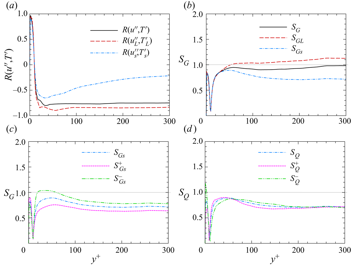
To verify this postulation, we firstly present the correlation coefficients between velocity and temperature fluctuations,  $R(u'',T')$,
 $R(u''_L,T'_L)$ and
 $R(u''_s,T'_s)$ in figure 8(a). For
 $R(u'',T')$, it varies from positive to negative at
 $y^+\approx 10$, and remains at almost a constant value of
 $-0.75$ above
 $y^+=20$. The correlation for large-scale fluctuations,
 $R(u''_L,T'_L)$, varies with
 $y^+$ similarly as
 $R(u'',T')$, whilst the higher constant value of
 $-0.85$ above
 $y^+=20$ insinuates the stronger correlation between them. As for the small-scale fluctuations, the correlation
 $R(u''_s,T'_s)$ is also negative above
 $y^+=20$. It is approximately
 $-0.5$ at
 $y^+=20$ and varies monotonically with
 $y^+$ and attains
 $-0.2$ at
 $y^+=300$, showing a weaker correlation between
 $u''_s$ and
 $T'_s$. This, in one way, indicate that the SRA may not be suitable to directly relate the small-scale velocity and temperature fluctuations.
Validation for the SRA, (a) correlation coefficients  $R(u'',T')$,
 $R(u''_L,T'_L)$ and
 $R(u''_s,T'_s)$, (b) ratios
 $S_Q$,
 $S_{GL}$ and
 $S_{Gs}$, (c) ratios
 $S_{Gs}$,
 $S^+_{Gs}$ and
 $S^-_{Gs}$, (d) ratio
 $S_Q$ defined in (4.15) and
 $S^+_Q$ and
 $S^-_Q$. The superscripts ‘
 $+$’ and ‘
 $-$’ denote the conditional average in the region
 $u''_L> u_t$ and
 $u''_L<- u_t$, respectively.

We further evaluate the validity of GSRA for large- and small-scale motions by the ratios defined as
 \begin{equation} S_G= \frac{\partial \bar T}{\partial \tilde u} \frac{\sqrt{\overline{u''^2}}}{\sqrt{\overline{T'^2}}},\quad S_{GL}= \frac{\partial \bar T}{\partial \tilde u} \frac{\sqrt{\overline{u''^2_L}}}{\sqrt{\overline{T'^2_L}}},\quad S_{Gs}= \frac{\partial \bar T}{\partial \tilde u} \frac{\sqrt{\overline{u''^2_s}}}{\sqrt{\overline{T'^2_s}}}. \end{equation}
The results are displayed in figures 8(b). The ratios  $S_G$ and
 $S_{GL}$ are both approximately 1.0, proving that GSRA provides accurate fluctuation intensities for
 $T'$ and
 $T'_L$. The ratio
 $S_{Gs}$, on the other hand, is significantly lower than
 $1.0$. Specifically, within large-scale extreme high- and low-speed regions, i.e.
 $u''_L> u_t$ and
 $u''_L<- u_t$, with
 $u_t= \sqrt {\overline {u''^2_L}}$, the conditionally averaged ratios, denoted by
 $S^+_{Gs}$ and
 $S^-_{Gs}$, respectively, differ greatly above
 $y^+=20$, as shown in figure 8(c). This indicates that the impact of the large-scale velocity
 $u''_L$ on small-scale fluctuations, possibly due to the modulation effects, invalidates the previous assumption that the GSRA is equally satisfied by the small-scale fluctuations as by the large-scale fluctuations.
To remedy this defect, we propose the following modification based on the QSQH hypothesis (Zhang & Chernyshenko Reference Zhang and Chernyshenko2016) by incorporating the local large-scale fluctuations as
 \begin{equation} T'_s \approx \frac{\partial_y \bar T+ \partial_y T'_L}{\partial_y \tilde u +\partial_y u''_L}u''_s. \end{equation}
Accordingly, the following ratio  $S_Q$ is defined to validate this modified GSRA:
 \begin{equation} S_Q= \frac{\partial_y \bar T+ \partial_y T'_L}{\partial_y \tilde u +\partial_y u''_L} \frac{\sqrt{\overline{u''^2_s}}}{\sqrt{\overline{T'^2_s}}}.\end{equation}
The statistical results are presented in figure 8(d), along with the conditional average within the large-scale high- and low-speed regions, denoted as  $S^+_Q$ and
 $S^-_Q$, respectively. Compared with
 $S^+_{Gs}$ and
 $S^-_{Gs}$ in figure 8(c),
 $S^+_Q$ and
 $S^-_Q$ are collapsed well, indicating that the proposed formula (4.14) successfully eliminates the impact of large-scale signals.
Furthermore, expressing  $u''_s$ as the amalgamation of universal signals and modulation coefficients as
 $u''_s = (1+\varGamma _{uu} u^*_L) u_u$ and substituting into (4.14), the small-scale temperature fluctuations can be written as
 \begin{equation} T'_s \approx \frac{\partial \bar T }{\partial \tilde u} F(u''_L,T'_L) (1+\varGamma_{uu} u^*_L) u_u,\end{equation}
with
 \begin{equation} F(u''_L,T'_L)= \frac{\partial_y \bar T+ \partial_y T'_L} {\partial_y \tilde u +\partial_y u''_L} \frac{\partial \tilde u }{\partial \bar T} =\frac{1}{1 +\partial u''_L/ \partial \tilde u} \left( 1 + \frac{\partial T'_L}{\partial \bar T} \right). \end{equation}
Considering the GSRA for large-scale temperature fluctuations in (4.12) and assuming  $r_l = (\partial \bar T_t / \partial \bar T -1) = (\tilde u / C_p)(\partial \tilde u / \partial \bar T)$ to be constant (Zhang et al. Reference Zhang, Bi, Hussain and She2014), we have the following derivation:
 \begin{align} F(u''_L,T'_L) &=\frac{1}{1 +\partial u''_L/ \partial \tilde u} \left(1 + \frac{1}{r_l C_p}\frac{ \partial (\tilde u u''_L) }{\partial \bar T}\right)\nonumber\\ & = 1+\frac{\partial \tilde u /\partial \bar T} {r_l C_p (1+\partial u''_L / \partial \tilde u)}u''_L. \end{align}
Substituting (4.18) back into (4.16), we have
 \begin{equation} T'_s \approx \frac{\partial \bar T }{\partial \tilde u} (1+\varGamma_{uu} u^*_L) (1+\varGamma_{uT}u^*_L) u_u,\end{equation}
where
 \begin{equation} \varGamma_{uT}=\frac{u_\tau \partial \tilde u / \partial \bar T} {r_l C_p (1+ \partial u''_L/\partial \tilde u)}.\end{equation}
Considering that the universal velocity and temperature signals are related independently of LSM, the universal temperature fluctuation  $T_u$ may be written as
 \begin{equation} T_u \approx \frac{\partial \bar T }{\partial \tilde u} u_u,\end{equation}
henceforth,  $T'_s$ can be expressed as
 \begin{equation} T'_s=(1+\varGamma_{uu} u^*_L)(1+\varGamma_{uT} u^*_L) T_u.\end{equation}
This equation suggests that the small-scale temperature fluctuation is modulated by the large-scale velocity  $u''_L$ in the form of a quadratic function, instead of a simple linear function as in the predictive model of velocity. Since the formula is derived based on GSRA, it is expected to be applicable to other Mach numbers, at least where the GSRA is still valid (Yu & Xu Reference Yu and Xu2021).
Based on the above discussions, the predictive model for near-wall temperature fluctuations, incorporating the superposition, modulation, splatting-induced distortion and the phase shift between superposition and modulation, is proposed as
 \begin{align}& T^+_{p}(x^+,y^+,z^+)\nonumber\\ & \quad = \left\{\begin{array}{@{}ll}
T^+_u(x^+,y^+,z^+)(1+\varGamma_{uu^-}(y^+)u^*_L(x^+ -\Delta
x^+_{\varGamma_{uu}},y^+,z^+)) (1\\ \quad
+\varGamma_{uT^+}(y^+)u^*_L(x^+ -\Delta
x^+_{\varGamma_{uT}},y^+,z^+)) + T^+_L(x^+,y^+,z^+), &
T^+_u \ge 0,\\
T^+_u(x^+,y^+,z^+)(1+\varGamma_{uu^+}(y^+)u^*_L(x^+ -\Delta
x^+_{\varGamma_{uu}},y^+,z^+)) (1\\ \quad
+\varGamma_{uT^-}(y^+)u^*_L(x^+ -\Delta
x^+_{\varGamma_{uT}},y^+,z^+)) + T^+_L(x^+,y^+,z^+), &
T^+_u < 0. \end{array} \right.
\end{align}
The large-scale signal  $T^+_L$ is obtained by sLSE. The splatting-induced distortion is considered by the different modulation coefficients on the upper and lower envelopes, respectively. Note that the modulations on the upper and lower envelopes of velocity and temperature are reversed due to their negative correlation. The parameter calibrations will be further discussed in detail in subsequent sections.
5. Model parameters and universal signals
5.1. Model parameters
According to the presently proposed predictive model in (4.6)–(4.8) for velocity and (4.23) for temperature, the modulation coefficients  $\varGamma _{u \varphi }$ and the phase shift between modulation and superposition
 $\Delta x_{\varGamma _{u \varphi }}$ as well as the universal signals
 $\varphi _u$ must be predetermined, where
 $\varphi$ denotes
 $u$,
 $v$,
 $w$ or
 $T$, respectively.
We firstly consider the determination of the large-scale signals. The  $u^*_L$ and
 $T^+_L$ are obtained by sLSE, as in Baars et al. (Reference Baars, Hutchins and Marusic2016) and Yin et al. (Reference Yin, Huang and Xu2018), as
 $$\begin{gather} u^*_L(x^+,y^+,z^+)=\mathscr{F}^{-1}_x \{ \hat H_{uu}(\lambda_x^+,y^+) \mathscr{F}_x \{ u^*_L(x^+,y^+_O,z^+)\}\}, \end{gather}$$
 $$\begin{gather}T^+_L(x^+,y^+,z^+)=\mathscr{F}^{-1}_x \{ \hat H_{TT}(\lambda_x^+,y^+) \mathscr{F}_x \{ T^+_L(x^+,y^+_O,z^+)\}\}, \end{gather}$$
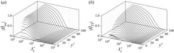
which recover the linear coherence between the LSMs in the inner and outer regions. The moduli of the kernel functions  $|\hat H_{uu}|$ and
 $|\hat H_{TT}|$ within the near-wall region are shown in figure 9. The present
 $|\hat H_{uu}|$ distribution is similar to those of the incompressible flows reported by Baars et al. (Reference Baars, Hutchins and Marusic2016) and Yin et al. (Reference Yin, Huang and Xu2018). It increases and approaches a nearly constant value for the large-scale portion as
 $y^+$ increases, and decreases sharply in the viscous sublayer and wavelength
 $\lambda _x^+ < 10^3$. A small plateau, not obviously manifested due to the limitation of the computational domain, is evidenced for large-scale motions around
 $\lambda ^+_x \gtrsim 5000$ above
 $y^+ \approx 15$. The distribution of
 $|\hat H_{TT}|$ is similar to that of
 $|\hat H_{uu}|$, except that it decays much more slowly for the small-scale motions at
 $\lambda _x^+ < 10^3$. This implies that the averaged slope of the structures of temperature fluctuations may be steeper than that of the velocity.
Distribution of (a)  $|\hat H_{uu}|$ and (b)
 $|\hat H_{TT}|$.

As for the other two velocity components,  $v^*_L$ and
 $w^*_L$ at different
 $y^+$ are obtained by linear mapping, as in Agostini & Leschziner (Reference Agostini and Leschziner2016b) and Yin et al. (Reference Yin, Huang and Xu2018), as
 $$\begin{gather} v^*_L(x^+,y^+,z^+)=\alpha_v(y^+) v^*_L(x^+ + \Delta x^+, y^+_O, z^+), \end{gather}$$
 $$\begin{gather}w^*_L(x^+,y^+,z^+)=\alpha_w(y^+) w^*_L(x^+ + \Delta x^+, y^+_O, z^+), \end{gather}$$
where the phase shift  $\Delta x^+$ is obtained as in (4.2). The superposition coefficients
 $\alpha _v$ and
 $\alpha _w$ are calculated by the ratio of root mean square of the large-scale fluctuation at
 $y^+$ and the centre of logarithmic region
 $y^+_O$,
 \begin{equation} \alpha_v(y^+)=\frac{\sqrt{\overline{v^{*2}_L}}(y^+)}{\sqrt{\overline{v^{*2}_L}}(y^+_O)}, \quad \alpha_w(y^+)=\frac{\sqrt{\overline{w^{*2}_L}}(y^+)}{\sqrt{\overline{w^{*2}_L}}(y^+_O)}. \end{equation}
Herein, the cutoff wavelengths in the streamwise and spanwise directions are selected as  $\lambda _x=2h$ and
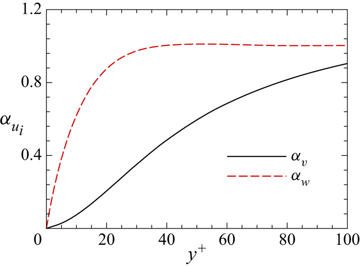
 $\lambda _z=0.5h$, respectively. The results are shown in figure 10. The superposition coefficient
 $\alpha _v$ increases monotonically with
 $y^+$, while
 $\alpha _w$ increases below
 $y^+=30$ and remains a constant value above it. Notably, although the universal and the large-scale signals are sensitive to the selection of the cutoff wavelength, the predicted results are robust against it.
Superposition coefficients  $\alpha _v$ and
 $\alpha _w$.

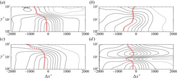
Secondly, we determine the phase shift between the modulation and superposition by calculating the two-point correlation between  $u^*_L$ and the envelope of the small-scale signal
 $\varphi _s = \varphi - \varphi _L$ defined as
 \begin{equation} R_{AM} (u^*_L, \varphi_s)= \frac{\overline{u^*_L(x^+ + \Delta x^+, y^+)E_L(\varphi_s (x^+,y^+))}} {\sqrt{\overline{u^{*2}_L}} \sqrt{\overline{E^2_L(\varphi_s)}} }. \end{equation}
The results are presented in figure 11. The maxima at each location, marked with red symbols in figure 11, are used to determine the phase shift  $\Delta x^+_{\varGamma _{u\varphi }}$ (Baars et al. Reference Baars, Hutchins and Marusic2016). In the spanwise direction, the phase shift is not considered due to the statistical homogeneity and symmetry (Yin et al. Reference Yin, Huang and Xu2018).
Two-point correlations defined in (5.6), (a)  $R_{AM} (u^*_L, u^*_s)$, (b)
 $R_{AM} (u^*_L, v^*_s)$, (c)
 $R_{AM} (u^*_L, w^*_s)$, (d)
 $R_{AM} (u^*_L, T^+_s)$. The maxima along the
 $\Delta x^+$ direction at each wall-normal location are marked with red symbols.

Lastly, the modulation coefficients and the universal signals are obtained simultaneously. In the previous studies (Marusic et al. Reference Marusic, Mathis and Hutchins2010; Mathis et al. Reference Mathis, Hutchins and Marusic2011; Baars et al. Reference Baars, Hutchins and Marusic2016, etc.), the modulation coefficient  $\varGamma _{u\varphi }$ is obtained by an iteration procedure to guarantee a zero correlation between the envelope of the universal signal
 $\varphi _u$ and the large-scale velocity
 $u^*_L$, i.e.
 $R_{AM} (u^*_L, \varphi _u)=0$. This iterative procedure is computationally expensive. In the present study, we developed an alternative strategy based on QHQS hypothesis. According to the predictive model, the small-scale signal can be expressed as
 $\varphi _{s}=\varphi _u(1+\varGamma _{u\varphi }u^*_L)$, therefore
 \begin{equation} \overline{\varphi^2_s}=\overline{\varphi^2_u} + 2\varGamma_{u\varphi} \overline{ u^*_L \varphi^2_u} + \varGamma^2_{u\varphi} \overline{u^{*2}_L \varphi^2_u}. \end{equation}
Within the extreme large-scale high/low-speed regions, we may expect and have validated by the present DNS that the conditional mean value of the large-scale velocity is much higher than the corresponding fluctuations, i.e.  $|\overline {u^*_L}| \gg |{u^*_L}'|$,
 $|\overline {u^{*2}_L}| \gg |{u^{*2}_L}'|$. Henceforth, the conditionally averaged variances in extreme large-scale high- and low-speed regions can be approximated as
 $$\begin{gather} \overline{\varphi^2_s} |_+ \approx \overline{\varphi^2_u} ( 1+2\varGamma_{u\varphi} \overline{u^*_L}|_+ +\varGamma^2_{u\varphi} \overline{u^{*2}_L}|_+ ), \end{gather}$$
 $$\begin{gather}\overline{\varphi^2_s} |_- \approx \overline{\varphi^2_u} ( 1+2\varGamma_{u\varphi} \overline{u^*_L}|_- +\varGamma^2_{u\varphi} \overline{u^{*2}_L}|_- ), \end{gather}$$
by neglecting the cross-correlations between  ${u^*_L}'$ and
 $\varphi _u$ on the right-hand side of (5.7). The ratio between (5.8) and (5.9), free of the influence of universal signal
 $\varphi _u$ gives an algebraic equation,
 \begin{equation} \frac{\overline{\varphi^2_s} |_+}{\overline{\varphi^2_s} |_-} \approx \frac{1+2\varGamma_{u\varphi}\overline{u^*_L}|_+ +\varGamma^2_{u\varphi}\overline{u^{*2}_L}|_+} {1+2\varGamma_{u\varphi}\overline{u^*_L}|_- +\varGamma^2_{u\varphi}\overline{u^{*2}_L}|_-},\end{equation}
with the only unknown quantity, being the modulation coefficient. Considering the splatting-induced distortions, the positive and negative  $u^*_s$ and
 $T^+_s$ are considered separately to obtain the modulation coefficients on the upper and lower envelopes.
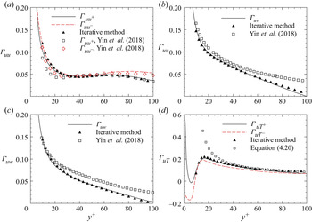
The thus obtained modulation coefficients are displayed in figure 12. The results for incompressible turbulence in Yin et al. (Reference Yin, Huang and Xu2018), and those obtained by the iterative method, are also displayed for comparison and validation. Note that only the upper envelopes for  $u^*$ and
 $T^+$ are calculated by the iterative method. The modulation coefficients of the upper and lower envelope of
 $u^*$, i.e.
 $\varGamma _{uu^+}$ and
 $\varGamma _{uu^-}$, collapse well with the incompressible results above
 $y^+=30$, whilst the present results are slightly higher below that location. The modulation coefficient
 $\varGamma _{uu^+}$ also collapses with the result obtained by the iterative method, proving the validity of the present method. The modulation effects of upper and lower envelopes
 $\varGamma _{uu^+}$ and
 $\varGamma _{uu^-}$ differ slightly, suggesting the insignificance of the asymmetrical modulation caused by the splatting-induced distortion. As for the other two velocity components, the presently obtained modulation coefficients
 $\varGamma _{uv}$ and
 $\varGamma _{uw}$ are lower than those of the incompressible flows, while collapse well with those by the iterative method. The modulation coefficients of temperature
 $\varGamma _{uT^+}$ and
 $\varGamma _{uT^-}$ are shown in figure 12(d). Below
 $y^+ \approx 10$, the difference between
 $\varGamma _{uT^+}$ and
 $\varGamma _{uT^-}$ is prominent. Above
 $y^+ \approx 10$, the modulation coefficient on the upper envelope
 $\varGamma _{uT^+}$ is merely slightly higher than those of the lower envelope
 $\varGamma _{uT^-}$ by no more than
 $20\,\%$. They also nearly collapse with the theoretical results in (4.20) above
 $y^+=30$. The inconsistency below
 $y^+=30$ is caused by the invalidity of the GSRA within the buffer layer, as discussed by Zhang et al. (Reference Zhang, Bi, Hussain and She2014).
Modulation coefficients, (a)  $\varGamma _{uu}$, (b)
 $\varGamma _{uv}$, (c)
 $\varGamma _{uw}$ and (d)
 $\varGamma _{uT}$, compared with the results in Yin et al. (Reference Yin, Huang and Xu2018) (hollow symbols) and by the iterative method (filled symbols).

5.2. Validation of the universal signal
According to the predictive models, the universal signals can be determined as
 $$\begin{gather} u^*_u=\frac{u^*(x^+,y^+,z^+)-u^*_L(x^+,y^+,z^+)} {1+\varGamma_{uu}u^*_L(x^+ - \Delta x^+_{\varGamma_{uu}},y^+,z^+)}, \end{gather}$$
 $$\begin{gather}v^*_u=\frac{v^*(x^+,y^+,z^+)-v^*_L(x^+,y^+,z^+)} {1+\varGamma_{uv}u^*_L(x^+ - \Delta x^+_{\varGamma_{uv}},y^+,z^+)}, \end{gather}$$
 $$\begin{gather}w^*_u=\frac{w^*(x^+,y^+,z^+)-w^*_L(x^+,y^+,z^+)} {1+\varGamma_{uw}u^*_L(x^+ - \Delta x^+_{\varGamma_{uw}},y^+,z^+)}, \end{gather}$$
 $$\begin{gather}T^+_u=\frac{T^+(x^+,y^+,z^+)-T^+_L(x^+,y^+,z^+)} {(1+\varGamma_{uu}u^*_L(x^+ - \Delta x^+_{\varGamma_{uu}},y^+,z^+)) (1+\varGamma_{uT}u^*_L(x^+ - \Delta x^+_{\varGamma_{uT}},y^+,z^+))}, \end{gather}$$
with the model parameters obtained in the previous section. The correlations between the envelope of the obtained universal signals and the large-scale velocity  $R_{AM}(u^*_L, \varphi _u)$ are checked. The correlation coefficients below
 $y^+<100$ are no more than
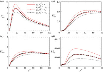
 $0.03$ in magnitude, proving that the universal signals are indeed demodulated. As a verification of its ‘universality’, we present the fluctuation variances and joint p.d.f. The conditionally averaged fluctuation variances of the small-scale and universal signals amid the extreme large-scale low- and high-speed regions are shown in figure 13. The conditionally averaged small-scale variances are different due to the modulation effect, higher in the large-scale high-speed region and lower in the large-scale low-speed region. This is consistent with the results by Agostini & Leschziner (Reference Agostini and Leschziner2016a). On the other hand, the conditionally averaged variances of the universal signals collapse with each other, suggesting that the universal signal is free from the modulation effects (Yin et al. Reference Yin, Huang and Xu2018).
Conditionally averaged fluctuation variances of velocity and temperature, normalized by viscous scales, (a)  $R^*_{uu}$, (b)
 $R^*_{vv}$, (c)
 $R^*_{ww}$, (d)
 $R^+_{TT}$.

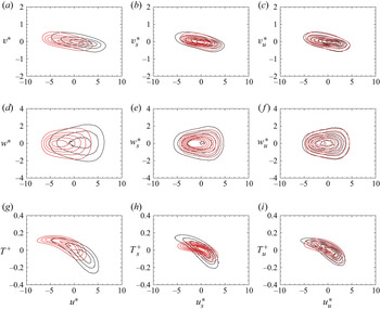
The conditionally averaged joint p.d.f.s in the regions of  $u''_L > u_t$ and
 $u''_L < -u_t$ between the streamwise velocity
 $u^*$ and the original signal
 $\varphi$,
 $P(u^*,\varphi )$, the small-scale signal
 $P(u^*_s,\varphi _s)$ and the universal signal
 $P(u^*_u,\varphi _u)$ at
 $y^+=15$ for velocity and
 $y^+=30$ for temperature are shown in figure 14, respectively. Figure 14(a,d,g) displays
 $P(u^*,\varphi )$. The centres of the p.d.f.s lie at different locations in the region of
 $u^*>0$ and
 $u^*<0$, respectively, due to the included LSMs. By removing the superposition of the LSMs (figure 14b,e,h), the centres of the p.d.f.s are located near the origin. However, owing to the modulation effects, the shapes of the p.d.f.s are more widely spread within the large-scale high-speed regions than those within the large-scale low-speed regions. Especially for
 $P(u^*_s,T^+_s)$, the inclination angle of the ‘tear-drop’ shaped p.d.f.s differs vastly. This is consistent with the previous conclusions in § 4 that the correlation between the small-scale velocity
 $u^*_s$ and temperature
 $T^+_s$ are highly different in large-scale high- and low-speed regions (recall figure 8a). By demodulation procedures (figure 14c, f,i), the joint p.d.f.s of the universal signals within the large-scale high- and low-speed regions are nearly identical, further indicating that the modulation effects are successfully removed. Particularly, the insignificant difference in
 $P(u^*_u,T^+_u)$ distributions further proves our presumption in § 4 that the universal signals of temperature and streamwise velocity are related independent of the LSMs.
Conditionally averaged joint p.d.f.s. Black lines,  $u_L > u_t$; red lines,
 $u_L < -u_t$. (a,d,g) Original signals, (b,e,h) small-scale signals, (c, f,i) universal signals, (a–c)
 $P(u^*,v^*)$ at
 $y^+=15$, (d–f)
 $P(u^*,w^*)$ at
 $y^+=15$, (g–i)
 $P(u^*,T^+)$ at
 $y^+=30$.

In this section, we have presented the methods and results to extract the universal signal from the raw DNS database. Specifically, an algebraic method to determine the modulation coefficients without the iterative procedures is proposed and validated. The extracted universal signals are further examined, which are found to be free from the superposition and modulation effects of the LSMs. The parameters and universal signals obtained in this section will be utilized to validate the proposed predictive model in § 6.
6. Prediction of near-wall velocity and temperature fluctuations
In this section, we validate the proposed predictive model in (4.6)–(4.8) and (4.23) for near-wall velocity and temperature fluctuations. As introduced in § 5.1, the superposition of large-scale signals on the near-wall region is obtained by sLSE for streamwise velocity  $u^*_L$ and temperature
 $T^+_L$, and by linear mapping for the wall-normal and spanwise velocity
 $v^*_L$ and
 $w^*_L$. We also utilize the modulation coefficients and the phase shift between superposition and modulation in § 5.1 and the extracted universal signal validated in § 5.2. During this procedure, the instantaneous large-scale signals and the universal signals are mingled in time for a better validation – to wit, the large-scale signal obtained at time
 $t_i$ is combined with the universal signal at time
 $t_j$ (
 $t_j \ne t_i$) for the prediction. The predicted results are evaluated by comparing the fluctuation variances and joint p.d.f.s with the corresponding DNS results.
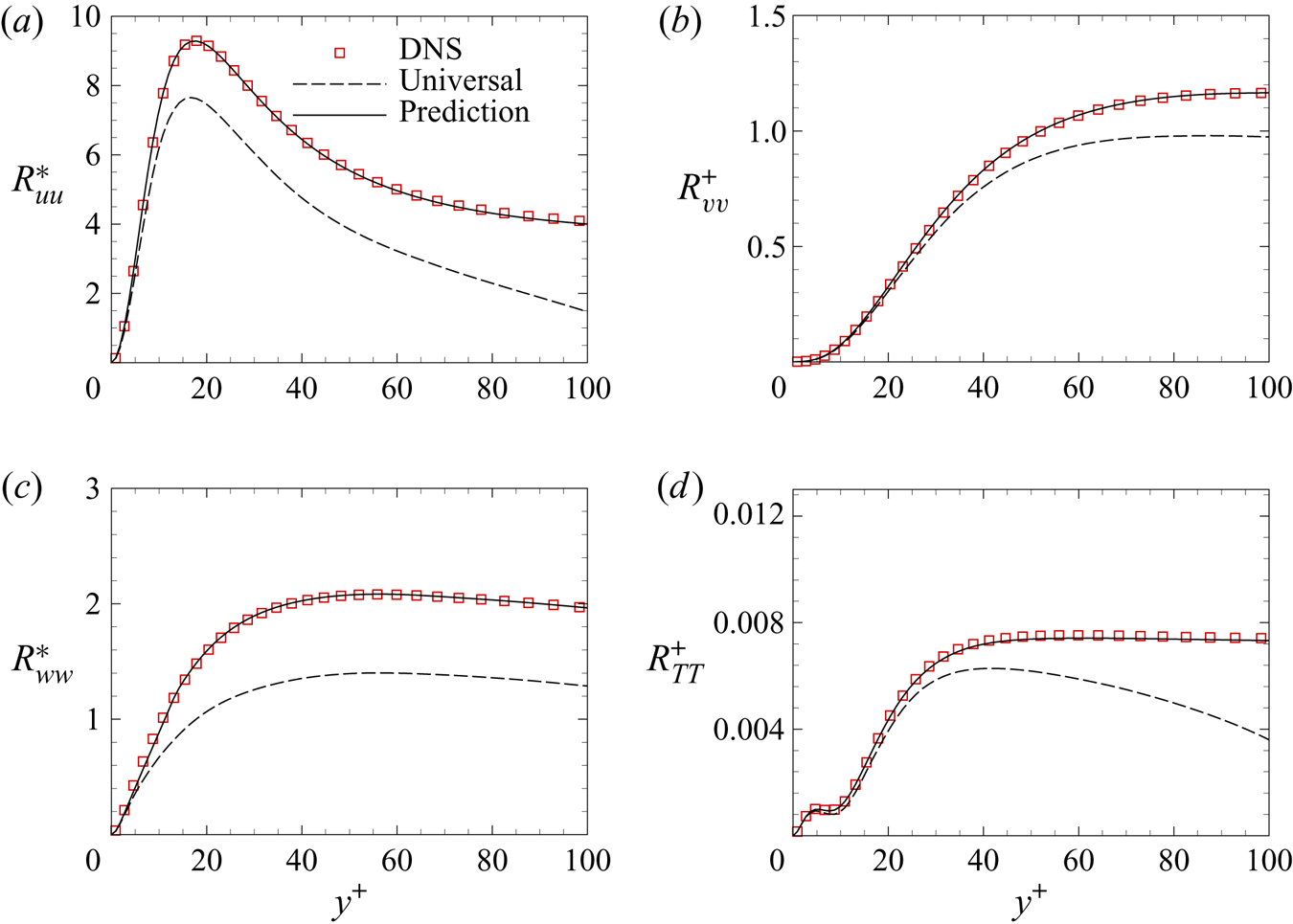
The variances of the predicted near-wall fluctuations are shown in figure 15, along with the results of DNS and universal signals. Compared with the DNS results, the variances of the universal signals are much lower due to the absence of the large-scale signal. This discrepancy is remedied by incorporating the large-scale motions in the predictive model (Yin et al. Reference Yin, Huang and Xu2018). Henceforth, the variances of the predicted results agree well with the DNS results.
Predicted fluctuation variances normalized by viscous scales, (a)  $R^*_{uu}$, (b)
 $R^*_{vv}$, (c)
 $R^*_{ww}$, (d)
 $R^+_{TT}$, compared with DNS results and universal signals.

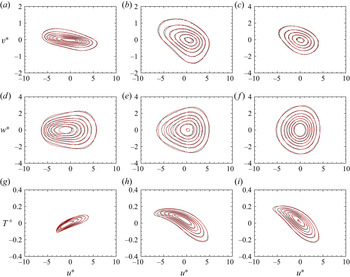
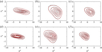
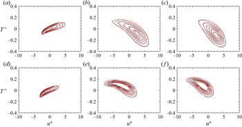
We further compare the joint p.d.f. distributions of the predicted results with the DNS data, as presented in figure 16. The results at three different wall-normal locations  $y^+=15$, 30 and 50 for
 $P(u^*,v^*)$ and
 $P(u^*,w^*)$ and
 $y^+=5$, 30 and 50 for
 $P(u^*,T^+)$ are presented. The predicted joint p.d.f.s agree reasonably well with the DNS results, validating the presently proposed predictive models. Notably, the prediction for temperature fluctuations at
 $y^+=15$ is not so successful. This is because the mean temperature gradient is nearly zero at this location, where the correlation between velocity and temperature goes through intense variation from positive to negative, as has been shown in figure 8. The correlation coefficients in the large-scale high- and low-speed regions are very different. This requires further refinements of the predictive model, which will be considered in our future study.
Joint p.d.f. distributions, (a–c)  $P(u^*,v^*)$, (d–f)
 $P(u^*,w^*)$, (g–i)
 $P(u^*,T^+)$, (a,d) at
 $y^+=15$, (g) at
 $y^+=5$, (b,e,h) at
 $y^+\!=\!30$, (c, f,i) at
 $y^+\!=\!50$. Black lines, DNS; red lines, predicted.

Lastly, in order to further verify whether the modulation effects are correctly predicted, we present the joint p.d.f. distributions within large-scale high- and low-speed regions. The results are displayed in figures 17–19. The predicted joint p.d.f. distributions collapse well with the DNS results in both the large-scale high- and low-speed regions, indicating the modulation effects and the splatting-induced distortions are both accurately represented in the prediction. Specifically, the joint p.d.f.s  $P(u^*,w^*)$ in the region of
 $u''_L > u_t$ are well-described, where the spanwise velocity component are widely distributed due to the strong dispersive motion (Hwang et al. Reference Hwang, Lee, Sung and Zaki2016; Yin et al. Reference Yin, Huang and Xu2018). Moreover, although the inclination angles of the ‘tear-drop’ shaped joint p.d.f.s
 $P(u^*,T^+)$ at
 $y^+=30$ and
 $y^+=50$ within the large-scale high- and low-speed regions differ greatly, they can still be accurately predicted.
Joint p.d.f.s  $P(u^*,v^*)$ in the region of (a–c)
 $u''_L > u_t$ and (d–f)
 $u''_L < -u_t$ at (a,d)
 $y^+=15$, (b,e)
 $y^+=30$ and (c, f)
 $y^+=50$. Black lines, DNS; red lines, predicted.

7. Concluding remarks
In the present study, we proposed a predictive model for the near-wall turbulent fluctuations in compressible wall turbulence. In this model, the predicted velocity is expressed as the summation of the modulated small-scale signals by the large-scale streamwise velocity and the imprints of outer-region large-scale signal on the near-wall region, where the mean density variation is involved to alleviate the possible Mach number dependence of the statistics. The predictive model for temperature is derived based on the modified SRA proposed by Gaviglio (Reference Gaviglio1987) (the GSRA), and the predictive model for velocity. The obtained formula manifests that the predictive model should also be written as the summation of the small- and large-scale signals, where the small-scale temperature is modulated by the large-scale streamwise velocity as a quadratic function. The large-scale streamwise velocity component and temperature in the near-wall region is obtained by the spectral linear stochastic estimation, while the other two velocity components by linear mapping. The modulation on the upper and lower envelopes is considered separately for the streamwise velocity and temperature fluctuations to incorporate the splatting-induced distortion, although this effect is insignificant above  $y^+=30$. The modulation coefficients are obtained by the newly proposed approximate algebraic method without iterative procedures, which is further validated to give accurate results. The phase shift between the modulation and superposition is also considered. The extracted universal signals from the raw DNS data is proved to be free from the influence of the LSMs, indicating its validity.
A DNS database for compressible channel flow at  $Re_\tau = 1170$ and
 $M_b=2.89$ is established and validated, based on which direct observations and quantitative descriptions of superposition and modulation effects of the LSMs in the outer region on the near-wall small-scale turbulent fluctuations are presented, and the validation of the predictive models are discussed. The fluctuation variances and joint p.d.f. distribution of the predicted fluctuations agree well with those of the DNS data, proving the validity of the presently proposed predictive model.
Although the present predictive model is calibrated and validated at only one Mach number, we believe it to be applicable to other Mach number flows with adiabatic or quasi-adiabatic walls as well. On one hand, the density-weighted velocity fluctuations are nearly identical for the same  $Re_\tau$, for the genuine compressibility effects induced by dilatational motions are negligible in compressible turbulent channel flows, as we have proved in our previous studies (Yu et al. Reference Yu, Xu and Pirozzoli2019). On the other hand, since the fluctuation intensities of temperature and the streamwise velocity are related by the SRA, its application to other Mach numbers is promising. A direct validation will be duly taken into consideration in our future study.
The possible limitations of the presently proposed predictive models lie in the following aspects. First, the universality of the calibrated parameters against the Reynolds number is left untested. This will be considered in our further study when the databases at higher Reynolds numbers are available. Second, for other thermal boundary conditions, especially on cold walls, the turbulent structures are highly modulated by the mean property gradients near the wall (Duan, Beekman & Martin Reference Duan, Beekman and Martin2010; Patel, Boersma & Pecnik Reference Patel, Boersma and Pecnik2016), the near-wall turbulence may not be as universal as in incompressible turbulence. Third, it is still challenging to provide accurate temperature fluctuations near the local maximum of the mean temperature due to the invalidity of the SRA (Zhang et al. Reference Zhang, Bi, Hussain and She2014). These aspects will be considered in our future study.
Joint p.d.f.s  $P(u^*,w^*)$ under the condition of (a–c)
 $u''_L > u_t$ and (d–f)
 $u''_L < -u_t$ at (a,d)
 $y^+=15$, (b,e)
 $y^+=30$ and (c, f)
 $y^+=50$. Black lines, DNS; red lines, predicted.

Joint p.d.f.s  $P(u^*,T^+)$ under the condition of (a–c)
 $u''_L > u_t$ and (d–f)
 $u''_L < -u_t$ at (a,d)
 $y^+=5$, (b,e)
 $y^+=30$ and (c, f)
 $y^+=50$. Black lines, DNS; red lines, predicted.

Funding
This work was supported by the Open Project of State Key Lab of Aerodynamics (grant no. SKLA-20200102) and the National Natural Science Foundation of China (grant no. 91752205).
Declaration of interests
The authors report no conflict of interest.
Appendix. Mach number independence of density-weighted velocity fluctuation variances
This appendix serves as supplementary proof for Mach number independence of density-weighted velocity fluctuation variances. This is the essence of Morkovin's hypothesis (Morkovin Reference Morkovin1962), and has been validated widely by previous studies (Duan Reference Duan2011; Yu et al. Reference Yu, Xu and Pirozzoli2019). Herein, we further prove that the large-scale and small-scale fluctuation variances both satisfy this conclusion.
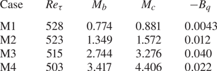
We adopt the database in our previous study at  $Re_\tau \approx 500$ (Yu et al. Reference Yu, Xu and Pirozzoli2019). The flow parameters are listed in table 2. The lengths of the computational domain in the streamwise and spanwise directions are
 $2{\rm \pi} h$ and
 ${\rm \pi} h$. The scale for separating the large- and small-scale motions are
 $\lambda _x = 2.0h$ and
 $\lambda _z =0.5 h$, respectively.
Flow parameters for cases in Yu et al. (Reference Yu, Xu and Pirozzoli2019). Here  $Re_{\tau }$ is the friction Reynolds number,
 $M_b$ and
 $M_c$ are the bulk and centreline Mach number and
 $-B_q=T_{\tau }/T_w$ is the heat flux parameter.

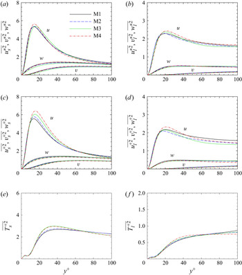
The variances for velocity fluctuations with and without being density weighted are displayed in figure 20(a–d). It is obvious that after being weighted by density, both the large- and small-scale fluctuation variances show weak Mach number dependence, while those not weighted by density do not show this characteristic. We also present in figure 20(e–f) the temperature fluctuation variances, which are Mach number independent under the parameter settings in the present study. Similarly, the spectra and joint p.d.f.s of the density-weighted velocity have been compared, showing similar consistency. These results are omitted here for brevity.
Variances of velocity fluctuation (a,b) density-weighted, (c,d) not weighted by density. (e–f) Temperature fluctuation variances. (a,c,e) Small-scale portion, (b,d, f) large-scale portion.