1 Introduction
When an upstream vortical field impinges on a solid body its normal velocity component is abruptly forced to zero due to a no-penetration condition. This results in the generation of pressure fluctuation on the surface, which in the case of an aerofoil, radiate as a dipole sound primarily from the aerofoil leading edge (LE). Accordingly this noise mechanism is usually referred to as LE noise or aerofoil–turbulence interaction (ATI) noise, and is often considered to be one of the major noise sources, particularly in the presence of significant upstream disturbances (Migliore & Oerlemans Reference Migliore and Oerlemans2004). Such conditions are regularly met in a variety of engineering applications, for example contra-rotating fans, propellers, turbofan outlet-guide vanes, high-lift devices and wind farms. Over the years many approaches have been adopted for the study of ATI noise to understand both the physical noise generation mechanisms and the influence of various geometric parameters such as aerofoil thickness, angle of attack and camber. This includes the theoretical model of Amiet (Reference Amiet1975) and its subsequent extensions, namely, the convection of two-dimensional frozen turbulence in a uniform mean flow (Roger & Moreau Reference Roger and Moreau2010); theoretical and numerical approaches based on harmonic gusts (Goldstein Reference Goldstein1978; Atassi, Subramaniam & Scott Reference Atassi, Subramaniam and Scott1990; Myers & Kerschen Reference Myers and Kerschen1995, Reference Myers and Kerschen1997; Lockard & Morris Reference Lockard and Morris1998; Evers & Peake Reference Evers and Peake2000; Ayton & Peake Reference Ayton and Peake2013, Reference Ayton and Peake2015; Gill, Zhang & Joseph Reference Gill, Zhang and Joseph2013); experimental approaches based on grid-generated homogeneous isotropic turbulence (Paterson & Amiet Reference Paterson and Amiet1976; Moreau, Roger & Jurdic Reference Moreau, Roger and Jurdic2005; Devenport, Staubs & Glegg Reference Devenport, Staubs and Glegg2010); and recent computational approaches based on two- or three-dimensional Euler and Navier–Stokes simulations (Christophe et al. Reference Christophe, Anthoine, Rambaud, Schram, Mathey and Moreau2007; Christophe, Anthoine & Rambaud Reference Christophe, Anthoine and Rambaud2008; Deniau et al. Reference Deniau, Boussuge, Polacsek and Moreau2011; Gill, Zhang & Joseph Reference Gill, Zhang and Joseph2015; Kim & Haeri Reference Kim and Haeri2015).
Research conducted in the previous a few years has shown that a potential passive treatment capable of large reductions to ATI noise is the inclusion of an undulated (wavy) aerofoil leading edge. Such a geometry was originally considered for its aerodynamic properties (Miklosovic et al.
Reference Miklosovic, Murray, Howle and Fish2004; Johari et al.
Reference Johari, Henoch, Custodio and Levshin2007; Hansen, Kelso & Dally Reference Hansen, Kelso and Dally2011; Hansen et al.
Reference Hansen, Rostamzadeh, Kelso and Dally2016), and is inspired by the leading-edge protrusions (tubercles) of the humpback whale’s pectoral flippers, thought to be responsible for its impressive manoeuvrability when catching its prey (Fish, Howle & Murray Reference Fish, Howle and Murray2008). One of the first attempts to quantify the aeroacoustic properties of wavy leading edges (WLEs) was conducted by Hansen, Kelso & Doolan (Reference Hansen, Kelso and Doolan2012), who through experiments based on a NACA0021 aerofoil identified that WLE cases obtained large tonal and broadband self-noise reductions within a certain frequency range. They theorised that the noise reductions were related to the production of streamwise vortices at the leading-edge troughs, which enhance the stability of the boundary layer by mixing in higher momentum fluid from the free stream, altering the generation of vorticity near the trailing edge. In the meantime, a large effort has been made towards quantifying the extent of ATI noise reductions based on various geometric parameters, particularly the WLE amplitude (
 $h_{LE}$
) and wavelength (
 $\unicode[STIX]{x1D706}_{LE}$
) (Clair et al.
Reference Clair, Polacsek, Garrec, Reboul, Gruber and Joseph2013; Lau, Haeri & Kim Reference Lau, Haeri and Kim2013; Chaitanya et al.
Reference Chaitanya, Narayanan, Joseph, Vanderwel, Turner, Kim and Gantapathisubramani2015; Narayanan et al.
Reference Narayanan, Chaitanya, Haeri, Joseph, Kim and Polacsek2015; Kim, Haeri & Joseph Reference Kim, Haeri and Joseph2016). It is consistently found that the level of noise reduction is positively influenced by increasing
 $h_{LE}$
. Comparatively, altering
 $\unicode[STIX]{x1D706}_{LE}$
seems to have a smaller effect.
Narayanan et al. (Reference Narayanan, Chaitanya, Haeri, Joseph, Kim and Polacsek2015) performed an experimental parametric study based on grid-generated homogeneous isotropic turbulence and noted that more noise reductions were achievable for lower flow speeds (
 $U_{\infty }$
) and thinner aerofoils. One of their most significant findings was a consistent starting frequency of noise reduction:
 $f_{0}=\unicode[STIX]{x1D6FC}U_{\infty }/(2h_{LE})$
, where
 $\unicode[STIX]{x1D6FC}\approx 0.5$
for all cases. This finding is also supported by the work of Clair et al. (Reference Clair, Polacsek, Garrec, Reboul, Gruber and Joseph2013) who observed a broader frequency range of noise reduction for a reduced flow speed. A further parametric study was conducted by Chaitanya et al. (Reference Chaitanya, Narayanan, Joseph, Vanderwel, Turner, Kim and Gantapathisubramani2015) focusing on the WLE serration angle defined as
 $\unicode[STIX]{x1D703}=\tan ^{-1}(4h_{LE}/\unicode[STIX]{x1D706}_{LE})$
. They concluded that, for a given WLE amplitude and turbulence integral length scale, there exists an optimum serration angle for maximum noise reduction. This means that increasing
 $\unicode[STIX]{x1D706}_{LE}$
can result in either an increase or decrease of noise reduction depending on whether
 $\unicode[STIX]{x1D703}$
is higher than the optimal value or lower, which explains some inconsistent observations (on the effect of
 $\unicode[STIX]{x1D706}_{LE}$
) made between Lau et al. (Reference Lau, Haeri and Kim2013) and Narayanan et al. (Reference Narayanan, Chaitanya, Haeri, Joseph, Kim and Polacsek2015). Chaitanya et al. (Reference Chaitanya, Narayanan, Joseph, Vanderwel, Turner, Kim and Gantapathisubramani2015) also showed that the noise reduction increases with frequency as a power law. Meanwhile, an analytical study by Mathews & Peake (Reference Mathews and Peake2015) suggested that there exist noise-increasing eddy components in the impinging turbulence depending on their orientation relative to the leading edge. It is, however, speculated that the probability of such eddies is lower in the WLE cases and the averaged effect yields a consistent noise reduction.
Despite rapid growth in the field, the understanding of the noise reduction mechanisms associated with WLEs is still underdeveloped. A significant progress has recently been made by Kim et al. (Reference Kim, Haeri and Joseph2016) who carried out high-fidelity numerical simulations based on three-dimensional nonlinear compressible Euler equations and synthetic inflow turbulence (Kim & Haeri Reference Kim and Haeri2015). They identified two primary noise reduction mechanisms: a source cutoff effect and a phase interference effect. The source cutoff effect was recognised by analysing the auto-spectrum of the fluctuating wall pressure at different points along the WLE, revealing a substantial reduction in source strength at the hill region across the whole frequency range. It was suggested that this was due to the geometric obliqueness relative to the incoming flow turbulence. Arguably more intriguing is that significant source strength differences were observed between the peak and root, despite the fact that both has zero obliqueness against the incoming disturbances similar to a straight leading-edge (SLE) case. At low frequencies, the peak exhibited a substantially lower source strength than the root, while at high frequencies, the peak seemed to overtake the root by a small margin. Overall, the source strength at the root was comparable to that of the SLE at all frequencies. Regarding the phase interference effect, it was reported that the two-point phase spectra between the peak and other points along the WLE experiences an increased level of phase shifts towards
 $\unicode[STIX]{x03C0}$
(out of phase) compared to the SLE case.
Guided by the earlier findings, the present work is aimed to extend the understanding of the aeroacoustic source mechanisms associated with the WLEs interacting with vortical disturbances. Here we focus on explaining the disparity in source characteristics between the peak and root as outlined above. The current study is based on a computational approach similar to Kim & Haeri (Reference Kim and Haeri2015), Kim et al. (Reference Kim, Haeri and Joseph2016) except that a single spanwise vortex model is used instead of synthetic inflow turbulence to create vortical disturbances. Using the single vortex model has two main advantages over the synthetic turbulence approach. First, it offers enhanced clarity in observing and identifying major physical phenomena taking place during the aerofoil–vortex interaction process. Secondly, there still is a reasonable range of frequency components in the vortical disturbances, unlike harmonic gust approaches, and the resulting spectra are much cleaner than those from the synthetic turbulence approach.
The current simulation result shows that the prescribed vortex impinging on the aerofoil creates secondary vortices along the WLE which form a horseshoe-like vortex system which tends to intensify as time elapses. The three-dimensional dynamics of the horseshoe vortex system is carefully investigated with regard to the induced velocity field around the WLE, from which the wall pressure fluctuation (aeroacoustic source strength) is deduced. The problem is also modelled semi-analytically by using Biot–Savart’s law to further support the hypothesis proposed in the current study. It should be noted that the current study is still based on a zero-thickness aerofoil in an inviscid flow at zero mean incidence angle and low Mach number. It is expected that a realistic aerofoil (with a thickness and/or camber) and a non-uniform viscous mean flow may develop increasingly complex mechanisms associated with self-generated leading-edge vortices (Hansen et al. Reference Hansen, Rostamzadeh, Kelso and Dally2016) and viscous distortion/dissipation of the vortices. Prior to the additional complexity to be investigated, the current study focuses on the most basic form of the aerofoil–vortex interaction and therefore the simplest geometry and flow condition are chosen in this paper.
This paper is structured and written in the following order. Section 2 introduces the computational set-up and methods used in this study, including details of the prescribed spanwise vortex model implemented in the current simulations. Section 3 provides initial observations obtained from the simulations including wall and far-field pressure spectra for various WLE geometries. Additionally, it includes a qualitative discussion of the secondary vortex structures created along the WLE and how they influence the induced velocity field. Section 4 provides quantitative explanations as to how the aeroacoustic source strength at the root region is maintained at a level similar to the SLE case. Section 5 moves the focus on to the peak region and explain the trend of the source strength decaying (but converging) with the WLE amplitude, which is also supported by the semi-analytic model derived from Biot–Savart’s law. In § 6 supplementary observations are made with respect to a similarity rule in the source strength and the effect of three-dimensionality in the impinging vortex. Finally concluding remarks are provided in § 7.
2 Description of the problem and computational set-up
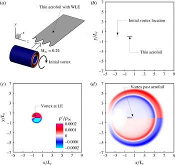
The current problem of aerofoil noise generation due to interaction with a prescribed spanwise vortex impinging on the leading edge is illustrated in figure 1. Instantaneous snapshots of the computed pressure field exhibit sound waves generated and radiated during and after the interaction. This section describes the problem set-up and the computational methodologies used in this study.
2.1 Computational domain and aerofoil geometry
The computational domain in a rectangular cuboid contains a flat-plate aerofoil at the centre with zero thickness and zero angle of attack. The zero-thickness aerofoil is modelled by using a H-topology grid system where the central branch section represents the aerofoil’s upper and lower surfaces with no gap between them. The longitudinal and vertical boundaries of the domain are surrounded by a sponge layer through which the flow is (gently) forced to maintain the potential mean flow condition. Any acoustic waves are attenuated and absorbed in the sponge layer to prevent numerical reflections at the outer boundaries. The lateral boundaries of the domain are interconnected via a periodic boundary condition. The entire computational domain; the inner region (physical domain) where meaningful simulation data are obtained; and, the sponge layer zone are defined as
 $$\begin{eqnarray}\displaystyle \left.\begin{array}{@{}c@{}}\displaystyle {\mathcal{D}}_{\infty }=\{\boldsymbol{x}\mid x/L_{c}\in [-5,9],\quad y/L_{c}\in [-7,7],\quad z\in [-{\textstyle \frac{1}{2}}L_{z},{\textstyle \frac{1}{2}}L_{z}]\},\\ \displaystyle {\mathcal{D}}_{physical}=\{\boldsymbol{x}\mid x/L_{c}\in [-3,3],\quad y/L_{c}\in [-5,5],\quad z\in [-{\textstyle \frac{1}{2}}L_{z},{\textstyle \frac{1}{2}}L_{z}]\},\\ \displaystyle {\mathcal{D}}_{sponge}={\mathcal{D}}_{\infty }-{\mathcal{D}}_{physical},\end{array}\right\} & & \displaystyle\end{eqnarray}$$
where
 $L_{c}$
denotes the mean chord length of the aerofoil and
 $L_{z}$
is the spanwise length of the domain. The origin of the domain is located at the centre of the aerofoil surface. In the current simulations,
 $L_{z}$
is set to cover one wavelength of the WLE profile given. The free-stream Mach number is set to
 $M_{\infty }=u_{\infty }/a_{\infty }=0.24$
. This Mach number is the same as used in the previous work by Kim et al. (Reference Kim, Haeri and Joseph2016).
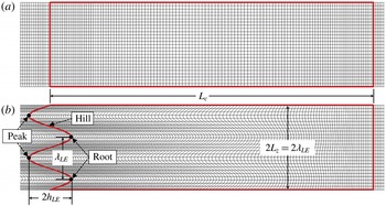
The aerofoil has a WLE (wavy leading edge) which is profiled by using a sine function where the most protruded points are defined as ‘peak’, the least as ‘root’ and the middle as ‘hill’ as denoted in figure 2. Herein,
 $h_{LE}$
is the WLE amplitude (
 $2h_{LE}$
being the peak-to-root amplitude) and
 $\unicode[STIX]{x1D706}_{LE}$
is the spanwise wavelength of the WLE. The WLE profile in this study is defined by
 $$\begin{eqnarray}\displaystyle x_{LE}(z)=-\frac{1}{2}L_{c}+h_{LE}\sin \left(\frac{2\unicode[STIX]{x03C0}z}{\unicode[STIX]{x1D706}_{LE}}\right),\quad z\in \left[-\frac{1}{2}L_{z},\frac{1}{2}L_{z}\right], & & \displaystyle\end{eqnarray}$$
where the location of the trailing edge is fixed at
 $x_{TE}=L_{c}/2$
. The spanwise coordinates of the peak, hill centre and root are
 $z=-\unicode[STIX]{x1D706}_{LE}/4$
, 0 and
 $\unicode[STIX]{x1D706}_{LE}/4$
, respectively. The default wavelength of the WLE in the current study is
 $\unicode[STIX]{x1D706}_{LE}/L_{c}=2/15$
and in § 6
 $\unicode[STIX]{x1D706}_{LE}/L_{c}=4/15$
is used as well. The baseline WLE amplitude is
 $h_{LE}/L_{c}=1/15$
and lower/higher values of
 $h_{LE}$
are also explored to investigate the effect of
 $h_{LE}$
. These geometric parameters are similar to those used in Kim et al. (Reference Kim, Haeri and Joseph2016).
Description of the current problem: a prescribed spanwise vortex impinging on a thin aerofoil with a wavy leading edge: (a) schematic diagram, (b) initial condition, (c) during the interaction and (d) after the interaction. The mean aerofoil chord is denoted by
 $L_{c}$
.

Surface meshes (coarsened for illustration purposes) on the flat-plate aerofoils used in the present study, with (a) straight and (b) wavy leading edges (SLE and WLE, respectively). The case of
 $h_{LE}/L_{c}=1/15$
and
 $\unicode[STIX]{x1D706}_{LE}/L_{c}=2/15$
is shown in this figure.

2.2 Governing equations and numerical methods
Aerofoil noise generated by interaction with vortical disturbances is largely considered an inviscid phenomenon and therefore exclusion of viscous terms is usually considered to be a reasonable simplification (Goldstein Reference Goldstein1978; Atassi et al. Reference Atassi, Subramaniam and Scott1990; Myers & Kerschen Reference Myers and Kerschen1995; Lockard & Morris Reference Lockard and Morris1998; Evers & Peake Reference Evers and Peake2000; Ayton & Peake Reference Ayton and Peake2013; Gill et al. Reference Gill, Zhang and Joseph2015; Kim & Haeri Reference Kim and Haeri2015). Following up on the historical approach, we employ full three-dimensional (3-D) compressible Euler equations (with a source term for the sponge layer mentioned earlier) in a conservative form transformed onto a generalised coordinate system:
 $$\begin{eqnarray}\displaystyle \frac{\unicode[STIX]{x2202}}{\unicode[STIX]{x2202}t}\left(\frac{\boldsymbol{Q}}{J}\right)+\frac{\unicode[STIX]{x2202}}{\unicode[STIX]{x2202}\unicode[STIX]{x1D709}_{i}}\left(\frac{\boldsymbol{F}_{j}}{J}\frac{\unicode[STIX]{x2202}\unicode[STIX]{x1D709}_{i}}{\unicode[STIX]{x2202}x_{j}}\right)=-\frac{a_{\infty }}{L_{c}}\frac{\boldsymbol{S}}{J}, & & \displaystyle\end{eqnarray}$$
where
 $i=1,2,3$
; and,
 $j=1,2,3$
denote the three dimensions. In (2.3), the conservative variable and flux vectors are given by
 $$\begin{eqnarray}\displaystyle \left.\begin{array}{@{}c@{}}\displaystyle \boldsymbol{Q}=[\unicode[STIX]{x1D70C},\unicode[STIX]{x1D70C}u,\unicode[STIX]{x1D70C}v,\unicode[STIX]{x1D70C}w,\unicode[STIX]{x1D70C}e_{t}]^{\text{T}},\\ \displaystyle \boldsymbol{F}_{j}=[\unicode[STIX]{x1D70C}u_{j},(\unicode[STIX]{x1D70C}uu_{j}+\unicode[STIX]{x1D6FF}_{1j}p),(\unicode[STIX]{x1D70C}vu_{j}+\unicode[STIX]{x1D6FF}_{2j}p),(\unicode[STIX]{x1D70C}wu_{j}+\unicode[STIX]{x1D6FF}_{3j}p),(\unicode[STIX]{x1D70C}e_{t}+p)u_{j}]^{\text{T}},\end{array}\right\} & & \displaystyle\end{eqnarray}$$
where
 $\unicode[STIX]{x1D709}_{i}=\{\unicode[STIX]{x1D709},\unicode[STIX]{x1D702},\unicode[STIX]{x1D701}\}$
are the generalised coordinates,
 $x_{j}=\{x,y,z\}$
are the Cartesian coordinates,
 $u_{j}=\{u,v,w\}$
,
 $e_{t}=p/[(\unicode[STIX]{x1D6FE}-1)\unicode[STIX]{x1D70C}]+u_{j}u_{j}/2$
and
 $\unicode[STIX]{x1D6FE}=1.4$
for air. In the current set-up,
 $\unicode[STIX]{x1D709}$
,
 $\unicode[STIX]{x1D702}$
and
 $\unicode[STIX]{x1D701}$
are body fitted coordinates along the grid lines in the streamwise, vertical and lateral directions, respectively. The Jacobian determinant of the coordinate transformation (from Cartesian to the body fitted) is given by
 $J^{-1}=|\unicode[STIX]{x2202}(x,y,z)/\unicode[STIX]{x2202}(\unicode[STIX]{x1D709},\unicode[STIX]{x1D702},\unicode[STIX]{x1D701})|$
(Kim & Morris Reference Kim and Morris2002). The extra source term
 $\boldsymbol{S}$
on the right-hand side of (2.3) is non-zero within the sponge layer only, which is described in Kim, Lau & Sandham (Reference Kim, Lau and Sandham2010).
In this work, the governing equations given above are solved by using high-order accurate numerical methods specifically developed for aeroacoustic simulations on structured grids. The flux derivatives in space are calculated based on fourth-order pentadiagonal compact finite difference schemes with seven-point stencils (Kim Reference Kim2007). Explicit time advancing of the numerical solution is carried out by using the classical fourth-order Runge–Kutta scheme with the CFL (Courant–Friedrichs–Lewy) number of 0.95. Numerical stability is maintained by implementing sixth-order pentadiagonal compact filters for which the cutoff wavenumber (normalised by the grid spacing) is set to
 $0.85\unicode[STIX]{x03C0}$
(Kim Reference Kim2010). In addition to the sponge layers used, characteristics-based non-reflecting boundary conditions (Kim & Lee Reference Kim and Lee2000) are applied at the far boundaries in order to prevent any outgoing waves from returning to the computational domain. Periodic conditions are used across the spanwise boundary planes as indicated earlier. Slip wall (no-penetration) boundary conditions are implemented on the aerofoil surface (Kim & Lee Reference Kim and Lee2004) and also on the centre plane downstream of the aerofoil. The latter is intended to eliminate the secondary interaction which takes place at the trailing edge, and therefore to focus on the leading-edge interaction only.
The simulation is carried out on a total of 43 760 640 grid cells (
 $1036\times 660\times 64$
) where the smallest cells are located at the aerofoil LE with the size of
 $\unicode[STIX]{x0394}x=\unicode[STIX]{x0394}y=0.00625L_{c}$
and
 $\unicode[STIX]{x0394}z=0.002083L_{c}$
. Although the grid is gradually stretched outwards, a high grid resolution is still maintained in the far field in order to capture the high-frequency components radiated. At least 46 cells are located across the diameter of the initial vortex. The computation is parallelised via domain decomposition and message passing interface (MPI) approaches. The compact finite difference schemes and filters used are implicit in space due to the inversion of pentadiagonal matrices involved, which requires a precise and efficient technique for the parallelisation in order to avoid numerical artefacts that may appear at the subdomain boundaries. A recent parallelisation approach based on quasi-disjoint matrix systems (Kim Reference Kim2013) offering super-linear scalability is used in the present paper. The entire domain is decomposed and distributed onto 480 separate computing nodes/subdomains (
 $20\times 12\times 2$
in the streamwise, vertical and spanwise directions, respectively). A grid convergence test has been performed for the current computational set-up – see appendix A.
2.3 Prescribed spanwise vortex model
The spanwise (two-dimensional) vortex model prescribed as an initial condition in this study is based on the Gaussian synthetic eddy profile used in previous publications (Kim & Haeri Reference Kim and Haeri2015; Kim et al.
Reference Kim, Haeri and Joseph2016). It provides a divergence-free velocity field via taking the curl of the following vector potential, i.e.
 $\boldsymbol{u}^{\prime }(\boldsymbol{x},t=0)=\unicode[STIX]{x1D735}\times [\unicode[STIX]{x1D6F9}(\boldsymbol{x})\boldsymbol{e}_{z}]$
:
 $$\begin{eqnarray}\displaystyle \unicode[STIX]{x1D6F9}(\boldsymbol{x})=a_{\infty }L_{c}\frac{\unicode[STIX]{x1D716}}{\sqrt{\unicode[STIX]{x1D70E}}}\exp \{-[3\unicode[STIX]{x1D70E}r(\boldsymbol{x})]^{2}\},\quad r(\boldsymbol{x})=\frac{(x-x_{0})^{2}+y^{2}}{L_{c}^{2}}, & & \displaystyle\end{eqnarray}$$
where
 $\unicode[STIX]{x1D716}$
and
 $\unicode[STIX]{x1D70E}$
are control parameters for the vortex strength and size, respectively;
 $x_{0}=-2.5L_{c}$
is the streamwise coordinate of the starting point of the vortex core; and,
 $\boldsymbol{e}_{z}$
is a Cartesian unit vector in the spanwise direction. This results in the following formulae for the velocity field at
 $t=0$
:
 $$\begin{eqnarray}\displaystyle u(\boldsymbol{x})=u_{\infty }-36\frac{\unicode[STIX]{x1D70E}^{2}}{L_{c}^{2}}yr(\boldsymbol{x})\unicode[STIX]{x1D6F9}(\boldsymbol{x}),\quad v(\boldsymbol{x})=36\frac{\unicode[STIX]{x1D70E}^{2}}{L_{c}^{2}}(x-x_{0})r(\boldsymbol{x})\unicode[STIX]{x1D6F9}(\boldsymbol{x}), & & \displaystyle\end{eqnarray}$$
while the pressure and the density are set to ambient/quiescent conditions (
 $p_{\infty }$
and
 $\unicode[STIX]{x1D70C}_{\infty }$
). The control parameters are set to
 $\unicode[STIX]{x1D716}=-0.00228$
and
 $\unicode[STIX]{x1D70E}=14.4$
such that the level and the length scale of the velocity perturbation (
 $0.025u_{\infty }$
and
 $0.1L_{c}$
, respectively) are similar to those of the large eddies used in the previous experiments by Narayanan et al. (Reference Narayanan, Chaitanya, Haeri, Joseph, Kim and Polacsek2015) and Chaitanya et al. (Reference Chaitanya, Narayanan, Joseph, Vanderwel, Turner, Kim and Gantapathisubramani2015). The parameters were determined via the following definition of perturbation length scale in this paper:
 $$\begin{eqnarray}\displaystyle \text{perturbation-length-scale}=\frac{1}{\max |v(x)|}\int _{x_{0}}^{x_{0}+\infty }|v(x)|\,\text{d}x\quad \text{at }y=z=t=0. & & \displaystyle\end{eqnarray}$$
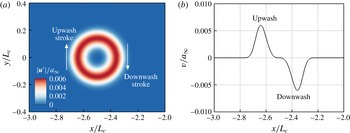
The resulting velocity field is plotted in figure 3. The prescribed vortex induces clockwise rotating velocity components, firstly making a downwash stroke on to the aerofoil leading edge followed by an upwash stroke as the vortex travels further downstream. It is shown in figure 1 that the downwash–upwash strokes create compression–expansion pressure waves on the upper side of the leading edge radiating towards the top (with the opposite taking place on the lower side).
The initial velocity field induced by the spanwise vortex model given by (2.6): (a) induced velocity magnitude contours and (b) the vertical velocity profile along the centreline (
 $y=0$
).

3 Initial findings and the questions emerged
The simulations are run until a non-dimensional time of
 $ta_{\infty }/L_{c}=20$
, which is sufficient to capture both the fluctuating wall pressure signals and the far-field sound. For the subsequent sections, the following quantities are used repeatedly. Fluctuating acoustic and wall pressures are denoted by
 $p_{a}^{\prime }$
and
 $\unicode[STIX]{x0394}p_{w}$
, respectively, defined here as
 $$\begin{eqnarray}\displaystyle p_{a}^{\prime }(\boldsymbol{x},t)=p_{a}(\boldsymbol{x},t)-p_{\infty },\quad \unicode[STIX]{x0394}p_{w}(\boldsymbol{x},t)=p_{w}(x,y=0^{+},z,t)-p_{w}(x,y=0^{-},z,t),\quad \qquad & & \displaystyle\end{eqnarray}$$
where the subscripts
 $y=0^{+}$
and
 $0^{-}$
indicate the upper and lower surfaces of the flat-plate aerofoil, respectively. The wall pressure fluctuation (
 $\unicode[STIX]{x0394}p_{w}$
) defined in this paper is therefore representing the aeroacoustic source strength. The power spectral density (PSD) of the wall pressure fluctuation can then be determined as
 $$\begin{eqnarray}\displaystyle S_{ppw}(\boldsymbol{x},f)=2\widehat{\unicode[STIX]{x0394}p_{w}}(\boldsymbol{x},f)\widehat{\unicode[STIX]{x0394}p_{w}}^{\ast }(\boldsymbol{x},f), & & \displaystyle\end{eqnarray}$$
where ‘
 $\wedge$
’ represents a Fourier transformed variable and ‘
 $\ast$
’ denotes a complex conjugate. For the subsequent analysis surface quantities are extracted one grid point aft of the leading edge, where the largest pressure fluctuation is obtained in the current simulations. Similarly the PSD of the acoustic pressure may be determined as
 $$\begin{eqnarray}\displaystyle S_{ppa}(\boldsymbol{x},f)=2\widehat{p_{a}^{\prime }}(\boldsymbol{x},f)\widehat{p_{a}^{\prime }}^{\ast }(\boldsymbol{x},f), & & \displaystyle\end{eqnarray}$$
which is calculated at an observer location
 $\boldsymbol{x}_{o}=(0,5L_{c},0)$
in the present study. The sound attenuation due to a WLE relative to the SLE case is then quantified by
 $$\begin{eqnarray}\displaystyle \unicode[STIX]{x0394}\text{SPL}(\boldsymbol{x},f)=10\log _{10}\left[\frac{S_{ppa}(\boldsymbol{x},f)|_{SLE}}{S_{ppa}(\boldsymbol{x},f)|_{WLE}}\right]. & & \displaystyle\end{eqnarray}$$
Fluctuating wall pressure time signals,
 $\unicode[STIX]{x0394}p_{w}(t^{\ast })/p_{\infty }$
, and the corresponding power spectral density (PSD),
 $S_{ppw}(f^{\ast })/p_{\infty }^{2}$
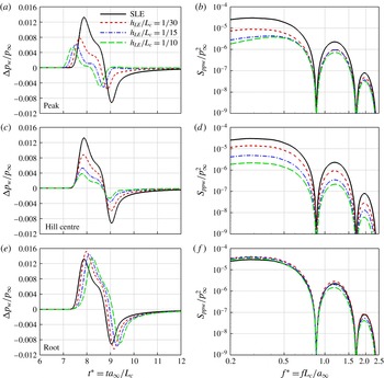
, obtained at three different locations on the WLE (peak, hill centre and the root) for three different values of the WLE amplitude (
 $h_{LE}/L_{c}=1/30$
,
 $1/15$
and
 $1/10$
) with its wavelength fixed (
 $\unicode[STIX]{x1D706}_{LE}/L_{c}=2/15$
), compared with the SLE baseline case.

3.1 Wall and acoustic pressure fluctuations
As a result of the current simulations, figure 4 shows the time signals and corresponding PSD (power spectral density) functions of the wall pressure fluctuation (
 $\unicode[STIX]{x0394}p_{w}$
) on the leading-edge points for three different WLE geometries (
 $h_{LE}/L_{c}=1/30$
,
 $1/15$
and
 $1/10$
) compared with the SLE baseline case. First, it is apparent in the figure that the level of wall pressure fluctuation (aeroacoustic source strength) at the hill location constantly decreases with increasing
 $h_{LE}$
(WLE amplitude) across the entire frequency range. This is directly related to the ‘source cutoff’ effect due to the geometric obliqueness as suggested by Kim et al. (Reference Kim, Haeri and Joseph2016), i.e.
 $\unicode[STIX]{x0394}p_{w}\propto \cos \unicode[STIX]{x1D703}$
where
 $\unicode[STIX]{x1D703}$
is the local sweep angle of the leading edge. Figure 4 also shows that the source strength at the root does not seem to change much with
 $h_{LE}$
(maintained at the level of the SLE case), which might be rather simply anticipated because the sweep angle is locally zero at the root. However, at the peak where the sweep angle is also zero, the source strength significantly changes with
 $h_{LE}$
although it does not drop as consistently as the hill case and seems to converge towards a constant level. The distinction in source strength between the peak and root was also reported by Kim et al. (Reference Kim, Haeri and Joseph2016) with little understood about its cause. Therefore, the main focus of the paper is on understanding and explaining the disparity in source behaviours between the peak and root.
Far-field acoustic pressure time signals,
 $p_{a}^{\prime }(t^{\ast })/p_{\infty }$
, the corresponding PSD,
 $S_{ppa}(f^{\ast })/p_{\infty }^{2}$
and the relative noise reduction spectra,
 $\unicode[STIX]{x0394}\text{SPL}(f^{\ast })$
, obtained at an observer location,
 $\boldsymbol{x}_{o}=(0,5L_{c},0)$
, from three different WLE geometries (
 $h_{LE}/L_{c}=1/30$
,
 $1/15$
and
 $1/10$
with
 $\unicode[STIX]{x1D706}_{LE}/L_{c}=2/15$
), compared with the SLE baseline case.

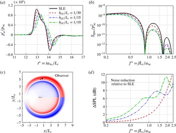
Figure 5 shows the far-field radiated acoustic pressure signals, their PSDs and the relative noise reduction spectra for the three different WLE amplitudes as tested in figure 4. The reduction of the sound pressure level in the WLE cases is clear in this figure. It is also apparent that the noise reduction increases with the WLE amplitude (
 $h_{LE}$
) and with the frequency as well. The same observations have been made in the previous studies with various upstream flow conditions as mentioned in § 1 (Clair et al.
Reference Clair, Polacsek, Garrec, Reboul, Gruber and Joseph2013; Lau et al.
Reference Lau, Haeri and Kim2013; Chaitanya et al.
Reference Chaitanya, Narayanan, Joseph, Vanderwel, Turner, Kim and Gantapathisubramani2015; Narayanan et al.
Reference Narayanan, Chaitanya, Haeri, Joseph, Kim and Polacsek2015; Kim et al.
Reference Kim, Haeri and Joseph2016). The current vortex flow condition adds another example in which the WLE performs successfully for noise reduction. However, it is still unknown as to how the radiated sound field achieves such a large reduction in the high-frequency range (figure 5
b) when the source strength at the peak and root does not drop as much in the same frequency range (figure 4
b,f). On the contrary, the substantially weakened source strength in the low-frequency range at the peak and hill (figure 4
b,d) does not seem to project on the radiated sound field at all (figure 5
b). It is speculated that there exist some crucial mechanisms particularly in the propagation process leading to these controversial results. The authors stress that substantial work is required in order to understand the hidden propagation mechanisms. This paper is yet focused on the source mechanisms which need to be established beforehand.
3.2 Horseshoe vortex systems induced by WLE
As mentioned above, the distinction between the peak and root source behaviours seems contradictory to some extent, as one would assume that both interact with the impinging vortex in a parallel fashion (zero geometric obliqueness). The authors find that the distinction is mainly attributed to the dynamics of secondary vortices created along the WLE. The impinging vortex (rotating clockwise viewed from the
 $xy$
-plane) induces a downwash downstream of its core and consequently an upwash upstream of it as indicated in figure 3. As the vortex moves close to the aerofoil with a SLE the preceding downwash (
 $v<0$
) is suppressed very rapidly to zero (
 $v=0$
) at the leading edge due to the no-penetration (wall) condition. The upshot of this is that a high velocity gradient (
 $\unicode[STIX]{x2202}v/\unicode[STIX]{x2202}x\gg 0$
while
 $\unicode[STIX]{x2202}u/\unicode[STIX]{x2202}y\approx 0$
) is created at the leading edge, which results in a counter-clockwise spanwise vorticity there (
 $\unicode[STIX]{x1D714}_{z}=\unicode[STIX]{x2202}v/\unicode[STIX]{x2202}x-\unicode[STIX]{x2202}u/\unicode[STIX]{x2202}y\gg 0$
). This is a typical example of vortex–body interaction (Rockwell Reference Rockwell1998). In the SLE case the induced spanwise vorticity (
 $\unicode[STIX]{x1D714}_{z}$
) is uniform along the span. However, in a WLE case,
 $\unicode[STIX]{x1D714}_{z}$
varies along the span and also a streamwise vorticity (
 $\unicode[STIX]{x1D714}_{x}$
) is produced due to a significant
 $\unicode[STIX]{x2202}v/\unicode[STIX]{x2202}z$
created at the hill side via the same mechanism described above.
Snapshots of WLE–vortex interaction in temporal order: contour plots for perturbed acoustic pressure (
 $p_{a}^{\prime }/p_{\infty }$
), spanwise vorticity (
 $\unicode[STIX]{x1D714}_{z}L_{c}/a_{\infty }$
) and the
 $Q$
-criterion (
 $\Vert \unicode[STIX]{x1D6FA}_{ij}L_{c}/a_{\infty }\Vert ^{2}-\Vert \unicode[STIX]{x1D61A}_{ij}L_{c}/a_{\infty }\Vert ^{2}$
where
 $\unicode[STIX]{x1D6FA}_{ij}$
and
 $\unicode[STIX]{x1D61A}_{ij}$
are the vorticity and rate of strain tensors, respectively). The figures show secondary vortices (
 $Q$
-criterion) and sound waves (
 $p_{a}^{\prime }/p_{\infty }$
) generated at the leading edge during the interaction. The bottom left corner of images (b–f) provides a zoomed out perspective visualising the radiating sound waves.
 $h_{LE}/L_{c}=1/30$
.

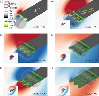
Figure 6 shows snapshots of the WLE–vortex interaction taken as time elapses from the first contact until the vortex completely detaches from the WLE. The vortex travelling through the aerofoil is shown by the spanwise vorticity contour surfaces (
 $\unicode[STIX]{x1D714}_{z}L_{c}/a_{\infty }$
) and the induced secondary vortices on the wall are visualised by using the
 $Q$
-criterion contour surfaces. In addition, the plots of
 $p_{a}^{\prime }/p_{\infty }$
in the
 $xy$
-plane show the dipole sound pulses with an alternating sign being generated when the downwash and upwash strokes of the travelling vortex impact the leading edge.
One of the most critical features shown in figure 6 is the creation of horseshoe-like vortex systems emanating from the WLE as shown from the
 $Q$
-criterion plots. The horseshoe vortex system consists of a bound vortex sitting at the WLE around the peak and two counter-rotating streamwise vortices trailing from the bound vortex as depicted in figure 6(b). The horseshoe vortex systems are created twice during the downwash and upwash strokes, and the direction of the rotation reverses between them. The gap between the pair of streamwise vortices becomes larger as the initial vortex moves further downstream. However, this results in a decreasing gap between two neighbouring streamwise vortices from two adjacent horseshoe vortex systems. This is significantly different vortex dynamics, which does not appear in the SLE case.
 $Q$
-criterion isosurfaces coloured by streamwise vorticity (
 $\unicode[STIX]{x1D714}_{x}L_{c}/a_{\infty }$
) taken at two different points in time during (a) the downwash and (b) upwash strokes of the impinging vortex. The red and blue surfaces indicate positive (clockwise) and negative (anti-clockwise) rotations around the
 $x$
-axis, respectively. The dashed yellow curves indicate the WLE-induced horseshoe vortex systems.

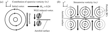
Simplified illustration of the WLE-induced vorticity distribution exhibited in figures 6 and 7: (a) the side view on the WLE showing the contribution of spanwise vorticity components induced during the downwash stroke of the impinging vortex; and, (b) the front view on the WLE describing the streamwise vorticity contribution creating an upwash at the peak and a downwash at the root as a result.

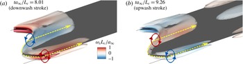
In figure 7 the
 $Q$
-criterion contour surfaces shown in figure 6(b,e) are recoloured by the streamwise vorticity (
 $\unicode[STIX]{x1D714}_{x}L_{c}/a_{\infty }$
) indicating the direction of rotation about the
 $x$
-axis. A brief sketch of this event is provided in figure 8 depicting the horseshoe-vortex-induced vorticity distributions at a single instant of time during the downwash stroke of the impinging vortex. It is illustrated in the figure that, during the downwash stroke, the horseshoe-vortex-induced streamwise vorticity components create an additional downwash at the root but a counteracting upwash at the peak (figure 8
b). For the upwash stroke the opposite trend takes place. On a minor note, the streamwise vorticity distribution observed from the simulation data is almost symmetrical across both sides of the aerofoil with a minor difference in magnitudes.
It is reasonable to assume that the aeroacoustic source strength is almost purely governed by the vertical velocity component (downwash and upwash) impinging on the leading edge since the current aerofoil geometry is completely horizontal with zero thickness and viscosity. Based on this assumption, the authors suggest that the uneven spanwise distribution of the induced vertical velocity illustrated in figure 8(b) is mainly responsible for the disparity in source behaviours between the peak and root observed in § 3.1. It is apparent in the figure 8(b) that the peak is experiencing a reduced level of vertical velocity perturbation due to the counteracting effect of the streamwise vortices, hence a weaker source strength at the peak as seen in figure 4(a,b). On the other hand, the root experiences an amplified level of the vertical velocity perturbation and therefore a reinforced source strength at the root, which is also manifested to a certain extent in figure 4(e,f) (at low frequencies). However, the relative difference to the baseline SLE case is much smaller at the root compared to that taking place at the peak. This requires an explanation. Additional quantitative investigations provided in the following sections reveal further details of the source behaviours.
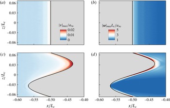
The distribution of maximum values (taken from time signals) of the perturbed vertical velocity (
 $|v|_{max}/a_{\infty }$
) and the vorticity magnitude (
 $|\unicode[STIX]{x1D74E}|_{max}L_{c}/a_{\infty }$
) on the horizontal plane (
 $y=0$
): (a,b) for a SLE baseline case and (c,d) for a WLE case with
 $h_{LE}/L_{c}=1/15$
. The vertical velocity plots are shown in the flow field only and the vorticity magnitude plots on the aerofoil’s upper surface only.

4 Consistent source strength at the root
Figure 9 shows the distribution of the maximum values of the net induced vertical velocity (
 $|v|_{max}/a_{\infty }$
) and vorticity magnitude (
 $|\unicode[STIX]{x1D74E}|_{max}L_{c}/a_{\infty }$
) on the horizontal plane (
 $y=0$
) where the aerofoil is located, obtained from each time signal at every point in space:
 $$\begin{eqnarray}\displaystyle |v|_{max}(\boldsymbol{x})=\max _{t=0}^{\infty }|v(\boldsymbol{x},t)|,\quad |\unicode[STIX]{x1D74E}|_{max}(\boldsymbol{x})=\max _{t=0}^{\infty }|\unicode[STIX]{x1D74E}(\boldsymbol{x},t)|. & & \displaystyle\end{eqnarray}$$
It can be seen in figure 9(c) that the amplitude of the induced vertical velocity is highest around the WLE root area as expected. It is also indicated in figure 9(d) that the streamwise vortices once created at the peak become amplified as they are moving downstream along the hill towards the root, which results in the highly concentrated vertical velocity spot around the root as anticipated from figure 8(b). These are, surprisingly, much higher (by a factor of two) than those of the SLE baseline cases, which leads to a question how such a highly amplified level of velocity perturbation at the root settles down with a minor increase in the aeroacoustic source strength (wall pressure fluctuation) as seen in figure 4(e,f). A discussion on this follows below.
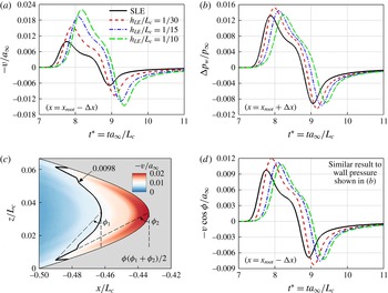
A comparison between the induced vertical velocity and wall pressure fluctuation (
 $v/a_{\infty }$
and
 $\unicode[STIX]{x0394}p_{w}/p_{\infty }$
) at the WLE root for various WLE amplitudes (
 $h_{LE}/L_{c}$
): (a) time signals of
 $v/a_{\infty }$
obtained one grid point upstream of the root; (b) time signals of
 $\unicode[STIX]{x0394}p_{w}/p_{\infty }$
obtained one grid point downstream of the root; (c) an instantaneous contour plot of
 $v/a_{\infty }$
taken at
 $t^{\ast }=8.08$
(when the induced vertical velocity reaches its maximum, for
 $h_{LE}/L_{c}=1/15$
) indicating an oblique interaction with the root, where the values greater than 0.0098 indicate stronger perturbation than the SLE case; and, (d) time signals of
 $v\cos [(\unicode[STIX]{x1D719}_{1}+\unicode[STIX]{x1D719}_{2})/2]/a_{\infty }$
which includes the obliqueness effect. The values of
 $\unicode[STIX]{x1D719}_{1}$
and
 $\unicode[STIX]{x1D719}_{2}$
are listed in table 1.

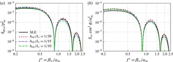
Spectral similarity at the root between the wall pressure fluctuation and the induced vertical velocity including the obliqueness effect: (a) PSD of
 $\unicode[STIX]{x0394}p_{w}/p_{\infty }$
and (b) PSD of
 $v\cos \unicode[STIX]{x1D719}/a_{\infty }$
from figure 10(b,d), respectively.

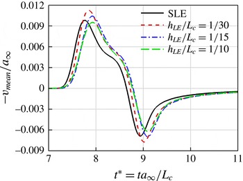
The time signals of the induced vertical velocity impinging at the root are provided in figure 10(a) for various values of
 $h_{LE}$
, where it is clear that the velocity perturbation increases significantly and steadily with
 $h_{LE}$
(linked with the streamwise vorticity intensifying as the WLE becomes slender). On the contrary, the wall pressure fluctuation at the root shown in figure 10(b) does not vary as much, and even slightly decreases with increasing
 $h_{LE}$
. One of the possible answers to this paradoxical event might be related to the fact that the vertical velocity perturbation approaches the root area in an oblique fashion as can be seen from figure 10(c). The vertical velocity isocontours that are skewed and bent around the root area exhibit the oblique interaction taking place. In order to quantify the obliqueness of the interaction, as shown in figure 10(c), two cosine angles (
 $\unicode[STIX]{x1D719}_{1}$
and
 $\unicode[STIX]{x1D719}_{2}$
) are measured from the slender crescent-shaped high-intensity area in which the vertical velocity perturbation is stronger than the maximum value of the SLE case (
 $-v/a_{\infty }=0.0098$
). The angles
 $\unicode[STIX]{x1D719}_{1}$
and
 $\unicode[STIX]{x1D719}_{2}$
are defined between the tip and the two inflection points of the crescent contour line. The authors then take the average of the two measures to represent the overall obliqueness, i.e.
 $\unicode[STIX]{x1D719}=(\unicode[STIX]{x1D719}_{1}+\unicode[STIX]{x1D719}_{2})/2$
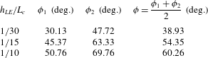
. The values of these angles estimated for each of the cases (
 $h_{LE}/L_{c}=1/30$
,
 $1/15$
and
 $1/10$
) are listed in table 1. The authors have examined the sensitivity of
 $\unicode[STIX]{x1D719}$
for various values of the threshold (up to
 $\pm$
20 % from 0.0098) and found no significant changes as shown in appendix B. Figure 10(d) reveals that the vertical velocity signals multiplied by the obliqueness factor (
 $\cos \unicode[STIX]{x1D719}$
) are remarkably similar to the wall pressure fluctuation signals (
 $\unicode[STIX]{x0394}p_{w}/p_{\infty }$
) given in figure 10(b). They even show the same trend of changes with respect to increasing
 $h_{LE}$
. The remarkable similarity is also demonstrated in the spectral domain in figure 11 where the agreement is consistent throughout the entire frequency range. The result here might strongly suggest that the oblique interaction is one of the possible explanations of the consistent source strength at the root.
The cosine angles representing the oblique interaction between the induced vertical velocity and the WLE shown in figure 10(c).

An additional investigation is performed in this section to find out that there is a certain normalisation applicable to the vertical velocity perturbation, which leads to a meaningful correlation with the wall pressure fluctuation at the root. In this regard, an area-averaged norm of the vertical velocity perturbations is defined around the root as a function of time as follows:
 $$\begin{eqnarray}\displaystyle \left.\begin{array}{@{}c@{}}\displaystyle v_{mean}(t)=\frac{1}{{\mathcal{A}}}\int _{0}^{(1/2)\unicode[STIX]{x1D706}_{LE}}\int _{-(1/2)L_{c}}^{x_{LE}}v(x,y=0,z,t)\,\text{d}x\,\text{d}z,\\ \displaystyle {\mathcal{A}}=\int _{0}^{(1/2)\unicode[STIX]{x1D706}_{LE}}\int _{-(1/2)L_{c}}^{x_{LE}}\,\text{d}x\,\text{d}z=\frac{\unicode[STIX]{x1D706}_{LE}h_{LE}}{\unicode[STIX]{x03C0}},\end{array}\right\} & & \displaystyle\end{eqnarray}$$
where
 ${\mathcal{A}}$
is the area of integration enclosed by the concave part of the WLE sinusoid towards the root and a straight line where the SLE was positioned (e.g. the concave area shown in figure 10
c). The expression for
 $x_{LE}$
as a function of
 $z$
is given in (2.2). The calculated mean vertical velocity signals are presented in figure 12. It is shown that the mean vertical velocity perturbation remains relatively unchanged despite the substantial variation in
 $h_{LE}$
. This might indicate that the overall vertical momentum (created by the initial vortex) is conserved although the vertical velocity tends to surge locally around the root area. The
 $v_{mean}/a_{\infty }$
signals also exhibit a good similarity with the
 $\unicode[STIX]{x0394}p_{w}/p_{\infty }$
(wall pressure fluctuation) signals at the root shown in figure 10(b). Therefore, it may be concluded here that the source strength at the root is better correlated with the mean vertical velocity signal than with the local one nearest to it. This outcome is analogous to the theoretical consideration based on a Poisson equation, i.e.
 $\unicode[STIX]{x1D6FB}^{2}p=-\unicode[STIX]{x1D70C}(\unicode[STIX]{x2202}u_{i}/\unicode[STIX]{x2202}x_{j})(\unicode[STIX]{x2202}u_{j}/\unicode[STIX]{x2202}x_{i})$
– see Tsuji et al. (Reference Tsuji, Fransson, Alfredsson and Johansson2007) – indicating that pressure at a certain location is determined by integrating velocity properties surrounding it.
Mean vertical velocity signals calculated from (4.2) around the root area for various values of
 $h_{LE}/L_{c}$
(WLE amplitude), in relation to the consistent source strength at the root irrespective of
 $h_{LE}$
.

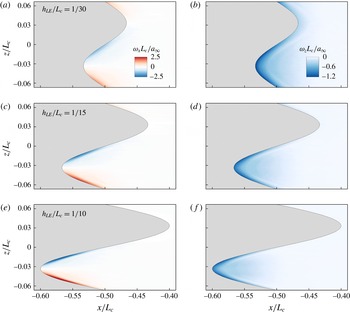
Instantaneous contour plots of streamwise vorticity (
 $\unicode[STIX]{x1D714}_{x}L_{c}/a_{\infty }$
: left) and spanwise vorticity (
 $\unicode[STIX]{x1D714}_{z}L_{c}/a_{\infty }$
: right) on the upper surface of the aerofoil for three different WLE amplitudes, obtained when the induced vertical velocity in front of the peak reaches its maximum amplitude: (a,b)
 $ta_{\infty }/L_{c}=7.540$
, (c,d) 7.461 and (e,f) 7.305 – see figure 15(a).

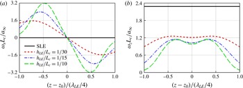
Vorticity distributions in span along the leading edge for various values of
 $h_{LE}/L_{c}$
obtained when the induced vertical velocity in front of the peak reaches its maximum amplitude: (a) streamwise vorticity (
 $\unicode[STIX]{x1D714}_{x}L_{c}/a_{\infty }$
) and (b) spanwise vorticity (
 $\unicode[STIX]{x1D714}_{z}L_{c}/a_{\infty }$
) on the upper surface of the aerofoil – see figure 13. The spanwise coordinate of the peak is denoted by
 $z_{0}$
in the
 $x$
-axis labels.

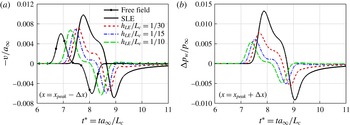
A comparison between the induced vertical velocity and wall pressure fluctuation (
 $v/a_{\infty }$
and
 $\unicode[STIX]{x0394}p_{w}/p_{\infty }$
) at the WLE peak for various WLE amplitudes (
 $h_{LE}/L_{c}$
): (a) time signals of
 $v/a_{\infty }$
obtained one grid point upstream of the peak; and, (b) time signals of
 $\unicode[STIX]{x0394}p_{w}/p_{\infty }$
obtained one grid point downstream of the peak. The case with ‘Free field’ indicates a free-field solution (without the aerofoil) recorded at
 $(x,y)=(-0.7L_{c},0)$
.

5 Variations in source strength at the peak
The focus is now moved on to the WLE peak in this section. It has been observed earlier in § 3 that the aeroacoustic source characteristics at the peak are considerably different to those at the root. The source strength at the peak decreases significantly with increasing WLE amplitude (
 $h_{LE}$
) as shown in figure 4(a,b). It seemed rather straightforward from figure 8(b) that this was due to the attenuating vertical velocity contribution created at the peak by the streamwise vorticity components that are growing with
 $h_{LE}$
as shown in figures 13 and 14. The significant growth of the streamwise vorticity appears counterbalanced by a decay in the spanwise vorticity to a certain extent, which corresponds to Helmholtz’s theorems. The time signals of the induced vertical velocity and the corresponding wall pressure fluctuation at the peak varying with
 $h_{LE}$
are shown in figure 15. It is apparent in the figure that the vertical velocity perturbation decreases with increasing
 $h_{LE}$
and it results in the reduction of the source strength at the peak. A more interesting observation, however, is that both
 $v$
and
 $\unicode[STIX]{x0394}p_{w}$
become significantly less sensitive to increasing
 $h_{LE}$
after a certain point. In particular the
 $v$
signal seems to converge towards that of the free-field solution generated without the aerofoil in place. This section is focused on explaining the mechanism of the inconsistent source behaviours taking place at the peak.
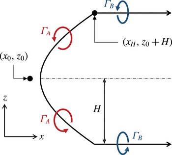
Schematic of the horseshoe vortex (HV) system used to estimate the WLE-induced vertical velocity in front of the peak, in relation to (5.3).

Considering the horseshoe vortex (HV) system identified in § 3, a semi-analytic approach based on Biot–Savart’s law is proposed in order to obtain more information on the induced velocity components from the HV system. The general form of Biot–Savart’s law is expressed by
 $$\begin{eqnarray}\displaystyle \text{d}\boldsymbol{v}(\boldsymbol{x}_{0},\boldsymbol{l})=\frac{\unicode[STIX]{x1D6E4}}{4\unicode[STIX]{x03C0}}\frac{\boldsymbol{r}\times \text{d}\boldsymbol{l}}{|\boldsymbol{r}|^{3}},\quad \boldsymbol{r}=\boldsymbol{l}-\boldsymbol{x}_{0}, & & \displaystyle\end{eqnarray}$$
where
 $\boldsymbol{x}_{0}$
and
 $\boldsymbol{l}$
are position vectors of the observer and a certain point on the vortex filament, respectively; and,
 $\unicode[STIX]{x1D6E4}$
is the cross-sectional circulation induced by the vortex. Since the current HV system is on a horizontal plane, the above equation with the observer position fixed at the peak can be simplified as
 $$\begin{eqnarray}\displaystyle \text{d}v_{peak}^{HV}=\frac{\unicode[STIX]{x1D6E4}}{4\unicode[STIX]{x03C0}}\frac{(r_{3}\,\text{d}x-r_{1}\,\text{d}z)}{(r_{1}^{2}+r_{3}^{2})^{3/2}}, & & \displaystyle\end{eqnarray}$$
where the subscripts ‘1’ and ‘3’ denote the streamwise and spanwise coordinates, respectively. Integrating all contributions from the bound vortex and the two trailing vortices lead to the following formula (see figure 16):
 $$\begin{eqnarray}\displaystyle \left.\begin{array}{@{}c@{}}\displaystyle v_{peak}^{HV}=v_{A}+v_{B},\\ \displaystyle v_{A}=\frac{1}{4\unicode[STIX]{x03C0}}\int _{z_{0}-H}^{z_{0}+H}\frac{\unicode[STIX]{x1D6E4}_{A}}{[(x_{LE}-x_{0})^{2}+(z-z_{0})^{2}]^{3/2}}\left[(z-z_{0})\frac{\text{d}x_{LE}}{\text{d}z}-(x_{LE}-x_{0})\right]\text{d}z,\\ \displaystyle v_{B}=\frac{H}{2\unicode[STIX]{x03C0}}\int _{x_{H}}^{\infty }\frac{\unicode[STIX]{x1D6E4}_{B}\,\text{d}x}{[(x-x_{0})^{2}+H^{2}]^{3/2}},\end{array}\right\} & & \displaystyle\end{eqnarray}$$
where the subscripts ‘
 $A$
’ and ‘
 $B$
’ represent contributions from the bound and trailing vortices, respectively;
 $(x_{0},z_{0})=(-L_{c}/2-h_{LE}-\unicode[STIX]{x0394}x,-\unicode[STIX]{x1D706}_{LE}/4)$
is the observer position (one grid cell ahead of the peak point) – see (2.2); and,
 $H$
is the half-width of the HV. The bound vortex is located along the WLE,
 $x=x_{LE}(z)$
that is given by (2.2), and
 $x_{H}=x_{LE}(z_{0}+H)$
is the starting
 $x$
-coordinate of the trailing vortices. Here,
 $x_{H}$
is selected at the position where the largest streamwise vorticity
 $|\unicode[STIX]{x1D714}_{x}|$
is obtained.
In (5.3), the cross-sectional circulations
 $\unicode[STIX]{x1D6E4}_{A}$
and
 $\unicode[STIX]{x1D6E4}_{B}$
are calculated at each grid point along the HV based on the simulation data by using the Stokes’ theorem with a constraint for the
 $Q$
-criterion as
 $$\begin{eqnarray}\displaystyle \unicode[STIX]{x1D6E4}=\left.\int _{{\mathcal{A}}}\unicode[STIX]{x1D714}_{n}\,\text{d}{\mathcal{A}}\right|_{Q>max(Q)/100}, & & \displaystyle\end{eqnarray}$$
where
 ${\mathcal{A}}$
is the integration area on a plane that is perpendicular to the WLE curve and accordingly
 $\unicode[STIX]{x1D714}_{n}$
is the vorticity component normal to the plane. The
 $Q$
-criterion constraint is used to eliminate the circulation produced by the initial prescribed vortex in the current evaluation. Since the prescribed vortex has a significantly lower strength, a value blanking method can be adopted for this purpose. This is achieved by restricting
 ${\mathcal{A}}$
to the region where the
 $Q$
-criterion remains above 1 % of the global maximum value. Since the HV structure exists on both the upper and lower sides of the aerofoil, the calculation is repeated for both and added together to obtain the total induced velocity.
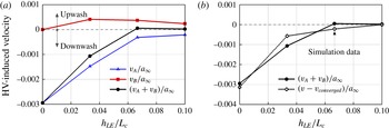
Semi-analytic predictions of the HV-induced vertical velocity components in front of the peak, obtained by using (5.3) for various values of
 $h_{LE}/L_{c}$
: (a) contributions from the bound vortex (
 $v_{A}$
) and the trailing vortices (
 $v_{B}$
), and the total (
 $v_{A}+v_{B}$
); (b) a comparison between the semi-analytic result and direct simulation data (‘
 $v_{converged}$
’ is represented by the case with
 $h_{LE}/L_{c}=1/10$
). The predictions are made at
 $ta_{\infty }/L_{c}=7.774$
, 7.540, 7.461 and 7.305 for
 $h_{LE}/L_{c}=0$
,
 $1/30$
,
 $1/15$
and
 $1/10$
, respectively, when the vertical velocity reaches its maximum amplitude (see figure 15).


The result of the semi-analytic prediction by using (5.3) for the HV-induced vertical velocity in front of the peak is presented in figure 17. The semi-analytic result follows a very similar trend to that from the simulation data albeit not fully matched. It is clearly shown in figure 17(a) that the net HV-induced vertical velocity decays with increasing
 $h_{LE}$
. This is due to the contributions from the bound and trailing vortices (
 $v_{A}$
and
 $v_{B}$
) cancelling out each other. The mutual cancellation is almost perfect and resulting in a zero sum when
 $h_{LE}/L_{c}=1/15$
or higher, in which case the overall vertical velocity is effectively maintained by the initial vortex approaching (free-field solution). This explains the convergence/saturation of the vertical velocity signal at the peak for high
 $h_{LE}/L_{c}$
, which was questioned in the beginning of the section.
In the meantime, in figure 17, the contribution of the bound vortex (
 $v_{A}$
) decreases rapidly and converges towards zero with increasing
 $h_{LE}$
. The rapid decay of
 $v_{A}$
is considered to be the major cause of the reduction in source strength at the peak discussed earlier (figure 15). This may be explained in three steps. First, between
 $h_{LE}=0$
(SLE) and
 $1/30$
, there is a large drop in the spanwise vorticity (
 $\unicode[STIX]{x1D714}_{z}$
) and the appearance of
 $\unicode[STIX]{x1D714}_{x}$
, which are shown in figure 14. Secondly, between
 $h_{LE}=1/30$
and
 $1/15$
, there is a moderate drop in
 $\unicode[STIX]{x1D714}_{z}$
and a further growth in
 $\unicode[STIX]{x1D714}_{x}$
leading to a continued reduction of
 $v_{A}$
up to this point. Lastly, between
 $h_{LE}=1/15$
and
 $1/10$
,
 $\unicode[STIX]{x1D714}_{x}$
still grows consistently (with very little change in
 $\unicode[STIX]{x1D714}_{z}$
); however, this does not reflect efficiently on
 $v_{A}$
due to the fact that the term
 $[(z-z_{0})\,\text{d}x_{LE}/\text{d}z-(x_{LE}-x_{0})]$
in (5.3) tends to zero or a very small number (except for the area nearest to the peak where
 $\unicode[STIX]{x1D714}_{z}$
prevails) since
 $\text{d}x_{LE}/\text{d}z\sim (x_{LE}-x_{0})/(z-z_{0})$
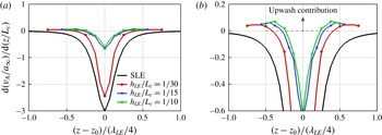
as the WLE profile becomes increasingly slender (similar to a long and narrow triangle). These trends can also be found in figure 18 which provides local piecewise contributions of the bound vortex (
 $\text{d}v_{A}/\text{d}z$
as a function of
 $z$
) showing the rapid decrease of the bound vortex contribution and its convergence at high
 $h_{LE}/L_{c}$
. The figure also shows a certain amount of upwash generated by the bound vortex indicating the influence of the streamwise vorticity component prevalent around the edges of the bound vortex.
More information can be found from the semi-analytic prediction data. In figure 17 the contribution of the trailing vortices (
 $v_{B}$
) seems to gradually decreases with increasing
 $h_{LE}$
although the streamwise vorticity (
 $\unicode[STIX]{x1D714}_{x}$
) grows steadily with
 $h_{LE}$
as shown in figures 13 and 14. It may be explained by using (5.3) where
 $v_{B}$
is proportional to
 $H$
and asymptotically to
 $(x_{H}-x_{0})^{-3}$
. For a higher
 $h_{LE}$
,
 $H$
decreases and
 $x_{H}$
increases (as shown in figures 14 and 16), which may result in a reduced
 $v_{B}$
despite a higher
 $\unicode[STIX]{x1D714}_{x}$
or
 $\unicode[STIX]{x1D6E4}_{B}$
.
6 Additional findings and discussion
This section briefly presents additional findings made with regard to two different aspects based on the current simulation framework: (i) the relationship between the aeroacoustic source strength and the WLE aspect ratio; and, (ii) the effect of a three-dimensional profile introduced in the impinging vortex on the interaction with the leading-edge geometries.
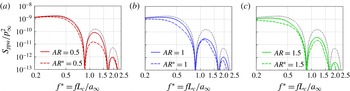
Far-field acoustic pressure PSD profiles,
 $S_{ppa}(f^{\ast })/p_{\infty }^{2}$
, obtained at an observer location,
 $\boldsymbol{x}_{o}=(0,5L_{c},0)$
, for three different WLE aspect ratios (
 $AR=2h_{LE}/\unicode[STIX]{x1D706}_{LE}=0.5$
, 1 and 1.5). The aspect ratios with ‘*’ indicate that the size of the WLE is doubled (
 $AR^{\ast }=2h_{LE}^{\ast }/\unicode[STIX]{x1D706}_{LE}^{\ast }$
where
 $h_{LE}^{\ast }=2h_{LE}$
and
 $\unicode[STIX]{x1D706}_{LE}^{\ast }=2\unicode[STIX]{x1D706}_{LE}$
). The dotted curves are from the SLE baseline case.

6.1 WLE aspect ratio and source strength
A parametric study is carried out to find a relationship between the aeroacoustic source strength and the WLE aspect ratio (
 $AR=2h_{LE}/\unicode[STIX]{x1D706}_{LE}$
). Three different values of
 $AR=0.5$
, 1 and 1.5 have been studied in §§ 3–5 with the wavelength fixed at
 $\unicode[STIX]{x1D706}_{LE}/L_{c}=2/15$
. In this section, additional simulations are performed with both
 $h_{LE}$
and
 $\unicode[STIX]{x1D706}_{LE}$
doubled (hence, the aspect ratios remain the same) in order to investigate the differences in the source characteristics. In terms of the radiated sound pressure level (SPL), it is well known that the SPL is dependent largely on
 $h_{LE}$
with secondary contributions from
 $\unicode[STIX]{x1D706}_{LE}$
(Lau et al.
Reference Lau, Haeri and Kim2013; Chaitanya et al.
Reference Chaitanya, Narayanan, Joseph, Vanderwel, Turner, Kim and Gantapathisubramani2015; Narayanan et al.
Reference Narayanan, Chaitanya, Haeri, Joseph, Kim and Polacsek2015; Kim et al.
Reference Kim, Haeri and Joseph2016). This means that the SPL would be further reduced in the cases of doubled
 $h_{LE}$
for the same aspect ratio, which is also true in the current study as shown in figure 19 (
 $AR^{\ast }=0.5$
, 1 and 1.5). The further reduction of sound is apparent across the whole frequency range. However, the reduced sound does not necessarily relate to a reduced source strength as far as the current results are concerned – see below.
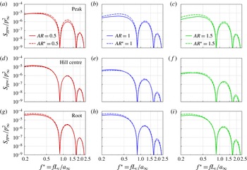
Wall pressure PSD profiles,
 $S_{ppw}(f^{\ast })/p_{\infty }^{2}$
, obtained at three different locations on the WLE (peak, hill centre and the root) for three different WLE aspect ratios (
 $AR=2h_{LE}/\unicode[STIX]{x1D706}_{LE}=0.5$
, 1 and 1.5). The aspect ratios with ‘*’ indicate that the size of the WLE is doubled (
 $AR^{\ast }=2h_{LE}^{\ast }/\unicode[STIX]{x1D706}_{LE}^{\ast }$
where
 $h_{LE}^{\ast }=2h_{LE}$
and
 $\unicode[STIX]{x1D706}_{LE}^{\ast }=2\unicode[STIX]{x1D706}_{LE}$
).

Figure 20 shows the source strength (wall pressure spectra) at the peak, hill centre and root, obtained from the additional simulations with double sized WLEs, compared with the earlier original cases of the same aspect ratios. It is noticeable that the source strength remains relatively unchanged by doubling the size of the WLE as far as the aspect ratio is maintained. Although slightly large deviations are seen at the peak at some frequencies, a remarkable level of similarities can be found at the root and the hill. The result might suggest that the WLE aspect ratio is a similarity parameter which dictates the source strength and characteristics, despite the radiated sound being influenced mainly by the WLE amplitude. It also suggests that there exist imperative mechanisms contributing to the noise reduction purely associated with the propagation of the sound waves.
One of the propagation effects was indicated by Kim et al. (Reference Kim, Haeri and Joseph2016) where it was shown that phase interferences between the source signals make significant contributions to the reduction of the radiated sound at certain frequencies with out-of-phase relationships. The phase interference effect may also be related with the starting frequency of noise reduction,
 $f_{0}\approx 0.25U_{\infty }/h_{LE}$
, reported by Narayanan et al. (Reference Narayanan, Chaitanya, Haeri, Joseph, Kim and Polacsek2015). This implies that the low-frequency noise reduction is strongly dependent of the WLE amplitude. However, apart from these, there is little known about the propagation mechanisms particularly with regard to the discrepancies between the source spectra and the radiated sound spectrum as highlighted towards the end of § 3.1. It is envisaged that the similarity in the source characteristics observed in this paper will facilitate the study of the propagation mechanisms in the future if two different WLEs with the same aspect ratio are investigated and compared against each other.
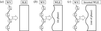
Schematics of a wavy vortex (WV) interacting with three different leading-edge geometries: (a) SLE, (b) WLE and (c) the WLE inverted. The centreline of the wavy vortex is undulated along the span in the same fashion applied to the WLE profile – based on (2.2). The inverted WLE (IWLE) has an out-of-phase formation against the prescribed WV.

6.2 The effect of three-dimensional profile in the impinging vortex
A miscellaneous test has been performed in order to briefly demonstrate the effect of three-dimensionality introduced in the impinging vortex on the interaction with the leading-edge geometries. The schematics of the additional test cases are described in figure 21. The centreline of the impinging vortex no longer remains straight but forms a wavy profile in the same fashion that was applied to the WLEs in the paper. Three additional cases of aerofoil–vortex interaction are considered as depicted in figure 21: (a) WV-SLE, (b) WV-WLE and (c) WV-IWLE, where WV and IWLE stand for wavy vortex and inverted WLE, respectively. The WV and WLE profiles are identical but the IWLE (inverted WLE) has an
 $180^{\circ }$
phase shift against the WV. The WV profile is created simply by changing the centre coordinate (
 $x_{0}$
) of the vortex used in (2.5) and (2.6) as follows:
 $$\begin{eqnarray}\displaystyle x_{0}=-2.5L_{c}+h_{LE}\sin \left(\frac{2\unicode[STIX]{x03C0}z}{\unicode[STIX]{x1D706}_{LE}}\right),\quad z\in \left[-\frac{1}{2}L_{z},\frac{1}{2}L_{z}\right]. & & \displaystyle\end{eqnarray}$$
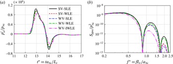
The result of the additional simulations is presented in figure 22 in comparison with the earlier cases (SV-SLE and SV-WLE) that was based on a straight vortex (SV). It is shown that the WV-WLE case yields an almost identical sound pressure spectrum to that of the SV-SLE case. Also, the WV-SLE and SV-WLE cases are remarkably similar to each other except a marginal difference at high frequencies. In comparison, the WV-IWLE case exhibits a substantial noise reduction across a wide range of frequencies. These results could be explained by looking at the streamwise distance between the impinging vortex and the leading edge. First, the WV-WLE and SV-SLE cases have the same relative distance that is constant along the span. Therefore the impact takes place synchronously (with no time delay) across the span. The WV-SLE and SV-WLE cases also have the same relative distance but varying along the span, which results in an asynchronous interaction over the span, hence a reduced noise level. Finally, the WV-IWLE case is effectively comparable to the SV-WLE case with the WLE amplitude doubled (
 $h_{LE}/L_{c}=1/15$
instead of
 $1/30$
) and therefore resulting in a significantly increased noise reduction (see figure 5).
Far-field acoustic pressure time signals and the corresponding PSD: (a)
 $p_{a}^{\prime }(t^{\ast })/p_{\infty }$
and (b)
 $S_{ppa}(f^{\ast })/p_{\infty }^{2}$
obtained at an observer location,
 $\boldsymbol{x}_{o}=(0,5L_{c},0)$
, from the additional simulations described in figure 21. The new results are compared with the earlier cases (SV-SLE and SV-WLE) that used a straight vortex. The WLE and WV profiles are based on
 $h_{LE}/L_{c}=1/30$
and
 $\unicode[STIX]{x1D706}_{LE}/L_{c}=2/15$
.

It is possible to consider more complex cases such as the wavy vortex has a different wavelength, amplitude or phase shift to those of the wavy leading edge to interact with. Also, the impinging vortex can be finite in span (similar to an individual eddy) as explored in Mathews & Peake (Reference Mathews and Peake2015). Studying these increasingly complex cases may enhance the understanding of the noise generation/reduction mechanisms into more details later on.
7 Concluding remarks
Detailed understanding of the aeroacoustic source mechanisms of a thin aerofoil with a WLE interacting with a prescribed impinging vortex has been achieved by using high-order accurate aeroacoustics simulations in this paper. The numerical flow visualisation showed that the WLE upon interaction with the impinging vortex created a HV system stemming from the peak area. The HV-induced vorticity and velocity fields around the WLE provided key information to quantify and understand the changes in the wall pressure fluctuation compared to the SLE baseline cases. Two distinctive source behaviours were observed and questioned during the initial analysis of the simulation data. Some scientific explanations to the questions have emerged after investigating into the role of the HV system and the induced velocity field induced by it.
The aeroacoustic source strength at the root remained consistent (similar to that of the SLE counterpart) irrespective of the WLE amplitude (
 $h_{LE}$
). This initially seemed incompatible with the growing contribution of the HVs substantially amplifying the vertical velocity perturbation around the root with increasing
 $h_{LE}$
. The current investigation showed that the oblique interaction between the vertical velocity perturbation and the root area could be one of the mechanisms to explain the paradoxical event. From another point of view, it was demonstrated that the area-averaged vertical velocity remained at a constant level irrespective of
 $h_{LE}$
(indicating the conservation of vertical momentum), which might suggest that the source strength at the root was determined mainly by the overall amount of vertical momentum possessed in the upstream of the root.
Unlike the root, the source strength at the peak was significantly reduced with increasing
 $h_{LE}$
up to a certain point. The reduction of source strength at the peak was well correlated with the growth in streamwise vorticity and the decay in the spanwise vorticity along the HV which efficiently attenuated the vertical velocity perturbation. However, the source strength at the peak ceased to decrease further when
 $h_{LE}$
was sufficiently large. The source convergence/saturation event was explained by using a semi-analytic model of the HV (a curved bound vortex connected with two straight trailing vortices) based on Biot–Savart’s law. The semi-analytic model showed that the HV-induced downwash and upwash components eventually led to a complete mutual cancellation as
 $h_{LE}$
becomes large, and therefore the net vertical velocity in front of the peak converged to that of the free-field solution with no aerofoil in place. It was also found that the highly slender WLE geometry made the HV effectively non-responsive to the source strength at the peak despite the intensified streamwise vorticity components surrounding it.
It appeared that there was a strong similarity rule existing in the source characteristics between two different WLE geometries with the same aspect ratio. The level of similarity viewed from the wall pressure spectra was maintained at all frequencies and all probing points (peak, hill centre and root). This might suggest that the source mechanisms explained in this paper have a certain level of universality applicable to a wide range of WLE geometries. The authors suggest within this hypothesis that it is necessary to investigate the ‘propagation’ mechanisms in detail since there is a significant disagreement between the source power spectra at the wall and the noise reduction spectrum at the far field, as addressed in § 3.1. Also, the exponential growth of noise reduction with frequency – reported repeatedly by Chaitanya et al. (Reference Chaitanya, Narayanan, Joseph, Vanderwel, Turner, Kim and Gantapathisubramani2015), Narayanan et al. (Reference Narayanan, Chaitanya, Haeri, Joseph, Kim and Polacsek2015), Kim et al. (Reference Kim, Haeri and Joseph2016) – is unexplained solely by the source mechanisms.
The current study was focused on the most basic scenario where the impinging vortex was kept two-dimensional and only the leading-edge geometry was changed from 2-D to 3-D such that it was straightforward to identify the differences that the geometric modification made to the flow and sound. It would be necessary afterwards to consider a more complex case where the impinging vortex has a three-dimensional profile as briefly demonstrated in § 6.2. It will aid better understanding the realistic aerofoil-turbulence interaction that has a certain spanwise length scale and coherence. The size of the parametric space to explore will become substantial in that case though.
Acknowledgements
The authors gratefully acknowledge the support of EPSRC (Engineering and Physical Sciences Research Council) for the present work under the CDT (Centre for Doctoral Training) grant EP/G03690X/1 and the ICSS (Institute for Complex Systems Simulation) at the University of Southampton. We also acknowledge the high-performance computing facilities and services of the UK National Supercomputer ARCHER via the support of UK Turbulence Consortium (EP/L000261/1) and the local IRIDIS4 at the University of Southampton in the completion of this work. All data supporting this study are openly available from the University of Southampton repository at http://dx.doi.org/10.5258/SOTON/403598.
Appendix A. Validation of computational data
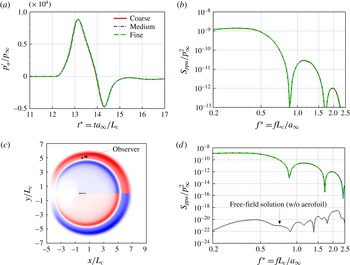
Figure 23 shows the results of a grid convergence test conducted with a WLE geometry:
 $h_{LE}/L_{c}=1/15$
and
 $\unicode[STIX]{x1D706}_{LE}/L_{c}=2/15$
(
 $AR=1$
). Three different levels of grid resolution (coarse, medium and fine) were used. The medium level was used for all simulation data presented in this paper. The coarse/fine levels have 20 % less/more resolution in all directions. The number of grid points and the typical mesh sizes used for each resolution level are listed in table 2. Figure 23(a,b) demonstrates that there is effectively no difference in the results (time signals and the spectra as well) between the three different grids. Figure 23(d) also shows a comparison to the free-field solution obtained without the aerofoil in place (using the medium grid). The level of background noise (numerical error residual) remained at least 40 dB lower than the physical SPL throughout the entire frequency range, which represents the quality of the numerical solutions presented in this paper.
A grid convergence test of the current numerical simulation by using three different levels of grid resolution. The far-field acoustic pressure signal (
 $p_{a}^{\prime }/p_{\infty }$
) and its PSD (
 $S_{ppa}/p_{\infty }^{2}$
) are obtained at an observer point
 $\boldsymbol{x}_{0}=(0,5L_{c},0)$
. The WLE geometry is based on
 $h_{LE}/L_{c}=1/15$
and
 $\unicode[STIX]{x1D706}_{LE}/L_{c}=2/15$
(corresponding to figure 5).

Supplementary information for the grid convergence test shown in figure 23, where
 $n_{\unicode[STIX]{x1D709}}$
,
 $n_{\unicode[STIX]{x1D702}}$
and
 $n_{\unicode[STIX]{x1D701}}$
denote the number of grid cells in the
 $\unicode[STIX]{x1D709}$
-,
 $\unicode[STIX]{x1D702}$
- and
 $\unicode[STIX]{x1D701}$
-directions, respectively – see (2.3) and (2.4).

Appendix B. Sensitivity test for the measure of the obliqueness in interaction
Tables 3–5 show the estimated angles of the oblique interaction (
 $\unicode[STIX]{x1D719}$
) described in § 4 for various values of the
 $-v/a_{\infty }$
contour threshold selected from figure 10(c). The sensitivity test was performed for all three WLE geometries used in the paper (
 $h_{LE}/L_{c}=1/30$
,
 $1/15$
and
 $1/10$
). The tables show that the choice of the threshold (within the 40 % bandwidth tested) makes an insignificant change to the estimated obliqueness angle with a deviation of up to 4.07 % at maximum as far as the current test cases are concerned.
The estimation of
 $\unicode[STIX]{x1D719}$
for various thresholds in the case of
 $h_{LE}/L_{c}=1/30$
.

The estimation of
 $\unicode[STIX]{x1D719}$
for various thresholds in the case of
 $h_{LE}/L_{c}=1/15$
.

The estimation of
 $\unicode[STIX]{x1D719}$
for various thresholds in the case of
 $h_{LE}/L_{c}=1/10$
.